| Issue |
A&A
Volume 695, March 2025
|
|
|---|---|---|
| Article Number | A172 | |
| Number of page(s) | 20 | |
| Section | Celestial mechanics and astrometry | |
| DOI | https://doi.org/10.1051/0004-6361/202453545 | |
| Published online | 19 March 2025 | |
Influence of a continuous plane gravitational wave on Gaia-like astrometry
1
Lohrmann Observatory, Technische Universität Dresden,
Mommsenstraße 13,
01062
Dresden, Germany
2
Lund Observatory, Division of Astrophysics, Department of Physics, Lund University,
Box 43,
22100
Lund, Sweden
3
European Space Agency (ESA), European Space Astronomy Centre (ESAC), Camino bajo del Castillo, s/n, Urbanización Villafranca del Castillo, Villanueva de la Cañada,
28692
Madrid, Spain
★ Corresponding author; This email address is being protected from spambots. You need JavaScript enabled to view it.
Received:
20
December
2024
Accepted:
24
January
2025
Abstract
Context. A gravitational wave (GW) passing through an astrometric observer causes periodic shifts of the apparent star positions measured by the observer. For a GW of sufficient amplitude and duration, at a suitable frequency, these shifts might be detected with a Gaia-like astrometric telescope.
Aims. This paper is aimed at making a detailed analysis of the effects of GWs on an astrometric solution based on Gaia-like observations, which are one-dimensional and strictly differential between two widely separated fields of view, following a prescribed scanning law.
Methods. We present a simple geometric model for the astrometric effects of a plane GW in terms of the time-dependent positional shifts. Using this model, we discuss the general interaction between the GW and a Gaia-like observation. Numerous Gaia-like astrometric solutions have been computed, taking as input simulated observations that include the effects of a continuous plain GW with constant parameters and periods ranging from ~50 days to 100 years. The resulting solutions have been analysed in terms of the systematic errors on astrometric and attitude parameters, as well as the observational residuals.
Results. We found that a significant part of the GW signal is absorbed by the astrometric parameters, leading to astrometric errors of a magnitude (in radians) comparable to the strain parameters. These astrometric errors are generally impossible to detect because the true (unperturbed) astrometric parameters are not known with a corresponding level of accuracy. The astrometric errors are especially large for specific GW frequencies that are linear combinations of two characteristic frequencies of the scanning law. Nevertheless, for all GW periods smaller than the time span covered by the observations, significant parts of the GW signal also go into the astrometric residuals. This fosters the hope for a GW detection algorithm based on the residuals of standard Gaia-like astrometric solutions.
Key words: gravitational waves / methods: numerical / methods: observational / catalogs / astrometry
© The Authors 2025
 Open Access article, published by EDP Sciences, under the terms of the Creative Commons Attribution License (https://creativecommons.org/licenses/by/4.0), which permits unrestricted use, distribution, and reproduction in any medium, provided the original work is properly cited.
This article is published in open access under the Subscribe to Open model. This email address is being protected from spambots. You need JavaScript enabled to view it. to support open access publication.
1 Introduction
The fact that a gravitational wave (GW) causes astrometric effects has been known and analysed for quite some time (Braginsky et al. 1990; Pyne et al. 1996; Kaiser & Jaffe 1997; Gwinn et al. 1997; Kopeikin et al. 1999; Book & Flanagan 2011). Since the high-accuracy astrometry of Gaia has become a reality (e.g. Gaia Collaboration 2023), there has been rising interest in investigating GW effects specifically for these (or similar) astrometric observations (e.g. Klioner 2018; O…Beirne & Cornish 2018; Mihaylov et al. 2018; Moore et al. 2017; Bini & Geralico 2018; Darling et al. 2018; Çalışkan et al. 2024).
Indeed, Gaia astrometry, as it is not only of microarcsecond accuracy, but also global, offers interesting possibilities to investigate GWs. However, it is very important to note that the specific observational principles of astrometric scanning satellites (Lindegren & Bastian 2010; Gaia Collaboration 2016) are properly taken into account. One example is the fact that the instantaneous pointing (attitude) of the satellite must be determined from its own astrometric observations and that the observations of a Gaia-like astrometric instrument are effectively one-dimensional (1D). Another aspect is the prescribed observational schedule known as the scanning law. Although Klioner (2018) has taken these specifics into account, that is often not the case in other publications.
It is known from the literature cited above that a GW passing through an astrometric observer causes apparent, timedependent shifts of the positions of astrometric sources. The direction and magnitude of the shift depends on time, the celestial position of the astrometric source, and the parameters of the GW (e.g. Book & Flanagan 2011; Klioner 2018). The GW effect in astrometry is global in the sense that it can be detected over a large fraction of the sky, if it is at all detectable. This is so because the amplitude of the shift is proportional to sin θ, where θ is the angular distance between the source and the direction of propagation of the GW. Moreover, the effect does not depend on the distance to the astrometric source, as long as it is much greater that the wavelength of the GW (e.g. Book & Flanagan 2011). These properties make global astrometry especially interesting for the study of possible GW signals.
This paper is the first in a series of publications discussing the interaction of GW signals with astrometric observations made from a Gaia-like scanning telescope. In particular, this paper is devoted to a detailed discussion of the effects that a single plane continuous GW has on a Gaia-like astrometric solution.
For several reasons, the effects of GWs cannot be part of the standard relativistic model for high-accuracy astrometry (see e.g. Klioner 2003, 2004 describing the model used for Gaia). The standard relativistic model is intended to correct for all accurately known relativistic effects, such as those coming from the gravitational field of the Solar System. However, no GW sources producing relevant astrometric effects are currently known. On the other hand, without good a priori estimates of the GW parameters, it is not (in practice) feasible to include the GW parameters as unknowns in the global astrometric solution, which is essentially a linear (or weakly non-linear) least-squares estimation. Presently, the only practicable approach is therefore to apply a dedicated detection algorithm to the residuals of a standard astrometric solution. This is the topic of a separate publication in this series.
A detailed introduction to the standard astrometric solution used for Gaia can be found in Lindegren et al. (2012). Given that this solution is a simultaneous determination of the astrometric (source) parameters, the spacecraft attitude, and the calibration parameters, it is not clear a priori to what extent an un-modelled GW signal in the data is absorbed by these solution unknowns and, therefore, it merely produces a biased astrometric solution; in addition, we do not know to what extent it goes into the residuals instead, where it could be detected by a dedicated post-processing algorithm.
The goal of this first paper is precisely to give a detailed qualitative and quantitative description of the effects that an individual GW will have on a Gaia-like global astrometric solution and its residuals. We present both theoretical and numerical results to illustrate the effects. The investigation is limited to the case of a single plane continuous GW with constant parameters, but considering a wide range of the parameters.
The structure of the paper is as follows. Section 2 presents the key parameters of the GW model and a brief overview of the astrometric effects of a GW. In Sect. 3, we discuss the mechanism of interaction between a GW signal and a Gaia-like astrometric solution. Section 4 describes the numerical simulations used in this study. Simulation results are presented in Sect. 5 and summarised in Sect. 6.
Additional details are given in appendices. Appendix A gives a simple geometric description of the apparent positional shifts from a GW, providing new insight into the nature of the astrometric effects. Appendix B gives a statistical overview of the expected astrometric GW signal in observational data. Appendix C justifies our choice of GW parameters. Appendices D and E are available online (see end of Sect. 6). In Appendix D we give examples of the GW-induced errors of the Gaia-like astrometric solutions for some given parameters of the GW. Finally, Appendix E contains the results of the analysis of the GW-induced error patterns in astrometric parameters, using expansions in scalar and vector spherical harmonics.
Throughout the paper, the term ‘source’ means the astronomical object (typically a star or a quasar) subject to the apparent shifts from GWs that are of interest here; only in a few places do we mean the source of the gravitational radiation itself, in which case we explicitly write ‘GW source’. Moreover, ‘error’ is always used in its strict sense as the difference between a computed (or perturbed) quantity and its true value, never to mean the uncertainty of the quantity.
2 Astrometric effects of a plane GW
The theory of light deflection by a plane gravitational wave and its influence on astrometric measurements has been worked out by Braginsky et al. (1990), Pyne et al. (1996), and Gwinn et al. (1997), and further refined by Book & Flanagan (2011) and Klioner (2018). The latter publication formulates a model suitable for astrometric data reduction, which is summarised and reformulated in an improved way in Appendix A. Here, only the most important features of the model are recalled.
A plane GW is described by seven parameters. Three of the parameters are non-linear, namely the frequency ν of the GW and the angles (αgw ,δgw) specifying the direction in which the GW propagates. The remaining four parameters – the strain and phase parameters  – are linear and describe the magnitude and phase of the two polarisation components of the GW in general relativity. For astrometric measurements, the effect of the GW is a time-dependent shift of the apparent positions of sources over the whole sky. The magnitude and direction of the shift depends on the GW parameters, as well as on time and the position of the source. In this study, we consider a continuous GW with constant parameters, modelled as described in Appendices A and C.
Figure 1 shows, for some fixed moment of time, the two vector fields, δu+ and δu× , describing the apparent positional shifts at different points on the sky, created by the two polarisations of the GW. Here, u is the (unperturbed) source position given by Eq. (A.6). The plots are all-sky maps in Hammer-Aitoff projection, with white arrows representing the vector field at each location and the background colour encoding the magnitude of the effect |δu|. In both plots, the GW propagates towards the centre of the map. The moment of time is chosen for maximum magnitude of the effect; this happens simultaneously over the whole sky, at which time, |δu| = ∆, as given by Eq. (A.31). In the plots, we can clearly see the distribution of the overall strength of the signal, as well as the differences between the two polarisations. In agreement with Eq. (A.31), the magnitude, ∆, of the shift is zero in the direction of propagation and in the opposite direction, where sin θ = 0. Sources in a direction normal to the propagation (sin θ = 1) attain the maximal shift ∆max given by Eq. (A.32).
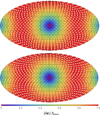 |
Fig. 1 Apparent shifts, δv, in source positions caused by the two polarisation components of a plane GW propagating towards the centre of the maps, i.e. the ‘+’ component (top) and ‘×’ component (bottom). The background colour encodes the magnitude of the shift, |δu |, in units of the maximum shift ∆max. This and all other full-sky maps use the Hammer-Aitoff projection in equatorial coordinates, with α = δ = 0 at the centre, north up, and α increasing from right to left. |
3 Imprint of the GW signal on a Gaia-like astrometric solution
We now go on to discuss how the astrometric effects of a GW described in the previous section might be seen in a Gaia-like astrometric solution. For this purpose, it is necessary to consider the specific way observations are made with a Gaia-like instrument, as well as their interplay with the model parameters in the astrometric solution. These interactions are in generally quite complicated and a full characterisation can only be obtained by means of numerical simulations, as described in the next sections. Under simplifying assumptions, theoretical predictions can nevertheless be derived for some of the interactions, which is the subject of this section.
3.1 Nature of Gaia-like observations
We considered astrometric observations from a scanning space observatory based on the principles of the ESA missions HIPPARCOS and Gaia, using simultaneous observations of sources in two fields of view (FoVs), separated by a large angle Γ (basic angle). The nominal basic angle is 106.5° for Gaia and 58° for HIPPARCOS. The instrument rotates in space according to a prescribed scanning law, with a rotation period of hours.
The two FoVs are called preceding and following according to the direction of the instrument’s rotation. The position of a source in each FoV at a certain time can be specified by two field angles measured from the centre of the field: the along-scan (AL) angle 𝑔, and the across-scan (AC) angle, h. We denote the field angles in the preceding FoV as 𝑔p, hp, and in the following FoV as 𝑔f, hf (cf. Fig. 1 and Sects. 2.1 and 2.2 of Butkevich et al. 2017).
The size of each FoV is of the order of 1 deg; thus, at the times of observation the field angles are always ≲ 10−2 rad in absolute value. To first order we can then neglect the finite size of the FoV and all the details of what happens when the source transits the FoV, effectively regarding the observations as instantaneous (cf. Sect. 4.4 of Butkevich et al. 2017). Any time-dependent variation (‘signal’) in the positions of sources on the sky then translates into corresponding changes (δ𝑔p, δhp) or (δ𝑔f, δhf) of their measured field angles at the respective times of observation. Neglecting the geometrical calibration of the detectors within each FoV, the accurately measured AL and AC field angles constitute the elementary astrometric observations of a Gaia-like instrument.
3.2 Global astrometric solution
Given the basic angle and the accurate attitude of the instrument at the moment of observation, the observed field angles can be transformed into an instantaneous position of the source on the sky. The astrometric parameters of the source can in principle be determined from a sequence of such positions. However, the accuracy with which the actual attitude and calibration of the instrument is known a priori is not sufficient for the astrometric accuracy to be achieved. Therefore, the attitude and calibration parameters must also be determined from the astrometric observations (self-calibration). Consistency among the various source, attitude, and calibration parameters is ensured by solving all of them together in a global least-squares solution, as described for Gaia in Lindegren et al. (2012). The residuals of the solution (the difference between the observed and fitted field angles) may then contain imprints of any unmodelled signal in the data, such as the astrometric effects of the GW.
Naively, we might think that the GW effect would remain practically unchanged in the residuals of the astrometric solution. However, as discussed in the literature (Klioner 2014; Butkevich et al. 2017; Klioner 2018), this is not the case. The two main reasons are (i) that part of any unmodelled signal is absorbed by the attitude parameters and (ii) that another part of the signal may be absorbed by the source parameters. A significant part of the GW signal does however remain in the residuals, provided that the period of gravitational wave, Pgw, is not considerably larger than the time span T of the astrometric data (see also Sect. 2 of Klioner 2018).
Part of the GW signal could also be absorbed by the calibration parameters, which, in turn, could modify the source and attitude parameters in the global solution. This interaction cannot easily be described in general terms, because the calibration model tends to be very specific to a given instrument and tailored to its behaviour. One exception is the calibration of a possible variation of the basic angle, which is briefly addressed below.
3.3 Interaction with attitude and basic angle determination
We consider an arbitrary perturbation of the observed stellar positions, namely, a smooth function δu(t, α, δ) of both the time and position on the sky. Examples of such perturbations are: (i) a global shift of all parallaxes; (ii) a large-scale distortion of the positions and proper motions; and (iii) the astrometric effects of a low-frequency GW.
Based on a generalisation of the pioneering work of Lindegren (1977), Klioner (2014) and Butkevich et al. (2017) described an important problem in this scenario. Thanks to the scanning law, which is also a smooth function of time, any such perturbation will produce smooth, time-dependent variations, δ𝑔p, δhp, δ𝑔f, and δhf, of the observed field angles. These variations are observationally indistinguishable from a certain time-dependent variation of the attitude parameters and of the basic angle. Specifically, Eq. (7) of Butkevich et al. (2017) shows that the AC components of a signal, described by δhf and δhp, as well as the average of the AL components, (δ𝑔f + δ𝑔p)/2, are equivalent to a certain change in the attitude. Because the attitude is determined as a free function of time, with a time resolution (of seconds) that is much higher than the rotation period (hours), these components of δu are completely absorbed by the attitude parameters. The remaining AL part of the signal is effectively equivalent to a variation of the basic angle, δΓ = δ𝑔f − δ𝑔p. This signal can influence the astrometric source parameters, be partially absorbed by the basic-angle calibration, or remain in the residuals of the astrometric solution, depending on the calibration model used in the astrometric solution. As mentioned earlier in this paper, the interaction with the calibration model cannot be discussed in general terms and, thus, it is neglected here.
This general mechanism applies in particular to the case of the astrometric signal produced by a GW. Therefore, we conclude that the AC components of the GW signal and the mean of the AL components in the two FoVs are absorbed, to first order, by the attitude as determined in the astrometric solution (see Lindegren et al. 2012 for the standard attitude model of Gaia). Only the differential AL effect δ𝑔f − δ𝑔p carries information about the GW signal, but even part of that may be absorbed by the source parameters and/or the model of basic-angle variations.
These theoretical expectations have been confirmed in dedicated numerical simulations (similar to those described in Sect. 4), in which only certain parts of a GW signal were used to compute the simulated data: only the AC part, only the AL part, only the mean AL signal in both FoVs, etc.
3.4 Interaction with astrometric source parameters
In the standard astrometric model of stellar motion (e.g. Sect. 3.2 of Lindegren et al. 2012), the motions of sources on the sky are described by five free parameters per source: two components of the position (α, δ), two components of the proper motion (µα*, µδ), and a parallax (ϖ). As explained above, the component of the GW signal that is not absorbed by the attitude parameters will partly alter the source parameters and partly remain in the residuals of the solution. In full generality, this interaction will be investigated below by means of the numerical simulations described in Sect. 4.
However, a simple model can elucidate the effect on the source parameters at least in the case of a GW with period Pgw sufficiently longer than the time span, T, covered by observations. In this case we assume that the effect on the parallax is negligible. A change of parallax would cause a periodic shift of the apparent position on the sky with a period equal to the orbital period of the observer (satellite) in its motion around the barycentre of the Solar System. For Gaia, this period is about one year. From Appendix A, we can see that a GW signal causes elliptic variations of the apparent positions with a period equal to that of the gravitational wave, Pgw . Therefore, if Pgw ≫ T ≫ 1 year, it is a plausible assumption that the effect of such a GW on parallax is negligible. This is explicitly justified by the simulations below.
Therefore, we only consider variations of positions ∆α*=  and
and  , and proper motions
  and
and  . Here,
  , and
, and  are the parameters computed under the influences of a GW signal, while α, δ, µα*, and µδ are the true ones or those computed with no GW signal in the observations. Here and below, the asterisk in α* indicates that the cos δ factor is implicit, as in
  .
.
We further assume that there is an infinite number of observations uniformly distributed over the time interval of observations t − t0 ∈ [− T/2, T/2], where t0 is the middle of the observational period and also the reference epoch of the catalogue (that is, the source positions are defined at t0). Now, we fit the GW effect δα*, δδ as given by Eq. (A.11) in Appendix A by the linear functions ∆α* + ∆µα* (t − t0) and ∆δ + ∆µδ (t −t0). The small Rømer correction −c−1 p⋅xobs(t) in Eq. (A.2) is ignored, so that the meaning of the strain and phase parameters  , and
, and  is defined by the reference epoch tref in Eq. (A.2). Without loss of generality we set tref = t0. We also neglect that a part of the GW signal is absorbed by the attitude parameters. Considering all the assumptions, standard linear regression then gives
 (1)
(1)
 (2)
(2)
where
 (3)
(3)
 (4)
(4)
and
 (5)
(5)
 (6)
(6)
These are the functions illustrated in Fig. 2, with the argument
 (7)
(7)
Here, θ is the angular distance between the direction of observation and the direction of propagation of the GW, given by Eq. (A.26), and R is the rotation matrix given by Eq. (A.27).
The residuals of this linear fit,
 (8)
(8)
have a zero mean. We can derive also the following result for the standard deviations of the residuals in AL and AC directions (σr,AL and σr,AC):
 (9)
(9)
where hc = |hc|, hs = |hs|, and  in agreement with Eq. (A.19).
It is seen that the effective change in position only depends on the cosine parameters  and
and  , while the proper motion is only affected by the sine parameters,
  and
and  . This is easily understood from the parity properties of the sine and cosine terms with respect to the reference epoch t0 = tref. The functions f(y) and 𝑔(y) depicted in Fig. 2 represent the averaging over the observations: a part of the elliptic motion described in Appendix A.2 is approximated by a straight line corresponding to a constant proper motion. The argument y is proportional to the ratio T/Pgw of the time span of the observations to the GW period. In the limit when Pgw ≫ T (small y), we have f(y) ≃ 1 and 𝑔(y) ≃ y, in which case, for a given set of strain parameters, the GW has maximal effect on the position, while the proper motion effect is proportional to the GW frequency ν = 1 /Pgw = y/(πT). The function 𝑔(y) reaches a maximum value of 1.3086 for y ≃ 2.0816, which corresponds to Pgw ≃ 1.5092 T. For a given amplitude of the strain parameters, the proper motion is therefore maximally sensitive to GW periods of about 1.5 times the observation interval.
The linear regression shown in Eqs. (1)–(7) can be reasonably applied for Pgw ≳ T, provided that T is considerably greater than the orbital period of the observer with respect to the barycentre of the Solar System. The latter orbital period drives the parallactic signal in the astrometric data. In this regime, we can expect that virtually the whole GW signal goes into the corresponding changes of the positions and proper motion, so that both the parallax and the residuals are only minimally affected. On the other hand, for y ≫ 1, one sees that the averaging functions f (y) and 𝑔(y) tend to zero, so that under the assumptions of this model, the effects of a GW of a higher frequency on positions and the proper motions gradually diminish. From the numerical simulations presented below, we find that significant changes in the positions and proper motions occur also for higher GW frequencies. This can be attributed to various complications neglected in the present analysis: the actual scanning law, the finite number of observations, the partial absorption of the GW signal by attitude parameters, and the interaction with parallax. For Pgw ≫ T, on the other hand, Fig. 4 shows that Eqs. (1)–(7) accurately describe the simulated variations of the astrometric parameters.
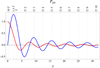 |
Fig. 2 Averaging functions f (y) and 𝑔(y) shown in red and blue, respectively. The equivalent GW period, Pgw = πT/y, is given on the top axis in terms of T, the time span of the observations. For fixed T = 5 yr, y is equivalent to the GW frequency ν = y/(πT) ≃ y × 2.017 nHz. |
4 Numerical simulations
The goal of the work presented here (and in the next section) is to reveal the typical characteristics of the influence of a GW on a Gaia-like astrometric solution for various GW parameters. To assess these effects, we used simulated data and computed the corresponding astrometric solution with realistic modelling of sources and attitude.
We used the AGISLab software (Holl et al. 2012) for the simulations. This software offers various options for simulating observations, computing the astrometric solution and exporting all kinds of parameters as well as the residuals of the solution. In particular, the software allows one to add arbitrary signals to the model used when generating the simulated observations and to omit or include random noise (photon noise) in the observations.
Using AGISLab, we simulated Gaia-like observations including a signal of a GW with some specific parameters, but without random observational noise. These observations are processed inside AGISLab, using standard models for the sources and the satellite attitude as described, for instance, in Lindegren et al. (2012). Because the standard models do not take into account any GW effects, the resulting astrometric solution directly shows the effect of the GW on the source parameters, spacecraft attitude, and solution residuals. We note that without the GW signal, such a solution gives zero residuals and reproduces the assumed model parameters to within the numerical precision of the computations, ~10−3 µas.
It is clear that the number of simulations required to exhaustively explore the seven-dimensional (7D) parameter space of a plane continuous GW is prohibitively large. For example, to cover possible GW source directions, with ≃10° spacing, requires about four hundred simulations for just a single GW frequency and a specific set of strain parameters. Instead, we selected GW parameters that are representative for a wide region of the parameter space to demonstrate the most important effects, both qualitatively and quantitatively.
The simulations cover GW periods ranging from Pgw = 30 yr (νmin ≃ 1.05627 nHz) to approximately 50.2 d with a fixed spacing in frequency of 1.5 nHz. This gives 154 frequency values with νmax = νmin + 153 × 1.5nHz ≃ 230.55627 nHz. Additionally, we incorporated five GW frequencies with periods between 100 yr and 5 yr to achieve a denser coverage in the low-frequency range, and the 11 special frequencies affecting positions and/or parallax listed Table 2 that are combinations of the fundamental frequencies of the scanning law (see Eq. (13)). Consequently, in total 170 GW frequencies were used. The rationale behind this choice of frequency interval is given in Appendix C.
For each frequency, we chose five different sets of strain parameters as follows:
We set all four parameters to the same value. This gives GWs with eccentricity e = 1 (see Eq. (A.17)).
We set
 and
and  to get GWs with e = 0.
We randomly select each strain parameter from the same uniform distribution. The resulting eccentricity, e, can have any value from 0 to 1, but higher values are considerably more probable.
We randomly choose the strain parameters in such a way that the eccentricity is approximately uniformly distributed from 0 to 1. This was done numerically, by first generating a very large number of combinations of random amplitudes, binning them by eccentricity, and then randomly selecting first an eccentricity bin, followed by one of the amplitude combinations within that bin.
The fifth set was generated exactly as the fourth, only using a different random seed. This set was added to reduce sampling noise, after it was found that the uniform distribution of eccentricity gives the largest variation in attitude errors and residual statistics.
These recipes define the strain parameters up to some normalising factor. Because the astrometric GW signal is linear in the strain parameters, the choice of normalisation factor is (in principle) arbitrary, as long as the resulting astrometric effects are considerably greater than the numerical noise in the astrometric solutions. We chose the normalisation that gives ∆max = 1 mas in every simulation. Although this implies unrealistically large values for the strain, it does not matter thanks to the linearity of the effect and because all numerical results are reported relative to ∆max.
For each set of frequency and strain parameters we randomly selected the GW propagation direction from a uniform distribution on the sky. This yielded 170 × 5 = 850 independent simulations that form the basis for the following investigations.
All simulations used (1) one million sources randomly distributed on the sky; (2) no observational noise; (3) the nominal Gaia instrument configuration; (4) the nominal Gaia scanning law; and (5) a mission duration of T = 5 yr. The reference epoch tref for the GW parameters (as in Eq. (A.2)) and that for the source parameters t0 were both chosen to be exactly in the middle of the simulated mission. The number of sources was selected in order to ensure a stable astrometric iterative solutions on the one side, and a sufficiently fine sampling of the astrometric GW effect in the solution on the other. We stress that the statistical characteristics of the GW effect in the solution as discussed in Sect. 5 are independent of the number of sources in the simulations.
In addition to these simulations, we made some additional simulations for specific GW parameters. These are used, for instance, to illustrate the distribution of astrometric errors on the sky (Fig. D.1), to give additional statistics for selected frequencies (Table D.1), and to discuss the effects of the GW phase for a very long period (Table 1). The technical setup for these simulations was the same as above, except for the specific GW parameters described in each case.
Errors induced by the different strain parameters in the low- frequency regime.
5 GW-induced errors in the astrometric solution
5.1 Overview of the numerical results
A main result of our simulations is that any injected GW signal, regardless of its frequency and other parameters, generates errors in the astrometric source parameters and in the spacecraft attitude, as well as in the residuals of the solution. How the errors are distributed in the various parts of the solution mostly depends on the GW frequency ν, or period Pgw = 1 /ν. For periods comparable to or greater than the duration of the data, Pgw ≳ T (subsequently referred to as the low-frequency regime), the positions and proper motions are altered most, while the residuals are barely affected. By contrast, in the high-frequency regime (Pgw ≲ T) all parts of astrometric solutions are affected. For some specific GW frequencies – those related to the fundamental frequencies of the scanning law – the astrometric errors are substantially larger than for nearby frequencies. At the same time, the errors in the attitude are significantly increased while the effect on the residuals is smaller. This shows that substantial parts of the GW signal are absorbed by the astrometric and attitude parameters for these specific GW frequencies. We also note that the errors in the astrometric parameters are not randomly distributed on the sky but display a variety of complex patterns.
In the following subsections, these findings are discussed in greater detail. Figures 5 and 6, summarising basic error statistics versus GW frequency, provide a useful reference for the discussion.
5.2 Low-frequency regime: Pgw ≳ T
The simulations for GWs with periods greater than the duration of observations (corresponding to ν ≲ 6.3 nHz for T = 5 yr) largely confirm the predictions of the simplified theoretical model in Sect. 3.4, namely that the source parameters in this frequency regime absorb most of the astrometric effects of the GW. This is most clearly seen in Fig. 3, which zooms in on the low-frequency end (ν < 15 nHz, or Pgw > 2.1 yr) of the standard deviations in Figs. 5 and 6. The errors in position and proper motion from the simulations behave qualitatively as expected, with maxima at roughly the frequencies where the theoretical curves in Fig. 2 have extrema, and minima where the theoretical curves go through zero. For example, the maximal errors in proper motions were predicted to appear at Pgw ≃ 1.5T = 7.5 yr in the simulations, which agrees very well with the maxima in the second panel of Fig. 3 (cf. Table 2, which puts the maximum at Pgw ≃ 7.2 yr as measured from the simulation results).
Moreover, the model (1)–(9) valid for any particular source allows one to compute a theoretical prediction of the normalised standard deviations of the GW effects in the position, proper motions and residuals of an astrometric solution involving many sources homogeneously distributed over the sky. Indeed, assuming that both components of positions (∆α* and ∆δ) and proper motions (∆µα* and ∆µδ) have the same standard deviations as well as considering that statistically in our simulations hc ≃  we get
 (10)
(10)
 (11)
(11)
where  is the averaged value of e2 in our simulations. These two theoretical curves are shown on two upper plots of Fig. 3. Then assuming that the residuals in AL and AC have the same standard deviations (so that σr,AL ≃ σr,AC) we get from Eq. (9)
 (12)
(12)
We remind that Eq. (12) is derived ignoring interaction of the GW signal with the attitude. Section 3.3 explains that the AC effects of the GW signal are fully absorbed by the AC attitude, while the AL effects are partially absorbed by the AL attitude and partially equivalent to a variation of the basic angle. Since we do not model any variation of the basic angle in our simulation, that second part remains in the AL residuals. The theoretical curve (12) is shown on the attitude plot on Fig. 3 where it reasonably agrees with the normalised standard deviation of the variations in AC attitude ∆X and ∆ Y. For the AL effects, we get  , where σ∆Z is the standard deviation of the AL attitude variations and σAL is the standard deviation of the AL residuals (shown on the two lowest plots of Fig. 3).
The theoretical model was derived with many simplifying assumptions, including that there would be no effect of the GW on the parallaxes and attitude. Figure 3 shows that there is some such effect at all frequencies, but that it becomes progressively smaller towards zero frequency. Figure 4 shows the errors of the astrometric parameters induced by a GW with a period of 20 yr. At this low frequency the errors in parallax are indeed negligible compared to the errors in the other parameters. The large-scale variations of the errors in position and proper motion shown here closely follow the predictions using Eqs. (1)–(7).
Equations (1)–(7) show that the effect of the GW on positions and proper motions in the low-frequency regime depends on the phase of the GW: only the cosine-related strain parameters  and
and  influence the positions, while only the sine-related parameters
  and
and  produce an effect in the proper motions. Also this aspect of the theoretical model in Sect. 3.4 has been confirmed by the dedicated simulations reported in Table 1. The table also shows the much smaller effect on parallax for Pgw ≫ T.
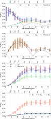 |
Fig. 3 Standard deviations of the errors in source parameters, attitude, and residuals, for GW periods longer than 2.1 yr. These plots are zoomed versions of the ones in Figs. 5–6, but with a few more points added to improve the coverage at the lowest frequencies. Theoretical curves shown on the three upper plots are given by Eqs. (10), (11), and (12), respectively (see text for further explanations). |
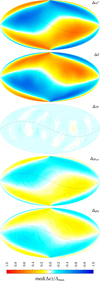 |
Fig. 4 Astrometric errors caused by a GW with Pgw = 20 yr (ν ≃ 1.58 nHz) propagating towards the centre of the maps with strain parameters |

5.3 High-frequency regime: Pgw ≲ T
From Fig. 5, we can see that GWs with periods shorter than the duration of observations, T, produce errors in the astrometric parameters with a typical standard deviation of 0.1−0.2∆max. At certain frequencies the errors do however reach much higher values, as discussed in Sect. 5.4. Averaged over all sources, the errors are typically small (less than ±0.01 ∆max), but again at specific frequencies they can be much larger. For the components of proper motion and for α the average error barely reaches ±0.1∆max, but for δ and ϖ it can reach ±0.3∆max. Generally, the average errors in right ascension are considerably smaller than in δ and ϖ. The reason for this anisotropy is not fully understood. Appendix D contains additional results from the simulations, illustrating the characteristics of the astrometric errors produced by GWs.
Figure 6 shows the standard deviations and average values of the attitude errors and residuals of the solution. The standard deviation of the attitude errors is typically 0.25–0.35∆max for the rotation around the nominal spin axis Z, corresponding to the AL attitude (see Sect. 3.1 of Lindegren et al. 2012 for the definition of the Scanning Reference System of Gaia), and 0.4– 0.7∆max around the other two axes X and Y, corresponding for the AC attitude. For some specific GW frequencies the standard deviation can reach 0.5∆max in Z (AL) and ≃1.0∆max for X and Y (AC). The average errors are typically close to zero, but can reach ±0.4∆max for the rotation around the Y axis.
Concerning the residuals shown in the lower panels of Fig. 6, it can be noted that the average values (bottom right) are always very small, within ±0.0002∆max. Corresponding to the peaks in the astrometric and/or attitude errors, the residuals (bottom left) show decreased standard deviations at the same frequencies. The most prominent example is seen around a GW period of approximately 96.1 d.
Based on the theoretical model in Sect. 3.3 we expect the AC attitude (around the X and Y axes) to absorb the entire AC signal of a GW, while the AL attitude (around Z) only absorbs the mean of the AL signals in the two FoVs. This behaviour is largely confirmed by the standard deviations of the residuals shown in the bottom left panel of Fig. 6: whereas the standard deviation of the AL residuals is significant (0.25–0.45∆max), that of the AC residuals is much smaller (0.04–0.07∆max). The standard deviation of the AL residuals can be compared to the standard deviations given of the full GW signal given in Table B.1 as 0.4–0.6∆max. We can see that the AL residuals only contain a part of the total GW signal. That the standard deviation of the AC residuals is not completely negligible can be attributed to the simplifying assumptions adopted in the theoretical model. One such assumption was that second-order (differential) effects within the FoV, caused by the finite FoV size, can be neglected. But this can only explain a minor part of the AC residuals, of the order of 0.01 ∆max. Instead, the dominating contribution to the AC residuals comes from the interaction between source and attitude parameters that was also neglected in the theoretical model.
To cross-check our understanding of these interactions, a series of dedicated simulations were made in which only specific components of the GW signal were added to the observations. For example, if the AL components (δ𝑔f , δ𝑔p) of the GW signal were included, but not the AC components (δhf , δhp), it was found that the source parameters did not change from a reference simulation including all four AL and AC components of the GW signal. If, on the other hand, the AC components were included together with the mean value of the AL components (so the signal  was applied in both FoVs), the attitude errors were found to be the same as in the reference simulation, while the source parameters were virtually unaffected by the applied signal, resulting in very small AL and AC residuals. Two important results from these experiments are (i) that errors in the source parameters are caused almost exclusively by the differential AL component of the GW signal, δ𝑔f − δ𝑔p ; (ii) that these source errors in turn produce residuals in both coordinates, although they are much smaller (by a factor ∼5) AC than AL. The first result is expected based on the simplified model of Sect. 3.3. The second result can only be understood by considering the way the attitude and source parameters are determined in the global astrometric solution by minimising the sum of squared residuals (SSR). As detailed e.g. in Eq. (24) of Lindegren et al. (2012), both AL and AC observations are used, so SSR = SSRAL + SSRAC. Although there is an attitude that fit the AC observations perfectly also in the presence of the GW signal (corresponding to SSRAC = 0 in the present noise-free simulations), a somewhat different attitude may be preferred in terms of the total SSR, if it allows a slight reduction of the AL residuals.
Even though parts of the GW signal are absorbed by the source and attitude models, the AL residuals generally contain a large fraction of the AL component of a high-frequency GW signal. This is illustrated in Fig. 7, showing an arbitrary short segment of the data from one of the simulations. It is seen that the residuals Rp in the preceding FoV approximately follow the curve giving half the differential GW signal, (δ𝑔p − δ𝑔f)/2. For the full dataset the correlation coefficient is 0.92 in this example. The residuals in the following field (not shown in the plot) similarly follow half the differential GW signal, but with the opposite sign. It should be noted that the actual GW signal in that FoV (δ𝑔p), shown by the black curve, is not well reproduced by the residuals (correlation coefficient 0.72). The simulations also show that the AC residuals have no correlation with the AC component of the GW signal.
Another way to look at the astrometric errors is to consider the errors in position, and separately the ones in proper motion as a vector field on the sphere. For each star, the errors in positions or proper motions have a direction and a magnitude, given by either the combination of errors ∆α* and ∆δ, or ∆µα* and ∆µδ, respectively. The errors in parallax ∆ϖ can be considered as a scalar field on the sphere. Then one can consider the RMS of those vector or scalar fields. However, this way would not give any new information compared to what we have above. Indeed, for any n-dimensional vector x the components of which are to be investigated we have a simple relation between the RMS value (rx), the standard deviation (σx) and the average values  . Since we have already considered the standard deviations and averages of the astrometric errors, there is no reason to consider also the RMS of the corresponding scalar and vector fields.
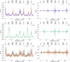 |
Fig. 5 Statistics of the errors of the astrometric source parameters versus the frequency of the injected GW. Left: standard deviations of the errors. Right: averages of the errors. Top to bottom: errors in position (α and δ), parallax (ϖ), and proper motion (µα* and µδ). All statistics are normalised to the maximum astrometric amplitude of the GW effect, ∆max . The coloured bars show the range of statistics obtained in the five simulations for each frequency (see Sect. 4); for improved visibility the coloured lines connect the average statistics in the corresponding bars. The red tick marks on both lower and upper horizontal axes of the left pictures show the positions of the GW frequencies and periods shown in Table 2. |
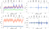 |
Fig. 6 Statistics of the attitude errors (top) and astrometric residuals (bottom) versus the frequency of the injected GW. Left: standard deviations of the errors or residuals. Right: averages of the errors or residuals. In the upper panels, A in ∆A is a placeholder for X, Y, or Z, the three axes of the Scanning Reference System (Sect. 3.1 of Lindegren et al. 2012). Similarly, in the lower panels, R is a placeholder for the residual along-scan (AL), across-scan in the preceding FoV (ACp), or across-scan in the following FoV (ACf). The coloured bars show the range of statistics obtained in the five simulations for each frequency (see Sect. 4); for improved visibility the coloured lines connect the average statistics in the corresponding bars. The standard deviations of the residuals in ACp and ACf virtually coincide. |
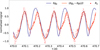 |
Fig. 7 Example of the GW signal from one of the simulations and how it appears in the astrometric solution. The black curve (δ𝑔p) is the AL component of the GW signal in the preceding FoV. The red dots (Rp) show the AL residuals of the solution in the same FoV. For comparison, the red curve shows half the differential GW effect, (δ𝑔p − δ𝑔f)/2. All data are normalised by ∆max. The frequency of the GW signal was ν = 101.160 nHz, equivalent to a period of Pgw ≃ 114.42 d. |
5.4 Frequency bands of special significance
A striking feature of Figs. 5 and 6 is the multitude of peaks in the standard deviations of the astrometric and attitude errors, and sometimes also in the average errors. As Fig. 6 shows, there is an increase in the AC attitude errors at some of these frequencies, accompanied by a decrease mainly in the AL residuals. We have verified that the peaks occur at the same frequencies independent of the direction of propagation of the GW.
Most of the peaks are approximately centred on GW frequencies that can be expressed as
 (13)
(13)
for small integer numbers k, l, and m. Here, ν1yr ≃ 31.688 nHz corresponds to a period of 1 yr ≡ 3.15576 × 10⁷ s, νSL ≃ 183.791 nHz corresponds to the precession period 1 yr/5.8 ≃ 62.97 d of the scanning law, and νT is a frequency depending on the duration T of the mission, with νT ≃ 4.4 nHz for T = 5 yr, corresponding to a period of about 7.2 yr. The dimensionless constant 0.694 appearing in the expression for νT is further discussed below.
Table 2 lists the most prominent peaks in the standard deviations of the errors in position, parallax, and proper motion, as measured from the data displayed in Fig. 5. Peaks were detected by fitting a template profile to the data in a sliding window of width 15 nHz, using a cosine-squared profile with a full width at half maximum (FWHM) of 7.5 nHz. This was done separately for the position, parallax, and proper motion data, but combining the components in α and δ for the position and proper motion data for improved signal-to-noise ratio. Each peak corresponds to a local maximum in the amplitude of the fitted profile.
Table 2 also shows our interpretation of the peaks in terms of k, l, and m (using νT = 4.4 nHz), and the differences between the measured peak frequency and νk,l,m from Eq. (13). In two cases the interpretation is ambiguous, as discussed below. Considering the frequency discretisation and the scatter in the standard deviations at each frequency point, the agreement between the measured and calculated frequencies is quite good.
It is noted that for the position and parallax errors, the peaks always have m = 0, while for the proper motion errors the peaks tend to come in pairs around the peaks in position error, with m = ±1. One apparent exception is the peak in proper motion errors at 51.1 nHz, tentatively identified as ν−4,1,−1 = 52.6 nHz: no corresponding peak was detected in position errors at the expected frequency ν−4,1,0 = 57.0 nHz, although there is one in parallax errors. However, the data do not rule out a small peak around 57.0 nHz in the position errors, blended with the much stronger peak at 63.6 nHz (see the top-left panel of Fig. 5). If this interpretation is correct, there should also be a peak in the proper motion errors at ν−4,1,1 = 61.4 nHz, which however would be blended with the strong peak at 59.6 nHz. The nearly coinciding theoretical frequencies ν2,0,−1 = 59.0 nHz and ν−4,1,1 = 61.4 nHz is not the only example of an ambiguous identification; the peak at 123.9 nHz, in the table identified as ν−2,1,1 = 124.8 nHz, could just as well be be ν−4,0,−1 = 122.4 nHz. One more potentially ambiguous identification is the peak at 29.0 nHz, in the table identified as ν−5,1,1 at 29.8 nHz. This peak could in principle be a blend with ν1,0,−1 at 27.3 nHz, but because neither ν1,0,0 at 31.7 nHz is seen in the position data, nor ν1,0,1 at 36.1 nHz in the proper motion data, we conclude that the peak is probably not a blend.
The peaks in position and parallax errors can be qualitatively understood as an interference phenomenon between the GW signal and the characteristic frequencies ν1yr and νSL of the scanning law, or their overtones. When the GW frequency is close to kν1yr + lνSL for some k and l, the beat frequency ∆ν = ν − kν1yr − lνSL will be in the low-frequency regime (|∆ν| ≲ 1 /T) and large position and/or parallax errors may be created by the same mechanism as described in Sect. 3.3. We then expect the peaks in position and parallax errors to have a FWHM equal to that of the function f (y) (considering both positive and negative y), or 1.2067/T ≃ 7.6 nHz in reasonable agreement with the simulation results.
That the peaks in the proper motion errors are offset by ±νT ≃ ±4.4 nHz from the corresponding peak in the position errors can also be understood in the framework of the theoretical model of Sect. 3.3. According to Eqs. (1)–(7), the effect in proper motion scales as the derivative of the effect in position with respect to the GW frequency: 𝑔(y) = −3df /dy. Assuming that this relation holds also for the beat signal1, we expect the peaks in proper motion errors to occur at the frequencies where |ց(∆ν)| has a maximum, that is with an offset of ±0.6626/T from the corresponding peak in position errors. Theoretically, then, the numerical constant in Eq. (13) should be 0.6626 rather than the value 0.694 estimated from the simulations. We note that the low-frequency peak shown in the second panel of Fig. 3 can formally be identified with ν0,0,1 , as suggested by the first entry in Table 2. Numerical simulations for a mission duration of T = 3 yr confirm that the width of the peaks and the offset of the peaks in proper motion both scale as 1/T.
An in-depth investigation of the mechanisms producing the increased errors in position and/or parallax around the specific frequencies listed in Table 2 is beyond the scope of this paper. For example, we have no explanation why some combinations of k and l affect both positions and parallaxes, and others only one of them, or why there are peaks at νk,0,0 for k = 1, 2, 3, 4, and 6, but apparently not for k = 5 (at ν5,0,0 = 158.4 nHz). We note that there are similarities with the spurious periods that may be detected in astrometric and photometric time series of Gaia data purely as a result of the scanning law. That phenomenon was extensively investigated by Holl et al. (2023), and indeed their Eq. (3) is equivalent to our Eq. (13) for m = 0. Clearly, the specific distribution of scanning angles and observation times for a given source allows the source model to absorb a larger fraction of the GW signal for certain frequencies. As shown in Appendix D, the sky distributions of the astrometric errors for GW signals close to one of the special frequencies νk,l,0 (e.g. Pgw = 1 yr, 96.1 d, 76.1 d, 63.0 d, and 53.7 d) display characteristic large-scale patterns, not present for other frequencies. Similar patterns were discussed by Holl et al. (2023).
5.5 Sky distribution of the errors
The statistical description of the astrometric errors in previous sections does not say anything about how the errors are distributed on the sky. Examples of their sky distributions are shown in Fig. D.1 of Appendix D. One sees that the distributions crucially depend on the GW frequency. At some GW frequencies and for some of the parameters, the maps display large-scale patterns in which the median astrometric error per pixel can be as high as ≃1.2∆max. As noted earlier, this happens at the specific frequencies discussed in Sect. 5.4, while at other frequencies the spatial features have smaller angular scales and smaller amplitudes. At all frequencies, however, the spatial distributions are strongly non-random.
Although the instantaneous astrometric effect (δα*,δδ) of a GW is dominated by its quadrupole component (Book & Flanagan 2011; Klioner 2018), the errors induced in the astrometric parameters rarely have a quadrupole spatial distribution. Clearly, the intricate interaction between the GW signal, astrometric model, and method of observation (where part of the signal is absorbed by the attitude) results in very complicated patterns of the astrometric errors on the sky.
In order to provide a more comprehensive description of the spatial distributions, we analyse the GW-induced parallax errors in terms of (scalar) spherical harmonics (SH), and the vector fields of the errors in position and proper motion in terms of vector spherical harmonics (VSH; Mignard & Klioner 2012). Generally speaking, SH and VSH of a given degree ℓ quantify the strength of the scalar or vector field at a typical angular scale of ≃180o/ℓ.
For each simulation we fit the SH and VSH expansions up to degree ℓmax = 20 separately for the errors in parallax, position, and proper motion. For a specific SH or VSH degree ℓ, the RMS value of the error pattern is computed as
 (14)
(14)
where Pℓ is the power of the SH components of degree ℓ for the parallax errors, and the sum of the toroidal  and spheroidal
  powers of the VSH components for the errors in position and proper motion (see Sect. 5.2 of Mignard & Klioner 2012). We note that Rℓ is rotationally invariant and therefore independent of the coordinate system used (e.g. equatorial, ecliptic, or galactic).
Figure 8 shows the mean Rℓ/∆max obtained in the simulations as a function of the GW frequency and ℓ. The peaks at various GW frequencies, already seen in Fig. 6, are easily recognised, but now we can also see how those errors are distributed in spatial frequency (ℓ). These diagrams confirm and further quantify the general conclusions drawn from the sky maps, namely that the predominantly quadrupole (ℓ = 2) nature of the GW signal does not translate into predominantly quadrupole components in the error patterns. Instead, much of the power is found in higher- degree harmonics, typically 4 ≲ ℓ ≲ 10, although lower degrees (1 ≤ ℓ ≤ 3) dominate in the frequency bands with enhanced astrometric errors, where ℓ = 3 is often the strongest component. It is seen that the parallax errors can have a considerable dipole (ℓ = 1) contribution, and even some global offset (ℓ = 0) at certain frequencies. For the proper motion errors, the distribution in ℓ mirrors that of the position errors, after taking into account the frequency splitting by m = ± 1.
In the VSH expansion of the errors in position and proper motion, the toroidal components of degree ℓ = 1 represent a global rotation of the reference frame, and the spheroidal components of degree ℓ = 1 represent a form of distortion known as glide (Mignard & Klioner 2012). As implemented in AGISLab, the astrometric solution is set up in such a way that the resulting positions and proper motions have no net rotation with respect to their initial values (in our case the true values). Any global rotation in the source errors caused by the GW signal, if present, is hence removed by the astrometric solution, and the toroidal components of degree ℓ = 1 should therefore be zero for position and proper motion errors. However, technical differences in the way these computations are made within AGISLab and in our external VSH analysis result in non-zero rotation components in our VSH coefficients2. Those rotations are small and can be ignored in the discussion below.
The situation is different for the glide, corresponding to the spheroidal components of degree ℓ = 1 in the position and proper motion errors: these components are not removed by the astrometric solution. Following the conventions in Mignard & Klioner (2012) and Gaia Collaboration (2021), the glide is here represented by a vector 𝑔, given by Eq. (6) of the latter reference in terms of the spheroidal VSH components of degree ℓ = 1. The ICRS components of 𝑔 are therefore directly obtained from the VHS expansion of the errors. However, a glide in the proper motion errors caused by a GW cannot be distinguished from the glide a/c caused by the acceleration a of the solar system barycentre. Measuring a is one of interesting results of Gaia-like global astrometry (Gaia Collaboration 2021), and a relevant question then is how much glide might be produced by GWs. Figure 9 shows the magnitude of the glide |𝑔| in position and proper motion, normalised to ∆max. For low-frequency GWs (Pgw ≳ T), the glide in position as well as in proper motion is small compared to the effect at higher frequencies. This is expected because the GW model expressed in VSH has no coefficients at degree ℓ = 1 (Klioner 2018) and the GW signal at these frequencies goes almost unaltered to the source errors, as discussed in Sect. 3.4. For GWs of higher frequency (Pgw ≲ T), the glide in both position and proper motion is stronger, up to ~0.25∆max. But while the acceleration of the solar system barycentre produces a pure glide (with no VSH components of degree ℓ > 1), it is evident from Fig. 8 that the glide component produced by a GW in the proper motions is only a minor part of the total GW effect at that frequency. For real Gaia measurements, the expected GW amplitudes and their astrometric effects are small and, therefore, the glide effect generated by them is negligible for the studies of the solar system acceleration. (The glide in position does not seem to have any physical meaning, but is included in Fig. 9 for completeness and because it is relevant for understanding the peaks in the proper motion diagram.)
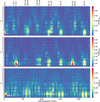 |
Fig. 8 Normalised RMS variation Rℓ/∆max of the SH/VSH expansion of the astrometric errors in position (top), parallax (middle), and proper motion (bottom), displayed versus GW frequency for degrees ℓ ≤ 20. Equivalent data are shown by the solid lines in Figs. E.1–E.3 (see Appendix E for details). |
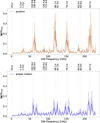 |
Fig. 9 Absolute values of the glide 𝑔 introduced by a GW in positions (upper panel) and proper motions (lower panel) of the astrometric sources. The coloured bars show the range of values obtained in the five simulations for each frequency (see Sect. 4); for improved visibility the coloured lines connect the average statistics in the corresponding bars. The glide is computed from the spheroidal VSH coefficients of degree ℓ = 1 as described in Sect. 6 of Gaia Collaboration (2021). In our case, with negligible frame rotation in the data, the total glide is |𝑔| = (3/2)1/2 R1. |
6 Concluding remarks
In Appendix A, we present a new theoretical formulation of the astrometric effects of a plane GW. While this is mathematically equivalent to previously published models, the new formulation permits a simple geometrical interpretation of the effects: to an astrometric observer, the GW signal appears as a synchronised elliptical motion of all sources on the sky. The eccentricity of the ellipses is the same for all sources and depends only on the strain parameters, while the size and orientation of the ellipses also depend on the celestial position of the source relative to the propagation direction of the GW. A useful insight from this formulation is that the astrometric effects of a GW resemble, to a certain extent, the effects of astrometric binaries, but with the important difference that the GW affects all sources on the sky in a highly coordinated manner. The resulting pattern of motions for many millions of sources potentially makes a global astrometric survey mission, such as Gaia, a sensitive detector of GWs.
The detectability of the GW signal depends not only on the properties of the GW and the accuracy of the astrometric measurements, but also on the specific conditions under which the measurements are made. For example, it is clear from the description above that all astrometric sources within a small area of the sky are very similarly affected by the GW. Differential measurements in a small field of view are therefore not sensitive to the GW effects, whereas global or wide-angle astrometry might be.
In this paper, we analyse the effects of a plane GW with constant frequency and strain parameters on a Gaia-like astrometric solution. We argue (Sect. 3) that the GW signal, such as any global smooth astrometric signal, is observationally equivalent to certain time-dependent modifications of the attitude and basic angle of the instrument. It is only the latter (basic-angle like) component of the GW signal that is potentially observable. However, depending on the frequency of the GW, that component could also be partly or fully absorbed by the astrometric solution in the form of (very small but systematic) errors in the positions, proper motions, and parallaxes of the astrometric sources. For the vast majority of sources (ordinary stars), these errors are undetectable because the true (unperturbed) values of the astrometric parameters are not known to sufficient accuracy. It is only for sources at cosmological distances (quasars) that we might presume to know the true proper motions and parallaxes. The part of the basic-angle like component that is not absorbed by the astrometric source parameters creates systematic patterns in the residuals that are, at least in principle, possible to detect also for ordinary stars.
In Sect. 3.4, we provide an analytical model for the astrometric errors in positions and proper motions, as well as the astrometric residuals, for GWs in the low frequency regime (Pgw ≳ T). This simple model, supported by simulations in this frequency range (Sect. 5.2), is particularly relevant for the search of GW signals in the proper motions of quasars. Previously, the general assumption has been that GW signals with such low frequencies would manifest themselves solely as systematic patterns in the quasar proper motions. However, we find that this is not the case. The position parameters can also absorb major parts of the signal depending of the phase of the GW. Even more importantly, the magnitude of the GW-induced effects in proper motions (and positions) depends on the GW frequency, even for Pgw ≳ T . The analytical model defines the sensitivity function for the study of primordial GWs using quasar astrometry. On the other hand, we find that also in this regime part of the GW signal remains in the residuals. This may allow one to use not only the quasar proper motions, but also the astrometric residuals of ordinary stars to search for GWs with Pgw ≳ T.
As explained in Sect. 4, we have performed a large number of numerical simulations with a realistic Gaia-like observational setup, using the simulation software AGISLab (Holl et al. 2012). The GW periods investigated by simulations range from Pgw = 100 yr to ≃ 50 d. The reasoning behind this choice of GW periods is explained in Appendix C. The simulations demonstrate the complicated character of the GW-induced errors in a Gaia-like astrometric solution, as discussed in some detail in Sects. 5 and 5.5 and in Appendices D and E. In particular, our simulations show that a significant part of the GW signal is absorbed by the astrometric source parameters (positions, proper motions, and parallaxes) even for GWs with periods considerably shorter than the time span of observations.
Although the GW-induced astrometric errors in general cannot be detected (except possibly for quasars), they are nevertheless interesting for understanding the fundamental limits of astrometric missions. The simulations described here, covering a wide range of GW parameters and assuming a realistic observational setup, can be used to estimate the astrometric noise floor set by the expected GW background (GWB) in the relevant frequency ranges. As demonstrated, for instance, in Agazie et al. (2024) and references therein, the recent pulsar timing results show that the GWB likely exists. This GWB may represent a fundamental limit for future astrometric projects aiming at much higher accuracy than Gaia. Both the detectability of the GWB using astrometry and the accuracy limits imposed by it will be discussed elsewhere.
In this study, we focus on the effects of individual GW sources that may possibly be detected by astrometry. Perhaps the most important finding from our simulations is the fact that, for all frequencies with Pgw ≲ T , a significant part of the GW signal remains in the residuals of the astrometric solution. This strengthens our belief that a GW signal, if present at a sufficient amplitude, could be detected by a posterior analysis of the residuals in the standard astrometric solution. This is a very interesting and important task. A separate publication will be devoted to the formulation and demonstration of a dedicated GW search algorithm in astrometric data, and specifically in Gaia data.
Some important aspects of the GW search algorithms can be gleaned already from the present analysis. The residual curves in Fig. 6 imply that the sensitivity function for astrometric searches of GW with Pgw ≲ T is not flat. At frequencies where the (normalised) astrometric errors are larger and the residuals smaller, the possibility to detect the GW signal is correspondingly reduced. As discussed in Sect. 5.4, this happens in particular around the GW frequencies related to the scanning law. Depending on the position on the sky, the temporal sampling of the sources allows the astrometric model to absorb a greater or smaller part of the GW signal. This could have important implications for the design of a GW search algorithms based on the residuals: at certain GW frequencies, the astrometric residuals from certain parts of the sky provide little or no information on a possible GW signal.
Considerations in Appendix C allow us to draw another important conclusion concerning the GW search algorithm, namely that it should not assume constant GW frequency over the whole observational period. That assumption was expedient and revealing in the present study, but in a search algorithm it would effectively preclude the detection of possible GW sources with chirp masses above a certain limit, as illustrated in Fig. C.1. This topic will be further discussed elsewhere.
A theoretical limit for the sensitivity of Gaia to a GW signal can be derived from the total astrometric weight of the mission, ω, calculated by summing up the astrometric weights of the individual AL measurements (Eq. (62) in Lindegren et al. 2012).
With respect to forthcoming Gaia DR4 data we estimate ωGDR4 ≃ 2 × 10⁶ µas−2 if the ≃ 1012 residuals of all sources with full astrometric solutions are used3. From the bottomleft diagram in Fig. 6 and considering Eq. (A.32), we have σR ≃ 0.36∆max ≃ 0.15h (with 〈e2〉 ≃ 8/15 in the simulations). The minimum detectable strain at the 1σ level is therefore h ≳ ω−1/2/0.15 ≃ 2 × 10⁻¹⁴. Taking into consideration that the GW model has seven parameters and that the GW solution may include additional nuisance parameters, the actual theoretical limit may be higher by a significant factor.
Data availability
Appendices D and E are available as online supplementary material on Zenodo at https://doi.org/10.5281/zenodo.14773103.
Acknowledgements
This work is financially supported by ESA grant 4000115263/15/NL/IB and the German Aerospace Agency (Deutsches Zentrum für Luft- und Raumfahrt e.V., DLR) under grants 50QG1402 and 50QG2202. We also thank the Center for Information Services and High Performance (ZIH) at TU Dresden for providing a considerable amount of computing time. The work by LL is supported by the Swedish National Space Agency. Various software products produced by the Gaia DPAC were used in this work and are gratefully acknowledged. This especially concerns the AGISLab framework which was developed by Berry Holl, David Hobbs, Alex Bombrun and other Gaia DPAC members. We also express our gratitude to Hagen Steidelmüller, who has maintained and continued the development of AGISLab for many years and implemented additional special features used for this project. Finally, we also thank Enrico Gerlach, Jan Meichsner and Sven Zschocke for fruitful discussions.
Appendix A Model for the astrometric effects of a plane GW
In this appendix we provide a concise description of the model for the astrometric effect of a GW and show that it results in an apparent elliptical motion of every source on the sky.
A.1 Basic formulae
A plane continuous GW with constant frequency is completely described by seven parameters: αgw and Δgw defining the direction of propagation, the GW frequency ν and the four strain parameters  , and
, and  encoding the strains and phases of the two polarisations (we follow here Jaranowski & Krolak 2009). As presented by Klioner (2018), the astrometric effect Δu at the point u (|u | = 1) with coordinates (a, Δ) can be written
 (A.1)
(A.1)
where
 (A.2)
(A.2)
 (A.3)
(A.3)
 (A.4)
(A.4)
 (A.5)
(A.5)
 (A.6)
(A.6)
 (A.7)
(A.7)
 (A.8)
(A.8)
 (A.9)
(A.9)
 (A.10)
Here, t is the time of observation, xobs (t) the barycentric position of the observer at the moment of observation, and the phases of the strain parameters are defined with respect to the reference epoch tref .
The Rømer correction −c−1 p · xobs(t) in Eq. (A.2) reflects the fact that the GW phase Φ at the location of observer is offset from the GW phase 2πv(t − tref) at the solar system barycentre. The Rømer correction is numerically small (≲ 500 s at the position of the Earth of Gaia), and can often be neglected in theoretical considerations.
P is the rotation matrix between the reference system in which the gravitational wave propagates in the +z direction, and the celestial reference system in which the propagation direction is p .
The dimensionless strain parameters  , and
, and  describe the magnitude of the astrometric effects of the GW. In the astrometric context they are conveniently expressed in angular units (e.g. mas or µas).
We remind that the model described here depends only on the gravitational field of a GW at the observer. As discussed for example in Book & Flanagan (2011) and Klioner (2018), one can completely ignore the ‘source term’, that is, the effect depending on the GW at the astrometric sources.
Finally, we note that Eq. (A.1) describes the variation of the observable direction towards an astrometric source as seen by an observer at position xobs (t) and having zero velocity relative to the Barycentric Celestial Reference System (BCRS; Soffel et al. 2003). The corresponding direction observed by an observer moving relative to the BCRS can be computed using the usual relativistic aberration formulas, for example Eq. (10) of Klioner (2003).
A.2 Elliptic motion on the sky caused by a GW
The model above can be written in a way that gives an important insight into the nature of the effect, namely that the astrometric effect of a GW consists of coordinated elliptic motions of all sources on the sky. We can derive the following simple representation of the GW effect:
 (A.11)
 (A.12)
 (A.13)
where matrix D is detailed below, and the vector
 (A.14)
describes an ellipse with semi-major axis a, semi-minor axis b, eccentricity e and position angle ϕ (counted from the positive ’horizontal’ axis defined by eα to the major axis):
 (A.15)
 (A.16)
 (A.17)
 (A.18)
 (A.19)
 (A.20)
 (A.21)
 (A.22)
 (A.23)
 (A.24)
One can show that 0 < 𝒮 < 1 and, therefore,  and
and  . For ℬ = 0 and h× = h+ one gets a circle with
  and undefined ϕ.
The matrix D in Eq. (A.11) is obtained as
 (A.25)
where
 (A.26)
is the angle (0 ≤ θ ≤ π) between the direction of observation (α, Δ) and the direction of GW propagation (αgw , Δgw), and R is the rotation matrix
 (A.27)
 (A.28)
 (A.29)
 (A.30)
with Δα = α − αgw. The matrix R is orthogonal with det R = 1, so that ℱ2 + 𝒢2 = 𝒩2. The signs of ℱ and 𝒢 are non-trivial and necessitate the explicit formulas for both ℱ and 𝒢 given above. When using the formulas for R, special care must be taken when θ is close of 0 or π. For θ = 0 and θ = π we have D = 0, while R is undefined.
The astrometric effect of the GW can therefore be described as an apparent elliptic motion of the source in the plane of the sky, with semi-major axis
 (A.31)
eccentricity e, and orientation defined by a combination of the angle ϕ (which depends only on the strain parameters) and the rotation matrix R (which depends only on the position of the source and the direction of GW propagation). Here a, e, ϕ, θ, and R are given respectively by Eqs. (A.15), (A.17), (A.18), (A.26), and (A.27).
The eccentricity of the ellipse is the same for all sources, and the period of the effect equals the GW period Pgw = ν−1. Depending on the ratio T/Pgw, the whole ellipse or only part of it is observed (here T is the mission duration). The unperturbed position of the source is at the centre of the ellipse and the motion is such that the phase angle is almost linear with time, Φ ≃ 2πν(t −tref). The Rømer correction to the phase in Eq. (A.2) results in a small perturbation of the position of the source along the ellipse, depending also on the direction of GW propagation ( p).
Figure A.1 depicts the positional offsets over time for ten randomly selected astrometric sources at different celestial positions. For each source the effect is plotted in the respective local plane coordinates Δα* (along eα) and ΔΔ (along eΔ). The rotation and scaling of the different ellipses, caused by R and  sin θ, are clearly seen.
From Eq. (A.31) it is seen that the maximal amplitude of the astrometric effect for a given GW,
 (A.32)
is reached for sources located normal the direction of GW propagation (sin θ = 1). From Eq. (A.15) we have Δmax ≤ h/2.
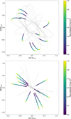 |
Fig. A.1 Positional offsets of ten randomly chosen astrometric sources, as produced by two GWs propagating in the same direction and having the same frequency, but with different strain parameters |


Appendix B Statistical properties of the GW-induced signal
This Appendix gives some analytical results concerning the statistical properties of the astrometric GW signal itself, ignoring its possible interaction with the astrometric solution (as discussed in Sect. 3). We are specifically interested in the statistics of Δu · s, where Δu is the instantaneous GW signal for a source at position u, and s is a unit vector in the tangent plane of the sky at u (so u · s = 0). In the context of Gaia, s could be the AL or AC direction for a particular observation of the source, in which case Δu · s is the AL or AC component of the GW signal at the source. The problem becomes analytically tractable by considering a random time of observation (and hence a random phase Φ of the GW), a random propagation direction of the GW, and a randomly selected direction s. By disregarding a number of incidental factors, such as the scanning law and the phase of the GW, the resulting statistics are conveniently suited for comparison with the error statistics of the astrometric solution, and especially its residuals.
In Appendix A we demonstrated that |Δu | ≤ ∆maxThe normalised shift
 (B.1)
(B.1)
therefore lies between −1 and +1. Using Eqs. (A.11), (A.14), (A.25), and (A.32) we find that the normalised shift can be written κ = r(Φ)sin θ cos φ, where r(Φ) = |b |/a, θ is the angle between the direction of GW propagation and the source, and φ is the angle between the vectors s and Δu. As before, Φ is the GW phase, b is the vector given by Eq. (A.14) and a is the semi-major axis given by Eq. (A.15).
The distribution of κ = r(Φ) sin θcos φ is derived as follows. Using that cos θ is uniformly distributed in [−1,1], and that φ is uniformly distributed in [0, 2π), we see that the factor sin θcos φ is uniformly distributed in [−1,1]. Concerning r(Φ), we find from Eq. (A.14) that it can be written as
 (B.2)
(B.2)
where e is the eccentricity given by Eq. (A.17), and the phase shift ψ/2 is defined by
 (B.3)
(B.3)
 (B.4)
(B.4)
We note that  for any strain parameters. Because the phase Φ is uniformly distributed in [0,2π), the constant phase shift ψ/2 in the right member of Eq. (B.2) obviously plays no role for the distribution of r(Φ): Φ and Φ − ψ/2 (modulo 2π) are both uniformly distributed in [0, 2π). Combining the above results, we find that the probability density function (PDF) of κ for |κ| ≤ 1 reads
 (B.5)
(B.5)
where 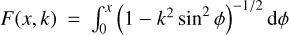 is the (incomplete) elliptic integral of the first kind and K(k) = F(π/2, k) is the complete elliptic integral of the first kind. (For |κ| > 1 we obviously have PDFκ = 0.) To derive Eq. (B.5) one needs to use several results and properties of the elliptic integrals, given e.g. in Byrd & Friedman (1971) and Erdélyi et al. (1953).
Equation (B.5) demonstrates one very important result, namely that under the given assumptions of random sampling, the distribution of κ only depends on e. In particular, it does not depend on either the GW direction or the GW frequency. From Eqs. (A.15) and (A.32) it is then seen that the distribution of Δu · s only depends on e and the total strain h.
Equations (B.3)–(B.5) become degenerate for e = 0; but in that case r(Φ) ≡ 1, so κ is uniformly distributed in [−1,1]. More generally, for a given 0 ≤ e ≤ 1, κ is uniformly distributed for  and falls off quite fast outside this interval. The distribution is clearly symmetric around κ = 0. Therefore, both the mean value and the skewness of κ are zero. The standard deviation of κ is obtained by computing the corresponding integral of Eq. (B.5), yielding
 (B.6)
(B.6)
By a similar analytical computation, the excess kurtosis of κ is found to be  . The unnormalised projected signal Δu · s has zero mean and standard deviation
  .
.
In the case of Gaia, the above statistics derived for the random sampling are valid for either the AL and AC components of the GW signal; the only difference would be in the interpretation of the angle ϕ. The standard deviation in Eq. (B.6) nicely agrees with the results of Sect. 5.2, namely that the GW signal is distributed between the source parameters, as in Eqs. (10)–(11), and the corresponding residuals, as in Eq. (12).
These theoretical results are confirmed by numerical simulations. We generated 6 × 10⁶ AL signal values. The GW frequency was set to 200 nHz, a random GW direction on the sky was taken, and the nominal Gaia scanning law was used with 5 years of observations. The distribution of the simulated values for four values of the eccentricity is depicted in Fig. B.1 and summary statistics are given in Table B.1. The small differences between the analytical model and the simulation results can be explained by the use of a single GW direction in the simulations and the specific sampling by the Gaia scanning law, which is not completely random.
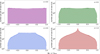 |
Fig. B.1 Histograms of the normalised projections κ = Δu · s/Δmɑx of the GW signal for different values of the eccentricity e. The filled bar charts represent the AL signal components in Gaia observations simulated as described in the text. The lines show the corresponding distributions from the analytical formula in Eq. (B.5). |
Statistics of the astrometric GW signal for different eccentricities.
Notes. The table gives the statistics listed in the first column of the quantity κ defined by Eq. (B.1). Four different eccentricities, e, of the GW signal are considered, as indicated in the top row. Values in the columns marked Theory are computed using the model distribution in Eq. (B.5). Values in the columns marked Num are computed from numerical simulations as described in the text. Qp (p = 0.01, 0.05, …, 0.99) denotes the p-th quantile. All statistics are rounded to two decimal places.
Appendix C Relevant GW frequency range
In this study we primarily consider a GW frequency range from approximately 0.317 nHz to ≃231 nHz, corresponding to periods between 100 yr and 50.2 d. Here we present and discuss the rationale for this choice.
The lower frequency bound, corresponding to a maximum GW period of 100 yr, is related to the mission duration, taken to be T = 5 yr. From the discussions in Klioner (2018) and in Sects. 3.4 and 5.2 of this paper, it is clear that an increasing fraction of the GW signal is absorbed by the astrometric parameters for Pgw ≳ T . According to Eqs. (12) and (B.6) that fraction, in terms of signal variance, exceeds 0.997 for Pgw = 25T. Although that limit is somewhat arbitrary, there is obviously not much point in considering even longer periods.
The choice of upper frequency limit is also somewhat arbitrary, but based on several practical and theoretical considerations. One purely practical thing is that the amount of computations required for the numerical simulations increases in direct proportion to the maximal GW frequency. Thus, it is desirable not to choose an upper limit higher than motivated by other requirements. On the other hand, it is desirable to include, with some margin, the special frequency νSL ≃ 184.000 nHz related to the Gaia scanning law, discussed in Sect. 5.4. A third requirement follows from the expected properties of supermas- sive black hole binaries that could generate GWs of sufficiently stable frequencies, and which are strong enough to be potentially detectable with Gaia. The rest of this Appendix is an attempt to quantify this requirement.
One of the limitations of the present study is that the GW frequency is assumed to be constant throughout the length of the mission. We consequently want to avoid considering cases where the GW from an inspiralling binary system demonstrates considerable frequency drift during the period of observation T = 5 yr. Section 8 of Klioner (2018) contains a brief discussion of the GW parameters expected from such binary systems, based on Buonanno (2007) and Jaranowski & Krolak (2009).
One of the limitations of the present study is that the GW frequency is assumed to be constant throughout the length of the mission. Since we are thus only interested in the regime where the GW frequency is changing very slowly, it is sufficient to consider the post-Newtonian theory. We also ignore alternative theories to General Relativity. Equation (59) of Klioner (2018) then gives a differential equation for the evolution of the GW frequency from a binary on a circular orbit. Integrating this formula from the initial frequency ν0 at time t0 gives
![Mathematical equation: $v(t) = {\left[ {v_0^{ - 8/3} - {{{2^8}{\pi ^{8/3}}} \over {5{c^5}}}{{(G{\cal M})}^{5/3}}\left( {t - {t_0}} \right)} \right]^{ - 3/8}} = {v_0}{(1 - Sx)^{ - 3/8}},$](/articles/aa/full_html/2025/03/aa53545-24/aa53545-24-eq104.png) (C.1)
(C.1)
where ℳ is the chirp mass of the binary and
 (C.2)
(C.2)
 (C.3)
(C.3)
Requiring that the relative change of the GW frequency over the mission, (ν(t0 + T) − ν0)/ν0, does not exceed є then leads to an upper limit on the chirp mass,
 (C.4)
(C.4)
where M⊙ is the mass of the Sun and Pgw0 = 1/ν0. Using Eq. (57) of Klioner (2018) now gives the maximal possible strain h created by a GW source at the (luminosity) distance r:
 (C.5)
(C.5)
For a given maximal relative change є of the GW frequency, Eqs. (C.4) and (C.5) give the maximal allowed chirp mass ℳ and the maximal expected strain as functions of the initial GW period Pgw0 and other parameters. From Eq. (60) of Klioner (2018) we note that
 (C.6)
(C.6)
equals T/τ, where τ is the time to coalescence (at t0 + τ). In the regime of interest here we have S << 1 or T << τ.
From the point of view of data processing the relative frequency change є may not be the most interesting quantity. In this study we have assumed a GW of constant frequency, and a more relevant quantity is then the coherence of the phase over the mission; in other words, how much the actual phase Φ(t) deviates from the best-fitting linearly varying phase  . The true phase is defined by the differential equation dΦ/dt = 2πν(t) and the initial condition Φ(t0) = Φ0 . Integrating Eq. (C.1) gives
 (C.7)
(C.7)
where, for small Sx, the phase dilation factor in large brackets equals  . In the linear approximation it can be shown that the condition
 (C.8)
(C.8)
where ϱ is the maximal phase error in radians, is equivalent to a maximal relative change in frequency
 (C.9)
(C.9)
or
 (C.10)
This є can be used in Eqs. (C.4) and (C.5) to derive the maximal chirp mass and maximal expected strain for a given maximal phase error ϱ in the constant frequency model.
Figure C.1 shows the maximal chirp mass and the maximal expected strain as functions of the GW period for three different values of ϱ. The duration of the observations is taken to be T = 5yr and a minimal plausible distance r = 100 Mpc is assumed. For a maximal phase error of ϱ = 1 rad, we find that Pgw = 50 d gives a maximal strain slightly below 10−14, roughly compatible with the theoretical sensitivity of Gaia DR4 as discussed in Sect. 6 (see also Sect. 7 of Klioner 2018 for a related earlier discussion). This justifies not considering shorter periods than Pgw ≃ 50 d in the present study, where the GW is assumed to have negligible frequency drift over 5 yr.
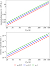 |
Fig. C.1 Top: Maximal chirp mass ℳ of a binary system for which the assumption of a constant GW frequency Pgw gives a maximal phase error of ϱ = 0.25, 0.5, and 1 rad over the duration of observations T = 5 yr (circular orbit assumed for the binary). Bottom: Maximal strain h under the same conditions, assuming a luminosity distance of r= 100 Mpc. |
References
- Agazie, G., Antoniadis, J., Anumarlapudi, A., et al. 2024, ApJ, 966, 105 [NASA ADS] [CrossRef] [Google Scholar]
- Bini, D., & Geralico, A. 2018, Phys. Rev. D, 98, 124036 [Google Scholar]
- Book, L. G., & Flanagan, É. É. 2011, Phys. Rev. D, 83, 024024 [NASA ADS] [CrossRef] [Google Scholar]
- Braginsky, V. B., Kardashev, N. S., Polnarev, A. G., & Novikov, I. D. 1990, Nuovo Cimento B Ser., 105, 1141 [Google Scholar]
- Buonanno, A. 2007, arXiv e-prints [arXiv:0709.4682] [Google Scholar]
- Butkevich, A. G., Klioner, S. A., Lindegren, L., Hobbs, D., & van Leeuwen, F. 2017, A&A, 603, A45 [NASA ADS] [CrossRef] [EDP Sciences] [Google Scholar]
- Byrd, P. F., & Friedman, M. 1971, Handbook of Elliptic Integrals for Engineers and Physicists, 2nd edn. (Berlin–Heidelberg–New York: Springer-Verlag) [Google Scholar]
- Çalışkan, M., Chen, Y., Dai, L., et al. 2024, J. Cosmology Astropart. Phys., 2024, 030 [Google Scholar]
- Darling, J., Truebenbach, A. E., & Paine, J. 2018, ApJ, 861, 113 [NASA ADS] [CrossRef] [Google Scholar]
- Erdélyi, A., Magnus, W., Oberhettinger, F., & Tricomi, F. 1953, Higher Transcendental Functions, Volume II (New York-Toronto-London: McGraw-Hill Book Company, Inc.) [Google Scholar]
- Gaia Collaboration (Prusti, T., et al.) 2016, A&A, 595, A1 [NASA ADS] [CrossRef] [EDP Sciences] [Google Scholar]
- Gaia Collaboration (Klioner, S. A., et al.) 2021, A&A, 649, A9 [EDP Sciences] [Google Scholar]
- Gaia Collaboration (Klioner, S. A., et al.) 2022, A&A, 667, A148 [NASA ADS] [CrossRef] [EDP Sciences] [Google Scholar]
- Gaia Collaboration (Vallenari, A., et al.) 2023, A&A, 674, A1 [NASA ADS] [CrossRef] [EDP Sciences] [Google Scholar]
- Gwinn, C. R., Eubanks, T. M., Pyne, T., Birkinshaw, M., & Matsakis, D. N. 1997, ApJ, 485, 87 [Google Scholar]
- Holl, B., Lindegren, L., & Hobbs, D. 2012, A&A, 543, A15 [NASA ADS] [CrossRef] [EDP Sciences] [Google Scholar]
- Holl, B., Fabricius, C., Portell, J., et al. 2023, A&A, 674, A25 [NASA ADS] [CrossRef] [EDP Sciences] [Google Scholar]
- Jaranowski, P., & Krolak, A. 2009, Analysis of Gravitational-Wave Data (Cambridge University Press) [Google Scholar]
- Kaiser, N., & Jaffe, A. 1997, ApJ, 484, 545 [NASA ADS] [CrossRef] [Google Scholar]
- Klioner, S. A. 2003, AJ, 125, 1580 [Google Scholar]
- Klioner, S. A. 2004, Phys. Rev. D, 69, 124001 [Google Scholar]
- Klioner, S. A. 2014, Velocity error and effective basic angle calibration (VBAC): basic principles and possible applications, Tech. Rep. GAIA-C3-TN-LO-SK- 020, available from the Gaia document archive: https://dms.cosmos.esa.int/cs/livelink?objId=3268461 [Google Scholar]
- Klioner, S. A. 2018, Class. Quant. Grav., 35, 045005 [Google Scholar]
- Kopeikin, S. M., Schäfer, G., Gwinn, C. R., & Eubanks, T. M. 1999, Phys. Rev. D, 59, 084023 [NASA ADS] [CrossRef] [Google Scholar]
- Lindegren, L. 1977, Thermal stability and the determination of parallaxes, Tech. rep., Lund Observatory, available from https://doi.org/10.5281/zenodo.7642744 [Google Scholar]
- Lindegren, L., & Bastian, U. 2010, in EAS Publications Series, 45, eds. C. Turon, F. Meynadier, & F. Arenou, 109 [NASA ADS] [CrossRef] [EDP Sciences] [Google Scholar]
- Lindegren, L., Lammers, U., Hobbs, D., et al. 2012, A&A, 538, A78 [NASA ADS] [CrossRef] [EDP Sciences] [Google Scholar]
- Mignard, F., & Klioner, S. 2012, A&A, 547, A59 [NASA ADS] [CrossRef] [EDP Sciences] [Google Scholar]
- Mihaylov, D. P., Moore, C. J., Gair, J. R., Lasenby, A., & Gilmore, G. 2018, Phys. Rev. D, 97, 124058 [Google Scholar]
- Moore, C. J., Mihaylov, D. P., Lasenby, A., & Gilmore, G. 2017, Phys. Rev. Lett., 119, 261102 [Google Scholar]
- O’Beirne, L., & Cornish, N.J. 2018, Phys. Rev. D, 98, 024020 [Google Scholar]
- Pyne, T., Gwinn, C. R., Birkinshaw, M., Eubanks, T. M., & Matsakis, D. N. 1996, ApJ, 465, 566 [NASA ADS] [CrossRef] [Google Scholar]
- Soffel, M., Klioner, S. A., Petit, G., et al. 2003, AJ, 126, 2687 [Google Scholar]
Two remarks should be made concerning the applicability of this relation. (i) Although Eqs. (1)–(7) were derived for a continuum of observations uniformly distributed over the time span of observations, the model can readily be generalised for an arbitrary finite sequence of discrete observations, but the effects in proper motion are still proportional to the derivative of the effects in position with respect to ν. (ii) The effects in position and proper motion depend on different strain parameters, and are therefore in principle independent of each other. Statistically speaking, however, the magnitudes of the effects are still expected to follow this relation.
In both AGIS and AGISLab the so-called Frame Rotator is configured to fit only toroidal components of order ℓ = 1, whereas our external VHS analysis fits all VSH harmonics up to ℓmax = 20. Moreover, the Frame Rotator takes into account the correlations between the α and δ components of the positions or proper motions and uses a special algorithm for outlier rejection, whereas the present VSH analysis ignores correlations and assumes no outliers. A detailed description of the Frame Rotator algorithm can be found in Appendix E of Gaia Collaboration 2022.
We note that the astrometric weight of an individual source strongly depends on the properties of that source (e.g. its magnitude). Therefore, the total astrometric weight is not a simple function of the number of sources but crucially depends on various characteristics of the entirety of observational data.
All Tables
All Figures
|
Fig. 1 Apparent shifts, δv, in source positions caused by the two polarisation components of a plane GW propagating towards the centre of the maps, i.e. the ‘+’ component (top) and ‘×’ component (bottom). The background colour encodes the magnitude of the shift, |δu |, in units of the maximum shift ∆max. This and all other full-sky maps use the Hammer-Aitoff projection in equatorial coordinates, with α = δ = 0 at the centre, north up, and α increasing from right to left. |
| In the text | |
|
Fig. 2 Averaging functions f (y) and 𝑔(y) shown in red and blue, respectively. The equivalent GW period, Pgw = πT/y, is given on the top axis in terms of T, the time span of the observations. For fixed T = 5 yr, y is equivalent to the GW frequency ν = y/(πT) ≃ y × 2.017 nHz. |
| In the text | |
|
Fig. 3 Standard deviations of the errors in source parameters, attitude, and residuals, for GW periods longer than 2.1 yr. These plots are zoomed versions of the ones in Figs. 5–6, but with a few more points added to improve the coverage at the lowest frequencies. Theoretical curves shown on the three upper plots are given by Eqs. (10), (11), and (12), respectively (see text for further explanations). |
| In the text | |
|
Fig. 4 Astrometric errors caused by a GW with Pgw = 20 yr (ν ≃ 1.58 nHz) propagating towards the centre of the maps with strain parameters |
| In the text | |
|
Fig. 5 Statistics of the errors of the astrometric source parameters versus the frequency of the injected GW. Left: standard deviations of the errors. Right: averages of the errors. Top to bottom: errors in position (α and δ), parallax (ϖ), and proper motion (µα* and µδ). All statistics are normalised to the maximum astrometric amplitude of the GW effect, ∆max . The coloured bars show the range of statistics obtained in the five simulations for each frequency (see Sect. 4); for improved visibility the coloured lines connect the average statistics in the corresponding bars. The red tick marks on both lower and upper horizontal axes of the left pictures show the positions of the GW frequencies and periods shown in Table 2. |
| In the text | |
|
Fig. 6 Statistics of the attitude errors (top) and astrometric residuals (bottom) versus the frequency of the injected GW. Left: standard deviations of the errors or residuals. Right: averages of the errors or residuals. In the upper panels, A in ∆A is a placeholder for X, Y, or Z, the three axes of the Scanning Reference System (Sect. 3.1 of Lindegren et al. 2012). Similarly, in the lower panels, R is a placeholder for the residual along-scan (AL), across-scan in the preceding FoV (ACp), or across-scan in the following FoV (ACf). The coloured bars show the range of statistics obtained in the five simulations for each frequency (see Sect. 4); for improved visibility the coloured lines connect the average statistics in the corresponding bars. The standard deviations of the residuals in ACp and ACf virtually coincide. |
| In the text | |
|
Fig. 7 Example of the GW signal from one of the simulations and how it appears in the astrometric solution. The black curve (δ𝑔p) is the AL component of the GW signal in the preceding FoV. The red dots (Rp) show the AL residuals of the solution in the same FoV. For comparison, the red curve shows half the differential GW effect, (δ𝑔p − δ𝑔f)/2. All data are normalised by ∆max. The frequency of the GW signal was ν = 101.160 nHz, equivalent to a period of Pgw ≃ 114.42 d. |
| In the text | |
|
Fig. 8 Normalised RMS variation Rℓ/∆max of the SH/VSH expansion of the astrometric errors in position (top), parallax (middle), and proper motion (bottom), displayed versus GW frequency for degrees ℓ ≤ 20. Equivalent data are shown by the solid lines in Figs. E.1–E.3 (see Appendix E for details). |
| In the text | |
|
Fig. 9 Absolute values of the glide 𝑔 introduced by a GW in positions (upper panel) and proper motions (lower panel) of the astrometric sources. The coloured bars show the range of values obtained in the five simulations for each frequency (see Sect. 4); for improved visibility the coloured lines connect the average statistics in the corresponding bars. The glide is computed from the spheroidal VSH coefficients of degree ℓ = 1 as described in Sect. 6 of Gaia Collaboration (2021). In our case, with negligible frame rotation in the data, the total glide is |𝑔| = (3/2)1/2 R1. |
| In the text | |
|
Fig. A.1 Positional offsets of ten randomly chosen astrometric sources, as produced by two GWs propagating in the same direction and having the same frequency, but with different strain parameters |
| In the text | |
|
Fig. B.1 Histograms of the normalised projections κ = Δu · s/Δmɑx of the GW signal for different values of the eccentricity e. The filled bar charts represent the AL signal components in Gaia observations simulated as described in the text. The lines show the corresponding distributions from the analytical formula in Eq. (B.5). |
| In the text | |
|
Fig. C.1 Top: Maximal chirp mass ℳ of a binary system for which the assumption of a constant GW frequency Pgw gives a maximal phase error of ϱ = 0.25, 0.5, and 1 rad over the duration of observations T = 5 yr (circular orbit assumed for the binary). Bottom: Maximal strain h under the same conditions, assuming a luminosity distance of r= 100 Mpc. |
| In the text | |
Current usage metrics show cumulative count of Article Views (full-text article views including HTML views, PDF and ePub downloads, according to the available data) and Abstracts Views on Vision4Press platform.
Data correspond to usage on the plateform after 2015. The current usage metrics is available 48-96 hours after online publication and is updated daily on week days.
Initial download of the metrics may take a while.