| Issue |
A&A
Volume 695, March 2025
|
|
|---|---|---|
| Article Number | A236 | |
| Number of page(s) | 13 | |
| Section | Interstellar and circumstellar matter | |
| DOI | https://doi.org/10.1051/0004-6361/202453196 | |
| Published online | 21 March 2025 | |
Erosion of a dense molecular core by a strong outflow from a massive protostar
1
Academia Sinica Institute of Astronomy and Astrophysics,
No. 1, Sec. 4, Roosevelt Road,
Taipei
10617,
Taiwan
2
Instituto Argentino de Radioastronomía (CCT-La Plata, CONICET; UNLP; CICPBA),
C.C. No. 5, 1894, Villa Elisa,
Buenos Aires,
Argentina
3
Institut de Ciencies de l’Espai (ICE-CSIC), Campus UAB, Carrer de Can Magrans S/N,
08193
Cerdanyola del Valles, Catalonia,
Spain
4
Institut d’Estudis Espacials de Catalunya (IEEC),
c/ Gran Capità, 2-4,
08034
Barcelona,
Spain
5
Instituto de Astronomía, Universidad Nacional Autónoma de México (UNAM),
Apartado Postal 70-264,
DF 04510
México,
Mexico
6
Departament de Física Quàntica i Astrofísica (FQA), Universitat de Barcelona (UB),
c/ Martí i Franquès 1,
08028
Barcelona,
Spain
7
Institut de Ciéncies del Cosmos (ICCUB), Universitat de Barcelona (UB),
c/ Martí i Franquès 1,
08028
Barcelona,
Spain
8
Instituto de Radioastronomía y Astrofísica, Universidad Nacional Autónoma de México,
Apartado Postal 3-72,
58089
Morelia, Michoacán,
Mexico
★ Corresponding author; This email address is being protected from spambots. You need JavaScript enabled to view it.
Received:
28
November
2024
Accepted:
24
February
2025
Abstract
Context. Molecular outflows from massive protostars can impact the interstellar medium in different ways, adding turbulence on different spatial scales, dragging material at supersonic velocities, producing shocks and heating, and physically impinging onto dense structures that may be harboring other protostars.
Aims. We aim to quantify the impact of the outflow associated with the high-mass protostar GGD 27-MM2(E) on its parent envelope and how this outflow affects its environment.
Methods. We present Atacama Large Millimeter/submillimeter Array Band 3 observations of N2H+ (1–0) and CH3CN (5–4), as well as Band 7 observations of the H2CO molecular line emissions from the protostellar system GGD 27-MM2(E). Through position–velocity diagrams along and across the outflow axis, we studied the kinematics and structure of the outflow. We also fit extracted spectra of the CH3CN emission to obtain the physical conditions of the gas. We use the results to discuss the impact of the outflow on its surroundings.
Results. We find that N2H+ emission traces a dense molecular cloud surrounding GGD 27-MM2(E). We estimate that the mass of this cloud is ~13.3–26.5 M⊙. The molecular cloud contains an internal cavity aligned with the H2CO-traced molecular outflow. The outflow, also traced by CH3CN, shows evidence of a collision with a molecular core (MC), as indicated by the distinctive increases in the distinct physical properties of the gas such as the excitation temperature, column density, line width, and velocity. This collision results in an X-shaped structure in the northern part of the outflow around the position of the MC, which produces spray-shocked material downstream in the north of MC, as observed in position–velocity diagrams both along and across the outflow axis. The outflow has a mass of 1.7–2.1 M⊙, a momentum of 7.8–10.1 M⊙ km s−1, a kinetic energy of 5.0–6.6×1044 erg, and a mass-loss rate of 4.9–6.0×10⁻⁴ M⊙ yr−1.
Conclusions. The molecular outflow from GGD 27-MM2(E) significantly perturbs and erodes its parent cloud, compressing the gas of sources such as the MC and ALMA 12. The feedback from this powerful protostellar outflow helps maintain the turbulence in the surrounding area.
Key words: stars: formation / stars: winds, outflows / ISM: clouds / ISM: jets and outflows
Deceased on November 19, 2024.
© The Authors 2025
 Open Access article, published by EDP Sciences, under the terms of the Creative Commons Attribution License (https://creativecommons.org/licenses/by/4.0), which permits unrestricted use, distribution, and reproduction in any medium, provided the original work is properly cited.
This article is published in open access under the Subscribe to Open model. This email address is being protected from spambots. You need JavaScript enabled to view it. to support open access publication.
1 Introduction
Protostellar jets and bipolar outflows typically emerge during the early stages of star formation, when a cold, dusty envelope starts to gather material into a disk. High accretion rates during this phase quickly lead to the formation of a central core, which will evolve into a protostar (e.g., Blandford & Payne 1982; Pudritz & Norman 1983; Bally 2016; Maureira et al. 2017). The protostellar jets represent the fast and collimated wind launched from the inner region of the disk, while the bipolar outflows are the material dragged by the jet or by the outflowing stellar wind (e.g., Snell et al. 1980). They have previously been classified as either a wide-angle disk wind or a jet-driven wind (see, e.g., Lee et al. 2000, 2001).
Despite the traditional theoretical expectation that outflows are bipolar, well-behaved structures (which is backed by a plethora of observations), there are several cases that do not follow this rule. There have been detections of monopolar outflows (e.g., Fernández-López et al. 2013; Stanke et al. 2022; Takaishi et al. 2024), outflows with multiple collimated ejections in different directions (e.g., Cunningham et al. 2009; Soker & Mcley 2013; Kwon et al. 2015; Takaishi et al. 2024; Sai et al. 2024), precessing jets and outflows (Marti et al. 1993; Anglada et al. 2007; Teixeira et al. 2008; Arce et al. 2013; Zapata et al. 2013), and, more recently, even detections of their spiraling streamlines using maser emission (Moscadelli et al. 2022, 2023).
Outflows play an important role in shaping the chemical and physical properties of star-forming regions. They can induce changes in the chemical composition of their host clouds by dragging molecules formed in the disk or stellar atmosphere (e.g., Bachiller 1996), and by producing new molecules as a result of collisions between the outflow with the cloud, or between outflows themselves (e.g., Zapata et al. 2018; Toledano-Juárez et al. 2023). Additionally, outflows contribute enough energy and momentum to maintain the turbulence (e.g., Plunkett et al. 2015), even though outflow feedback has a minor contribution compared to the gravitational potential energy of the clump.
Moreover, while it is common to see shocks produced in the internal working surfaces of protostellar outflows due to differences in, for instance, the ejection velocity, shocks can also occur when outflows collide with dense obstacles such as protostellar cores, a dense pocket of gas, and the walls of molecular clouds, or even when the outflows collide with each other (e.g., Hartigan et al. 1987; Raga et al. 2002; Zapata et al. 2018). When the obstacle encountered is smaller than the cross section of the outflow, it becomes entrained and a reverse bow shock is formed (a socalled cloudlet shock; e.g., Hartigan et al. 1987, 2000; Raga & Wang 1994). Alternatively, when the obstacle is larger, the outflow can be deflected, forming a quasi-stationary shock at the point of collision followed by a spray of shocked outflow material downstream (e.g., Raga et al. 2002). Despite the ubiquity of jets and outflows in the Galaxy, only a few have been confidently reported as deflected or colliding (e.g., Zapata et al. 2018; López et al. 2022).
The high-mass star-forming region GGD 27 is located in the dark molecular cloud L291 in the Sagittarius arm at a distance of 1.4 kpc (Añez-López et al. 2020). The (sub)millimeter emission in this region is dominated by two protostars, MM1 and MM2 (Girart et al. 2018). The massive MM1 protostar drives the spectacular radio jet associated with HH 80–81 (e.g., Rodríguez & Reipurth 1989; Marti et al. 1993; Carrasco-González et al. 2012; Masqué et al. 2012, 2015). This study focuses on MM2, which comprises two massive dust cores and disks – MM2(E) and MM2(W), also called ALMA 17 and ALMA 13 – which are apparently in a very early stage of evolution with masses of 1.9 ± 0.2 and 1.7 ± 0.3 M⊙, respectively (Fernández-López et al. 2011a,b). Busquet et al. (2019) estimate the lower limit of their disk masses to be 0.2 and 0.02 M⊙, and their radii 120 and 30, respectively. MM2(E) seems to be powering at least two molecular outflows: a SiO monopolar outflow due northeast and a CO bipolar precessing outflow oriented in a north–south direction (Fernández-López et al. 2013; Bally & Reipurth 2023). Qiu & Zhang (2009), based on line emission from high-density tracers such as CH3OH, CH3CN, ![Mathematical equation: $\[\mathrm{H}_2^{13} \mathrm{CO}\]$](/articles/aa/full_html/2025/03/aa53196-24/aa53196-24-eq7.png) , OCS, and HNCO, reported the existence of the source’s molecular core (MC), located 3″ north of MM2(E), along the path of the northern lobe of MM2(E)’s outflow. This source has no (sub)millimeter or infrared counterpart but presents a very rich shock-like chemistry, which may be indicative of a stationary shock between the outflow and a dense pocket of molecular gas (Fernández-López et al. 2011b). There is yet another faint and compact dust core about 5″ north of MM2(E). Finally, Kurtz & Hofner (2005) detected emission from H2O masers at the position of MM2(E) that displayed a very broad range of blueshifted velocities (reaching −100 km s−1; see also Martí et al. 1999). Also, Kurtz et al. (2004) reported a class I CH3OH maser spot about 1″ south of the MC source, in the range +12 to +16 km s−1.
, OCS, and HNCO, reported the existence of the source’s molecular core (MC), located 3″ north of MM2(E), along the path of the northern lobe of MM2(E)’s outflow. This source has no (sub)millimeter or infrared counterpart but presents a very rich shock-like chemistry, which may be indicative of a stationary shock between the outflow and a dense pocket of molecular gas (Fernández-López et al. 2011b). There is yet another faint and compact dust core about 5″ north of MM2(E). Finally, Kurtz & Hofner (2005) detected emission from H2O masers at the position of MM2(E) that displayed a very broad range of blueshifted velocities (reaching −100 km s−1; see also Martí et al. 1999). Also, Kurtz et al. (2004) reported a class I CH3OH maser spot about 1″ south of the MC source, in the range +12 to +16 km s−1.
This paper focuses on the molecular emission and kinematics associated with the northern redshifted lobe of the outflow from MM2(E). Section 2 details the observations. The results are presented in Sect. 3 and analyzed and discussed in Sect. 4. Finally, the conclusions are given in Sect. 5.
Spectral lines.
2 Observations
2.1 3 mm observations
Observations of the GGD 27 system were carried out with the Atacama Large Millimeter/submillimeter Array (ALMA) in Band 3 on 2014 June 27 as part of the program 2012.1.00441.S (PI: Roberto Galván-Madrid) during the Early Science Cycle 1 phase. In this work we focused on the emission of the hyperfine structure of the N2H+ (1–0) and the CH3CN (5–4) K-ladder lines. The calibrated data delivered by the ALMA European Regional Center were further self-calibrated and cleaned using Common Astronomy Software Application (CASA) package (CASA Team et al. 2022) version 6.4.0–16. A robust factor of 0.5 was applied to balance sensitivity and angular resolution and generate the molecular line cubes. Details of the rest frequencies, synthesized beam, spectral channel, and rms noise level are provided in Table 1.
2.2 1 mm observations
ALMA observations were obtained in Band 7 on 2016 September 6 and 7 as part of the program 2015.1.00480.S (PI: Josep Miquel Girart) during Cycle 3 phase. The observations were reported in detail in Fernández-López et al. (2023). The H2CO (41,3−31,2) line was included in the spectral window 27. This molecular transition was the only one in the spectral setup displaying significant emission associated with the main outflows originated by MM2(E). The data were calibrated using the CASA package version 4.7. Standard calibration and self-calibration using the continuum emission were applied to the spectral data. A robust factor of 0.5 to weigh the visibilities was applied to generate the H2CO (41,3−31,2) channel maps. Details of the observations of this line are presented in Table 1.
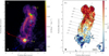 |
Fig. 1 GGD 27–MM2(E) molecular line emission of H2CO. (a) ALMA moment zero or integrated intensity map. (b) ALMA first moment or intensity-weighted velocity map. The two red arrows represent the redshifted NE and NW CO outflow directions, while the blue arrow is the blueshifted SE CO outflow direction Fernández-López et al. (2013). Yellow crosses represent the position of the continuum sources reported by Busquet et al. (2019): sources 13 and 17 are MM2(W) and MM2(E), respectively. The cyan dot and square mark the position of the CH3OH and H2O maser sources obtained from Kurtz et al. (2004) and Kurtz & Hofner (2005), respectively. The green star represents the position of the source MC taken from Qiu & Zhang (2009). The dashed black X-shaped curve and the dashed black line in (b) outline the shocked region around the MC and the outflow axis, while the dotted lines labeled C1–C9 indicate the position where the PV diagram presented in Fig. 4 was extracted. The synthesized beam is shown in the lower-left corner. The contour levels in both panels start at 5σ and are in steps of 3σ, 6σ, 9σ, and 12σ, where σ = 9.5 mJy beam−1 km s−1. |
3 Results
3.1 Morphology and kinematics of the outflow from MM2(E)
Figure 1 displays the emission of the H2CO molecular line associated with the source GGD 27-MM2(E). The ALMA moment zero or integrated intensity map is shown in Fig. 1a, while the ALMA first moment or intensity-weighted velocity map is presented in Fig. 1b. The maps are integrated over a velocity range of 4–21 km s−1 (the systemic velocity of the MM2(E) is ~11.5 km s−1). The emission of the H2CO extends up to ~![Mathematical equation: $\[4^{\prime\prime}_\cdot8\]$](/articles/aa/full_html/2025/03/aa53196-24/aa53196-24-eq8.png) (6720 au) northwest of the main source (P.A.≈
(6720 au) northwest of the main source (P.A.≈ ![Mathematical equation: $\[-14^{\circ}_\cdot5\]$](/articles/aa/full_html/2025/03/aa53196-24/aa53196-24-eq9.png) ), and it could be associated with the inner part of the CO molecular outflow previously reported by Fernández-López et al. (2013). Given that the observed H2CO line is a relatively dense gas tracer (ncrit ≈ 106 for a 50 K temperature; Shirley 2015), its overall spatial distribution, and the range of radial velocities displayed, we interpret the emission in Fig. 1a as possibly be associated with the densest layers of the molecular outflow. The H2CO observations also display weak emission of the southeastern outflow lobe (Qiu & Zhang 2009; Fernández-López et al. 2013) at line-of-sight velocities 8 to 12 km s−1, close to the protostellar envelope, probably tracing the outflow cavity walls (see Figs. A.1 and A.2).
), and it could be associated with the inner part of the CO molecular outflow previously reported by Fernández-López et al. (2013). Given that the observed H2CO line is a relatively dense gas tracer (ncrit ≈ 106 for a 50 K temperature; Shirley 2015), its overall spatial distribution, and the range of radial velocities displayed, we interpret the emission in Fig. 1a as possibly be associated with the densest layers of the molecular outflow. The H2CO observations also display weak emission of the southeastern outflow lobe (Qiu & Zhang 2009; Fernández-López et al. 2013) at line-of-sight velocities 8 to 12 km s−1, close to the protostellar envelope, probably tracing the outflow cavity walls (see Figs. A.1 and A.2).
An interesting feature regarding the main body of the outflow is displayed in the velocity map (Fig. 1b). It shows an overall increase in the line-of-sight velocity of the gas with the distance from the central source, presenting a clear south–north velocity gradient. This gradient may due to be an outflow driven by a wide-angle wind (Shu et al. 1991; Lee et al. 2000) or a jet-driven wind (Lee et al. 2001), but it could also be due to a bulk outflow oscillation crossing the plane of the sky. We note that the velocity range presented in the velocity map (blue to red colors in the image) only covers the range of the redshifted emission with respect to the systemic velocity.
Downstream of the outflow, there is a distinct X-shape observed in the northern part. In this work we show evidence suggesting that this feature is associated with a collision between the outflowing gas from MM2(E) and the MC cloudlet (green star in Fig. 1a). The collision between an outflow and a dense core has been detected in other sources such as IRAS 21391+5802 (Beltrán et al. 2002) and HH 110-HH 270 (Kajdič et al. 2012).
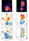 |
Fig. 2 GGD 27-MM2 molecular line emission from N2H+, CH3CN, and H2CO molecular lines. (a) Intensity map of the N2H+. (b) Intensity map of the CH3CN. (c) Velocity map of the N2H+. (d) Velocity map of CH3CN. (e) Velocity dispersion map of the N2H+. (f) Velocity dispersion map of the CH3CN. The H2CO molecular line emission is depicted in all panels as white (panels a and b) and black (panels c–f) contours; the contours levels are the same as in Fig. 1. The gray contours are the intensity map of the emission of N2H+ (panels cand e) and CH3CN (panels d and f); the contours levels start from 5σ and are in steps of 5σ, 10σ, 15σ, and 20σ, where σ = 30.3 mJy beam−1 km s−1 for the N2H+ emission, and start from 5σ with steps of 3σ, 6σ, 9σ, and 12σ, where σ = 6.8 mJy beam−1 km s−1, for the CH3CN emission. The synthesized beams are shown in the lower-left corners. In panels a and b, a green star marks the position of the source MC taken from Qiu & Zhang (2009), and yellow crosses marks the positions of the continuum sources reported by Busquet et al. (2019). Blue diamonds in panel bindicate the positions where we have extracted the spectra of the CH3CN. |
3.2 Morphology in the MM2(E) surroundings
To test that the molecular outflow is colliding with the MC cloudlet, we compared the outflow structure with the emission of N2H+ and CH3CN. Figures 2a and 2b present the intensity maps of N2H+ and CH3CN overlaid in white contours the emission of the H2CO, respectively. The maps are integrated over a velocity range of −0.05–21.95 km s−1 and 9.37–22.10 km s−1 for the N2H+ and CH3CN, respectively. The emission of the N2H+ traces the molecular cloud around the emission of the outflow, where protostars are forming, as indicated by the continuum emission of these sources (yellow crosses; Busquet et al. 2019). On the other hand, the CH3CN traces the emission around the central source MM2(E) and the MC cloudlet.
The emission of the N2H+ traces the projected area of ~8″ × 7″ (~11 200 × 9800). This area corresponds to the emission of NH3 previously reported by Gómez et al. (2003), where they found that it corresponds to the molecular cloud around the protostellar system GGD 27-MM2, with a gas temperature of ~150 K and a mass of H2 of 16 M⊙. It is noteworthy that the N2H+ has an internal cavity that spatially corresponds to the emission of the molecular outflow traced by H2CO; therefore, we can assume that the molecular outflow has swept up the material of the molecular gas.
As mentioned above, the emission of the CH3CN appears to be concentrated in the regions around the central source MM2(E) and MC. However, we detect a weaker emission of CH3CN between these regions and therefore can assume that the CH3CN also traces the inner part of the molecular outflow.
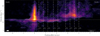 |
Fig. 3 PV diagram of the H2CO emission along the outflow axis. This orientation of the axis was estimated by joining the peak of the MM2(E) continuum emission and the position of the MC source. Dotted lines mark the position of the source (vertical) and the velocity of the system, Vsys ≃ 11.5 km s−1 (horizontal). Vertical dashed lines indicate the position where the perpendicular PV diagrams are made (see Fig. 4). The contour levels start at 2σ and are in steps of 2σ, 4σ, 6σ, and 8σ, where σ = 2.1 mJy beam−1. The white bar represents the angular resolution |
![Mathematical equation: $\[0^{\prime\prime}_\cdot18\]$](/articles/aa/full_html/2025/03/aa53196-24/aa53196-24-eq10.png)
3.3 Kinematics in the MM2(E) surroundings
Figures 2c and 2e show the ALMA first moment or intensity-weighted velocity map and the ALMA second moment or intensity-weighted velocity dispersion map of the emission of N2H+, respectively. These maps were integrated over a velocity range of −0.05–7.02 km s−1, corresponding to hyperfine line F1, F = 1, 0 → 1, 1 (e.g., Caselli et al. 1995; Álvarez-Gutiérrez et al. 2024). The difference in the integration range between the velocity maps and the intensity map arises because the N2H+ has seven hyperfine lines, of which only the first is not contaminated by the others.
It is noteworthy that the cloud exhibits a south-north velocity gradient of ~3 km s−1 and a line width of ~1.5 km s−1. While the velocity gradient may be associated with the expansion of an irregular cloud, the line width could be produced by turbulence of the gas at different spatial scales.
Figures 2d and 2f depict the velocity and velocity dispersion maps of the emission of CH3CN with the intensity maps of CH3CN and H2CO overlaid in gray and black contours, respectively. The velocity maps were integrated over a velocity range from 8.57–14.14 km s−1, corresponding to hyperfine line K=0 (e.g., Purcell et al. 2006). Similar to the emission of N2H+, the integration range differs from that of the intensity map because the CH3CN has four distinct transitions (see Sect. 2.1), of which three are blended.
CH3CN, like H2CO, traces the molecular outflow and thus exhibits the same south-north velocity gradient. Nevertheless, the velocity gradient associated with CH3CN is on the order of ~3 km s−1, and the velocity gradient associated with H2CO is ~7 km s−1. Additionally, the velocity dispersion map presents a line width of ~1.5 km s−1, which could be associated with the material being dragged or with shocks between the outflow and the cavity walls.
The emission of the H2CO and CH3CN traces the molecular outflow associated with MM2(E) inside the cavity detected in the N2H+ cloud. The two molecules show similar kinematic features, and the outflow extends up to ~4″, where it appears to be colliding with MC. In the following sections, we focus on the shocked region associated with the MC cloudlet.
3.4 Shocked region and molecular outflow
Figure 3 shows a position–velocity (PV) diagram of H2CO emission created from a cut taken along the outflow axis (dashed black line in Fig. 1b). The strongest emission presents a large velocity dispersion at the position of the protostellar disk/envelope (zero positional offset), which may be due to gas rotation around the protostar(s). The extended emission observed around the MM2(E) systemic velocity ~11.5 km s−1 is associated with the molecular cloud or envelope mainly surrounding the lower half (up to ~3″) of the outflow from MM2(E). A strong shock reaching radial velocities over 22 km s−1 is present at ~![Mathematical equation: $\[3^{\prime\prime}_\cdot6\]$](/articles/aa/full_html/2025/03/aa53196-24/aa53196-24-eq11.png) . However, the high-velocity shocked gas extends from
. However, the high-velocity shocked gas extends from ![Mathematical equation: $\[2^{\prime\prime}_\cdot8\]$](/articles/aa/full_html/2025/03/aa53196-24/aa53196-24-eq12.png) to
to ![Mathematical equation: $\[5^{\prime\prime}_\cdot1\]$](/articles/aa/full_html/2025/03/aa53196-24/aa53196-24-eq13.png) from the protostar. In general, we note that the PV diagram does not present the characteristic parabolic shape expected for a wide-angle disk wind (Lee et al. 2000), but a convex spur-like structure, similar to the shape expected for a jet-driven outflow inclined with respect to the plane of the sky (see, e.g., Fig. 5 of Lee et al. 2001).
from the protostar. In general, we note that the PV diagram does not present the characteristic parabolic shape expected for a wide-angle disk wind (Lee et al. 2000), but a convex spur-like structure, similar to the shape expected for a jet-driven outflow inclined with respect to the plane of the sky (see, e.g., Fig. 5 of Lee et al. 2001).
The vertical dashed lines (C1–C9) in Fig. 3 indicate the positional offsets used to generate a series of PV diagrams perpendicular to the outflow axis (Fig. 4). Analyzing these cuts in detail, we find that in the region closer to the MM2(E) disk/envelope (panels C1–C3), the PV diagrams trace the emission associated with the cavity walls of the molecular outflow. The walls are identified as almost vertical finger-like structures with large spreads in velocity (similar to shocks) or elongated blobs at high velocities. In particular, panel C1 presents an unresolved structure with a high-velocity dispersion (dashed green line); this spatially unresolved structure could be regarded as material directly ejected from the disk and/or as the outflow cavity walls (formed as a result of the interaction between the outflow and the ambient medium; Lee et al. 2000). Panel C2 shows the emission of the cavity walls of the molecular outflow (external dashed lines), these walls appear as elongated fingers with a high velocity dispersion (~6 km s−1). The unresolved emission region between the external cavity walls observed in panel C2 could be associated with an internal layer of the molecular outflow, which has been previously detected in several sources, such as HH 46/47 (Zhang et al. 2019), DO Tauri (Fernández-López et al. 2020), DG Tau B (de Valon et al. 2020, 2022), and HH 30 (López-Vázquez et al. 2024). This internal layer is confirmed in panel C3, where the emission of the four elongated fingers with similar velocity dispersion (~9 km s−1) is observed. In this panel, we interpret the cavity walls as being traced by the external fingers (external dashed lines), located at approximately ±1″ of the outflow axis, while the internal layer is associated with the internal fingers (internal dashed lines), located atapproximately ±0.6″ from the outflow axis.
In the central region (panels C4–C5), the H2CO emission traces two different finger-like structures associated with the cavity walls. This same pattern has been observed in other sources where the inclination angle with respect to the plane of the sky is i ≥ 30° such as HH 46/47 (Zhang et al. 2019) and DG Tau B (de Valon et al. 2020, 2022). The H2CO is also tracing the extended cloud emission comprising all the sources in this region (see channels from 10.0 to 11.5 km s−1 and Fernández-López et al. 2011b), which indicates that the observed emission from the walls probably comes from gas dragged by the outflow. A distinct aspect, evident also from the moment 0 map (Fig. 1), is that it has a brighter eastern side in H2CO. This feature, along with the characteristic shape of MM2(E)’s molecular outflow, could be associated with the presence of a very asymmetric jet such as L1157 (Podio et al. 2016), or with two or more episodic ejections of material as observed in IRAS 21078+5211 (Moscadelli et al. 2022, 2023). An alternative explanation is that the density spatial distribution of the surrounding material is not homogeneous, which may cause differences in the excitation of molecules and produce asymmetries in the outflow shape emission.
In regions far away from the central source (panels C6–C9), the velocity cuts mainly show the formation of a strong shock and the downstream perturbations of the gas produced by the putative collision between the outflow and the MC cloudlet. Panels C6 and C7 show the behavior of the gas just upstream the MC position (C8; the dashed line in Fig. 3). Both panels show the walls of the molecular outflow, and possibly the molecular jet impacting dense gas at a more redshifted velocity than the systemic velocity (≈13–14 km s−1) and creating a shock. The horizontal structures observed in panel C6 at ~11.5 km s−1 and ~14 km s−1 could be associated with the remnant cloud system velocity of the MM2(E) and with the MC cloudlet, respectively. Panel C9 traces shocked material in a more turbulent and spray-like way. The measured outflow width downstream MC is larger (~![Mathematical equation: $\[1^{\prime\prime}_\cdot0\]$](/articles/aa/full_html/2025/03/aa53196-24/aa53196-24-eq15.png) ) than the outflow region from the main body (between
) than the outflow region from the main body (between ![Mathematical equation: $\[1^{\prime\prime}_\cdot7\]$](/articles/aa/full_html/2025/03/aa53196-24/aa53196-24-eq16.png) and
and ![Mathematical equation: $\[2^{\prime\prime}_\cdot8\]$](/articles/aa/full_html/2025/03/aa53196-24/aa53196-24-eq17.png) ; panels C4-C6), which is ~
; panels C4-C6), which is ~![Mathematical equation: $\[0^{\prime\prime}_\cdot6\]$](/articles/aa/full_html/2025/03/aa53196-24/aa53196-24-eq18.png) . This width increase also suggests and supports the scenario of an upstream pounding of the outflow with a dense cloudlet (Raga et al. 2002).
. This width increase also suggests and supports the scenario of an upstream pounding of the outflow with a dense cloudlet (Raga et al. 2002).
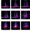 |
Fig. 4 PV diagrams perpendicular to the outflow axis of the H2CO emission at the different heights indicated by vertical dashed lines in Fig. 3. Dotted white lines mark the position of the outflow axis (vertical) and the systemic velocity at 11.5 km s−1 (horizontal). Dashed green lines in all panels trace the putative structures associated with the outflow cavity walls and shocked gas. The contour levels start at 2σ and are in steps of 2σ, 4σ, 6σ, and 8σ, where σ = 2.1 mJy beam−1. The white bar represents the angular resolution ( |
![Mathematical equation: $\[0^{\prime\prime}_\cdot18\]$](/articles/aa/full_html/2025/03/aa53196-24/aa53196-24-eq14.png)
4 Analysis and discussion
4.1 Outflow mass and energy
We estimated the column density of the outflow gas using the expressions from Mangum & Shirley (2015) adapted to the H2CO (41,3−31,2) line emission. The H2CO (41,3−31,2) line emission considered (with an intensity over 3 − σ) is generally optically thin through MM2(E)’s outflow, so we used the simplified expression of Eq. (86) in Mangum & Shirley (2015). As a proxy for the excitation temperature, we utilized a range of values between 30 and 70 K derived in the analysis of the CH3CN K-ladder emission (see Sect. 4.2). From this, we also derived the mass, momentum, and kinetic energy of the outflow following a procedure analogous to that in, for example, Vazzano et al. (2021) (note that we give the momentum and energy without correcting by the unknown outflow inclination with respect to the line of sight). We adopted an H2CO abundance with respect to H2 of 10−10 (Gerner et al. 2014; Tang et al. 2018; Gieser et al. 2021; Zhao et al. 2024), which produces an outflow mass between 1.7 M⊙ and 2.1 M⊙. Likewise, the derived momentum, Pout flow, and kinetic energy, Eout flow, ranges are 7.8–10.1 M⊙ km s−1 and 5.0–6.6×1044 erg, respectively.
The size of the molecular outflow is z ≃ ![Mathematical equation: $\[4^{\prime\prime}_\cdot8\]$](/articles/aa/full_html/2025/03/aa53196-24/aa53196-24-eq19.png) ≃ 6720 au, and its outward velocity is Vz ≃ 9 km s−1 (this velocity is the difference between the maximum observed velocity in channel maps in Fig. A.2, ~21 km s−1, and the systemic velocity, ~11.5km s−1). From this, we obtain the dynamical time τdyn = z/Vz ≃ 3500 yr. We estimate a mass-loss outflow rate of
≃ 6720 au, and its outward velocity is Vz ≃ 9 km s−1 (this velocity is the difference between the maximum observed velocity in channel maps in Fig. A.2, ~21 km s−1, and the systemic velocity, ~11.5km s−1). From this, we obtain the dynamical time τdyn = z/Vz ≃ 3500 yr. We estimate a mass-loss outflow rate of ![Mathematical equation: $\[\dot{M}_{out flow}\]$](/articles/aa/full_html/2025/03/aa53196-24/aa53196-24-eq20.png) = 4.9–6.0×10⁻⁴ M⊙ yr−1. These values are consistent with the previously reported of outflows driven by massive stars (e.g., López-Sepulcre et al. 2009; Sánchez-Monge et al. 2013; Maud et al. 2015).
= 4.9–6.0×10⁻⁴ M⊙ yr−1. These values are consistent with the previously reported of outflows driven by massive stars (e.g., López-Sepulcre et al. 2009; Sánchez-Monge et al. 2013; Maud et al. 2015).
We next derived the mass of the dense gas clump, part of the parental molecular cloud enveloping the outflow from MM2(E). For this we used the HfS fitting tool on the hyperfine structure of the N2H+ (1–0) transition (Estalella 2017, panel a in Fig. 2). We estimate the average opacity of the main hyperfine line is about 0.3±0.1, which was taken into account to estimate the column density using the spectrum extracted over an area of 73 square arcseconds, limited by the 10σ contour in the integrated intensity map (velocity interval used: 9.9–15.3 km s−1; see panel c in Fig. 2), and the optically thin approximation (Eqs. (80) and (86) in Mangum & Shirley 2015). We also find an excitation temperature of 23±4 K, which agrees well with the value measured by Gómez et al. (2003) for the ammonia temperature of the emission associated with this clump. We found a value for the partition function Qrot by interpolating the values tabulated by the Cologne Database for Molecular Spectroscopy1 with a power law of the form Qrot(T) ≈ 3.88T1.02, which nicely fits the data between 9 and 500 K. The N2H+ column density is 1.4×1014 cm−2, and adopting an N2H+ abundance ranging between 1 and 2×10⁻¹⁰ (Shirley et al. 2005; Álvarez-Gutiérrez et al. 2024), we derive a hydrogen column density of 7.1–14.2×1023 cm−2. The total mass of the whole clump of gas is therefore 13.3–26.5 M⊙, a factor of 8–12 higher than the gas moved by the redshifted lobe of MM2(E)’s outflow. This mass is, again, consistent with that estimated by Gómez et al. (2003).
With all of this we can address now the potential of the outflow from MM2(E) to introduce and maintain turbulence in its surroundings and whether the outflow can potentially over-come the cloud’s gravity and disperse the gas. Following an analogous pathway as Plunkett et al. (2015) based on the outflow-regulated star formation model by Nakamura & Li (2014), we first estimated the turbulent energy as ![Mathematical equation: $\[E_{turb}=\frac{1}{2} M_{c l} \sigma_{3 D}^{2}\]$](/articles/aa/full_html/2025/03/aa53196-24/aa53196-24-eq21.png) , with σ3D = (3/8ln(2))0.5Δvturb. From the N2H+ emission, we estimate that the dense part of the cloud surrounding MM2(E) has an approximate radius of 5″ (~7000 au), and a σ3D = 1.49km s−1, estimated by using Δvturb = Δvobserved − Δvthermal. The turbulent energy is 2.9–5.9 × 1044 erg, comparable to MM2(E)’s outflow energy. In addition, would the cloud be spherical, its free-fall time is 2.0–2.8×10⁴ yr (for Mcl values 13.3–26.5M⊙). Hence, the free-fall time tf f is about a factor of 8 larger than the outflow dynamical time (we estimate tdyn ≃ 3500 yr for the outflow of MM2(E), although without correcting for its inclination). From tf f we can derive the momentum dissipation time, tdiss = tf f · 3.9 κ/Mrms ≃ 1.7 × 10⁴ yr, using that the parameter κ ~ 1 (turbulence driving length approximately matches the Jean’s length) and estimating the Mach number as
, with σ3D = (3/8ln(2))0.5Δvturb. From the N2H+ emission, we estimate that the dense part of the cloud surrounding MM2(E) has an approximate radius of 5″ (~7000 au), and a σ3D = 1.49km s−1, estimated by using Δvturb = Δvobserved − Δvthermal. The turbulent energy is 2.9–5.9 × 1044 erg, comparable to MM2(E)’s outflow energy. In addition, would the cloud be spherical, its free-fall time is 2.0–2.8×10⁴ yr (for Mcl values 13.3–26.5M⊙). Hence, the free-fall time tf f is about a factor of 8 larger than the outflow dynamical time (we estimate tdyn ≃ 3500 yr for the outflow of MM2(E), although without correcting for its inclination). From tf f we can derive the momentum dissipation time, tdiss = tf f · 3.9 κ/Mrms ≃ 1.7 × 10⁴ yr, using that the parameter κ ~ 1 (turbulence driving length approximately matches the Jean’s length) and estimating the Mach number as ![Mathematical equation: $\[M_{r m s}=\sigma_{3 D} \cdot \sqrt{2.72 ~m_{H} /\left(K_{B} ~T\right)} \simeq 5.6\]$](/articles/aa/full_html/2025/03/aa53196-24/aa53196-24-eq22.png) . Therefore, the momentum rate of the outflow (
. Therefore, the momentum rate of the outflow (![Mathematical equation: $\[\dot{P}_{out ~flow}=P_{out~flow} / \tau_{dyn} \approx 1.4-1.8 \times 10^{28} ~\mathrm{erg} ~\mathrm{cm}^{-1}\]$](/articles/aa/full_html/2025/03/aa53196-24/aa53196-24-eq23.png) ) is about 7–9 times larger than the momentum dissipation rate of the internal turbulent motion in the cloud (
) is about 7–9 times larger than the momentum dissipation rate of the internal turbulent motion in the cloud (![Mathematical equation: $\[\dot{P}_{c l}= -0.21 M_{c l} \sigma_{3 D} / t_{diss} \approx-2 \times 10^{27} ~\mathrm{erg} ~\mathrm{cm}^{-1}\]$](/articles/aa/full_html/2025/03/aa53196-24/aa53196-24-eq24.png) ; see Nakamura & Li 2014), and it is plausible that the studied outflow is entering and replenishing a significant amount of turbulence in its parental cloud at spatial scales smaller than its approximate length (~7″), since it completely crosses its most dense part.
; see Nakamura & Li 2014), and it is plausible that the studied outflow is entering and replenishing a significant amount of turbulence in its parental cloud at spatial scales smaller than its approximate length (~7″), since it completely crosses its most dense part.
To compare the outflow energy and the gravitational binding of the cloud W, we used the expression ![Mathematical equation: $\[W=-G M_{c l}^{2} / R_{c l}\]$](/articles/aa/full_html/2025/03/aa53196-24/aa53196-24-eq25.png) , where G is the gravitational constant, Mcl is the mass of the cloud, and Rcl is the radius of the cloud. In this case, W ranges from −5.0 × 1044 erg to −1.8 × 1045 erg (again depending on the mass of the cloud). Nakamura & Li (2014) defined the nondimensional parameter ηout = −2Eout flow/W to compare the cloud and the outflow energies. For MM2(E), ηout ranges between 0.55 and 2.64. These relatively high values of ηout indicate that MM2(E)’s outflow is very powerful, can disrupt/unbind large amounts of gas, and has the ability to erode large parts of its natal cloud. It has the potential to destroy or tremendously perturb smaller scale cores, such as ALMA 12’s or the MC, directly impacting sites of ongoing star-formation. Even if we have underestimated the abundance of H2CO (which may result in a lower outflow mass and energy), and it is larger by a factor of 5, ηout would still be close to 1, demonstrating the high power of this outflow.
, where G is the gravitational constant, Mcl is the mass of the cloud, and Rcl is the radius of the cloud. In this case, W ranges from −5.0 × 1044 erg to −1.8 × 1045 erg (again depending on the mass of the cloud). Nakamura & Li (2014) defined the nondimensional parameter ηout = −2Eout flow/W to compare the cloud and the outflow energies. For MM2(E), ηout ranges between 0.55 and 2.64. These relatively high values of ηout indicate that MM2(E)’s outflow is very powerful, can disrupt/unbind large amounts of gas, and has the ability to erode large parts of its natal cloud. It has the potential to destroy or tremendously perturb smaller scale cores, such as ALMA 12’s or the MC, directly impacting sites of ongoing star-formation. Even if we have underestimated the abundance of H2CO (which may result in a lower outflow mass and energy), and it is larger by a factor of 5, ηout would still be close to 1, demonstrating the high power of this outflow.
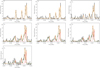 |
Fig. 5 Extracted spectra of the CH3CN (5–4) K-ladder from the areas marked with blue dots in panel b of Fig. 2. The labels S 1 to S 7 indicate the location of the points, with S1 being the point over the MM2(E) and S7 the most distant point in the south-north direction. The black line represents the data obtained from the observations, and the orange line shows the best fit. For panels S1 to S3 we used only one velocity component for our fit, whereas for panels S4 to S7 we used two additional velocity components (green and red lines). |
4.2 The shock at the position of the MC core
Figure 2 shows a deep N2H+ cavity (panel a) and a CH3CN emission enhancement toward the MC location (panel b). This spatial anticorrelation between N2H+ and CH3CN emissions closely follows the MM2(E) outflow path. The CH3CN emission could be enhanced by the shocks of the outflow revealed by Figs. 3 and 4. At the same time, the physical conditions of the post-shocked gas may destroy the N2H+ from the quiescent gas of the molecular cloud (the molecule is easily destroyed by CO released from the grain mantles when gas temperature increases over 20 K; Jørgensen et al. 2004), which may also be dragged and dispersed by the outflow. A decrease on the abundance of N2H+ has also been seen in shocks associated with other outflows (Tobin et al. 2012; Podio et al. 2014). Moreover, the same anticorrelation between N2H+ and CH3CN is seen at the position of MM2(E), where an increase in temperature and the presence of multiple outflows could be causing it.
The CH3CN emission is seen at the location of MM2(E) and toward the northern lobe of its outflow, but it is specially enhanced in the area surrounding the MC position (about 4000 au×3000 au in size). To check the physical conditions of the outflow gas we extracted the spectra of the CH3CN (5–4) K–ladder from several locations along its main path (blue dots panel b in Fig. 2). At every position we fitted synthetic spectra derived by solving the radiative transfer equation for an isothermal object in local thermodynamic equilibrium (following a procedure analogous to, e.g., that in Möller et al. 2017), using one or two independent layers when the spectra showed one or two kinematic components, respectively. The fitting was performed with a Python code that uses a nonlinear least-squares minimization algorithm to search for the best fit of the observed data (Newville et al. 2020). The results from the fits are presented in Fig. 5. In addition, Fig. 6 presents a summary of the fitted parameters as a function of distance to the MM2(E) protostar. At any distance from the position of MM2(E), the CH3CN shows supersonic line widths (>2.4 km s−1), with excitation temperatures over ≈40 K. At distances from MM2(E) larger than ~2″ two-velocity components (red and green lines in panels S4–S7 of Fig. 5) are included in the fitting. Incorporating these components into positions S4 through S7 improves the model and reduces the residuals. An inspection of Fig. 6 shows a line component with a velocity between 11.0 and 13.5 km s−1 (orange squares in panel (d); see also the overall south-north velocity gradient in various gas tracers in Figs. 2, A.1, and A.2), persistent beyond the 2″. The gas traced by this component is warm (40–50 K), with mild line-widths (2–4 km s−1), and a stable column density of about 2 × 1013 cm−2. At distances from MM2(E) larger than 2″ there is a second high-velocity component (at >18 km s−1), with warmer (Tex ranges 55–120 K) and higher density gas (~1014 cm−2). This component is probably related with strong redshifted shocks (ΔV ≈ 8 km s−1).
While the two kinematic CH3CN components are likely due to shocks, the colder and less dense component seems to trace supersonic but mild shocks, maybe associated with the outflow cavity expansion against the parental cloud (seen in N2H+ and NH3; Gómez et al. 2003), and the warm and dense component could be linked to a more extreme interaction. Two alternatives could potentially explain the latter: (1) A collision between the outflow and a dense pocket of gas or cloudlet (e.g., Raga et al. 1998; Hartigan 2003), or (2) the outflow is escaping the rear part of the molecular cloud, producing strong shocks (see analogous cases in HH 80–81, HH46/47, and IRAS 16059-3857 Heathcote et al. 1998; Arce et al. 2013; Vazzano et al. 2021). On one hand, the MC (and possibly ALMA 12 as well) position matches with shocked gas profiles (large line-widths and spectral wings with high redshifted velocity; Fig. 1; see also Fernández-López et al. 2011b). This is due to the impinging fast wind, which is ablating portions of the MC dense cloudlet (which was initially at a slightly redshifted radial velocity than MM2(E)).
On the other hand, the point at which the flow starts showing the two spectral components and the strong shock profiles coincides with an overall decrease in the N2H+ abundance that may be tracing the northern edge of the denser part of the molecular cloud. This morphology suggests that fast, very hot bullets may expand violently as they escape from the cloud into a low pressure and hot surrounding, such as in HH 80A and HH 81A (Heathcote et al. 1998). In addition, the H2CO flow emission does not extend farther north, although there is evidence that the associated jet does (Bally & Reipurth 2023).
Another piece of evidence that supports the presence of these extreme shocks is the H2CO X-shape at the location of the old MC source (green star in Figs. 1 and A.1). North of the crossing point at MC, the gas appears more turbulent, less ordered (see Fig. 4), as expected after a collision of a fast wind an a dense cloudlet partially ablated (see the bottom panel in Fig. 2 of Raga et al. 1998).
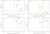 |
Fig. 6 Physical conditions of the gas of the emission of CH3CN associated with the GGD 27-MM2(E) molecular outflow as a function of the distance to the central source. (a) Excitation temperature. (b) Column density. (c) Line width. (d) Velocity of the gas. Error bars are derived from the model (see the main text for more details). Orange and green squares show results from a simultaneous fitting of two kinematic components. The orange squares are probably associated with weak/mild shocks from the expanding outflow walls, whereas the green squares are possibly linked with a more violent shock between the fast wind and a dense cloudlet (MC source), whose position is marked by a dashed vertical line at about |
![Mathematical equation: $\[3^{\prime\prime}_\cdot5\]$](/articles/aa/full_html/2025/03/aa53196-24/aa53196-24-eq26.png)
4.3 Several outflow ejections?
In the region close to the central source, z ≤ ![Mathematical equation: $\[1^{\prime\prime}_\cdot2\]$](/articles/aa/full_html/2025/03/aa53196-24/aa53196-24-eq27.png) , the PV diagrams depicted in Fig. 4 show (particularly in panel C3) that the emission of the H2CO is dominated by two distinct layers: an external layer at a distance of approximately ±1″ from the outflow axis and an internal layer located at approximately ±
, the PV diagrams depicted in Fig. 4 show (particularly in panel C3) that the emission of the H2CO is dominated by two distinct layers: an external layer at a distance of approximately ±1″ from the outflow axis and an internal layer located at approximately ±![Mathematical equation: $\[0^{\prime\prime}_\cdot6\]$](/articles/aa/full_html/2025/03/aa53196-24/aa53196-24-eq28.png) . These layers are also observed in the emission above 3σ in the channel maps of Fig. A.2, particularly in the velocity range of ~12.5–16 km s−1. The multilayer structure has been observed in several sources, such as HH 46/47 (Zhang et al 2019), DO Tauri (Fernández-López et al. 2020), DG Tau B (de Valon et al. 2020, 2022), and HH 30 (López-Vázquez et al 2024), where the authors suggested that the multiple layers are associated with episodic ejections of the material from the accretion disk. Assuming that the two layers correspond to different ejections, the outer layer could represent an older ejection, while the internal layer is related to a younger ejection. This implies that the material from the younger ejection has not traveled for a long time and is therefore not detected at heights z >
. These layers are also observed in the emission above 3σ in the channel maps of Fig. A.2, particularly in the velocity range of ~12.5–16 km s−1. The multilayer structure has been observed in several sources, such as HH 46/47 (Zhang et al 2019), DO Tauri (Fernández-López et al. 2020), DG Tau B (de Valon et al. 2020, 2022), and HH 30 (López-Vázquez et al 2024), where the authors suggested that the multiple layers are associated with episodic ejections of the material from the accretion disk. Assuming that the two layers correspond to different ejections, the outer layer could represent an older ejection, while the internal layer is related to a younger ejection. This implies that the material from the younger ejection has not traveled for a long time and is therefore not detected at heights z > ![Mathematical equation: $\[1^{\prime\prime}_\cdot2\]$](/articles/aa/full_html/2025/03/aa53196-24/aa53196-24-eq29.png) .
.
Another possible explanation for the shape observed in panels C1–C3 of Fig. 4 and in the channel maps of Fig. A.1 is that the H2CO emission is tracing multiple streamlines created by the presence of overdensities launched from the accretion rotating disk with an inclination from the polar direction (e.g. IRAS 21078+5211 Moscadelli et al. 2023). However, given that our observations do not have enough spatial resolution and sensitivity to resolve and trace the full path of all the possible streamlines, we cannot confirm this scenario.
5 Conclusions
We have presented a detailed analysis of ALMA observations of the molecular line emissions of the H2CO, CH3CN, and N2H+ from the molecular outflow, as well as the emission of the N2H+ from the molecular cloud, both associated with the protostellar system GGD 27-MM2(E). Our main results are as follows.
The emission of N2H+ traces a molecular cloud surrounding GGD27 MM2(E) and MM2(W) (ALMA 17 and ALMA 13, respectively). Other continuum sources, such as ALMA 6, ALMA 12, and ALMA 18, are located within the cloud. The N2H+ cloud exhibits an internal cavity that spatially corresponds to the emission of the molecular outflow traced by H2CO. We estimate that the mass of the envelope is between 13.3 and 26.5 M⊙; this value is consistent with those reported by Gómez et al. (2003).
The molecular outflow within the cloud is depicted by the emission of H2CO and CH3CN. While the H2CO is associated with the material dragged from the cloud and traces the walls of the outflow, the emission of CH3CN is concentrated around the central sources MM2(E) and MM2(W), as well as in the vicinity of the MC. This distribution could indicate that the outflow is colliding with the MC.
Through the emission of H2CO, we estimate that the outflow has a mass of 1.7–2.1 M⊙, a momentum of 7.8–10.1 M⊙ km s−1, and a kinetic energy of 5.0–6.6×1044 erg, values consistent with outflows driven by massive stars. On the other hand, the mass-loss rate of the outflow is 4.9–6.0×10⁻⁴ M⊙ yr−1, consistent with the values reported in the literature.
We quantified the turbulence and gravity energies and find that the outflow contributes a significant amount of turbulence to its parent cloud. The outflow is very powerful and has the ability to erode large parts of its parent cloud. It also has the potential to destroy or perturb smaller cores, such as ALMA 12 and MC.
The X-shaped feature detected to the north of the H2CO molecular outflow suggests that this outflow is colliding with the MC cloudlet. This conclusion is supported by the emission of CH3CN, where we observe an increase in the excitation temperature, column density, line width, and velocity of the gas in the region around the MC. These increases are associated with the perturbation of the gas due to the shock. The perturbation is also evident in the PV diagrams of the H2CO emission, where we detect spray-shocked material downstream of the MC position with a larger width than the main outflow body.
Acknowledgements
We thank an anonymous referee for very useful suggestions that improved the presentation of this paper. We are indebted to Pablo Fonfría for his fruitful discussions and advices. J.A.L.V. and C.F.L. acknowledge grants from the National Science and Technology Council of Taiwan (NSTC 112–2112–M–001–039–MY3). M.F.L. acknowledges support from the European Research Executive Agency HORIZON-MSCA-2021-SE-01 Research and Innovation programme under the Marie Skłodowska-Curie grant agreement number 101086388 (LACEGAL). M.F.L. also acknowledges the warmth and hospitality of the ICE-UB group of star formation. S.C. acknowledges financial support from UNAM-PAPIIT IN107324, and CONACyT CF-2023-I-232 grants, México. J.M.G. and G.B. acknowledge support from the PID2020-117710GB-I00 and PID2023-146675NB-I00 grants funded by MCIN/ AEI /10.13039/501100011033. L.A.Z. acknowledges financial support from CONACyT-280775 and UNAM-PAPIIT IN110618, and IN112323 grants, México. R.G.M. acknowledges support from UNAM-PAPIIT project IN108822. This paper makes use of the following ALMA data: ADS/JAO.ALMA#2015.1.00480.S. ALMA is a partnership of ESO (representing its member states), NSF (USA) and NINS (Japan), together with NRC (Canada), NSTC and ASIAA (Taiwan), and KASI (Republic of Korea), in cooperation with the Republic of Chile. The Joint ALMA Observatory is operated by ESO, AUI/NRAO and NAOJ.
Appendix A Channel maps
Figures A.1 and A.2 show the complete velocity cube of the emission of the H2CO molecular line with a channel width of 0.5 km s−1. The arrows in both figures represent the direction of the CO molecular outflow, the redshifted northeast and northwest (red arrows) and blueshifted southeast (blue arrow).
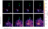 |
Fig. A.1 Blueshifted channel maps of the H2CO molecular line emission of the GGD 27–MM2(E) protostellar system. The channel velocity in km s−1 is indicated in the top-left corner. The contours start at 3σ and are in steps of 3σ, 6σ, 9σ, and 12σ, where σ = 2.1 mJy beam−1. The cyan dot and square mark the position of the CH3OH and H2O maser sources obtained from Kurtz et al. (2004) and Kurtz & Hofner (2005), respectively. The green star marks the position of the source MC taken from Qiu & Zhang (2009). The synthesized beam in all panels is shown in the lower-left corner. The two red arrows present the redshifted NE and NW CO outflow directions, and the blue arrow is the blueshifted SE CO outflow direction taken from Fernández-López et al. (2013). |
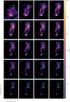 |
Fig. A.2 Same as Fig. A.1 but for the redshifted channel maps. |
References
- Añez-López, N., Osorio, M., Busquet, G., et al. 2020, ApJ, 888, 41 [CrossRef] [Google Scholar]
- Álvarez-Gutiérrez, R. H., Stutz, A. M., Sandoval-Garrido, N., et al. 2024, A&A, 689, A74 [NASA ADS] [CrossRef] [EDP Sciences] [Google Scholar]
- Anglada, G., López, R., Estalella, R., et al. 2007, AJ, 133, 2799 [Google Scholar]
- Arce, H. G., Mardones, D., Corder, S. A., et al. 2013, ApJ, 774, 39 [CrossRef] [Google Scholar]
- Bachiller, R. 1996, ARA&A, 34, 111 [NASA ADS] [CrossRef] [Google Scholar]
- Bally, J. 2016, ARA&A, 54, 491 [Google Scholar]
- Bally, J., & Reipurth, B. 2023, ApJ, 958, 99 [NASA ADS] [CrossRef] [Google Scholar]
- Beltrán, M. T., Girart, J. M., Estalella, R., Ho, P. T. P., & Palau, A. 2002, ApJ, 573, 246 [CrossRef] [Google Scholar]
- Blandford, R. D., & Payne, D. G. 1982, MNRAS, 199, 883 [CrossRef] [Google Scholar]
- Busquet, G., Girart, J. M., Estalella, R., et al. 2019, A&A, 623, L8 [NASA ADS] [CrossRef] [EDP Sciences] [Google Scholar]
- Carrasco-González, C., Galván-Madrid, R., Anglada, G., et al. 2012, ApJ, 752, L29 [Google Scholar]
- CASA Team (Bean, B., et al.) 2022, PASP, 134, 114501 [NASA ADS] [CrossRef] [Google Scholar]
- Caselli, P., Myers, P. C., & Thaddeus, P. 1995, ApJ, 455, L77 [Google Scholar]
- Cunningham, N. J., Moeckel, N., & Bally, J. 2009, ApJ, 692, 943 [NASA ADS] [CrossRef] [Google Scholar]
- de Valon, A., Dougados, C., Cabrit, S., et al. 2020, A&A, 634, L12 [NASA ADS] [CrossRef] [EDP Sciences] [Google Scholar]
- de Valon, A., Dougados, C., Cabrit, S., et al. 2022, A&A, 668, A78 [NASA ADS] [CrossRef] [EDP Sciences] [Google Scholar]
- Estalella, R. 2017, PASP, 129, 025003 [NASA ADS] [CrossRef] [Google Scholar]
- Fernández-López, M., Curiel, S., Girart, J. M., et al. 2011a, AJ, 141, 72 [CrossRef] [Google Scholar]
- Fernández-López, M., Girart, J. M., Curiel, S., et al. 2011b, AJ, 142, 97 [CrossRef] [Google Scholar]
- Fernández-López, M., Girart, J. M., Curiel, S., et al. 2013, ApJ, 778, 72 [CrossRef] [Google Scholar]
- Fernández-López, M., Zapata, L. A., Rodríguez, L. F., et al. 2020, AJ, 159, 171 [Google Scholar]
- Fernández-López, M., Girart, J. M., López-Vázquez, J. A., et al. 2023, ApJ, 956, 82 [CrossRef] [Google Scholar]
- Gerner, T., Beuther, H., Semenov, D., et al. 2014, A&A, 563, A97 [NASA ADS] [CrossRef] [EDP Sciences] [Google Scholar]
- Gieser, C., Beuther, H., Semenov, D., et al. 2021, A&A, 648, A66 [EDP Sciences] [Google Scholar]
- Girart, J. M., Fernández-López, M., Li, Z. Y., et al. 2018, ApJ, 856, L27 [CrossRef] [Google Scholar]
- Gómez, Y., Rodríguez, L. F., Girart, J. M., Garay, G., & Martí, J. 2003, ApJ, 597, 414 [Google Scholar]
- Hartigan, P. 2003, Ap&SS, 287, 111 [NASA ADS] [Google Scholar]
- Hartigan, P., Raymond, J., & Hartmann, L. 1987, ApJ, 316, 323 [Google Scholar]
- Hartigan, P., Bally, J., Reipurth, B., & Morse, J. A. 2000, in Protostars and Planets IV, eds. V. Mannings, A. P. Boss, & S. S. Russell (Tucson: University of Arizona Press), 841 [Google Scholar]
- Heathcote, S., Reipurth, B., & Raga, A. C. 1998, AJ, 116, 1940 [Google Scholar]
- Jørgensen, J. K., Hogerheijde, M. R., van Dishoeck, E. F., Blake, G. A., & Schöier, F. L. 2004, A&A, 413, 993 [NASA ADS] [CrossRef] [EDP Sciences] [Google Scholar]
- Kajdič, P., Reipurth, B., Raga, A. C., Bally, J., & Walawender, J. 2012, AJ, 143, 106 [Google Scholar]
- Kurtz, S., & Hofner, P. 2005, AJ, 130, 711 [NASA ADS] [Google Scholar]
- Kurtz, S., Hofner, P., & Álvarez, C. V. 2004, ApJS, 155, 149 [Google Scholar]
- Kwon, W., Fernández-López, M., Stephens, I. W., & Looney, L. W. 2015, ApJ, 814, 43 [NASA ADS] [CrossRef] [Google Scholar]
- Lee, C.-F., Mundy, L. G., Reipurth, B., Ostriker, E. C., & Stone, J. M. 2000, ApJ, 542, 925 [NASA ADS] [CrossRef] [Google Scholar]
- Lee, C.-F., Stone, J. M., Ostriker, E. C., & Mundy, L. G. 2001, ApJ, 557, 429 [NASA ADS] [CrossRef] [Google Scholar]
- López-Sepulcre, A., Codella, C., Cesaroni, R., Marcelino, N., & Walmsley, C. M. 2009, A&A, 499, 811 [NASA ADS] [CrossRef] [EDP Sciences] [Google Scholar]
- López, R., Estalella, R., Beltrán, M. T., et al. 2022, A&A, 661, A106 [NASA ADS] [CrossRef] [EDP Sciences] [Google Scholar]
- López-Vázquez, J. A., Lee, C.-F., Fernández-López, M., et al. 2024, ApJ, 962, 28 [CrossRef] [Google Scholar]
- Mangum, J. G., & Shirley, Y. L. 2015, PASP, 127, 266 [Google Scholar]
- Marti, J., Rodriguez, L. F., & Reipurth, B. 1993, ApJ, 416, 208 [Google Scholar]
- Martí, J., Rodríguez, L. F., & Torrelles, J. M. 1999, A&A, 345, L5 [NASA ADS] [Google Scholar]
- Masqué, J. M., Girart, J. M., Estalella, R., Rodríguez, L. F., & Beltrán, M. T. 2012, ApJ, 758, L10 [Google Scholar]
- Masqué, J. M., Rodríguez, L. F., Araudo, A., et al. 2015, ApJ, 814, 44 [CrossRef] [Google Scholar]
- Maud, L. T., Moore, T. J. T., Lumsden, S. L., et al. 2015, MNRAS, 453, 645 [Google Scholar]
- Maureira, M. J., Arce, H. G., Dunham, M. M., et al. 2017, ApJ, 838, 60 [NASA ADS] [CrossRef] [Google Scholar]
- Möller, T., Endres, C., & Schilke, P. 2017, A&A, 598, A7 [NASA ADS] [CrossRef] [EDP Sciences] [Google Scholar]
- Moscadelli, L., Sanna, A., Beuther, H., Oliva, A., & Kuiper, R. 2022, Nat. Astron., 6, 1068 [NASA ADS] [CrossRef] [Google Scholar]
- Moscadelli, L., Oliva, A., Surcis, G., et al. 2023, A&A, 680, A107 [NASA ADS] [CrossRef] [EDP Sciences] [Google Scholar]
- Müller, H. S. P., Schlöder, F., Stutzki, J., & Winnewisser, G. 2005, J. Mol. Struc., 742, 215 [Google Scholar]
- Nakamura, F., & Li, Z.-Y. 2014, ApJ, 783, 115 [NASA ADS] [Google Scholar]
- Newville, M., Otten, R., Nelson, A., et al. 2020, https://doi.org/10.5281/zenodo.598352 [Google Scholar]
- Plunkett, A. L., Arce, H. G., Corder, S. A., et al. 2015, ApJ, 803, 22 [NASA ADS] [CrossRef] [Google Scholar]
- Podio, L., Lefloch, B., Ceccarelli, C., Codella, C., & Bachiller, R. 2014, A&A, 565, A64 [NASA ADS] [CrossRef] [EDP Sciences] [Google Scholar]
- Podio, L., Codella, C., Gueth, F., et al. 2016, A&A, 593, L4 [NASA ADS] [CrossRef] [EDP Sciences] [Google Scholar]
- Pudritz, R. E., & Norman, C. A. 1983, ApJ, 274, 677 [NASA ADS] [CrossRef] [Google Scholar]
- Purcell, C. R., Balasubramanyam, R., Burton, M. G., et al. 2006, MNRAS, 367, 553 [Google Scholar]
- Qiu, K., & Zhang, Q. 2009, ApJ, 702, L66 [NASA ADS] [CrossRef] [Google Scholar]
- Raga, A. C., & Wang, L. 1994, MNRAS, 268, 354 [Google Scholar]
- Raga, A. C., Canto, J., Curiel, S., & Taylor, S. 1998, MNRAS, 295, 738 [Google Scholar]
- Raga, A. C., de Gouveia Dal Pino, E. M., Noriega-Crespo, A., Mininni, P. D., & Velázquez, P. F. 2002, A&A, 392, 267 [NASA ADS] [CrossRef] [EDP Sciences] [Google Scholar]
- Remijan, A. J., Markwick-Kemper, A., & ALMA Working Group on Spectral Line Frequencies 2007, AAS Meeting Abstracts, 211, 132.11 [Google Scholar]
- Rodríguez, L. F., & Reipurth, B. 1989, Rev. Mexicana Astron. Astrofis., 17, 59 [Google Scholar]
- Sai, J., Yen, H.-W., Machida, M. N., et al. 2024, ApJ, 966, 192 [NASA ADS] [CrossRef] [Google Scholar]
- Sánchez-Monge, Á., López-Sepulcre, A., Cesaroni, R., et al. 2013, A&A, 557, A94 [NASA ADS] [CrossRef] [EDP Sciences] [Google Scholar]
- Shirley, Y. L. 2015, PASP, 127, 299 [Google Scholar]
- Shirley, Y. L., Nordhaus, M. K., Grcevich, J. M., et al. 2005, ApJ, 632, 982 [NASA ADS] [CrossRef] [Google Scholar]
- Shu, F. H., Ruden, S. P., Lada, C. J., & Lizano, S. 1991, ApJ, 370, L31 [NASA ADS] [CrossRef] [Google Scholar]
- Snell, R. L., Loren, R. B., & Plambeck, R. L. 1980, ApJ, 239, L17 [NASA ADS] [CrossRef] [Google Scholar]
- Soker, N., & Mcley, L. 2013, ApJ, 772, L22 [NASA ADS] [Google Scholar]
- Stanke, T., Arce, H. G., Bally, J., et al. 2022, A&A, 658, A178 [NASA ADS] [CrossRef] [EDP Sciences] [Google Scholar]
- Takaishi, D., Tsukamoto, Y., Kido, M., et al. 2024, ApJ, 963, 20 [NASA ADS] [Google Scholar]
- Tang, X. D., Henkel, C., Wyrowski, F., et al. 2018, A&A, 611, A6 [NASA ADS] [CrossRef] [EDP Sciences] [Google Scholar]
- Teixeira, P. S., McCoey, C., Fich, M., & Lada, C. J. 2008, MNRAS, 384, 71 [Google Scholar]
- Tobin, J. J., Hartmann, L., Bergin, E., et al. 2012, ApJ, 748, 16 [Google Scholar]
- Toledano-Juárez, I., de la Fuente, E., Trinidad, M. A., Tafoya, D., & Nigoche-Netro, A. 2023, MNRAS, 522, 1591 [CrossRef] [Google Scholar]
- Vazzano, M. M., Fernández-López, M., Plunkett, A., et al. 2021, A&A, 648, A41 [NASA ADS] [CrossRef] [EDP Sciences] [Google Scholar]
- Zapata, L. A., Fernandez-Lopez, M., Curiel, S., Patel, N., & Rodriguez, L. F. 2013, arXiv e-prints [arXiv:1305.4084] [Google Scholar]
- Zapata, L. A., Fernández-López, M., Rodríguez, L. F., et al. 2018, AJ, 156, 239 [NASA ADS] [CrossRef] [Google Scholar]
- Zhang, Y., Arce, H. G., Mardones, D., et al. 2019, ApJ, 883, 1 [NASA ADS] [CrossRef] [Google Scholar]
- Zhao, X., Tang, X. D., Henkel, C., et al. 2024, A&A, 687, A207 [NASA ADS] [CrossRef] [EDP Sciences] [Google Scholar]
All Tables
All Figures
|
Fig. 1 GGD 27–MM2(E) molecular line emission of H2CO. (a) ALMA moment zero or integrated intensity map. (b) ALMA first moment or intensity-weighted velocity map. The two red arrows represent the redshifted NE and NW CO outflow directions, while the blue arrow is the blueshifted SE CO outflow direction Fernández-López et al. (2013). Yellow crosses represent the position of the continuum sources reported by Busquet et al. (2019): sources 13 and 17 are MM2(W) and MM2(E), respectively. The cyan dot and square mark the position of the CH3OH and H2O maser sources obtained from Kurtz et al. (2004) and Kurtz & Hofner (2005), respectively. The green star represents the position of the source MC taken from Qiu & Zhang (2009). The dashed black X-shaped curve and the dashed black line in (b) outline the shocked region around the MC and the outflow axis, while the dotted lines labeled C1–C9 indicate the position where the PV diagram presented in Fig. 4 was extracted. The synthesized beam is shown in the lower-left corner. The contour levels in both panels start at 5σ and are in steps of 3σ, 6σ, 9σ, and 12σ, where σ = 9.5 mJy beam−1 km s−1. |
| In the text | |
|
Fig. 2 GGD 27-MM2 molecular line emission from N2H+, CH3CN, and H2CO molecular lines. (a) Intensity map of the N2H+. (b) Intensity map of the CH3CN. (c) Velocity map of the N2H+. (d) Velocity map of CH3CN. (e) Velocity dispersion map of the N2H+. (f) Velocity dispersion map of the CH3CN. The H2CO molecular line emission is depicted in all panels as white (panels a and b) and black (panels c–f) contours; the contours levels are the same as in Fig. 1. The gray contours are the intensity map of the emission of N2H+ (panels cand e) and CH3CN (panels d and f); the contours levels start from 5σ and are in steps of 5σ, 10σ, 15σ, and 20σ, where σ = 30.3 mJy beam−1 km s−1 for the N2H+ emission, and start from 5σ with steps of 3σ, 6σ, 9σ, and 12σ, where σ = 6.8 mJy beam−1 km s−1, for the CH3CN emission. The synthesized beams are shown in the lower-left corners. In panels a and b, a green star marks the position of the source MC taken from Qiu & Zhang (2009), and yellow crosses marks the positions of the continuum sources reported by Busquet et al. (2019). Blue diamonds in panel bindicate the positions where we have extracted the spectra of the CH3CN. |
| In the text | |
|
Fig. 3 PV diagram of the H2CO emission along the outflow axis. This orientation of the axis was estimated by joining the peak of the MM2(E) continuum emission and the position of the MC source. Dotted lines mark the position of the source (vertical) and the velocity of the system, Vsys ≃ 11.5 km s−1 (horizontal). Vertical dashed lines indicate the position where the perpendicular PV diagrams are made (see Fig. 4). The contour levels start at 2σ and are in steps of 2σ, 4σ, 6σ, and 8σ, where σ = 2.1 mJy beam−1. The white bar represents the angular resolution |
| In the text | |
|
Fig. 4 PV diagrams perpendicular to the outflow axis of the H2CO emission at the different heights indicated by vertical dashed lines in Fig. 3. Dotted white lines mark the position of the outflow axis (vertical) and the systemic velocity at 11.5 km s−1 (horizontal). Dashed green lines in all panels trace the putative structures associated with the outflow cavity walls and shocked gas. The contour levels start at 2σ and are in steps of 2σ, 4σ, 6σ, and 8σ, where σ = 2.1 mJy beam−1. The white bar represents the angular resolution ( |
| In the text | |
|
Fig. 5 Extracted spectra of the CH3CN (5–4) K-ladder from the areas marked with blue dots in panel b of Fig. 2. The labels S 1 to S 7 indicate the location of the points, with S1 being the point over the MM2(E) and S7 the most distant point in the south-north direction. The black line represents the data obtained from the observations, and the orange line shows the best fit. For panels S1 to S3 we used only one velocity component for our fit, whereas for panels S4 to S7 we used two additional velocity components (green and red lines). |
| In the text | |
|
Fig. 6 Physical conditions of the gas of the emission of CH3CN associated with the GGD 27-MM2(E) molecular outflow as a function of the distance to the central source. (a) Excitation temperature. (b) Column density. (c) Line width. (d) Velocity of the gas. Error bars are derived from the model (see the main text for more details). Orange and green squares show results from a simultaneous fitting of two kinematic components. The orange squares are probably associated with weak/mild shocks from the expanding outflow walls, whereas the green squares are possibly linked with a more violent shock between the fast wind and a dense cloudlet (MC source), whose position is marked by a dashed vertical line at about |
| In the text | |
|
Fig. A.1 Blueshifted channel maps of the H2CO molecular line emission of the GGD 27–MM2(E) protostellar system. The channel velocity in km s−1 is indicated in the top-left corner. The contours start at 3σ and are in steps of 3σ, 6σ, 9σ, and 12σ, where σ = 2.1 mJy beam−1. The cyan dot and square mark the position of the CH3OH and H2O maser sources obtained from Kurtz et al. (2004) and Kurtz & Hofner (2005), respectively. The green star marks the position of the source MC taken from Qiu & Zhang (2009). The synthesized beam in all panels is shown in the lower-left corner. The two red arrows present the redshifted NE and NW CO outflow directions, and the blue arrow is the blueshifted SE CO outflow direction taken from Fernández-López et al. (2013). |
| In the text | |
|
Fig. A.2 Same as Fig. A.1 but for the redshifted channel maps. |
| In the text | |
Current usage metrics show cumulative count of Article Views (full-text article views including HTML views, PDF and ePub downloads, according to the available data) and Abstracts Views on Vision4Press platform.
Data correspond to usage on the plateform after 2015. The current usage metrics is available 48-96 hours after online publication and is updated daily on week days.
Initial download of the metrics may take a while.