| Issue |
A&A
Volume 695, March 2025
|
|
|---|---|---|
| Article Number | A106 | |
| Number of page(s) | 19 | |
| Section | Catalogs and data | |
| DOI | https://doi.org/10.1051/0004-6361/202452934 | |
| Published online | 17 March 2025 | |
DES to HSC: Detecting low-surface-brightness galaxies in the Abell 194 cluster using transfer learning
1
National Centre for Nuclear Research,
Pasteura 7,
02-093
Warsaw, Poland
2
Instituto de Astrofísica de Canarias,
Vía Láctea S/N,
38205
La Laguna, Spain
3
Departamento de Astrofísica, Universidad de La Laguna,
38206
La Laguna, Spain
4
Department of Physics and Astronomy, Stony Brook University,
Stony Brook,
NY
11794-3800,
USA
5
Astronomical Observatory of Jagiellonian University,
Orla 171,
30-244
Krakow, Poland
6
National Astronomical Observatory of Japan,
Mitaka, Tokyo
181-8588, Japan
7
Faculty of Science and Technology, Seikei University,
3-3-1 Kichijoji-Kitamachi,
Musashino, Tokyo
180-8633, Japan
8
Department of Advanced Sciences, Faculty of Science and Engineering, Hosei University,
3-7-2 Kajino-cho,
Koganei, Tokyo
184-8584, Japan
9
Graduate University for Advanced Studies (SOKENDAI),
Mitaka, Tokyo
181-8588, Japan
10
Max-Planck-Institut für Radioastronomie,
Auf dem Hügel 69,
53121
Bonn, Germany
11
INAF – Osservatorio Astronomico di Padova,
Vicolo dell’Osservatorio 5,
35122,
Padova, Italy
12
Aix-Marseille Univ., CNRS, CNES, LAM,
Marseille, France
★ Corresponding authors; This email address is being protected from spambots. You need JavaScript enabled to view it.
; This email address is being protected from spambots. You need JavaScript enabled to view it.
; This email address is being protected from spambots. You need JavaScript enabled to view it.
Received:
8
November
2024
Accepted:
3
February
2025
Abstract
Context. Low-surface-brightness galaxies (LSBGs) are important for understanding galaxy evolution and cosmological models. Nevertheless, the physical properties of these objects remain unknown, as even the detection of LSBGs can be challenging. Upcoming large-scale surveys are expected to uncover a large number of LSBGs, which will require accurate automated or machine learningbased methods for their detection.
Aims. We study the scope of transfer learning for the identification of LSBGs. We used transformer models trained on Dark Energy Survey (DES) data to identify LSBGs from dedicated Hyper Suprime-Cam (HSC) observations of the Abell 194 cluster, which are two magnitudes deeper than DES. A new sample of LSBGs and ultra-diffuse galaxies (UDGs) around Abell 194 was compiled, and their properties were investigated.
Methods. We used eight models, divided into two categories: LSBG Detection Transformer (LSBG DETR) and LSBG Vision Transformer (LSBG ViT). The data from DES and HSC were standardised based on the pixel-level surface brightness. We used an ensemble of four LSBG DETR models and another ensemble of four LSBG ViT models to detect LSBGs. This was followed by a singlecomponent Sérsic model fit and a final visual inspection to filter out potential false positives and improve sample purity.
Results. We present a sample of 171 LSBGs in the Abell 194 cluster using HSC data, including 87 new discoveries. Of these, 159 were identified using transformer models, and 12 additional LSBGs were found through visual inspection. The transformer model achieves a true positive rate of 93% in HSC data without any fine-tuning. Among the LSBGs, 28 were classified as UDGs. The number of UDGs and the radial UDG number density suggests a linear relationship between UDG numbers and cluster mass on a log scale. The UDGs share similar Sérsic parameters with dwarf galaxies and occupy the extended end of the Reff − Mg plane, suggesting they might be an extended sub-population of dwarf galaxies. We also found that LSBGs and UDGs near the cluster centre are brighter and redder than those in outer regions.
Conclusions. We have demonstrated that transformer models trained on shallower surveys can be successfully applied to deeper surveys with appropriate data normalisation. This approach allows us to use existing data and apply the knowledge to upcoming and ongoing surveys, such as the Rubin Observatory Legacy Survey of Space and Time (LSST) and Euclid.
Key words: methods: data analysis / methods: observational / techniques: image processing / catalogs / galaxies: dwarf / galaxies: evolution
© The Authors 2025
 Open Access article, published by EDP Sciences, under the terms of the Creative Commons Attribution License (https://creativecommons.org/licenses/by/4.0), which permits unrestricted use, distribution, and reproduction in any medium, provided the original work is properly cited.
This article is published in open access under the Subscribe to Open model. This email address is being protected from spambots. You need JavaScript enabled to view it. to support open access publication.
1 Introduction
Low-surface-brightness galaxies (LSBGs) are usually defined as galaxies that are fainter than the night sky (Bothun et al. 1997). Both simulations (e.g. Martin et al. 2019) and obser vations (e.g. Dalcanton et al. 1997; O’Neil & Bothun 2000) indicate that the bulk of the galaxy population resides in the low-surface-brightness regime. The LSBGs are estimated to account for a significant fraction (30% ∼ 60%) of the total number den sity of galaxies (McGaugh 1996; Bothun et al. 1997; O’Neil & Bothun 2000; Haberzettl et al. 2007; Martin et al. 2019). In addi tion, LSBGs have been found to contribute as much as 15% of the dynamical mass content of the Universe (Driver 1999; Minchin et al. 2004). Hence, LSBGs play a crucial role in understanding galaxy evolution (Bullock et al. 2001; de Blok et al. 2001; Sales et al. 2020) and offer important observational constraints for cosmological models (Moore et al. 1999; Bullock & Boylan-Kolchin 2017; Laudato & Salzano 2023).
In the literature, galaxies with a B-band central surface brightness µ0(B), above a specific threshold, are classified as LSBGs. This threshold varies across studies, ranging from µ0(B) ≥ 23.0 mag arcsec−2 (Bothun et al. 1997) to µ0(B) ≥ 22.0 mag arcsec−2 (Burkholder et al. 2001). The LSBGs could be classified into several sub-classes based on their physical size, surface brightness, and gas content. For instance, ultra-diffuse galaxies (UDGs) are extended LSBGs with effective radii of reff,g >1.5 kpc and a central surface brightness µ(g, 0) > 24 mag arcsec−2. Although the term ‘UDG’ was coined by van Dokkum et al. (2015a), such galaxies had already been identified in several earlier studies (Sandage & Binggeli 1984; McGaugh & Bothun 1994; Dalcanton et al. 1997; Conselice et al. 2003). Similarly, giant LSBGs (GLSBGs) form another sub-class of LSBGs that are extremely gas-rich (MHI > 1010 M⊙), faint, and extended (Sprayberry et al. 1995; Saburova et al. 2023; Junais et al. 2024). The formation and evolution of extreme sub-classes of LSBGs, such as UDGs and GLSBGs, are still debated, providing a robust platform on which to test models of galaxy evolution and cos mology (Amorisco & Loeb 2016; Di Cintio et al. 2017; Saburova et al. 2021; Benavides et al. 2023; Laudato & Salzano 2023; Montes et al. 2024).
The new era of large-scale surveys such as the Hyper Suprime-Cam Subaru Strategic Program (HSC-SSP; Aihara et al. 2018), Euclid (Laureijs et al. 2011), and Rubin Observa tory’s Legacy Survey of Space and Time (LSST; Ivezić et al. 2019) are expected to uncover more than 105 LSBGs (Greco et al. 2018; Tanoglidis et al. 2021b; Thuruthipilly et al. 2024b). One of the major obstacles to overcome in detecting LSBGs in large-scale surveys is the separation of contaminants from those faint galaxies. As is noted by Tanoglidis et al. (2021b), con taminants primarily consist of diffuse light from nearby bright objects, galactic cirrus, star-forming tails of spiral arms, and tidal streams. These contaminants often pass the simple selection cri teria meant to select LSBGs and dominate the LSBG candidate sample. Their removal is often achieved through semi-automated methods with a low success rate, followed by time-consuming visual inspection.
Recently, advancements in deep learning (DL) have opened up numerous opportunities, with convolutional neural networks (CNNs) and transformers effectively analysing astronomical data (Cabrera-Vives et al. 2017; Pérez-Carrasco et al. 2019; Pearson et al. 2022; Thuruthipilly et al. 2022; Huang et al. 2023; Jia et al. 2023; Hwang et al. 2023; Thuruthipilly et al. 2024a; Grespan et al. 2024). Training DL models typically requires large datasets. Recent surveys like SDSS (Zhong et al. 2008), HSC-SSP (Greco et al. 2018), and DES (Tanoglidis et al. 2021b) have provided sufficient LSBGs to build such training sets (Tanoglidis et al. 2021a; Yi et al. 2022; Xing et al. 2023; Thuruthipilly et al. 2024b; Su et al. 2024). Consequently, CNNs (Tanoglidis et al. 2021a; Su et al. 2024) and transformers (Thuruthipilly et al. 2024b) have also been employed to identify LSBGs from large-scale datasets. However, previous studies trained and tested these DL models using data from the same survey.
In this context, a key question arises of the extent to which knowledge gained from one survey can be transferred to another. An additional question relates to how effective these DL models are in cross-survey implementations, and whether, for example, a DL model trained on DES data can be effectively used to detect LSBGs in deeper datasets from HSC-SSP, LSST, and Euclid.
The questions mentioned above fall under the regime of transfer learning. In this approach, a model trained for one task is adapted to a different task, typically by fine-tuning the model with a smaller training set (Yosinski et al. 2014). In computer vision, DL models such as CNNs or transformers typically aim to detect edges in the first layers and learn how to integrate these edges to understand task-specific features in the latter layers. Hence, the features learned in the first few layers of a DL model are general, and the weights of the initial layers can be effectively transferred from one task to another, facilitating faster and more efficient learning.
Recognising the need for advanced machine learning (ML) techniques in the era of big data, the astronomy community has also explored the potential of transfer learning. For example, Ackermann et al. (2018) utilised a CNN model initially trained on everyday object images from the ImageNet dataset (Deng et al. 2009) and retrained it to detect galaxy mergers. Similarly, Wei et al. (2020) and Hannon et al. (2023) applied DL models pre-trained on ImageNet for star cluster classification. Previ ous studies have explored transfer learning across surveys for tasks such as galaxy morphological classification (Domínguez Sánchez et al. 2019), LSBG classification (Tanoglidis et al. 2021a) and galaxy merger identification (Bickley et al. 2024) using CNNs. However, CNN performance drops significantly when applied to a different survey, requiring fine-tuning to achieve satisfactory results.
In this paper, we successfully apply transfer learning to identify LSBGs in the Abell 194 cluster using the deep data from dedicated Hyper Suprime-Cam (HSC) observations. We train two different ensemble transformer models using data from DES data release 1 (DES DR 1) and apply them to the HSC data, which is 2 magnitudes deeper than DES DR 1, to identify LSBGs. We chose Abell 194 for our analysis due to its coverage by DES and the availability of known LSBG and UDG samples from other studies (Tanoglidis et al. 2021b; Zaritsky et al. 2023; Thuruthipilly et al. 2024b).
The primary goal of this paper is twofold: to efficiently iden tify LSBGs and to analyse their properties. The first component focuses on the methodology centred around transfer learning for cross-survey applications. While primarily aimed at LSBG identification, this methodology serves as a versatile tool for the astrophysical community, with potential applications in surveys like Euclid (Laureijs et al. 2011) and LSST (Ivezić et al. 2019). The second and more significant component explores the sci entific implications of our findings. Using the identified LSBG and UDG samples, we investigate how the cluster environment influences their morphological and physical properties.
Throughout this paper, we adopt the following notations: the apparent magnitude is m (mag), half-light radius is reff (arc second), central surface brightness is µ0 (mag arcsec−2), mean surface brightness within the reff is  (mag arcsec−2), Sérsic index is n, axis ratio is q, and position angle is PA (degrees). All reff values reported are non-circularised, whereas both µ0 and
  have been corrected for inclination. The PA is defined with north at 0° and east at +90°. When specifying the mea surement in a particular band, we will use a subscript, such as reff,g or reff,r for the g and r-bands, respectively. For comparison purposes, we follow the LSBG definition from Tanoglidis et al. (2021b), which is based on the extinction-corrected g-band mean surface brightness (
 mag arcsec−2) and half-light radius (reff,g > 2.5″). Similarly, for defining UDGs, we adopt µ0,g > 24.01 mag arcsec−2 and reff,g > 1.5 kpc, following van Dokkum et al. (2015a) and Román & Trujillo (2017).
We adopt the cosmological parameters of (h0, ΩM, Ωλ) = (0.697, 0.282, 0.718) following Hinshaw et al. (2013). This corre sponds to a luminosity distance of 77.7 Mpc, an angular diameter distance of 75.0 Mpc, and a scale of 1 arcsecond corresponding to 0.364 kpc for Abell 194 at a redshift z = 0.0178 (Girardi et al. 1998; Rines et al. 2003). Rines et al. (2003) estimated the Abell 194 cluster to have a virial radius (R200) of 0.9824 Mpc and a virial mass (M200) of 7.6 × 10¹³M⊙ where R200 is the radius at which the average density of a galaxy cluster is 200 times the critical density of the universe at that redshift.
The paper is organised as follows: Sect. 2 discusses the data and Sect. 3 provides a brief overview of the methodology, includ ing the model architecture, training, and visual inspection. The results are presented in Sect. 4, followed by a discussion of the results and the properties of the newly identified LSBGs in Sect. 5. Finally, Sect. 6 summarises the conclusions of our analysis.
2 Data
2.1 Training data from DES
The Dark Energy Survey (DES; Abbott et al. 2018, 2021) covers ~5000 deg2 of the southern Galactic cap in the optical and near infrared wavelength using the Dark Energy Camera (DECam) on the 4-m Blanco Telescope at the Cerro Tololo Inter-American Observatory (CTIO). The DES used g,r, i,z, Y photometric bands with approximately 10 overlapping dithered exposures in each filter (90 sec in griz-bands and 45 sec in Y -band). The median surface brightness depth at 3σ for a 10”×10″ region for g-band is  mag arcsec−2 and for r-band is
  mag arcsec−2 where the upper and lower bounds represent the 16th and 84th percentiles of the distribution over DES tiles (Tanoglidis et al. 2021b).
For training, validating, and testing of the models, we used the labelled dataset of LSBGs and contaminants identified from DES by Tanoglidis et al. (2021b) and extended by Thuruthipilly et al. (2024b). The catalogue for the contaminants was cre ated based on the publicly available dataset, which consists of 20 000 contaminants2. However, Thuruthipilly et al. (2024b) have shown that some of the contaminants listed in this catalogue are not contaminants but are, in fact, LSBGs. After removing these sources from the catalogue, we had 18 468 contaminants remaining in the list, which were labelled 0. Since an unbal anced training dataset creates a biased ML model, we randomly selected 18 532 LSBGs (comparable to the number of contami nants) from the extended sample of 27 873 LSBGs3, which were assigned a label 1.
We generated multi-band cut-outs for each object using DES DR 1 image in the g-band and r-band. Each cut-out covers a 40″ × 40″ region of the sky (equivalent to 152 × 152 pixels) and is centred on the coordinates of the object (either an LSBG or an artefact). The cut-outs were re-sized to 64 × 64 pixels using skimage.transform4 Python package to reduce the compu tational cost. This was done while maintaining the same sky coverage by adjusting the pixel scale to 0.625 arcseconds per pixel. The cut-outs ofg and r-bands were stacked together to cre ate the dataset for training the models. Our training catalogue contains 38 500 objects, comprising 18 532 LSBGs and 18 468 contaminants. Before training, we randomly split the full sam ple into a training set, a validation set, and a test set consisting of 32 000, 2000, and 4500 objects, respectively. Each of these subsets maintained similar proportions of LSBGs and contam inants to ensure balanced representation. Examples of LSBGs and contaminants in the training set are shown in Fig. 1.
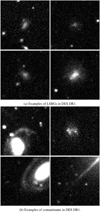 |
Fig. 1 g-band cut-outs of four examples of LSBGs (panel a) and con taminants (panel b) used in the training data. Each cut-out corresponds to a 40″ × 40″ (152 × 152 pixels) region of the sky centred on the LSBG or artefact. |
2.2 HSC data of Abell 194 cluster
The HSC is an imaging camera covering an area of 1.77 degree2 situated at the prime focus of the Subaru telescope with a pixel scale of 0.168″ (Bosch et al. 2018; Furusawa et al. 2018; Kawanomoto et al. 2018; Miyazaki et al. 2018; Komiyama et al. 2018). The Abell 194 cluster was observed with HSC using the HSC-g and HSC-r2 filters in a single pointing with dithered exposures. The r2 filter is an improved version of the r filter (Kawanomoto et al. 2018) and is referred to simply as the r-band throughout the text from this point onwards. The r-band observations were conducted on October 3, 2016, and the g-band observations took place on December 24, 2016. The dithering pattern was optimised to ensure that gaps between CCDs do not overlap in many exposures. Each dithered integration (referred to as a “visit”) began with the rotator angle set to 0 degrees to maintain consistent flat patterns near the edge of the field of view. The typical seeing size, represented by the full-width at half maximum (FWHM) of the point spread function (PSF), was approximately 1″ during the observing runs. For easier data handling, the observed field was divided into square patches, each 12′ on a side (4200 × 4200 pixels), with a 17″ (100 pix els) overlap between adjacent patches. Hence resulting in a total of 94 patches.
The data were reduced using the HSC pipeline, hscPipe (Bosch et al. 2018) version 8.5.3, in a standard way. hscPipe is based on software developed for the LSST project (Ivezic et al. 2008; Jurić et al. 2017). Astrometric and photo metric calibrations were performed using the Pan-STARRS1 catalogue (Magnier et al. 2013; Chambers et al. 2016), which is the standard with the HSC pipeline.
To estimate the median surface brightness depth at 3σ for a 10″ × 10″ region for the HSC data, we followed the proce dure described by Román et al. (2020). We randomly selected 1000 sky apertures, each covering a 10″ × 10″ region, from each of the 94 tiles (totalling 94 000 apertures) and fitted the counts in each aperture with a Gaussian profile. The σ values from each 10″ aperture were used to estimate the surface brightness depth at the 3σ10×10 level for a 10″ × 10″ region using the relation. (Román et al. 2020):
 (1)
(1)
Here, pix is the pixel scale (0.168 arcsec/pix) of the HSC data, and ZP is the zero point of the HSC data, which is calibrated to 27.05 mag. We estimated the median surface brightness depth at 3σ for a 10″ × 10″ region to be 30.5 ± 0.2 mag arcsec−2 in g-band and 29.7 ± 0.2 mag arcsec−2 for r-band. Here, the error corresponds to the median absolute deviation. This is ~2 magnitude deeper than DES data which has a median surface brightness depth of  mag arcsec−2 in the g-band and
  mag arcsec−2 in the r-band (Tanoglidis et al. 2021b).
2.3 GALEX
The Galaxy Evolution Explorer (GALEX; Martin et al. 2005) is a NASA small explorer mission that imaged the sky in far-ultraviolet (FUV; 1344–1786 Å) and near-ultraviolet (NUV; 1771–2831 Å) bands. The telescope has a 1.25-degree field of view and a resolution with an FWHM of 4.2″ and 5.3″ for the FUV and NUV bands, respectively. Each pixel in the intensity map from the GALEX corresponds to 1.5″ in the angular scale (Morrissey et al. 2007).
For our analysis, we use the intensity maps of all the available GALEX data within a 2-degree search radius of the Abell 194 cluster from the MAST database6. The intensity maps that par tially overlap were coadded using their corresponding exposure maps with the reproject Python package. The final co-added image has a variable exposure along the field of the Abell 194 cluster with a median exposure time of 4274 ± 1232 seconds in the NUV and 3943 ± 1393 seconds in the FUV band, where the error denotes the median absolute deviation.
3 Methodology
3.1 Transformer models
Transformers are DL models that use the attention mechanism to analyse correlations within input features for predictions or deci sions (Vaswani et al. 2017). In this work, we employ two types of transformer models: LSBG Detection Transformers (LSBG DETR) and LSBG Vision Transformers (LSBG ViT). These architectures were previously used for identifying LSBGs in DES DR1 by Thuruthipilly et al. (2024b). Here, we apply the same models to HSC data of the Abell 194 cluster, enabling a direct comparison with the results from Thuruthipilly et al. (2024b). Details about the training process can be found in Appendix A.1, and the performance of the individual models on the DES data is described in Appendix A.2. A compre hensive discussion of the transformer models is available in Thuruthipilly et al. (2024b).
3.2 Transfer learning
Generally, transfer learning refers to the practice of re-using a pre-trained model for a new task. In this work, we test transfer learning using the transformer models presented in Thuruthipilly et al. (2024b). These transformer models are trained to classify LSBGs and contaminants from the DES data (Sect. 2.1). We apply these models to a deeper dataset of the Abell 194 clus ter observed with HSC. This dataset is two magnitudes deeper than the training data and has a different resolution compared to DES. Our goal is to evaluate how well the transformer models can distinguish LSBGs from contaminants in this deeper dataset.
When using transfer learning between surveys, it is impor tant to adjust for differences in the instruments, as these cause variations in photometric zero points, pixel scales, and FWHM of PSF. For example, observing the same sky area with two instruments with different zero points and pixel scales will pro duce images with different pixel values in count units. For a DL model, the input parameter space (in this case, pixel values) is crucial for ensuring good model performance. Hence, a model trained on one survey could not be directly used on another survey and needs standardisation.
To standardise the data, we converted the pixel values of the images from counts per second to surface brightness units. This ensures that the average pixel values over a region remain con sistent, enabling direct comparison and standardisation of image data at the same wavelength across different surveys. Hence, before training and testing our transformer models, we converted each pixel value to its surface brightness (µJy arcsec−2) for DES DR 1 and HSC data, respectively.
However, it is important to note that this standardisation of data does not address the difference in PSF values between dif ferent surveys. It should be noted that we apply this conversion only for the application of the ML models, and all the measure ments and subsequent analysis are done on the original data.
3.3 Object detection and pre-selection of LSBG candidates in Abell 194
First, we generated a master catalogue of LSBG candidates by running SExtractor (Bertin & Arnouts 1996) on the image patches of the HSC data. Since the r-band was expected to better trace the mass distribution of LSBGs compared to the g-band, we used sky-subtracted r-band images for detection. However, for comparing with prior LSBG and UDG catalogues in Abell 194 (Tanoglidis et al. 2021b; Zaritsky et al. 2023; Thuruthipilly et al. 2024b), which used a g-band definition, we adopted their definitions for consistency. For source detec tion, we set the DETECT_THRESH to 1.5σ (~30.5 mag arcsec−2 for r-band) and DETECT_MINAREA to 49 pixels (~1.38 arcsec2), with these conservative values chosen to ensure all LSBGs are included.
We further applied selection cuts on the output catalogue based on the  , and the q as measured by the SExtractor to reduce the LSBG candidate sample. Since we are looking for extended LSBGs, we removed the bright and point objects from the full catalogue. The selection cuts applied to create the initial LSBG candidate sample are as follows:
We set
 to be in the range of 24.0 to 31.0 mag arcsec−2. The brighter limit is 0.2 magnitudes brighter than our LSBG definition to ensure no faint LSBGs are excluded. The faint end limit is fainter than the 3σ surface brightness detec tion threshold of the HSC data to ensure the preliminary catalogue includes all potential faint LSBGs.
reff,g was restricted to 2″ < reff,g< 20″, with the lower limit relaxed to maximise the detection of extended LSBGs. At the distance of Abell 194, this corresponds to 0.73 kpc < reff,g <7.3 kpc.
The axis ratio q (B_IMAGE/A_IMAGE) was set in the range 0.3 < q ≤ 1.0, following Greco et al. (2018) and Tanoglidis et al. (2021b). This removes contaminants such as highly elongated- diffraction spikes.
We removed the known foreground and background sources based on the redshift from SDSS Data Release 16 (SDSS DR16; Ahumada et al. 2020).
For each remaining source, we generated cut-outs in g and r-bands. Each cut-out is a 40″ × 40″ (238 × 238 pixels) region of the sky and is centred on the source. For sources near the edges of patches, we co-added the overlapping regions from nearby patches to obtain a 40″ × 40″ cut-out. To classify the cen tral source in each cut-out as an LSBG or artefact, we re-sized the HSC data cut-outs from 238 × 238 pixels to 64 × 64 pix els to match the input size of the transformer models. Similar to the DES data, the cut-outs in each band were re-sized using the Python package skimage.transform. The re-sized g- and r-band cut-outs were stacked for testing with the models. How ever, the re-sized cut-outs were used only for model testing, while the original cut-outs were utilised for Sérsic fitting, visual inspection, and aperture photometry.
3.4 Masks
Compact objects on top of LSBGs can influence the accuracy of Sérsic profile fitting (as discussed in Sect. 3.5). To obtain precise Sérsic parameters, we masked these objects following the proce dures outlined by Bautista et al. (2023). We ran the SExtractor on each cut-out three times by adjusting the control parameters to detect different types of contaminants, such as the bright sources, the faint sources lying outside the LSBG, and the faint sources lying on top of the LSBG. The CHECKIMAGE image that contains only the detected objects was used to create the masks for each kind of object, and all three masks were combined to create the final mask.
The first step is to remove the bright objects from the cut outs. The bright objects can be removed by setting a higher detection threshold without any limits on the size. We set DETECT_THRESH as 23.0 mag arcsec−2 and masked all the bright pixels. The second step is to remove faint, small objects that are far from the central LSBG. For this, we set a maximum area threshold (DETECT_MAXAREA) of 200 pixels at a detection threshold of 27.5 mag arcsec−2.
To identify smaller objects on top of LSBGs, we used the unsharp masking technique described in Bautista et al. (2023). This involves smoothing the original g-band image by convolv ing it with a Gaussian kernel, then subtracting the smoothed image from the original. After subtraction, features with sizes similar to or smaller than the smoothing kernel remained in the subtracted images. SExtractor was then used to detect and remove these small objects with an optimal configura tion of FWHM of the Gaussian kernel and DETECT_MAXAREA. The combination of these parameters varies depending on the sizes of the LSBGs and the overlapping small objects. While most masks (~40%) were created using FWHM = 2.0″ and DETECT_MAXAREA = 200, the same configurations can lead to poor masks for certain LSBGs. Through trial and error, we determined that using FWHM values of [2.0″, 1.25″, 2.50″] and DETECT_MAXAREA values of [200, 100] can produce accurate masks. Notably, the masks used in this study are more accurate than those from Tanoglidis et al. (2021b) and Thuruthipilly et al. (2024b), as they did not follow the same approach.
3.5 Sérsic fitting
We used GALFIT (Peng et al. 2010) to fit a single-component Sérsic profile to the sources identified as LSBGs by the trans formers in order to re-evaluate their  and reff,g. We opted for a single-component Sérsic fitting to align with the methodol ogy of Tanoglidis et al. (2021b) and Thuruthipilly et al. (2024b). However, it should be noted that Sérsic fitting may not always capture the complete light profile of a galaxy.
Since an error in the sky determination will significantly impact the Sérsic parameters, we subtracted the local sky from each cut-out prior to the Sérsic fitting (Bautista et al. 2023). The local sky is estimated as 2.5× median − 1.5× mean of the flux from the masked cut-out. However, if the median is greater than the mean, then the mean is treated as the local sky back ground (Da Costa 1992). Similar to Bautista et al. (2023), when calculating the total flux from each cut-out, a circular region of 10″ centred on the LSBG candidate, in addition to the masked region, is excluded to avoid including the light from the LSBG. The PSF image is generated by running PSFEX version 3.22.1 (Bertin 2013) on the patch from which the cut-out is taken.
The g-band images were fitted first. We used the MAG_AUTO and FLUX_RADIUS (with PHOT_FLUXFRAC=0.5) values obtained from the SExtractor as an initial guess for m and reff. We also used A_IMAGE and B_IMAGE to calculate the initial axis ratio q (B_IMAGE/A_IMAGE), which was allowed to vary in the range of 0.3 < q ≤ 1.0. The Sérsic index (n) was initialised at 1 and was allowed to vary only within the range of 0.2 < n < 5.0. The position angle was initialised at 90 deg and was allowed to vary without any restrictions to find the optimal angle. The ini tial centre was set at X = 119 pixels and Y = 119 pixels, which was allowed to vary ±5 pixels (0.84″) in both directions. These con ditions for the Sérsic fit were based on Greco et al. (2018) and Tanoglidis et al. (2021b). An example of an LSBG fitted with GALFIT is shown in Fig. 2. During the r-band fitting, we fixed the parameters X, Y, n, q, and PA to the values obtained from the g-band fitting, allowing only the magnitude and radius to vary.
After the fitting, we excluded all the sources with poor or failed fits with a reduced χ2 > 3. We excluded cases where the estimated n, q, X, and Y values did not converge or were at the edge of the specified range, as most of these objects (~90%) were later found to be contaminants. For the remaining galaxies, we re-applied our g-band sample selection criteria of  mag arcsec−2 and reff > 2.5″. The
  and µ0 values were calculated using the relations (Graham & Driver 2005):
 (2)
(2)
and
 (3)
(3)
where b is defined as 2γ(2n, b) = Γ(2n). Here, Γ and γ repre sent the complete and incomplete gamma functions, respectively, and the parameters were obtained from GALFIT. For all our measurements, we also applied a foreground galactic extinc tion correction using the Schlegel et al. (1998) maps normalised by Schlafly & Finkbeiner (2011) and a Fitzpatrick (1999) dust extinction law.
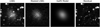 |
Fig. 2 Image of an LSBG (RA = 21.82879°, Dec = −1.81381°) as observed in HSC in the g-band, the image with all the objects other than LSBG masked, corresponding Sérsic model fitted by GALFIT and the residual are shown, respectively, from left to right. |
3.6 Visual inspection
We used visual inspection as the final step to improve the purity of the sample. However, for upcoming large-scale surveys like LSST, visual inspection may not be feasible due to the volume of data. In such cases, alternative approaches, such as accepting a sample with low contamination (5%) or using crowd science, may be necessary. Here, we considered candidates identified by either the LSBG DETR or LSBT ViT models and those that met the LSBG selection criteria with the updated GALFIT parame ters for visual inspection. This refined sample was independently visually inspected by two authors.
To aid in visual inspection, we used the colour images of the LSBG candidate downloaded from the DESI Legacy Imag ing Surveys Sky Viewer (Dey et al. 2019) as well as the g-band images from the HSC. Furthermore, the g-band Sérsic models from GALFIT were also inspected visually to ensure the quality of the fits. Each candidate was then categorised into three classes based on the GALFIT model fit and the image: LSBG, non-LSBG (contaminants), or misfitted LSBGs. If both visual inspectors agreed that the created masks and the resulting Sérsic model were accurate, the source was classified as an LSBG. However, if one visual inspector deemed the masks inaccurate or the Sérsic model’s radius did not match the source, it was classified as a misfitted LSBG and refitted with different initial conditions or improved masks. Finally, if the candidate did not look like an LSBG, we classified it as a contaminant or non-LSBG.
3.7 Aperture photometry
As was mentioned above, Sérsic fitting cannot always capture the complete light profile of a galaxy. Hence, we performed aperture photometry using photutils7 to estimate the apparent magni tude within a circular aperture of radius 8″ (~2.9 kpc) in the g, r, NUV and FUV bands. The aperture size was selected based on the maximum of the half-light radius distribution from GALFIT. This ensures that the size of the LSBGs is always smaller than the aperture size.
The masks used for the Sérsic fit were also applied in the aperture photometry. However, since the resolution of the NUV and FUV data (5″) is larger than the size of most LSBGs, we unmasked point objects overlying the LSBGs to avoid unneces sarily masking the data. These masks, originally created from the g-band images, were re-sized to match the pixel scale of the GALEX data. For NUV and FUV photometry, the error from the sky background is estimated by choosing an annulus with an inner radius of 10″ and an outer radius of 20″ and estimating the sky background from this region. Only sources with S /N > 3σ were considered as a confident detection, and for the cases with S /N < 3σ, the 3σ value was used to report the upper limit for the NUV and FUV magnitude. The aperture magnitudes were cor rected for foreground Galactic extinction, similarly as discussed in Sect. 3.5.
4 Results
4.1 Search for LSBGs with HSC in the Abell 194 cluster
By running the SExtractor patch by patch with the parameters specified in Sect. 3.3, we identified 170 328 sources. To reduce the sample size, we applied the selection criteria mentioned in Sect. 3.3. After applying the selection cuts to  , and q, we have 991 sources detected from Abell 194, which could be a potential LSBG. However, a large fraction of these sources are likely to be instrumental or physical contaminants rather than true LSBGs.
After applying the preselection as described in Section 3.3, we have a crude candidate catalogue of LSBGs. Further, we cross-matched the crude catalogue with SDSS DR 16 catalogue (Ahumada et al. 2020) to remove the foreground and back ground galaxies compared to the Abell 194 cluster. We identified 14 galaxies with known redshifts that do not match the redshift of Abell 194 (z = 0.0178), and these were removed from the sam ple. This reduced the size of the crude catalogue to 977 objects. The remaining objects in this catalogue could be an LSBG, an artefact, or a non-LSBG (a faint galaxy but not faint enough to be classified as an LSBG as per the definition that we use in this work).
To separate faint galaxies from contaminants, we applied our LSBG DETR and LSBG ViT models separately to all the objects that passed the selection criteria. The LSBG DETR mod els identified 258 LSBG candidates, and the LSBG ViT models identified 261 LSBG candidates independently. Among these, only 247 sources were classified as LSBG candidates by both models. To maximise the number of LSBGs, an input classified as an LSBG by either one of the ensembles is treated as an LSBG candidate and passed on for the subsequent analysis. Combining the outputs from both samples resulted in 272 LSBG candidates, which all underwent single-component Sérsic profile fitting using GALFIT. After the fitting, we re-applied the selection crite ria to screen the LSBG candidates. We applied selection cuts to the n, q, and centre positions X and Y of the fitter parameters as described in Sect. 3.5. These criteria were used to eliminate any poor fits and contaminants, if present. Two of the authors inde pendently visually inspected the masks and fitted galaxy profiles to ensure the quality of the fit. Finally, we had 159 LSBGs, with 11 detected by only the LSBG ViT ensemble model.
To estimate the number of the LSBGs missed by our model, we also repeated the GALFIT and visual inspection of all the 705 objects rejected by the ensemble models. This was done to estimate the number of FNs predicted by the model and to min imise their occurrence in the future by understanding why they were missed. Our model missed 12 LSBGs, making the total number of LSBGs around Abell 194 to 171. Thus, our model achieved a true positive rate (TPR) of ∼93% on the HSC dataset without any fine-tuning. The schematic diagram showing the sequential selection steps used to create LSBGs and UDGs in Abell 194 is shown in Fig. 3. A sample catalogue comprising the properties of the identified LSBGs in this work is shown in Table B.1. Six examples of LSBGs and UDGs identified from our study are shown in Fig. 4.
Girardi et al. (1998) and Rines et al. (2003) have estimated the comoving radius of Abell 194 as 0.69 h−1 Mpc. Plugging in the cosmological parameters, we calculate the virial radius, r200 of Abell 194 to be 0.9824 Mpc. 12 among the 171 LSBGs are located slightly beyond the virial radius of the cluster, with the most distant LSBG being 1.15 Mpc away from the cluster cen tre. However, since LSBGs and UDGs have also been observed outside the virial radius in other clusters (Venhola et al. 2018, 2022; Junais et al. 2022), for simplicity, we treat all 171 LSBGs as part of the Abell 194 cluster. Based on the redshift of Abell 194, 28 of the 171 identified LSBGs, with reff,g > 1.5 kpc and µ0,g > 24.0 mag arcsec−2, are classified as UDGs. Only 2 of these 28 UDGs were missed by the ML models and required visual re-identification, consistent with a TPR of 93%.
The distribution of the g-band magnitudes of LSBGs and UDGs is shown in Fig. 5a. The UDGs have a median g-band magnitude of 20.2 ± 0.5 mag, which is brighter than the median value of 20.7 ± 0.6 mag for the LSBGs. Here, the median abso lute deviation represents the error associated with the median. This suggests that our sample includes very faint LSBGs that are not large enough to be classified as UDGs. The distribution of the Sérsic index (n) for LSBGs and UDGs is shown in Fig. 5b. The Sérsic index for LSBGs predominantly lies between 0.5 and 1.5, with a median value of 0.87 ± 0.14. In contrast, the UDGs have a Sérsic index distribution with a median of 0.72 ± 0.09, which is slightly lower than that of the LSBGs. A detailed dis cussion of the properties of the LSBGs and UDGs identified in this work is presented in Sect. 5.
As was discussed in Sect. 3.7, aperture photometry pro vides a more reliable estimate of apparent magnitude. We esti mated the apparent magnitudes in the g, r, NU V , and FU V bands, applying corrections for galactic extinction as outlined in Sect. 3.7. 20 LSBGs in our sample had confident detections in NUV (S/N > 3σ), whereas only 15 LSBGs had confident detec tion in the FUV. For the rest of the sample, we estimated the upper limits of the NUV and FUV magnitude based on their 3σ values within the aperture. The aperture magnitudes were used to estimate the colours g − r, NUV − r, and FUV − NUV. The aperture magnitude of the r-band was used to estimate the absolute magnitude (Mr) in the r-band. Using the stellar mass-to-light ratio vs colour relation for LSBGs from Du et al. (2020), we estimated the stellar masses (M⋆) of our sample based on their aperture g-r colour. Similarly, the stellar mass surface density (Σ⋆) was calculated using the stellar mass-to-light ratio and the mean surface brightness  in the r-band, following Eq. (1) of Chamba et al. (2022). A detailed discussion of the physical and cluster-centric properties of the LSBGs and UDGs identified in this study is provided in Sect. 5.
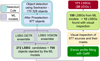 |
Fig. 3 Schematic diagram showing the sequential selection steps used to find the LSBGs and UDGs in Abell 194. |
4.2 Transformers for cross-survey LSBG detection
Here, we explore the effectiveness of transfer learning for iden tifying LSBGs in the HSC dataset using transformer models from Thuruthipilly et al. (2024b) trained on DES DR1. On the HSC dataset, they correctly identified 159 of 171 LSBGs, with a 93% TPR, without fine-tuning. This demonstrates the potential of transfer learning with transformer models.
Although the model missed 12 LSBGs, which is a small fraction of the total (∼7%), it is important to closely examine these missed cases to enhance model performance in the future. The magnitude distribution of the LSBGs in the training data, LSBGs identified and missed by the models, are presented in Fig. 6. Here, the magnitude distribution of the training sample and LSBGs identified by the ensemble models share the same lower limit (g ~ 22.5 mag). However, only ~1.7% of LSBGs in the training data have 21.5 < g < 22.5. Consequently, 9 out of the 12 missed LSBGs had g < 21.5 mag and the performance of the models in identifying LSBGs with g > 21.5 mag is sub-optimal. This suggests that the inability of the model to identify them was due to the underrepresentation of such faint LSBGs in the training data. Nevertheless, potentially, one could refine the ensemble models by retraining them with very faint LSBGs (g > 21.5 mag) from simulations or small-scale deep surveys, thereby extending the models’ performance to a fainter regime.
Similarly, analysing the other 3 LSBGs missed by the ensem ble model, which had g < 21 mag, it was found these galaxies were very close to a bright galaxy. This caused the model to confuse them as part of a bright galaxy and classify them as a non-LSBG. The presence of very bright objects introduces a bias in the prediction probabilities of the ensemble models, and it was also found that the effect is greater if the bright object is close to the centre of the cut-out. Examples of the LSBGs missed by the model are shown in Fig. 7.
A total of 101 objects initially classified as LSBGs were reclassified as non-LSBGs after further analysis using GALFIT and visual inspection. The rejected sample predominantly com prised three types of objects: faint galaxies that did not meet the LSBG criteria, with  in the range 24.0–24.2 mag arcsec−2 and reff,g between 2″ and 2.5″ (approximately 60%), very faint blended sources (about 10%), and instrumental contaminants from HSC (around 30%). Simple selection cuts on the morpho logical parameters can remove the first class. Similarly, the third class of objects could be removed by having a representative of instrumental contaminants in the training set. Alternatively, applying selection cuts based on the convergence of the Sérsic fit reduces these contaminants, as most do not converge. The sec ond class of contaminants are generally very faint and are hard to remove. While their numbers are small compared to LSBGs, they still require visual inspection. Notably, even human inspec tors will have trouble distinguishing these faint blended sources from LSBGs. For instance, 14 of the 17 sources where the two authors disagreed during independent visual inspection had
  mag arcsec−2.
Large-scale surveys like LSST and Euclid are expected to detect 105 + LSBGs, necessitating efficient methods to analyse large volumes of data. Successful implementation of transfer learning will be pivotal in this effort, allowing the applica tion of knowledge from existing datasets to process data from upcoming surveys effectively. Models with high TPR will ensure better completeness by capturing a larger fraction of genuine LSBGs, while low false positive rates (FPR) will enhance sam ple purity by minimising contamination. Generally, TPR and FPR should be balanced based on the classification problem. In unbalanced datasets, reducing FPR is key, while maximising TPR helps when contaminants can be pre-filtered. Furthermore, advanced ML methodologies will be essential for addressing the challenges posed by the scale and complexity of future datasets.
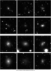 |
Fig. 4 Top panel (a): shows six examples of LSBGs identified from our study. Bottom panel (b): shows six examples of UDGs identified from our study. Each cut-out of the LSBG and UDG corresponds to a 40″ × 40″ (152 × 152 pixels) region of the sky centred around the LSBG or the UDG in the g-band. |
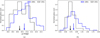 |
Fig. 5 Normalised distributions of the g-band magnitude and Sérsic index for the LSBGs and UDGs identified from HSC data in this study are shown in the left (a) and right (b) panels, respectively. The long black arrow shows the median of the UDG distribution, and the shorter blue arrow shows the median of the LSBG distribution in both plots. |
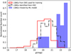 |
Fig. 6 Normalised distribution of g-band magnitudes for the LSBGs used to train the ensemble models, LSBGs identified by the ensemble models in the HSC data of the Abell 194 cluster, and LSBGs missed by the ensemble models in the HSC data of the Abell 194 cluster. |
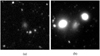 |
Fig. 7 Example g-band images of LSBGs missed by the ensemble mod els. The left panel shows an LSBG, which is fainter than the training sample, and the right panel shows an LSBG near bright galaxies. |
5 Discussion
5.1 Comparison with previous catalogues of LSBGs and UDGs in Abell 194
In total, Tanoglidis et al. (2021b) and Thuruthipilly et al. (2024b) identified 96 LSBGs in Abell 194, which we call the LSBGs-DES sample. Among these, 19 LSBGs could be classified as UDGs based on their reff,g and µ0,g measured from DES. Similarly, Zaritsky et al. (2023) identified 14 UDGs in Abell 194, with 9 overlapping both the LSBGs-DES sample and the subset of 19 UDG candidates from LSBGs-DES. In our final sample, the ensemble model identified 13 UDGs from Zaritsky et al. (2023). One missing UDG was found later when reviewing the rejected sources. Similarly, 95 out of 96 from the LSBGs-DES sample were re-identified by the ensemble model. One LSBG, missed by the model, was subsequently found during visual inspection.
However, the final catalogue contains only 84 LSBGs from the LSBGs-DES sample. The remaining 12 were reclassified as non-LSBGs: 11 galaxies were slightly brighter  than our threshold, and one LSBG was found to have a higher redshift (z=0.15) when cross-matched with the SDSS DR 16 sample. Additionally, 7 UDG candidates based on DES measurements were reclassified as non-UDGs due to having a physical radius smaller than 1.5 kpc, and one due to a µ0,g brighter than 24.0 mag arcsec−2. Similarly, 2 UDGs from Zaritsky et al. (2023) were reclassified as non-UDGs, which was also a subset of the LSBGs-DES sample: one due to a µ0,g brighter than 24.0 mag arcsec−2 , and the other due to a physical radius smaller than 1.5 kpc.
One of the primary reasons for rejecting some LSBGs and UDGs from previous catalogues is the improved masking strat egy implemented in this study. These improved masks effectively removed small contaminants overlaid on the galaxies, as shown in Fig. 2. In shallow data, these contaminants might not be clearly visible, but with deeper data, these contaminants are clearly visible and significantly affect the estimation of the mor phological parameters such as Sérsic index and half-light radius during a Sérsic fit. The measurements from DES were performed without masking the contaminants that may reside on top of the LSBGs. As these contaminants are very compact objects, the presence of these contaminants tends to increase the Sérsic index of the LSBG during fitting. Similarly, because of the addi tional light from these contaminants, the reff,g of these galaxies also tends to be over-estimated. However, the presence of these contaminants does not significantly affect the magnitude of the galaxy. These trends were also observed by Bautista et al. (2023) for the estimated Sérsic parameters of UDGs from the Coma cluster.
An additional factor contributing to the deviation in the Sérsic parameters between this study and those reported by DES is the local sky subtraction. Previous searches for LSBGs in DES by Tanoglidis et al. (2021b) and Thuruthipilly et al. (2024b) did not consider the local sky subtraction. The sky background in publicly available DES data is estimated with regions of size ∼1′ (Morganson et al. 2018; Bernstein et al. 2018). This is considerably larger than the size of the LSBGs we investi gate in this work. Sky subtraction over a large area tends to over-subtract the sky due to the influence of bright objects. This can result in LSBGs appearing fainter than their actual surface brightness. Hence, failing to correct for local sky subtraction can lead to inaccurate Sérsic fits, as also highlighted by Bautista et al. (2023).
Despite excluding some LSBGs from the previous DES sam ple, the number of LSBGs in the Abell 194 cluster has increased from 84 to 171. This rise is partly due to the deeper sensi tivity of the HSC data, which is two magnitudes deeper than DES, but not solely because of it. Preselection criteria applied with SExtractor also played a significant role. For instance, the ratio of reff,g estimated by SExtractor to GALFIT has a median value of 0.8, indicating that SExtractor underestimates the radius. A similar ratio was found in the LSBG sample by Tanoglidis et al. (2021b). As a result, we relaxed our preselec tion to FLUX_RADIUS_G >2.0″, compared to the >2.5″ threshold used by Tanoglidis et al. (2021b) and Thuruthipilly et al. (2024b). Without this adjustment, only 25 new LSBGs would have been identified, which is a 30% increase. For UDGs, preselection had less impact, as only 3 of 28 UDGs had a FLUX_RADIUS_G between 2–2.5″. However, if the cluster were slightly farther away (z ≳ 0.025), the preselection effects would become signif icant, as the angular size of a UDG would approach 2.5″.
The radar plot comparing the properties of the LSBGs-DES sample and the new LSBGs identified with HSC in Abell 194 is shown in Fig. 8. In terms of colour (g − r), q and n, both samples have the same median, indicating that both samples are similar in these properties. As was mentioned earlier, the new sample of LSBGs has many small LSBGs in size, which is evident from the median values of the LSBGs detected from DES (1.4 ± 0.2 kpc) and not detected in DES (1.1 ± 0.1 kpc). Similarly, as expected, the new sample of LSBGs is fainter than the LSBGs-DES sample. This is evident from the median values of  , µ0,g, logΣ★, logM⋆ , and raperture when comparing LSBGs detected in DES to those not detected in DES.
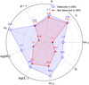 |
Fig. 8 Comparison of morphological and physical properties of LSBGs identified from DES and the LSBGs identified only in HSC. The median of g – r (mag), q, n, reff,g (kpc), |

5.2 Properties of the LSBG and UDG population of the Abell 194 cluster
As mentioned in Sect. 1, UDGs are a subclass within LSBGs, characterised by their extended half-light radii (re ≥ 1.5 kpc) and high central surface brightness (µ0 > 24 mag/arcsec2) in the g- band (van Dokkum et al. 2015a). Assuming all the LSBGs in this work share the same redshift as Abell 194, we estimate that our sample has 28 UDGs and 143 non-UDGs. However, some may be foreground or background galaxies, and individual redshifts are required to confirm their UDG status.
5.2.1 Abundance of UDGs
Since van Dokkum et al. (2015a) found a substantial population of UDGs within the Coma cluster, the subsequent studies have identified numerous UDGs in various galaxy clusters (Koda et al. 2015; Yagi et al. 2016; Mihos et al. 2015; Lim et al. 2020; La Marca et al. 2022; Bautista et al. 2023). Further investigations have demonstrated that not only clusters, groups are also abundant with UDGs (Merritt et al. 2016; Román & Trujillo 2017; Müller et al. 2018; Somalwar et al. 2020; Forbes et al. 2020) and their abundance has a near-linear correlation in the log scale with the mass of the dark matter halo of the cluster (van der Burg et al. 2017; Mancera Piña et al. 2018; Karunakaran & Zaritsky 2023). Karunakaran & Zaritsky (2023) estimated that the number of UDGs scale as a function of the halo mass following the relation  . For the Abell 194 cluster, which has a halo mass of 7.6 × 10¹³M⊙, this relation predicts 30 ± 4 UDGs. The number of UDGs as a function of host halo mass, including Abell 194, is shown in Fig. 9.
However, since the UDG definition in the literature is not unique, the sample used by Karunakaran & Zaritsky (2023) is brighter ( mag arcsec−2) than our UDG sample which has µ0,g > 24.0 mag arcsec−2. Using the same definition as Karunakaran & Zaritsky (2023), we identified 45 LSBGs that meet the criteria to be considered UDGs, referred to as the ’relaxed’ UDG sample. This number exceeds the value predicted by Karunakaran & Zaritsky (2023), as shown in Fig. 9. As our primary objective does not focus on constraining the relationship between halo mass and the number of UDGs, we do not re-calibrate this relation and have reserved it for potential future work.
5.2.2 UDG surface number density
The spatial distribution of the UDGs in the clusters can be used to probe how the environment affects the formation of the UDG population. The radial surface density profile of UDGs from Abell 194, as well as the UDGs from the literature, is shown in Fig. 10. Given that more massive clusters tend to host a greater number of UDGs, as indicated in Fig. 9, we normalised the radial surface density of each cluster by its mass to standardise the comparison of UDG distributions across different clusters. In addition, since the UDG definition in the literature is not unique, we selected the UDG samples in each cluster based on the definition used by van Dokkum et al. (2015a).
The normalised surface number density distribution of UDGs in the cluster follows the same trend as shown in Fig. 9. Since the number of UDGs scales with cluster mass, the surface number density normalised by cluster mass remains consistent across different clusters, as evident in Fig. 10. Furthermore, the spatial variation in the normalised UDG surface number density is uniform beyond 0.3R200 for various clusters. However, near the cluster centre, the values show variation, indicating that UDG formation in the inner region is influenced by factors other than halo mass. A more detailed study is needed to identify these additional factors.
We also observe that the Abell 194, Hydra (La Marca et al. 2022), and Virgo (Junais et al. 2022)8. Clusters exhibit similar normalised UDG surface number density distributions near the cluster centre (<0.3R200), suggesting that UDG formation in these clusters may follow a similar pattern. However, further investigation and follow-up studies are needed to confirm this. In contrast, the Fornax cluster (Venhola et al. 2018, 2022) shows a decline in the normalised number density near the cluster centre, which could indicate that UDGs either do not survive in the inner region of the Fornax cluster or they have not been detected yet.
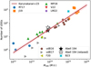 |
Fig. 9 Number of UDGs as a function of halo mass, includes data from various studies. Cluster UDGs are represented by brown hexagons (van der Burg et al. 2016), orange squares (Janssens et al. 2019), upward green triangles (Mancera Piña et al. 2019), downward red triangles (Venhola et al. 2022), purple pentagons (La Marca et al. 2022), and cyan crosses (Bautista et al. 2023). Group UDGs are represented by grey right-pointing triangles (van der Burg et al. 2017), blue circles (Román & Trujillo 2017), and left-pointing olive triangles (Forbes et al. 2020). The UDGs reported in this work are shown as a black star, while the UDG sample with a relaxed definition, similar to Karunakaran & Zaritsky (2023), is represented by a hollow black star. |
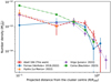 |
Fig. 10 Radial surface density profile of cluster UDGs, normalised by cluster mass (M200), as reported in this work and the literature. The UDGs are from Venhola et al. (2018, 2022) (Fornax; blue circles), La Marca et al. (2022) (Hydra; orange triangles), Junais et al. (2022) (Virgo; purple rhombus), and Bautista et al. (2023) (Coma; green squares). |
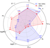 |
Fig. 11 Comparison of morphological and physical properties of UDGs and non-UDGs. The median of g – r (mag), q, n, reff,g (kpc), |

5.2.3 LSBGs versus UDGs
As the UDGs are considered a subclass of LSBGs, one might be curious about the difference in the properties of UDGs and non- UDGs (LSBGs that did not satisfy the condition to be a UDG). The radar plot comparing the median distribution of all the properties estimated in this work for the UDGs and non-UDGs is shown in Fig. 11. Comparing the median value of g – r colour, we can see that both UDGs (0.53 ± 0.04) and non-UDGs 0.55 ± 0.03 have a similar colour distribution. The median colour of the UDGs reported here is consistent with the median colour of the UDG sample presented in Mancera Piña et al. (2019) (0.59) and Bautista et al. (2023) (0.55). Similarly, in terms of axis ratio also, both the UDGs (0.72 ± 0.09) and non-UDGs (0.75 ± 0.14) have a similar distribution, indicating that they have a slightly elongated shape. Coming to the Sérsic index, the non-UDGs (0.88 ± 0.14) and UDGs (0.72 ± 0.09) have comparable median values. These values are comparable with the values reported for the UDGs in Mancera Piña et al. (2019) (0.96) and Bautista et al. (2023) (1.0).
The median reff,g for UDGs (1.8 ± 0.2 kpc) is larger than that of non-UDGs (1.2 ± 0.2 kpc), which is a consequence of the definition of UDGs. The UDGs also have fainter median µ0,g (24.6 ± 0.5 mag arcsec−2 vs 24.0 ± 0.5 mag arcsec−2) and  (25.1 ± 0.5mag arcsec−2 vs 24.3 ± 0.5 mag arcsec−2) compared to non-UDGs. The stellar mass surface density of UDGs (106.5±0.2 M⊙ kpc−2) is slightly lower than that of non-UDGs (106.8±0.2 M⊙ kpc−2). These trends in µ0,g,
  and M⊙ are consistent with the UDGs being fainter extended sources. However, UDGs have higher median total stellar mass and a brighter median apparent magnitude in the r-band, indicating they contain more stellar mass and emit more light, but their extended structure results in fainter surface brightness.
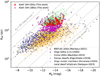 |
Fig. 12 The size-luminosity relation for local dwarf ellipticals, LSBGs, and UDGs from various studies is shown, with reff,g (in parsecs) on the y-axis and Mg (mag) in the g-band on the x-axis. Red crosses and magenta circles represent the LSBGs and UDGs from this work. Brown triangles, purple diamonds, and lime green squares indicate UDGs from the MATLAS survey (Marleau et al. 2021), the Virgo cluster (Lim et al. 2020), and the Coma cluster (Bautista et al. 2023). The blue circle marks the Fornax dwarf from Eigenthaler et al. (2018), orange stars represent local dwarf ellipticals from Paudel et al. (2023), and black pentagons show low-mass Virgo cluster members from Ferrarese et al. (2020). The grey lines represent constant surface brightness values, ranging from |


5.2.4 LSBGs, UDGs, and dwarf galaxies
The morphological parameters, such as the Sérsic index of LSBGs and UDGs, show a distribution similar to that of dwarf ellipticals reported by Poulain et al. (2021). Simulations further indicate that the dark matter halos of UDGs and dwarf galaxies have comparable masses (Amorisco & Loeb 2016; Di Cintio et al. 2017; Sales et al. 2020; Jiang et al. 2019; Benavides et al. 2023). These results suggest that the UDGs in our sample may simply be extended dwarf galaxies rather than a distinct population of galaxies.
Different galaxy populations can be distinguished by their structural parameters and scaling relations, which vary among galaxy families (Kormendy 1985; Kormendy et al. 2009). A comparison of the size-luminosity relations for local dwarf ellipticals (Eigenthaler et al. 2018; Ferrarese et al. 2020; Paudel et al. 2023) and UDGs (Lim et al. 2020; Marleau et al. 2021; Bautista et al. 2023) from the literature, along with the LSBG and UDG populations identified in this work, is presented in Fig. 12.
The overlap between dwarf galaxies and UDGs in the Reff − Mg plane suggests that UDGs are an extended subset of dwarf galaxies, occupying the diffuse, low-surface-brightness end of the size-luminosity relation. These findings also align with previous studies (Conselice 2018; Marleau et al. 2021; Wang et al. 2023; Bautista et al. 2023; Zöller et al. 2024). The UDGs from different clusters also occupy similar regions in this plane, indicating that their formation channels are likely consistent across clusters. Nonetheless, environmental factors may also play a role, as Coma, the most massive cluster, hosts the largest UDGs, while the Virgo cluster contains the faintest UDGs. Since these UDG samples are taken from different surveys, this conclusion may be biased by the surface brightness limits of these surveys as well.
The majority of LSBGs in our sample exhibit structural parameters similar to those of local dwarf galaxies, suggesting a close connection between these populations. This is further supported by the findings of Lazar et al. (2024), who observed that the red-to-blue fraction of dwarf galaxies closely mirrors that of LSBGs, reinforcing the idea that most LSBGs are indeed dwarf galaxies. Furthermore, the lack of a clear boundary in the sizeluminosity plane between dwarf galaxies, LSBGs, and UDGs implies that these populations may form a continuous spectrum rather than distinct classes.
 |
Fig. 13 Spatial distribution of LSBGs and UDGs in the Abell 194 cluster. The LSBGs identified in this work are shown as magenta circles, and UDGs from this work are shown as red crosses. The LSBGs identified in DES by Tanoglidis et al. (2021b) and Thuruthipilly et al. (2024b) are marked with dark green circles, and UDGs reported in Zaritsky et al. (2023) are represented by blue squares. The KDE highlights regions with varying concentrations of LSBGs, ranging from blue to red, with blue indicating areas of higher density. The dashed black circle, the black diamond, and the black dot represent the virial radius, the cluster centre, and NGC 519, respectively. |
5.3 Cluster-centric properties of LSBGs and UDGs
The spatial distribution of LSBGs and UDGs in the Abell 194, along with the spatial kernel density estimate (KDE) of LSBGs, is presented in Fig. 13. The KDE provides a smooth estimate of the density of these galaxies across the cluster, highlighting areas with higher concentrations of LSBGs. The Abell 194 has a tail of bright galaxies from the cluster centre to the direction of NGC 519, which are found to be falling towards the cluster centre (Tempel et al. 2016). The spatial density of LSBGs at the cluster centre aligns with the bright galaxies in the direction of NGC 519, suggesting that LSBGs may follow the bright galaxies toward the cluster centre and could be their satellite galaxies.
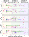 |
Fig. 14 Morphological and physical properties of LSBS and UDGs as a function of cluster centric distance. The x-axis shows the distance from the cluster centre in Mpc. The LSBGs and UDGs identified in this work are shown in magenta dots and red crosses, respectively. The running median of LSBGs and UDGs are calculated with a bin size of 0.4 Mpc and are represented as dashed blue and solid green lines, respectively. The inner, middle, and outer regions of the cluster are shaded with yellow, green, and blue, respectively. |
5.3.1 Trends in morphological and physical properties with projected cluster-centric distance
The projected distance can serve as a proxy for density within clusters and can be used to analyse how the environment affects the structural properties of an LSBG or UDG. The structural and physical properties of the LSBGs and UDGs as a function of the cluster-centric distance are shown in Fig. 14. To facilitate comparison, we assigned the area within a radius of less than 0.4 Mpc around the cluster centre as the inner region of the cluster, while the region beyond a radius of 0.8 Mpc is considered the outer skirts of the cluster. The region in between is considered the middle region of the cluster.
The median value of the Sérsic index shows no significant trend for both LSBGs and UDGs as a function of the clustercentric distance. Similarly, the median axis ratio of LSBGs tends to be relatively flat throughout the regions. In contrast, the median axis ratio of UDGs tends to be ∼0.6 ± 0.1 near the inner region of the cluster, increases to ∼0.7 ± 0.1 in the middle, and decreases again towards the outer region of the cluster. Our observations on the Sérsic index and axis ratio align well with the observations by Román & Trujillo (2017); Mancera Piña et al. (2019) and are in good agreement with expectations from models of dwarf galaxies that have undergone harassment and tidal interaction processes (Moore et al. 1996; Aguerri & González- García 2009).
The surface brightness distribution shown in Fig. 14 indicates that LSBGs and UDGs in the inner regions of the cluster are brighter than those in the middle region. The absence of faint LSBGs and UDGs in the inner regions could be due to the destruction of low-mass galaxies by the more massive galaxies at the cluster centre. Another possible reason for this could be the non-detection of the faint sources due to the contamination from the bright sources and the intra-cluster light. However, it should also be noted that the outer region of the cluster shows a lack of very faint LSBGs. A detailed follow-up study with improved methodology is necessary to confirm if this is a statistical bias or reflects a physical phenomenon.
The size distribution of UDGs in the cluster shows that UDGs in the inner and middle regions have similar sizes. In contrast, UDGs in the outer skirts of the cluster tend to be larger, potentially because they are already extended UDGs falling into the cluster. In terms of stellar mass distribution, UDGs in the inner region of the cluster had higher stellar masses than those in the middle and outer regions. In contrast, the running median for LSBGs remained flat across all the cluster regions.
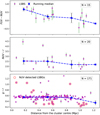 |
Fig. 15 FUV – NUV (top panel), NUV – r (middle panel) and g – r (bottom panel) colours of the LSBGs presented in this work as a function of cluster centric distance. The number of LSBGs used is also shown in each subplot since not all the LSBGs had 3σ detection in NUV and FUV bands. |
5.3.2 Trends in colour with projected cluster-centric distance
Recently, Venhola et al. (2019) found that the early type dwarf galaxy population in the Fornax cluster becomes redder as we go towards the cluster centre in the u – X (where X ∈ g, r, i) colour. The UDGs also have shown a similar trend in becoming bluer as going towards the outskirts of the cluster centre (Román & Trujillo 2017; Mancera Piña et al. 2019; Junais et al. 2022). The FUV – NUV, NUV – r and g – r colours of our sample as a function of the cluster centric distance are shown in Fig. 15.
We observe that LSBGs become progressively redder in FUV – NUV colour as they approach the cluster centre. The median FUV – NUV colour in the inner region of the cluster is approximately 0.5 mag redder than those in the outer region, suggesting that the LSBGs near the cluster centre in Abell 194 are quenched. Since FUV – NUV colour is sensitive to recent star formation history, this indicates that LSBGs on the outskirts may have undergone more recent star formation than those near the cluster centre. However, these conclusions are limited by the small sample size and should be confirmed with future studies.
Additionally, the median NUV – r colour shows a weak trend of becoming redder towards the cluster centre, though this trend is less pronounced than in FUV – NUV. Nonetheless, the reddest LSBGs in NUV – r are found in the inner cluster region, further supporting the idea that LSBGs near the centre of Abell 194 are quenched. Similar trends in UV-based colours have been reported by Venhola et al. (2019) and Junais et al. (2022).
In contrast, our sample of LSBGs shows no clear trend in g – r colour (which traces the old stellar population) with respect to cluster-centric distance up to 0.8 Mpc. However, LSBGs in the outer regions of the cluster appear bluer by 0.1 mag compared to those in the inner and middle regions. We also note that LSBGs with NUV detection in the inner region are redder in g – r colour than those in the middle and outer regions of the cluster.
Recently, Singh et al. (2019) studied the UV properties of UDGs in the Coma cluster using GALEX data and concluded that most UDGs in the cluster are quiescent, showing no signs of recent star formation. However, a subsequent analysis by Lee et al. (2020) suggested that some UDGs near the cluster centre may exhibit signs of recent star formation. In our sample, we also observed a few LSBGs near the cluster centre that had detectable UV emissions.
In Fig. 16, we compare the distribution of the LSBGs and UDGs from our sample and the UDGs from the Coma cluster from Singh et al. (2019) and Lee et al. (2020) in the colourmagnitude space (NUV – r vs Mr). In our sample, we have only one UDG with NUV detection, which belongs to the blue population. Similar to the population of Coma UDGs from Lee et al. (2020), we have four LSBGs belonging to the red population with NUV detection. It should also be noted that the population of LSBGs and UDGs in our sample are much fainter than the population of UDGs presented in Singh et al. (2019) and Lee et al. (2020).
6 Conclusion
In this paper, we explore the potential of transfer learning with the transformer models presented in Thuruthipilly et al. (2024b). We trained the transformer ensemble models on the LSBGs and contaminants from DES DR 1, which is presented in Tanoglidis et al. (2021b) and Tanoglidis et al. (2021a) and updated by Thuruthipilly et al. (2024b). Subsequently, the trained transformer models were applied to identify LSBGs from the data of the Abell 194 cluster, observed with HSC, which is two magnitudes deeper than DES DR1. Since the instrument used to image in DES DR 1 is different from the HSC, we standardise the data from both instruments by converting their units into surface brightness units (µJy arcsec–2).
After fitting Sérsic profiles and conducting visual inspections on the LSBG candidate sample identified by the transformer models, we identified 159 LSBGs. However, the transformer models failed to identify 12 LSBGs, which were found through visual inspection of the rejected sample. Among the 12 LSBGs missed by the ensemble models:
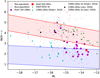 |
Fig. 16 NUV – r colour plotted against the absolute magnitude in the r-band. The red region denotes the space occupied by the red-quiescent galaxy population, while the blue region represents the blue galaxy population (Singh et al. 2019). Magenta dots represent LSBGs, and red crosses represent UDGs with NUV detection in our sample. Green stars indicate the upper limits of NUV – r for UDGs in Abell 194 without NUV detection. Upward cyan triangles and black plus symbols represent UDGs from the Coma cluster reported by Singh et al. (2019) and Lee et al. (2020), respectively. Downward navy blue triangles and pink rhombuses denote the upper limits of NUV – r for UDGs in the Coma cluster from Singh et al. (2019) and Lee et al. (2020), respectively. |
9 LSBGs are fainter than the training sample (g < 21.5 mag) and lack representation in the training set.
3 LSBGs have bright objects near their centres.
Thus, our final sample has 171 LSBGs, including 28 UDGs. The transformer models achieved a TPR of 93%, comparable to the 96% TPR obtained on the DES dataset (see Appendix A.2). The reported metrics, even without fine-tuning, confirm the success of transfer learning, suggesting these models could be effectively applied to deeper datasets from LSST and Euclid.
Tanoglidis et al. (2021b) and Thuruthipilly et al. (2024b) have identified 96 LSBGs in Abell 194, referred to as LSBGs- DES sample. Similarly, Zaritsky et al. (2023) identified 14 UDGs in Abell 194, among which 9 are part of the LSBGs-DES sample. From the deep data of Abell 194, our models identified 95 out of 96 known LSBGs and 13 out of 14 known UDGs. In this work, we found that improved masks and local sky subtraction significantly influence the parameters such as the Sérsic index, similar to the finding of Bautista et al. (2023). In the new sample, 12 LSBGs identified from the DES are not included as they are slightly brighter (0.1 mag) than our selection cut. In the final sample, we have:
84 LSBGs also detected in DES by Tanoglidis et al. (2021b) and Thuruthipilly et al. (2024b).
new 87 LSBGs identified with the deep HSC observations.
The newly estimated number of UDGs in Abell 194, based on data from the HSC, supports the argument in the literature that the number of UDGs in a cluster is linearly correlated with cluster mass on a log scale (van der Burg et al. 2017; Mancera Piña et al. 2018; Karunakaran & Zaritsky 2023). However, we found that the number of UDGs in Abell 194 exceeds the predicted value from Karunakaran & Zaritsky (2023). Since we lacked sufficient new data points to statistically refine the relation, further analysis was left for future work. Additionally, this relation may be influenced by the limiting magnitude of the surveys used to identify UDGs. In the future, we plan to account for the limiting magnitudes when constraining these relations. The surface number density of UDGs, normalised by cluster mass, is consistent across different clusters, further indicating that UDG abundance is correlated with cluster mass.
The Sérsic index distribution of the UDGs in this work is consistent with values reported in the literature (Koda et al. 2015; Yagi et al. 2016; Román & Trujillo 2017; van der Burg et al. 2017; Venhola et al. 2022; Bautista et al. 2023; Thuruthipilly et al. 2024b). Additionally, the Sérsic index distribution of UDGs is similar to that of dwarf elliptical galaxies, with UDGs occupying the diffuse, low-surface-brightness end of dwarf galaxies in the Reff – Mg plane. This suggests that UDGs may be an extended subset of the dwarf galaxy population.
No significant trends in n are observed for LSBGs and UDGs as a function of the cluster-centric distance. The LSBGs and UDGs near the cluster centre tend to be brighter, and there is an under-representation of faint LSBGs in the outer parts of the cluster, which needs further investigation.
Applying aperture photometry to the available GALEX data of Abell 194, 15 LSBGs in our sample show confident detections (S/N ≥ 3σ) in both NUV and FUV, while 5 LSBGs have detections only in NUV. These NUV and FUV detections indicate recent star formation in these galaxies. The FUV – NUV colour becomes redder towards the centre of the cluster. This trend is consistent with the observations of Venhola et al. (2019) and Junais et al. (2022). Examining the relation between NUV – r colour and the absolute magnitude in the r band, we found that most NUV-emitting LSBGs are in the blue cloud, with only four LSBGs being red in NUV – r.
LSST and Euclid are expected to detect 105+ LSBGs, requiring efficient data analysis. Transfer learning enables knowledge transfer possible for these upcoming surveys. We aim to build pipelines with high TPR and low FPR that ensure better completeness and purity. Advanced ML methods are the key to building these pipelines.
Data availability
Full Table B.1 is available at the CDS via anonymous ftp to cdsarc.cds.unistra.fr (130.79.128.5) or via https://cdsarc.cds.unistra.fr/viz-bin/cat/J/A+A/695/A106.
Acknowledgements
We sincerely appreciate the valuable feedback from the anonymous referee, which greatly contributed to enhancing the quality of this paper. This research is based on data collected at the Subaru Telescope, which is operated by the National Astronomical Observatory of Japan. We are honored and grateful for the opportunity of observing the Universe from Maunakea, which has the cultural, historical, and natural significance in Hawaii. This research was supported by the Polish National Science centre grant 2023/50/A/ST9/00579. We thank Samuel Boissier for helpful discussions and suggestions. This article/publication is based upon work from COST Action CA21136 – “Addressing observational tensions in cosmology with systematics and fundamental physics (CosmoVerse)”, supported by COST (European Cooperation in Science and Technology). J. is funded by the European Union (MSCA EDUCADO, GA 101119830 and WIDERA ExGal-Twin, GA 101158446). J.K. acknowledges support from NSF through grants AST-1812847, AST-2006600, and AST-2406608. M.R. acknowledges support from the Narodowe Centrum Nauki (UMO-2020/38/E/ST9/00077). D.D. acknowledge support from the National Science Center (NCN) grant SONATA (UMO-2020/39/D/ST9/00720). This project used public archival data from the Dark Energy Survey (DES). Funding for the DES Projects has been provided by the U.S. Department of Energy, the U.S. National Science Foundation, the Ministry of Science and Education of Spain, the Science and Technology FacilitiesCouncil of the United Kingdom, the Higher Education Funding Council for England, the National Center for Supercomputing Applications at the University of Illinois at Urbana- Champaign, the Kavli Institute of Cosmological Physics at the University of Chicago, the Center for Cosmology and Astro-Particle Physics at the Ohio State University, the Mitchell Institute for Fundamental Physics and Astronomy at Texas A&M University, Financiadora de Estudos e Projetos, Fundação Carlos Chagas Filho de Amparo à Pesquisa do Estado do Rio de Janeiro, Conselho Nacional de Desenvolvimento Científico e Tecnológico and the Ministério da Ciência, Tecnologia e Inovação, the Deutsche Forschungsgemeinschaft, and the Collaborating Institutions in the Dark Energy Survey. The Collaborating Institutions are Argonne National Laboratory, the University of California at Santa Cruz, the University of Cambridge, Centro de Investigaciones Energéticas, Medioambientales y Tecnológicas-Madrid, the University of Chicago, University College London, the DES-Brazil Consortium, the University of Edinburgh, the Eidgenössische Technische Hochschule (ETH) Zürich, Fermi National Accelerator Laboratory, the University of Illinois at Urbana-Champaign, the Institut de Ciències de l’Espai (IEEC/CSIC), the Institut de Física d’Altes Energies, Lawrence Berkeley National Laboratory, the Ludwig-Maximilians Universität München and the associated Excellence Cluster Universe, the University of Michigan, the National Optical Astronomy Observatory, the University of Nottingham, The Ohio State University, the OzDES Membership Consortium, the University of Pennsylvania, the University of Portsmouth, SLAC National Accelerator Laboratory, Stanford University, the University of Sussex, and Texas A&M University. Based in part on observations at Cerro Tololo Inter-American Observatory, National Optical Astronomy Observatory, which is operated by the Association of Universities for Research in Astronomy (AURA) under a cooperative agreement with the National Science Foundation.
Appendix A Transformer models
A.1 Training
All of the LSBG DETR and LSBG ViT models were trained with an initial learning rate of α = 10–4 . We used the exponential linear unit (ELU) function as the activation function for all the layers in these models (Clevert et al. 2016). We initialise the weights of our model with the Xavier uniform initialiser (Glorot & Bengio 2010). All layers are trained with the ADAM optimiser using the default exponential decay rates (Kingma & Ba 2015). We have used the early stopping callback from Keras9 to monitor the validation loss of the model and stop training once the loss was converged. The models LSBG DETR 1, 2, 3, and 4 were trained for 110, 87, 128, and 168 epochs, respectively. Similarly, the LSBG ViT 1, 2, 3, and 4 were trained for 82, 57, 87 and 58 epochs, respectively. Our code for LSBG DETR and LSBG ViT is publicly available 10.
A.2 Model performance on the testing set
We have developed four of each transformer models, LSBG DETR and LSBG ViT, each with different hyperparameters. Each model is a regression model, predicting the probability of an input being an LSBG. To improve overall performance, we create an ensemble for LSBG DETR and LSBG ViT by averaging the output probabilities from the four models of each type. We set the classification threshold at 0.5, meaning inputs with a predicted probability greater than or equal to 0.5 are classified as LSBGs. The performance of all the models is listed in Table A.1 along with the architecture, accuracy and AUROC for each model on the test dataset from DES.
Table comprising the architecture, accuracy, true positive rate (TPR), false positive rate (FPR) and AUROC of all the models in chronological order of creation.
The TPR and FPR reported in Table A.1 are computed using a threshold of 0.5 to distinguish between LSBGs and contaminants.
Appendix B Sample of LSBGs
Sample of LSBGs identified in this work.
References
- Abbott, T. M. C., Abdalla, F. B., Allam, S., et al. 2018, ApJS, 239, 18 [Google Scholar]
- Abbott, T. M. C., Adamów, M., Aguena, M., et al. 2021, ApJS, 255, 20 [NASA ADS] [CrossRef] [Google Scholar]
- Ackermann, S., Schawinski, K., Zhang, C., Weigel, A. K., & Turp, M. D. 2018, MNRAS, 479, 415 [NASA ADS] [CrossRef] [Google Scholar]
- Aguerri, J. A. L., & González-García, A. C. 2009, A&A, 494, 891 [NASA ADS] [CrossRef] [EDP Sciences] [Google Scholar]
- Ahumada, R., Allende Prieto, C., Almeida, A., et al. 2020, ApJS, 249, 3 [NASA ADS] [CrossRef] [Google Scholar]
- Aihara, H., Armstrong, R., Bickerton, S., et al. 2018, PASJ, 70, S8 [NASA ADS] [Google Scholar]
- Amorisco, N. C., & Loeb, A. 2016, MNRAS, 459, L51 [NASA ADS] [CrossRef] [Google Scholar]
- Bautista, J. M. G., Koda, J., Yagi, M., Komiyama, Y., & Yamanoi, H. 2023, ApJS, 267, 10 [NASA ADS] [CrossRef] [Google Scholar]
- Benavides, J. A., Sales, L. V., Abadi, M. G., et al. 2023, MNRAS, 522, 1033 [NASA ADS] [CrossRef] [Google Scholar]
- Bernstein, G. M., Abbott, T. M. C., Armstrong, R., et al. 2018, PASP, 130, 054501 [NASA ADS] [CrossRef] [Google Scholar]
- Bertin, E. 2013, PSFEx: Point Spread Function Extractor, Astrophysics Source Code Library [record ascl:1301.001] [Google Scholar]
- Bertin, E., & Arnouts, S. 1996, A&AS, 117, 393 [NASA ADS] [CrossRef] [EDP Sciences] [Google Scholar]
- Bickley, R. W., Wilkinson, S., Ferreira, L., et al. 2024, arXiv e-prints [arXiv:2409.17081] [Google Scholar]
- Bosch, J., Armstrong, R., Bickerton, S., et al. 2018, PASJ, 70, S5 [Google Scholar]
- Bothun, G., Impey, C., & McGaugh, S. 1997, PASP, 109, 745 [NASA ADS] [CrossRef] [Google Scholar]
- Bullock, J. S., & Boylan-Kolchin, M. 2017, ARA&A, 55, 343 [Google Scholar]
- Bullock, J. S., Kolatt, T. S., Sigad, Y., et al. 2001, MNRAS, 321, 559 [Google Scholar]
- Burkholder, V., Impey, C., & Sprayberry, D. 2001, AJ, 122, 2318 [NASA ADS] [CrossRef] [Google Scholar]
- Cabrera-Vives, G., Reyes, I., Förster, F., Estévez, P. A., & Maureira, J.-C. 2017, ApJ, 836, 97 [NASA ADS] [CrossRef] [Google Scholar]
- Chamba, N., Trujillo, I., & Knapen, J. H. 2022, A&A, 667, A87 [NASA ADS] [CrossRef] [EDP Sciences] [Google Scholar]
- Chambers, K. C., Magnier, E. A., Metcalfe, N., et al. 2016, arXiv e-prints [arXiv:1612.05560] [Google Scholar]
- Clevert, D., Unterthiner, T., & Hochreiter, S. 2016, in 4th International Conference on Learning Representations, ICLR 2016, San Juan, Puerto Rico, May 2–4, 2016, Conference Track Proceedings, eds. Y. Bengio, & Y. LeCun [Google Scholar]
- Conselice, C. J. 2018, RNAAS, 2, 43 [NASA ADS] [Google Scholar]
- Conselice, C. J., Gallagher, I., John S., & Wyse, R. F. G. 2003, AJ, 125, 66 [CrossRef] [Google Scholar]
- Da Costa, G. S. 1992, in Astronomical Society of the Pacific Conference Series, 23, Astronomical CCD Observing and Reduction Techniques, ed. S. B. Howell, 90 [Google Scholar]
- Dalcanton, J. J., Spergel, D. N., Gunn, J. E., Schmidt, M., & Schneider, D. P. 1997, AJ, 114, 635 [Google Scholar]
- de Blok, W. J. G., McGaugh, S. S., Bosma, A., & Rubin, V. C. 2001, ApJ, 552, L23 [Google Scholar]
- Deng, J., Dong, W., Socher, R., et al. 2009, in 2009 IEEE Conference on Computer Vision and Pattern Recognition, 248 [CrossRef] [Google Scholar]
- Dey, A., Schlegel, D. J., Lang, D., et al. 2019, AJ, 157, 168 [Google Scholar]
- Di Cintio, A., Brook, C. B., Dutton, A. A., et al. 2017, MNRAS, 466, L1 [NASA ADS] [CrossRef] [Google Scholar]
- Domínguez Sánchez, H., Huertas-Company, M., Bernardi, M., et al. 2019, MNRAS, 484, 93 [Google Scholar]
- Driver, S. P. 1999, ApJ, 526, L69 [NASA ADS] [CrossRef] [Google Scholar]
- Du, W., Cheng, C., Zheng, Z., & Wu, H. 2020, AJ, 159, 138 [CrossRef] [Google Scholar]
- Eigenthaler, P., Puzia, T. H., Taylor, M. A., et al. 2018, ApJ, 855, 142 [Google Scholar]
- Ferrarese, L., Côté, P., MacArthur, L. A., et al. 2020, ApJ, 890, 128 [Google Scholar]
- Fitzpatrick, E. L. 1999, PASP, 111, 63 [Google Scholar]
- Forbes, D. A., Dullo, B. T., Gannon, J., et al. 2020, MNRAS, 494, 5293 [Google Scholar]
- Furusawa, H., Koike, M., Takata, T., et al. 2018, PASJ, 70, S3 [Google Scholar]
- Girardi, M., Giuricin, G., Mardirossian, F., Mezzetti, M., & Boschin, W. 1998, ApJ, 505, 74 [NASA ADS] [CrossRef] [Google Scholar]
- Glorot, X., & Bengio, Y. 2010, in JMLR Proceedings, 9, Proceedings of the Thirteenth International Conference on Artificial Intelligence and Statistics, AISTATS 2010, Chia Laguna Resort, Sardinia, Italy, May 13–15, 2010, eds. Y. W. Teh, & D. M. Titterington (JMLR.org), 249 [Google Scholar]
- Graham, A. W., & Driver, S. P. 2005, PASA, 22, 118 [NASA ADS] [CrossRef] [Google Scholar]
- Greco, J. P., Greene, J. E., Strauss, M. A., et al. 2018, ApJ, 857, 104 [NASA ADS] [CrossRef] [Google Scholar]
- Grespan, M., Thuruthipilly, H., Pollo, A., et al. 2024, A&A, 688, A34 [NASA ADS] [CrossRef] [EDP Sciences] [Google Scholar]
- Haberzettl, L., Bomans, D. J., & Dettmar, R. J. 2007, A&A, 471, 787 [NASA ADS] [CrossRef] [EDP Sciences] [Google Scholar]
- Hannon, S., Whitmore, B. C., Lee, J. C., et al. 2023, MNRAS, 526, 2991 [NASA ADS] [CrossRef] [Google Scholar]
- Hinshaw, G., Larson, D., Komatsu, E., et al. 2013, ApJS, 208, 19 [Google Scholar]
- Huang, K.-W., Chen, G. C.-F., Chang, P.-W., et al. 2023, in Computer Vision – ECCV 2022 Workshops, eds. L. Karlinsky, T. Michaeli, & K. Nishino (Cham: Springer Nature Switzerland), 143 [Google Scholar]
- Hwang, S. Y., Sabiu, C. G., Park, I., & Hong, S. E. 2023, J. Cosmology Astropart. Phys., 2023, 075 [CrossRef] [Google Scholar]
- Ivezic, Z., Axelrod, T., Brandt, W. N., et al. 2008, Serb. Astron. J., 176, 1 [Google Scholar]
- Ivezić, Ž., Kahn, S. M., Tyson, J. A., et al. 2019, ApJ, 873, 111 [Google Scholar]
- Janssens, S. R., Abraham, R., Brodie, J., Forbes, D. A., & Romanowsky, A. J. 2019, ApJ, 887, 92 [Google Scholar]
- Jia, P., Sun, R., Li, N., et al. 2023, AJ, 165, 26 [NASA ADS] [CrossRef] [Google Scholar]
- Jiang, F., Dekel, A., Freundlich, J., et al. 2019, MNRAS, 487, 5272 [CrossRef] [Google Scholar]
- Junais, Boissier, S., Boselli, A., et al. 2022, A&A, 667, A76 [NASA ADS] [CrossRef] [EDP Sciences] [Google Scholar]
- Junais, Weilbacher, P. M., Epinat, B., et al. 2024, A&A, 681, A100 [NASA ADS] [CrossRef] [EDP Sciences] [Google Scholar]
- Jurić, M., Kantor, J., Lim, K. T., et al. 2017, in Astronomical Society of the Pacific Conference Series, 512, Astronomical Data Analysis Software and Systems XXV, ed. N. P. F. Lorente, K. Shortridge, & R. Wayth, 279 [Google Scholar]
- Karunakaran, A., & Zaritsky, D. 2023, MNRAS, 519, 884 [Google Scholar]
- Kawanomoto, S., Uraguchi, F., Komiyama, Y., et al. 2018, PASJ, 70, 66 [Google Scholar]
- Kingma, D. P., & Ba, J. 2015, in 3rd International Conference on Learning Representations, ICLR 2015, San Diego, CA, USA, May 7–9 2015, Conference Track Proceedings, eds. Y. Bengio, & Y. LeCun [Google Scholar]
- Koda, J., Yagi, M., Yamanoi, H., & Komiyama, Y. 2015, ApJ, 807, L2 [NASA ADS] [CrossRef] [Google Scholar]
- Komiyama, Y., Obuchi, Y., Nakaya, H., et al. 2018, PASJ, 70, S2 [Google Scholar]
- Kormendy, J. 1985, ApJ, 295, 73 [NASA ADS] [CrossRef] [Google Scholar]
- Kormendy, J., Fisher, D. B., Cornell, M. E., & Bender, R. 2009, ApJS, 182, 216 [Google Scholar]
- La Marca, A., Iodice, E., Cantiello, M., et al. 2022, A&A, 665, A105 [NASA ADS] [CrossRef] [EDP Sciences] [Google Scholar]
- Laudato, E., & Salzano, V. 2023, Eur. Phys. J. C, 83, 402 [NASA ADS] [CrossRef] [Google Scholar]
- Laureijs, R., Amiaux, J., Arduini, S., et al. 2011, arXiv e-prints [arXiv:1110.3193] [Google Scholar]
- Lazar, I., Kaviraj, S., Watkins, A. E., et al. 2024, MNRAS, 529, 499 [NASA ADS] [CrossRef] [Google Scholar]
- Lee, C. H., Hodges-Kluck, E., & Gallo, E. 2020, MNRAS, 497, 2759 [NASA ADS] [CrossRef] [Google Scholar]
- Lim, S., Côté, P., Peng, E. W., et al. 2020, ApJ, 899, 69 [CrossRef] [Google Scholar]
- Magnier, E. A., Schlafly, E., Finkbeiner, D., et al. 2013, ApJS, 205, 20 [Google Scholar]
- Mancera Piña, P. E., Peletier, R. F., Aguerri, J. A. L., et al. 2018, MNRAS, 481, 4381 [Google Scholar]
- Mancera Piña, P. E., Aguerri, J. A. L., Peletier, R. F., et al. 2019, MNRAS, 485, 1036 [CrossRef] [Google Scholar]
- Marleau, F. R., Habas, R., Poulain, M., et al. 2021, A&A, 654, A105 [NASA ADS] [CrossRef] [EDP Sciences] [Google Scholar]
- Martin, D. C., Fanson, J., Schiminovich, D., et al. 2005, ApJ, 619, L1 [Google Scholar]
- Martin, G., Kaviraj, S., Laigle, C., et al. 2019, MNRAS, 485, 796 [NASA ADS] [CrossRef] [Google Scholar]
- McGaugh, S. S. 1996, MNRAS, 280, 337 [NASA ADS] [CrossRef] [Google Scholar]
- McGaugh, S. S., & Bothun, G. D. 1994, AJ, 107, 530 [NASA ADS] [CrossRef] [Google Scholar]
- Merritt, A., van Dokkum, P., Danieli, S., et al. 2016, ApJ, 833, 168 [NASA ADS] [CrossRef] [Google Scholar]
- Mihos, J. C., Durrell, P. R., Ferrarese, L., et al. 2015, ApJ, 809, L21 [Google Scholar]
- Minchin, R. F., Disney, M. J., Parker, Q. A., et al. 2004, MNRAS, 355, 1303 [NASA ADS] [CrossRef] [Google Scholar]
- Miyazaki, S., Komiyama, Y., Kawanomoto, S., et al. 2018, PASJ, 70, S1 [NASA ADS] [Google Scholar]
- Montes, M., Trujillo, I., Karunakaran, A., et al. 2024, A&A, 681, A15 [NASA ADS] [CrossRef] [EDP Sciences] [Google Scholar]
- Moore, B., Katz, N., Lake, G., Dressler, A., & Oemler, A. 1996, Nature, 379, 613 [Google Scholar]
- Moore, B., Ghigna, S., Governato, F., et al. 1999, ApJ, 524, L19 [Google Scholar]
- Morganson, E., Gruendl, R. A., Menanteau, F., et al. 2018, PASP, 130, 074501 [NASA ADS] [CrossRef] [Google Scholar]
- Morrissey, P., Conrow, T., Barlow, T. A., et al. 2007, ApJS, 173, 682 [Google Scholar]
- Müller, O., Jerjen, H., & Binggeli, B. 2018, A&A, 615, A105 [Google Scholar]
- O’Neil, K., & Bothun, G. 2000, ApJ, 529, 811 [CrossRef] [Google Scholar]
- Paudel, S., Yoon, S.-J., Yoo, J., et al. 2023, ApJS, 265, 57 [NASA ADS] [CrossRef] [Google Scholar]
- Pearson, W. J., Suelves, L. E., Ho, S. C. C., et al. 2022, A&A, 661, A52 [NASA ADS] [CrossRef] [EDP Sciences] [Google Scholar]
- Peng, C. Y., Ho, L. C., Impey, C. D., & Rix, H.-W. 2010, AJ, 139, 2097 [Google Scholar]
- Pérez-Carrasco, M., Cabrera-Vives, G., Martinez-Marin, M., et al. 2019, PASP, 131, 108002 [CrossRef] [Google Scholar]
- Poulain, M., Marleau, F. R., Habas, R., et al. 2021, MNRAS, 506, 5494 [NASA ADS] [CrossRef] [Google Scholar]
- Rines, K., Geller, M. J., Kurtz, M. J., & Diaferio, A. 2003, AJ, 126, 2152 [CrossRef] [Google Scholar]
- Román, J., & Trujillo, I. 2017, MNRAS, 468, 4039 [Google Scholar]
- Román, J., Trujillo, I., & Montes, M. 2020, A&A, 644, A42 [NASA ADS] [CrossRef] [EDP Sciences] [Google Scholar]
- Saburova, A. S., Chilingarian, I. V., Kasparova, A. V., et al. 2021, MNRAS, 503, 830 [NASA ADS] [CrossRef] [Google Scholar]
- Saburova, A. S., Chilingarian, I. V., Kulier, A., et al. 2023, MNRAS, 520, L85 [Google Scholar]
- Sales, L. V., Navarro, J. F., Peñafiel, L., et al. 2020, MNRAS, 494, 1848 [Google Scholar]
- Sandage, A., & Binggeli, B. 1984, AJ, 89, 919 [Google Scholar]
- Schlafly, E. F., & Finkbeiner, D. P. 2011, ApJ, 737, 103 [Google Scholar]
- Schlegel, D. J., Finkbeiner, D. P., & Davis, M. 1998, ApJ, 500, 525 [Google Scholar]
- Singh, P. R., Zaritsky, D., Donnerstein, R., & Spekkens, K. 2019, AJ, 157, 212 [NASA ADS] [CrossRef] [Google Scholar]
- Somalwar, J. J., Greene, J. E., Greco, J. P., et al. 2020, ApJ, 902, 45 [NASA ADS] [CrossRef] [Google Scholar]
- Sprayberry, D., Impey, C. D., Bothun, G. D., & Irwin, M. J. 1995, AJ, 109, 558 [NASA ADS] [CrossRef] [Google Scholar]
- Su, H., Yi, Z., Liang, Z., et al. 2024, MNRAS, 528, 873 [NASA ADS] [CrossRef] [Google Scholar]
- Tanoglidis, D., Ciprijanović, A., & Drlica-Wagner, A. 2021a, Astron. Comput., 35, 100469 [NASA ADS] [CrossRef] [Google Scholar]
- Tanoglidis, D., Drlica-Wagner, A., Wei, K., et al. 2021b, ApJS, 252, 18 [Google Scholar]
- Tempel, E., Kipper, R., Tamm, A., et al. 2016, A&A, 588, A14 [NASA ADS] [CrossRef] [EDP Sciences] [Google Scholar]
- Thuruthipilly, H., Zadrozny, A., Pollo, A., & Biesiada, M. 2022, A&A, 664, A4 [NASA ADS] [CrossRef] [EDP Sciences] [Google Scholar]
- Thuruthipilly, H., Grespan, M., & Zadrożny, A. 2024a, in American Institute of Physics Conference Series, 3061, 040003 [NASA ADS] [Google Scholar]
- Thuruthipilly, H., Junais, Pollo, A., et al. 2024b, A&A, 682, A4 [NASA ADS] [CrossRef] [EDP Sciences] [Google Scholar]
- van der Burg, R. F. J., Muzzin, A., & Hoekstra, H. 2016, A&A, 590, A20 [NASA ADS] [CrossRef] [EDP Sciences] [Google Scholar]
- van der Burg, R. F. J., Hoekstra, H., Muzzin, A., et al. 2017, A&A, 607, A79 [NASA ADS] [CrossRef] [EDP Sciences] [Google Scholar]
- van Dokkum, P. G., Abraham, R., Merritt, A., et al. 2015a, ApJ, 798, L45 [NASA ADS] [CrossRef] [Google Scholar]
- van Dokkum, P. G., Romanowsky, A. J., Abraham, R., et al. 2015b, ApJ, 804, L26 [NASA ADS] [CrossRef] [Google Scholar]
- Vaswani, A., Shazeer, N., Parmar, N., et al. 2017, in Advances in Neural Information Processing Systems 30: Annual Conference on Neural Information Processing Systems 2017, December 4–9 2017, Long Beach, CA, USA, 5998 [Google Scholar]
- Venhola, A., Peletier, R., Laurikainen, E., et al. 2018, A&A, 620, A165 [NASA ADS] [CrossRef] [EDP Sciences] [Google Scholar]
- Venhola, A., Peletier, R., Laurikainen, E., et al. 2019, A&A, 625, A143 [EDP Sciences] [Google Scholar]
- Venhola, A., Peletier, R. F., Salo, H., et al. 2022, A&A, 662, A43 [NASA ADS] [CrossRef] [EDP Sciences] [Google Scholar]
- Wang, K., Peng, E. W., Liu, C., et al. 2023, Nature, 623, 296 [NASA ADS] [CrossRef] [Google Scholar]
- Wei, W., Huerta, E. A., Whitmore, B. C., et al. 2020, MNRAS, 493, 3178 [NASA ADS] [CrossRef] [Google Scholar]
- Xing, Y., Yi, Z., Liang, Z., et al. 2023, ApJS, 269, 59 [NASA ADS] [CrossRef] [Google Scholar]
- Yagi, M., Koda, J., Komiyama, Y., & Yamanoi, H. 2016, ApJS, 225, 11 [CrossRef] [Google Scholar]
- Yi, Z., Li, J., Du, W., et al. 2022, MNRAS, 513, 3972 [NASA ADS] [CrossRef] [Google Scholar]
- Yosinski, J., Clune, J., Bengio, Y., & Lipson, H. 2014, in Advances in Neural Information Processing Systems, 27, eds. Z. Ghahramani, M. Welling, C. Cortes, N. Lawrence, & K. Weinberger (Curran Associates, Inc.) [Google Scholar]
- Zaritsky, D., Donnerstein, R., Dey, A., et al. 2023, ApJS, 267, 27 [NASA ADS] [CrossRef] [Google Scholar]
- Zhong, G. H., Liang, Y. C., Liu, F. S., et al. 2008, MNRAS, 391, 986 [NASA ADS] [CrossRef] [Google Scholar]
- Zöller, R., Kluge, M., Staiger, B., & Bender, R. 2024, ApJS, 271, 52 [CrossRef] [Google Scholar]
van Dokkum et al. (2015b) assumed a constant n = 1 for all measurements, whereas we allow n to vary.
23 790 from Tanoglidis et al. (2021b) and 4 083 from Thuruthipilly et al. (2024b).
This value may be inaccurate by a few per cent due to aperture correction adjustments.
We used the sample of 114 UDGs reported in Appendix B of Junais et al. (2022).
All Tables
Table comprising the architecture, accuracy, true positive rate (TPR), false positive rate (FPR) and AUROC of all the models in chronological order of creation.
All Figures
|
Fig. 1 g-band cut-outs of four examples of LSBGs (panel a) and con taminants (panel b) used in the training data. Each cut-out corresponds to a 40″ × 40″ (152 × 152 pixels) region of the sky centred on the LSBG or artefact. |
| In the text | |
|
Fig. 2 Image of an LSBG (RA = 21.82879°, Dec = −1.81381°) as observed in HSC in the g-band, the image with all the objects other than LSBG masked, corresponding Sérsic model fitted by GALFIT and the residual are shown, respectively, from left to right. |
| In the text | |
|
Fig. 3 Schematic diagram showing the sequential selection steps used to find the LSBGs and UDGs in Abell 194. |
| In the text | |
|
Fig. 4 Top panel (a): shows six examples of LSBGs identified from our study. Bottom panel (b): shows six examples of UDGs identified from our study. Each cut-out of the LSBG and UDG corresponds to a 40″ × 40″ (152 × 152 pixels) region of the sky centred around the LSBG or the UDG in the g-band. |
| In the text | |
|
Fig. 5 Normalised distributions of the g-band magnitude and Sérsic index for the LSBGs and UDGs identified from HSC data in this study are shown in the left (a) and right (b) panels, respectively. The long black arrow shows the median of the UDG distribution, and the shorter blue arrow shows the median of the LSBG distribution in both plots. |
| In the text | |
|
Fig. 6 Normalised distribution of g-band magnitudes for the LSBGs used to train the ensemble models, LSBGs identified by the ensemble models in the HSC data of the Abell 194 cluster, and LSBGs missed by the ensemble models in the HSC data of the Abell 194 cluster. |
| In the text | |
|
Fig. 7 Example g-band images of LSBGs missed by the ensemble mod els. The left panel shows an LSBG, which is fainter than the training sample, and the right panel shows an LSBG near bright galaxies. |
| In the text | |
|
Fig. 8 Comparison of morphological and physical properties of LSBGs identified from DES and the LSBGs identified only in HSC. The median of g – r (mag), q, n, reff,g (kpc), |
| In the text | |
|
Fig. 9 Number of UDGs as a function of halo mass, includes data from various studies. Cluster UDGs are represented by brown hexagons (van der Burg et al. 2016), orange squares (Janssens et al. 2019), upward green triangles (Mancera Piña et al. 2019), downward red triangles (Venhola et al. 2022), purple pentagons (La Marca et al. 2022), and cyan crosses (Bautista et al. 2023). Group UDGs are represented by grey right-pointing triangles (van der Burg et al. 2017), blue circles (Román & Trujillo 2017), and left-pointing olive triangles (Forbes et al. 2020). The UDGs reported in this work are shown as a black star, while the UDG sample with a relaxed definition, similar to Karunakaran & Zaritsky (2023), is represented by a hollow black star. |
| In the text | |
|
Fig. 10 Radial surface density profile of cluster UDGs, normalised by cluster mass (M200), as reported in this work and the literature. The UDGs are from Venhola et al. (2018, 2022) (Fornax; blue circles), La Marca et al. (2022) (Hydra; orange triangles), Junais et al. (2022) (Virgo; purple rhombus), and Bautista et al. (2023) (Coma; green squares). |
| In the text | |
|
Fig. 11 Comparison of morphological and physical properties of UDGs and non-UDGs. The median of g – r (mag), q, n, reff,g (kpc), |
| In the text | |
|
Fig. 12 The size-luminosity relation for local dwarf ellipticals, LSBGs, and UDGs from various studies is shown, with reff,g (in parsecs) on the y-axis and Mg (mag) in the g-band on the x-axis. Red crosses and magenta circles represent the LSBGs and UDGs from this work. Brown triangles, purple diamonds, and lime green squares indicate UDGs from the MATLAS survey (Marleau et al. 2021), the Virgo cluster (Lim et al. 2020), and the Coma cluster (Bautista et al. 2023). The blue circle marks the Fornax dwarf from Eigenthaler et al. (2018), orange stars represent local dwarf ellipticals from Paudel et al. (2023), and black pentagons show low-mass Virgo cluster members from Ferrarese et al. (2020). The grey lines represent constant surface brightness values, ranging from |
| In the text | |
|
Fig. 13 Spatial distribution of LSBGs and UDGs in the Abell 194 cluster. The LSBGs identified in this work are shown as magenta circles, and UDGs from this work are shown as red crosses. The LSBGs identified in DES by Tanoglidis et al. (2021b) and Thuruthipilly et al. (2024b) are marked with dark green circles, and UDGs reported in Zaritsky et al. (2023) are represented by blue squares. The KDE highlights regions with varying concentrations of LSBGs, ranging from blue to red, with blue indicating areas of higher density. The dashed black circle, the black diamond, and the black dot represent the virial radius, the cluster centre, and NGC 519, respectively. |
| In the text | |
|
Fig. 14 Morphological and physical properties of LSBS and UDGs as a function of cluster centric distance. The x-axis shows the distance from the cluster centre in Mpc. The LSBGs and UDGs identified in this work are shown in magenta dots and red crosses, respectively. The running median of LSBGs and UDGs are calculated with a bin size of 0.4 Mpc and are represented as dashed blue and solid green lines, respectively. The inner, middle, and outer regions of the cluster are shaded with yellow, green, and blue, respectively. |
| In the text | |
|
Fig. 15 FUV – NUV (top panel), NUV – r (middle panel) and g – r (bottom panel) colours of the LSBGs presented in this work as a function of cluster centric distance. The number of LSBGs used is also shown in each subplot since not all the LSBGs had 3σ detection in NUV and FUV bands. |
| In the text | |
|
Fig. 16 NUV – r colour plotted against the absolute magnitude in the r-band. The red region denotes the space occupied by the red-quiescent galaxy population, while the blue region represents the blue galaxy population (Singh et al. 2019). Magenta dots represent LSBGs, and red crosses represent UDGs with NUV detection in our sample. Green stars indicate the upper limits of NUV – r for UDGs in Abell 194 without NUV detection. Upward cyan triangles and black plus symbols represent UDGs from the Coma cluster reported by Singh et al. (2019) and Lee et al. (2020), respectively. Downward navy blue triangles and pink rhombuses denote the upper limits of NUV – r for UDGs in the Coma cluster from Singh et al. (2019) and Lee et al. (2020), respectively. |
| In the text | |
Current usage metrics show cumulative count of Article Views (full-text article views including HTML views, PDF and ePub downloads, according to the available data) and Abstracts Views on Vision4Press platform.
Data correspond to usage on the plateform after 2015. The current usage metrics is available 48-96 hours after online publication and is updated daily on week days.
Initial download of the metrics may take a while.