| Issue |
A&A
Volume 695, March 2025
|
|
|---|---|---|
| Article Number | A174 | |
| Number of page(s) | 13 | |
| Section | Cosmology (including clusters of galaxies) | |
| DOI | https://doi.org/10.1051/0004-6361/202452732 | |
| Published online | 18 March 2025 | |
The J-PAS survey: The effect of photometric redshift errors on cosmic voids
1
Tartu Observatory, University of Tartu, Observatooriumi 1, 61602 Tõravere, Estonia
2
Instituto de Física, Universidade de São Paulo, Rua do Matão 1371, 05508-090 São Paulo, Brazil
3
Departamento de Astronomia, Instituto de Astronomia, Geofísica e Ciências Atmosféricas, Universidade de São Paulo, São Paulo, Brazil
4
Estonian Academy of Sciences, Kohtu 6, 10130 Tallinn, Estonia
5
Centro de Estudios de Física del Cosmos de Aragón (CEFCA), Plaza San Juan, 1, E-44001 Teruel, Spain
6
Observatório Nacional, Ministério da Ciencia, Tecnologia, Inovação e Comunicações, Rua General José Cristino, 77, São Cristóvão, 20921-400 Rio de Janeiro, Brazil
7
Instituto de Astrofísica de Andalucía (CSIC), PO Box 3004 18080 Granada, Spain
8
Donostia International Physics Centre, Paseo Manuel de Lardizabal 4, 20018 Donostia-San Sebastian, Spain
9
Ikerbasque, Basque Foundation for Science, 48013 Bilbao, Spain
10
Instituto de Física, Universidade Federal da Bahia, 40210-340 Salvador, BA, Brazil
11
Department of Astronomy, University of Michigan, 311 West Hall, 1085 South University Ave., Ann Arbor, USA
12
Departamento de Astronomia, Instituto de Astronomia, Geofísica e Ciências Atmosféricas da USP, Cidade Universitária, 05508-900 São Paulo, SP, Brazil
13
Instruments4, 4121 Pembury Place, La Cañada-Flintridge, CA 91011, USA
14
Departamento de Física, Universidade Federal do Espírito Santo, 29075-910 Vitória, ES, Brazil
15
INAF – Osservatorio Astronomico di Trieste, Via Tiepolo 11, 34131 Trieste, Italy
16
IFPU – Institute for Fundamental Physics of the Universe, Via Beirut 2, 34151 Trieste, Italy
17
Departamento de Astrofísica, Universidad de La Laguna, 38206 La Laguna, Tenerife, Spain
18
Instituto de Astrofísica de Canarias, 38200 La Laguna, Tenerife, Spain
⋆ Corresponding author; jad-alexandru.mansour@ut.ee
Received:
24
October
2024
Accepted:
31
January
2025
Aims. We investigated the impact of photometric redshift errors in the ongoing Javalambre Physics of the Accelerating Universe Astrophysical Survey (J-PAS) on void identification and void properties using a watershed-based method. Our aim is to assess the recovery of individual voids and the overall void environment.
Methods. We created galaxy mock catalogues for a redshift of z = 0.1, using the IllustrisTNG300-1 simulation and defining two datasets: an ideal sample (mr < 21 mag) and a perturbed sample with the Z-coordinate errors mimicking J-PAS’s line-of-sight errors, derived from the precursor miniJPAS survey data. We identified voids using the watershed algorithm ZOBOV.
Results. We found 1065 voids in the ideal sample and 2558 voids in the perturbed sample. The perturbed sample voids have, on average, smaller sizes and denser interiors. We filtered out voids based on density and radius to eliminate overdense and small spurious instances. The stacked density profile of filtered voids in the perturbed sample remains close to the average density, even at the boundary peak, indicating a strong blurring of structures by the redshift errors. The number of the ideal sample voids for which at least 50% of the volume is recovered by a void in the perturbed sample is 53 (29 for the filtered sample). The volume occupied by these voids is less than 10% of the simulation volume. Merging voids in the perturbed sample marginally improves the recovery. The overall volumes defined as voids in the two samples have an overlap of 80%, making up 61% of the simulation box volume.
Conclusions. While some statistical properties of voids might be recovered sufficiently well, the watershed algorithms may not be optimal for recovering the large-scale structure voids if they are applied directly to photometric redshift survey data.
Key words: methods: data analysis / galaxies: distances and redshifts / large-scale structure of Universe
© The Authors 2025
 Open Access article, published by EDP Sciences, under the terms of the Creative Commons Attribution License (https://creativecommons.org/licenses/by/4.0), which permits unrestricted use, distribution, and reproduction in any medium, provided the original work is properly cited.
This article is published in open access under the Subscribe to Open model. Subscribe to A&A to support open access publication.
1. Introduction
Cosmic voids are under-dense regions embedded in a network of over-dense filaments and superclusters in the large-scale structure of the Universe. They occupy the majority of the volume in the Universe, are important cosmological probes, and are an indispensable environment for studying star formation processes and galaxy assembly. This makes them an essential research target both for cosmology and galaxy physics.
Some of the early observations of large voids in galaxy spatial distribution were carried out by Jõeveer et al. (1978), Kirshner et al. (1987) and later confirmed in the first galaxy redshift surveys, such as the Center for Astrophysics survey (CfA; de Lapparent et al. 1986). A few decades later, the galaxy distribution maps provided by the 2dFGRS and SDSS surveys cemented the idea that voids are an essential and prominent component of the cosmic web (see e.g. Colless et al. 2003; Hoyle & Vogeley 2004; Pan et al. 2012).
The main theoretical models for void formation are spherical and ellipsoidal evolution models (see e.g. Hoffman & Shaham 1982; Icke 1984; Bertschinger 1985; Blumenthal et al. 1992; Sheth & van de Weygaert 2004), which state that a void is a region of space that contains around 20% of the average matter density in the Universe, featuring steep, over-dense boundaries. More specifically, voids present a reverse top-hat density profile, with the number density of galaxies rising very rapidly as we go from the void centre, reaching an over-dense peak, and then slowly decreasing towards the average (Sheth & van de Weygaert 2004).
Voids have formed as a result of tiny initial perturbations in the primordial Gaussian density field. According to the gravitational instability theory, these fluctuations displaced matter, which gave rise to over-dense regions that experienced an inward gravitational force over time, causing them to attract more of the surrounding matter and thereby increase in density (Bertschinger 1998). The primordial overdensities evolved in a bottom-up, hierarchical manner followed by decoupling from the Hubble flow and a gravitational collapse, which led to the formation of clusters, filaments, and walls as predicted by the cold dark matter model (see e.g. Press & Schechter 1974; Bond et al. 1991; Lacey & Cole 1993; Liddle & Lyth 1993). As these regions attract matter, they leave behind under-dense gaps, known as cosmic voids. The reverse also applies, which means that voids experience a repulsive gravity effect as their expansion rate starts exceeding the Hubble flow (raising the question of how to calculate the average expansion; see e.g. Buchert et al. 2000; Räsänen 2004; Roukema 2018; Verweg et al. 2023; Carfora & Familiari 2024). For this reason, they are often referred to as super-Hubble bubbles, pushing the existing matter within them toward their boundaries and forming a ridge. This evacuation of matter will leave the void increasingly empty as time goes by. In the non-linear stages, a void experiences shellcrossing: shells of matter initially located inside will overtake shells located at the void ridge (Bertschinger 1985).
Voids also present hierarchical levels: small voids embedded in a large underdensity tend to expand over time, squeeze, and evacuate the matter located between them. At non-linearity, the small voids will tend to collide and merge, dissolving any remaining structure and giving way to a single, large, all-encompassing void (also known as the void-in-void process). On the other hand, a void can also be surrounded by large overdensities (void-in-cloud), which will tend to collapse and squeeze the void out of existence, essentially restricting the void size function (van de Weygaert & van Kampen 1993; Sheth & van de Weygaert 2004).
Despite their low matter content, voids represent a fundamental feature of the cosmic web. For example, they are the most voluminous component of the web, with occupation volumes between 70%−90% (Ganeshaiah Veena et al. 2019; Hellwing et al. 2021; Curtis et al. 2024). They have been used to estimate cosmological parameters (Lavaux & Wandelt 2010; Sutter et al. 2014a; Hamaus et al. 2016; Contarini et al. 2024), measure baryonic acoustic oscillations (Kitaura et al. 2016; Tamone et al. 2023), and constrain the neutrino mass (Schuster et al. 2019; Kreisch et al. 2019), among other effects. For a review of the importance of voids in cosmology, see, for example, Pisani et al. (2019) and Bromley & Geller (2024).
Furthermore, the low-density environment that voids represent offer an ideal laboratory for studying the formation and evolution of galaxies. Since voids are mostly devoid of matter, galaxies located within them will be at a more primitive stage of evolution due to the lack of interactions with other galaxies. As such, we can study the evolution of galaxies independently without having to take into account events such as galaxy merging, which is far more prevalent in the denser regions of filaments (Tempel & Tamm 2015) or superclusters (Einasto et al. 2020, 2021). A morphology-density relation has been recognised since the work of Dressler (1980), where it was determined that elliptical galaxies populate higher-density central regions of clusters, while spiral galaxies reside in sparser regions. Since then, void galaxies have been studied extensively in both simulations and observations and they have been shown to present properties different from galaxies located in denser environments. These include fainter and bluer appearances, lower stellar masses, higher star formation rates, and higher spin parameters (Grogin & Geller 1999; Kreckel et al. 2012; Hoyle et al. 2012; Beygu et al. 2016; Rosas-Guevara et al. 2022; Einasto et al. 2022; Curtis et al. 2024; Conrado et al. 2024; Peper & Roukema 2021; Jaber et al. 2024).
Despite current advancements in our understanding of voids, there is still no universally accepted definition of what a void is. As a result, various void-finding algorithms have been developed, such as spherical void finders (Hoyle & Vogeley 2002; Colberg et al. 2005; Padilla et al. 2005), watershed based-methods (Platen et al. 2007; Neyrinck 2008; Sutter et al. 2014b), hybrid methods Jennings et al. (2013), and 2D projections Clampitt & Jain (2015). For a comparison of how well various void algorithms manage to identify voids, we refer to Colberg et al. (2008).
So far, void-finders have been primarily applied to galaxy spectroscopic redshift catalogues, as photometric redshifts are less accurate and introduce smearing in the line-of-sight (LOS) positions of galaxies. One attempt to take this issue into account was made by Sánchez et al. (2017), who projected galaxies into 2D slices and identified voids in the 2D density field of the slice. They found that voids are recovered best from a spectroscopic sample in an equivalent photometric one for redshift slices with a thickness comparable with the photo-z error. Furthermore, they found that larger voids are less affected by the smearing of galaxies due to the redshift errors. At the time of writing, there are no other studies that focus on the effect that photometric redshift errors have on void identification and properties.
This paper aims to explore how the uncertainty in position along the line of sight, caused by redshift errors, impacts the identification and features of voids using a watershed void-finding algorithm in the ongoing Javalambre Physics of the Accelerating Universe Astrophysical Survey (J-PAS, Benitez et al. 2014; Bonoli et al. 2021). In particular, we are interested in two aspects: (1) how well the void population and its properties are recovered overall and (2) how well the void environment is recovered for each specific location in space. While (1) is important for cosmological applications, we find that (2) is especially interesting from the point of view of galaxy evolution.
At the time of writing, J-PAS has not yet observed a large enough volume that could allow the study of voids. Thus, to overcome this issue, we generated realistic galaxy mocks based on the IllustrisTNG300-1 hydrodynamic simulation.
This paper is organised as follows. In Section 2, we describe the J-PAS survey and the galaxy mocks based on IllustrisTNG300-1, the implementation of redshift errors, and the watershed-based void identification algorithm used in this work. In Section 3, we present our results: the properties of voids (such as void abundance and radii, density parameters, and stacked profiles) obtained within galaxy mocks and make relevant comparisons with the literature. Subsequently, we present the recovery of individual voids and of the overall void environment. Finally, in Section 4, we summarise our work and discuss limitations and comparisons with other studies.
2. Data and methods
Cosmic voids often span up to a few tens of megaparsecs. Since J-PAS has not yet observed a sufficiently large contiguous area of the sky in order to permit the study of such large structures, we used the IllustrisTNG300-1 simulation to construct galaxy mock catalogues. To maximally mimic the expected J-PAS data, we took into account J-PAS magnitude limits and considered realistic photometric redshift errors from miniJPAS obtained through TOPz (Laur et al. 2022).
2.1. The J-PAS survey
The J-PAS survey (Benitez et al. 2014; Bonoli et al. 2021) is conducted at the Obervatorio Astrofisico de Javalambre (OAJ), developed by the Centro de Estudios de Física del Cosmos de Aragón (CEFCA). J-PAS uses the Javalambre Survey Telescope (JST/T250), a Ritchey-Chretien telescope with an aperture of 2.55 m and 3° FoV. J-PAS stands out for its innovative filter system, comprising 54 narrow band filters spanning a wavelength range of 3780 Å to 9100 Å, along with two intermediate-band filters and one broad-band filter. A continuous spectrum coverage is created by the narrow band filters due to their FWHM of 145 Å and the 100 Å spacing in between. The survey will cover an area of 8500 deg2 of the northern sky and it is estimated to measure the photometric redshifts of 9 × 10⁷ luminous red galaxies and emission line galaxies, several million quasi-stellar objects and 7 × 10⁵ galaxy clusters and groups up to a z = 1.3.
One method to estimate the photometric redshifts in J-PAS is the TOPz workflow (Laur et al. 2022), which provides template-based photo-z estimation with added J-PAS-specific features. So far, TOPz has provided accurate redshifts for the miniJPAS survey, which have fulfilled the expectation for the J-PAS: 38.6% of galaxies with mr < 22 mag have reached the target goal of a photometric redshift error dz/(1 + z) < 0.003. Further improvements over miniJPAS are expected as more J-PAS data are released.
2.2. J-PAS mocks with IllustrisTNG
IllustrisTNG (Marinacci et al. 2018; Springel et al. 2018; Nelson et al. 2018; Naiman et al. 2018; Pillepich et al. 2018) represents the successor of the original Illustris project (Genel et al. 2014) – a set of cosmological hydrodynamic simulations aimed to study the galaxy formation and evolution. The IllustrisTNG300 includes the addition of magnetic fields, improvement of galactic winds, and AGN feedback. The cosmological parameters are taken from the Planck 2015 results: ΩΛ = 0.6911, Ωm = 0.3089, b = 0.0456, σ8 = 0.8159, ns = 0.9667, and H0 = 0.6774 km s−1 Mpc−1 (Planck Collaboration XIII 2016). The simulation uses 25003 dark matter particles and 25003 gas particles in a comoving box with a side length of 205 Mpc h−1. The mass resolutions of dark matter and gas, respectively, are 5.9 × 10⁷ M⊙ and 1.1 × 10⁷ h−1 M⊙. We decided to work with the IllustrisTNG300-1 model since it was designed to model the evolution of galaxies simultaneously with the large-scale structure and to provide us with a sufficiently large galaxy catalogue.
In the TNG simulation, a galaxy is defined as ‘any luminous (sub)halo’, namely, ‘any gravitationally bound object with a non-zero stellar component’ (Pillepich et al. 2018). We applied a magnitude limit, corresponding to our miniJPAS sample (see below), to form our TNG galaxy sample. This criterion guarantees that the galaxies have realistic properties.
To mimic the J-PAS galaxy data with the IllustrisTNG simulation, we need to address the J-PAS redshift errors, which potentially are the main limiting factor for the identification of voids. To this end, we turned to the miniJPAS (Bonoli et al. 2021), the precursor survey of J-PAS carried out between May and September of 2018. The survey used the main J-PAS telescope JST/T250 and covered a field of ≈1 deg2. The observations were made through 54 narrow-band filters and six medium and wide-band filters using the JPAS-Pathfinder camera. The miniJPAS dataset covered by the DEEP2 and DEEP3 spectroscopic surveys comprises of 4457 galaxies with mr < 23 mag up to a z = 1.5 and has been used to study, among other topics, the stellar populations of nearby galaxies, and the large-scale structure including detecting groups and clusters (see e.g. González Delgado et al. 2021; Maturi et al. 2023).
2.3. Redshift error modelling
We used the miniJPAS redshift errors as provided by the TOPz workflow (Laur et al. 2022). TOPz employs a template-based photo-z estimation tweaked to take advantage of J-PAS-specific features. Based on the miniJPAS observations, spectral templates of galaxies are created using the synthetic galaxy spectrum generation software CIGALE (Boquien et al. 2019). To assess the accuracy of the redshift estimation, Laur et al. (2022) used spectroscopic redshifts from the DEEP2, DEEP3, and SDSS surveys, available for 1989 miniJPAS galaxies with mr < 22. The redshift errors were calculated as
where zphot is the estimated photometric redshift while zspec is the spectroscopic redshift, used as the ground truth.
While the photometric redshift errors of (mini)J-PAS are already relatively small, (Hernán-Caballero et al. 2021, 2024; Laur et al. 2022), the accuracy of photometric redshifts estimates can be further improved by selecting a sub-sample based on the ‘odds’ parameter, which is well correlated with zerr (Hernán-Caballero et al. 2021). This parameter gives the relative area of the estimated redshift PDF within some user-defined interval centred on the estimated redshift. An odds value closer to one indicates that the distribution is narrow and centres around the highest PDF value, whereas low odds values indicate a broad area, where any given redshift estimate would have a low probability.
We chose to mimic the case of a nearby sample of J-PAS galaxies using the IllustrisTNG galaxy catalogue at a redshift snapshot z = 0.1. At this redshift value, an error of 0.003(1 + z) corresponds to a comoving radial distance error of ≈14.5 Mpc. This already suggests a challenge in identifying void galaxies in J-PAS. For ascribing realistic J-PAS redshift errors to these IllustrisTNG galaxies, we first defined a miniJPAS local reference sample, which we call ‘No odds cut’, containing 156 galaxies at zspec < 0.15. We defined a second reference sample (‘odds cut’) by restricting the odds parameter to values higher than 0.99, which reduces the sample to 79 galaxies. The outlier fraction (i.e. the galaxies with a photometric redshift error worse than 0.05) is 9% for the odds cut sample and 0% for the odds cut sample.
In Fig. 1, we show the correlation between photometric redshift errors and the r-band magnitude for these two miniJPAS samples. Since the odds cut effectively translates into a magnitude cut mr < 21, we used the latter limit to define our IllustrisTNG galaxy catalogue, for which the odds parameter is not applicable. The resulting sample contains 358 186 galaxies within a periodic box with a volume of 8.6 × 10⁶ (Mpc h−1)3. Fig. 1 also shows that the applied odds limit removes galaxies with the worst redshift errors without a too heavy toll on the sample size.
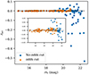 |
Fig. 1. Dependence of miniJPAS redshift errors on apparent magnitude. The ‘no odds cut’ sample (blue, squares) is obtained by imposing a redshift cut in MiniJPAS at zspec < 0.15, while the odds cut sample (orange, circles) has an additional cut in the odds value parameter (see text for details). The inset shows a zoom-in region centred on zero for a better visual inspection. |
Before applying the miniJPAS redshift errors to the IllustrisTNG galaxies, we first translated these redshift errors into distance errors, accounting for the IllustrisTNG snapshot being situated at z = 0.1. To do this, we added the miniJPAS redshift errors to the redshift of the IllustrisTNG snapshot (z0.1), as expressed in Eq. (2). The resulting perturbed redshifts (zpert) were then converted into corresponding perturbed luminosity distances (dpert)1. Finally, the distance errors (derr) were calculated by subtracting the perturbed distances (dpert) from the fixed luminosity distance at z = 0.1 (d = 475 Mpc).


Since Fig. 1 indicates that there is a substantial increase in the error amplitude beyond mr ≈ 19 (standard deviations of 0.002 for mr < 19 and 0.004 for mr > 19, respectively), we split the miniJPAS sample into two magnitude bins accordingly. We performed the same magnitude separation for IllustrisTNG galaxies by first computing their apparent magnitudes considering the snapshot redshift z0.1 and their absolute r magnitudes. We then randomly sampled derr, considering the two magnitude bins and added them to the Z-coordinate of galaxies2. The resulting standard deviation values for the distance errors are 7.1 Mpc for mr < 19 and 16.5 Mpc for mr > 19.
As a result, we obtained two galaxy mock samples: the ideal J-PAS (IllustrisTNG galaxies with mr < 21) and the perturbed J-PAS, where we additionally perturbed the coordinates, along one axis to mimic the miniJPAS redshift errors for such galaxies. In the upper panel of Fig. 3, we show plots of the ideal and perturbed galaxy mock samples in two different projections of the box. The smearing of galaxies due to the redshift errors is especially visible in the top right X − Z panel of the second plot.
We note that the redshift and odds cut that we impose on miniJPAS result in a very low number of galaxies (79), which we use to ascribe errors to a large number of galaxies (358 186). This approach may introduce artefacts in the galaxy distribution. We also tried the inverse transform sampling of the error distribution using both linear interpolation and the Gaussian approximation. The results from linear interpolation were quantitatively similar to the ones presented below, whereas the Gaussian approximation significantly overestimated the errors.
2.4. Watershed voids
Once we defined our galaxy mocks, we proceeded to the void identification with ZOnes Bordering On Voidness (ZOBOV Neyrinck 2008). For this task, we used VIDE (Sutter et al. 2014b), a frequently employed pipeline of the popular watershed transform method (Platen et al. 2007) used to detect voids in redshift surveys and N-body simulations. The pipeline is built on the ZOBOV algorithm, which computes the Voronoi tessellation of the tracer distribution to estimate the density field. The tessellation provides us with the minimum density values in our sample, the seeds of our voids. Subsequently, the watershed transform is applied in order to group the Voronoi cells together into voids. This allows us to reconstruct the void population and to preserve the shapes of voids (without any prior assumption of their geometry).
The pipeline internally computes various standard void properties. For example, it provides the void macrocentre defined as:
where xi and Vi represent the positions and Voronoi volumes of the galaxy tracers, respectively. VIDE also provides the equivalent radius of a void, defined as the radius of a sphere with the same volume as the void:
where V is the volume of the void, given by the sum of all the individual Voronoi cells. Furthermore, it offers easy access to the void member galaxies and allows one to study their properties and evolution. ZOBOV has been previously used in both observations (Fang et al. 2019; Hawken et al. 2020; Douglass et al. 2022) and simulations (Hamaus et al. 2015; Contarini et al. 2022; Kreisch et al. 2022); thus, it will allow for a fair comparison with existing results. Taken together, we considered this watershed-based method to be a suitable void identification method for our research goals of the J-PAS project.
We ran the VIDE pipeline on our J-PAS mock galaxy catalogue in order to obtain the void catalogues. We show an example of a detected void and its corresponding Voronoi cells in Fig. 2.
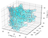 |
Fig. 2. Example of a void identified by ZOBOV. The void volume consists of Voronoi cells (red and cyan polygons) corresponding to its member galaxies (blue dots). The void contains 202 galaxies (and correspondingly consists of the same number of Voronoi cells) and encompasses a volume of about 2700 (Mpc/h)3. The minimum void density is |

Since ZOBOV is designed to find local minima in a density field and merge Voronoi cells until they form voids, some of the identified voids would actually be spurious. For example, it has already been shown that the ZOBOV algorithm manages to identify voids in a Poisson distribution (Neyrinck 2008). As a consequence, these spurious voids will present properties (e.g. densities) that would be in disagreement with the theoretical models of void formation (Sheth & van de Weygaert 2004; van de Weygaert & van Kampen 1993). Indeed, Nadathur & Hotchkiss (2014) have shown how ZOBOV can give rise to over-dense voids and cautioned that density criteria should be considered before using voids in cosmological tests.
Therefore, we needed to define specific criteria to clean the void catalogue of spurious detections. To establish these criteria, we first had to define some quantities. The void density, ρvoid, represents the ratio between the number of galaxies that define the void and the void volume. The minimum void density, ρmin, represents the lowest density of an associated Voronoi cell of a galaxy in a void. We note that this does not necessarily represent the density value at the void centre since voids usually do not contain matter there. Instead, this gives the density value associated with the largest volume of a Voronoi cell that comprises a void. We describe how we imposed criteria on these parameters in Sect. 3.
Furthermore, VIDE allows the user to merge voids and create a nested void hierarchy by modifying the initial density threshold parameter. This is an internal parameter of VIDE that is tweaked before the ZOBOV algorithm is applied to the galaxy distribution. This parameter essentially tells ZOBOV which initial voids should be merged together based on their density according to a threshold value. The parameter is initially set to a very low value, normalised to the average density (ρthreshold = 1 × 10⁻⁹), such that ZOBOV does not merge any voids; this is the value we used in our initial analysis. However, we can tweak this value and create a void hierarchy: zones with densities lower than the threshold are grouped together. A value of ρthreshold = 1 will essentially merge all the voids together into a single, parent super-void that spans the whole volume of the box and contains all the other children (sub-voids) grouped in different hierarchical levels. Intermediate values will give rise to various parent voids, potentially containing many children that occupy separate sub-volumes within the parent, separated by a ridge line. Voids that do not have any children are also a possibility. We discuss different merging thresholds used in this paper in Section 3.2.1.
To assess the voids in 3D space, for example, when calculating the overlap of voids between different data sets, we mapped the detected voids to a grid using the discrete Voronoi tesselation.
3. Results
In this paper, we address the questions of how J-PAS-like photometric redshift errors of galaxies affect the general properties of the identified void population (i.e., the number of detected voids, void radii, and void density profiles) and how well we can recover individual ‘true’ voids (identified from a galaxy mock dataset without redshift errors) from a dataset where we model redshift errors, as well as how well can we recover the overall void environment (e.g. at each volume element).
To answer these questions, we created two J-PAS galaxy mock datasets using the IllustrisTNG simulation: the ideal J-PAS sample, where we assumed no photometric redshift errors and the perturbed J-PAS sample, where we perturbed the Z-coordinate of galaxies with some distance errors corresponding to the actual errors occurring in miniJPAS, the precursor survey of J-PAS.
In this section, we present the results of the void identification obtained with the watershed ZOBOV algorithm. We show various properties of voids such as density parameters (Fig. 4), cumulative volume occupation distribution (Fig. 5), void abundance and radii (Fig. 6), and stacked radial density profiles (Fig. 7). We present comparisons between voids found in the ideal and perturbed samples based on various density- and radius-based filtering criteria, meant to increase the reliability of the detected voids (Table 1).
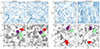 |
Fig. 3. Ideal and perturbed J-PAS galaxy mock samples (top panels) and void distributions (bottom panels) in X − Y and X − Z projections. We show a 10 Mpc-thick slice for each projection. The effect of redshift errors on the galaxy distribution is evident in the X − Z projection of the perturbed sample (fourth column, top panel). Cross-sections of voids are shown in greyscale, while colours highlight voids that have more than 50% volume overlap between the ideal and perturbed samples (see Sect. 3.2.1 for further discussion). A visual comparison reveals that voids detected in the ideal sample tend to fragment into various-sized voids in the perturbed sample. |
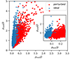 |
Fig. 4. Main plot: Void density parameters. The plot shows the correlation between the overall void density and the minimum void density for the unfiltered ideal (blue open circles) and perturbed samples (red squares). Inset: Same for medium-filtered voids. Both density parameters have been normalised to the average density in the box, |

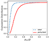 |
Fig. 5. Cumulative volume occupation distribution depending on ρmin for the unfiltered voids in the ideal and perturbed samples. |
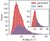 |
Fig. 6. Main plot: Void radius distributions for the unfiltered ideal and perturbed J-PAS mock samples. Inset: Same plot but for the medium-filtered voids. |
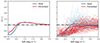 |
Fig. 7. Stacked radial number density profiles for the unfiltered (left) and filtered (right) ideal and perturbed sample voids. The horizontal line indicates the average number density of galaxies in the simulation box. The radii have been normalised to the average equivalent radii. For the filtered case, we also show the individual profiles of the 100 largest voids (thin lines, ideal sample – blue; perturbed sample – red). |
Properties of the voids before and after radius and density-based filtering.
One of the important tasks in our work is to recover voids in the ideal sample using the data from the perturbed sample. We looked at how well we can recover individual voids, setting 50% volume overlap as the threshold. Subsequently, we also studied how much of the overall void environment can be recovered (i.e. the total volume covered by voids in the two samples).
3.1. Void properties in J-PAS mocks
Using the ZOBOV algorithm, we identified 1065 voids in the ideal sample and 2558 voids in the perturbed sample of our mock J-PAS datasets. In Fig. 3, we show the galaxy distributions and the cross-sections of voids in a 10 Mpc-thick slice of the ideal and perturbed samples in two different projections of the box. The familiar elements of the cosmic web, such as filaments, superclusters, and voids, can be easily recognised in the X − Y projections of the ideal and perturbed samples. Due to the watershed transform retaining the topology of the field, we can immediately notice that voids are not isotropic structures and, instead, they come in a variety of shapes and sizes. We can also already see how the displacement of galaxies due to redshift errors impacts the galaxy distribution: a shift in the Z-direction moves galaxies in and out of the slice. Most notably, the underdense areas of the perturbed sample seem denser in the X − Y plane. It is possible to note (although less clearly) that structures such as clusters and filaments also become more diluted. As expected, the effect of redshift errors is especially visible in the X − Z projection (top right panel), where galaxies appear smeared across the figure vertically.
A visual inspection of the general population of voids (Fig. 3, bottom panels, shown in grey) in the ideal and perturbed samples confirms that there are more perturbed sample voids than ideal sample ones. This is most likely explained by voids in the ideal sample, which get fragmented into voids of various sizes in the perturbed sample (see also the right panel of Fig. 8). This comes as a direct consequence of the distance errors that shift the galaxy positions, which causes the ZOBOV algorithm to segment the galaxy population into different Voronoi cells that will group together into different voids. Thus, the void identification is highly sensitive to the precise position of galaxy tracers. Despite this fragmentation, we can see how some of the voids in the ideal and perturbed sample are still correlated (we show some of these voids with colours).
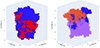 |
Fig. 8. Example of void volume overlaps between voids in the ideal and perturbed samples. Left: An ideal sample void (blue) overlapping with more than 50% with a perturbed sample void (red). Right: Different ideal sample void (blue, solid colour) overlapping with two perturbed sample voids, with different percentages (transparent colours). |
3.1.1. Void density parameters
It is natural to assume that voids are regions with densities generally below the Universe’s average density. However, the ZOBOV algorithm segments the whole galaxy population into voids; thus, spurious voids or voids within dense regions (e.g. superclusters), with average densities above the average of the Universe, should also be expected. We examined the situation by looking at the density parameters of the detected voids. Following the method of Nadathur & Hotchkiss (2014), we plot the correlation between the void density, ρvoid, and the minimum void density, ρmin, for the voids in the ideal and perturbed samples (Fig. 4). Both parameters were normalised in units of the average density over the simulation volume  .
.
We found that 631 voids (out of 1065, i.e. 59%) in the ideal and 1644 voids (out of 2558, i.e. 64%) in the perturbed samples have void densities larger than the average galaxy density. On average, both void samples present  . However, the voids in the ideal sample have a lower average minimum density (
 ) than the perturbed sample voids (
 ) indicating that their interior regions are emptier.
A commonly used definition of a void is based on the spherical model (see e.g. Bertschinger 1985; Sheth & van de Weygaert 2004), which states that a void is fully formed when it reaches an average density of  at the shell-crossing stage. Figure 4 shows that a substantial number of voids in our galaxy mocks have values that are even higher. This is again the result of ZOBOV dividing up the whole volume of the simulation box into voids and thus assigning over-dense filaments and walls to voids as their boundaries. This, in turn, raises the average density within voids. As such, obtaining voids by imposing a criterion on ρvoid in voids can lead to erroneous results. Instead, we decided to impose cuts based on the ρmin value. In this way, we were able to ensure that the starting seeds from which the algorithm builds up voids are under-dense and any spurious over-dense regions will thus be eliminated.
In addition to restricting the minimum void density, the total volume that voids occupy in the simulation box has to be taken into account as well. Previous work has shown that the void volume filling fraction in simulations ranges between 70%−90% (Ganeshaiah Veena et al. 2019; Hellwing et al. 2021; Curtis et al. 2024).
Taking these conditions into account, we defined three different levels of filtering for the voids in the ideal and perturbed samples: soft, medium, and strong. In Table 1, we give a summary of the way these filters were defined and the resultant void statistics. We focus on the medium level for the rest of the analysis of void properties and provide some comparisons with the soft- and strong-filtered void samples at the end.
To generate the medium-filtered void sample, we first imposed a density cut on the ρmin that eliminates all ideal sample voids with  . Imposing this criterion results in a ≈98% box volume coverage in voids. Additionally, to achieve a reasonable volume occupation percentage between ≈70%−90%, we also imposed a cut on the void radii; thus, we were able to eliminate all voids in the ideal sample with equivalent radii less than 12.5 Mpc h−1. Now voids in the ideal sample occupy 74% of the total Illustris volume and contain 331 voids.
In a similar way, we imposed a density cut on the perturbed sample voids, such that  (the reason for a slightly higher density threshold in the perturbed sample is that the remaining voids would only occupy ≈60% of the total volume in the box if we were to eliminate voids with
  ). This can be better understood by looking at Fig. 5, where we show the volume filling fraction as a function of ρmin. We can see how in the perturbed case, 60% of the volume is occupied by voids that have
  . We also removed all voids in the perturbed sample with a void radius of less than 5 Mpc h−1. We end up with a perturbed sample void population that occupies 77% of the simulation box volume and contains 951 voids.
We show a similar density parameter plot for the medium-filtered void samples in the inset of Fig. 4. For these void minimum density values, the correlation between the two parameters can no longer be observed. The average ρmin values are now  for voids in the ideal and
  for the ones in perturbed samples, respectively.
3.1.2. Void sizes
Next, we turned to the analysis of void sizes. As mentioned in Section 2, in the first approximation, the void size is defined by Eq. (6). In Fig. 6, we show the comparison of the void radius distributions between the ideal and perturbed samples considering both the unfiltered and medium-filtered voids. The unfiltered voids in the ideal dataset span a radii interval between 2.3 Mpc h−1 and 31.4 Mpc h−1 with an average radius of 10.7 Mpc h−1. On the other hand, the unfiltered voids in the perturbed dataset have radii between 1.6 Mpc h−1 and 25 Mpc h−1 with a mean radius of 8 Mpc h−1. The slightly smaller sizes of the voids in the perturbed sample agree well with Fig. 3, where we show how voids in the ideal sample get fragmented into voids in the perturbed sample, a direct consequence of the shift in the galaxy positions. If we impose the aforementioned radius and density cuts, the voids in the medium-filtered ideal sample span radii between 12.5 Mpc h−1 and 31.4 Mpc h−1 with an average of 16 Mpc h−1. In comparison, the medium-filtered perturbed voids have radii between 5.2 Mpc h−1 and 25 Mpc h−1, with a mean radius of 11 Mpc h−1.
3.1.3. Void density profiles
Another way to probe the voids for their matter content is by computing the stacked radial number density profile Δ(r) defined as:
where ρ(r) is the number density of galaxies in a spherical shell of thickness (r, r + dr), centred on the void macrocentre, and  is the average number density of galaxies in the simulation box.
We show the stacked radial profiles for the unfiltered ideal and perturbed sample voids in the left panel of Fig. 7. The radii have been normalised in each sample with the respective average void radius. Noise can be seen in the profiles – especially in the ideal case – due to the low number of voids and the simplicity of the spherical model. In both samples, we can see the familiar reverse spherical top-hat profile of a void. This is characterised by a mostly flat, under-dense interior that slowly rises above the average galaxy density, where the void ridge is located, and then it slowly decreases towards the mean density at larger distances (e.g. Sheth & van de Weygaert 2004). The over-dense boundaries in the density profiles arise due to the ZOBOV watershed method of identifying voids. In this approach, Voronoi cells are merged to form a void until the density of adjacent cells is lower than that of the merging cells. In other words, the merging process stops when a void ‘overflows’ into another, creating a high-density ridge that forms the void’s boundary and separates it from neighbouring voids.
In contrast, the perturbed sample voids present slightly higher densities in their centres than the ideal sample voids. This agrees well with the fact that perturbed sample voids have higher  and provide further confirmation that the redshift errors cause the ZOBOV algorithm to identify smaller and denser voids. On the other hand, the void ridges – or the peaks of the two unfiltered profiles – occur at around the same average density of ≈1.3ρ, with both slowly declining towards the average density in the box.
In the right panel of Fig. 7, we show the stacked density profiles for the medium-filtered sample, together with the 100 individual profiles for the largest voids in both ideal and perturbed samples. The radii have been normalised with respect to the average void radii of the filtered samples. As expected, the stacked profiles peak at lower density values than their unfiltered versions. Much as before, voids in the perturbed sample are slightly denser in their centres than their ideal sample counterparts. However, we can notice how the stacked void profile in the perturbed galaxy mock does not surpass the average density in the sample. Instead, it slowly increases and plateaus at the  . On the other hand, the voids in the ideal sample do retain a peak above the average density, albeit a less dense one.
A plausible explanation for the filtered perturbed profile is that the redshift errors blur out over-dense structures such as superclusters or filaments, thus reducing the density at the void boundary. This can be understood by looking at individual density profiles. We notice that filtered voids in the ideal sample have higher peaks in density in comparison with the voids in the perturbed sample. Thus, we consider why we do not see this effect in the unfiltered perturbed sample. Despite the redshift errors blurring out the over-dense structures at the void boundary, in doing so, they also raise (on average) the minimum density of a void (we can see this in Fig. 4). For a fixed ρvoid, the perturbed sample voids tend to have higher ρmin values in comparison with the ideal sample voids. Thus, by filtering perturbed voids by ρmin, we also tend to eliminate voids with higher values of ρvoid, which (in turn) will produce the stacked profile that we observe. This effect (or correlation) is less extreme in the ideal case.
An additional explanation may be offered by considering the structures in which voids themselves are embedded. The environment around voids can provide clues about their formation and evolution. Some voids are located within large overdensities (void-in-cloud) and will end up collapsing onto themselves over time. Others are embedded in larger underdensities (void-in-void) and tend to expand and merge into larger voids. In the void-in-void case, voids are surrounded by structures having densities less than or similar to the average background density. These voids tend to expand and remain under-dense. In the void-in-cloud case, the voids are surrounded by over-dense structures that will cause the voids to collapse and be ‘squeezed out of existence’ (Sheth & van de Weygaert 2004). These two different evolutionary pathways of voids can be understood via the density profiles. We suspect that the filtering criteria we imposed on the perturbed sample might eliminate the majority of voids embedded in over-dense regions and keep only the ones that are in the void-in-void scenario. This would make sense since we are keeping only the voids that are truly under-dense and these voids themselves might be surrounded by even larger underdensities. However, verifying this explanation will require further research.
3.2. Void recovery in J-PAS mocks
We have seen that the photometric redshift errors affect the galaxy distribution and, on average, give rise to a larger number of smaller and denser voids in the perturbed sample, thus affecting void identification and properties. The next step in our analysis was to recover as many individual ideal sample voids as possible from the perturbed sample, assuming that the latter is representative of what J-PAS would eventually observe.
To achieve this, we mapped the void volumes to a regular grid with 1 Mpc spacing using discrete Voronoi tessellation. We then compared the void volume overlap between the voids in the ideal and perturbed samples. In order to quantify the overlap, we considered two percentages: with respect to the ideal sample voids, Pi, and with respect to the perturbed sample voids, Pp:
where Vcom represents the common, overlapping volume between a void in the ideal sample and one in the perturbed sample, Vi is the volume of a void in the ideal sample, and Vp is the volume of a void in the perturbed sample. For a void in the perturbed sample to perfectly match a void in the ideal sample (or, in other words, to fully recover an ideal void), both Pi and Pp should be equal to 100%. For example, if Pi is equal to 100%, but the Pp has a different value, this means that the ideal void is wholly engulfed in the perturbed void; thus it does not represent the same void, but just a part of it.
3.2.1. Individual void recovery
To illustrate the individual void recovery, we show two scenarios of overlap in Fig. 8. The first scenario (left panel) shows an ideal sample void (blue) that has a 61% percentage overlap with a perturbed sample void (red); this means that despite the redshift errors moving galaxies around, we can recover more than half the volume of a specific void. While this is our desired scenario, the most common case (right panel) is that an ideal sample void (blue) is split into multiple voids in the perturbed sample due to the redshift errors.
We imposed a condition on both overlapping fractions to be higher than 50% and refer to these voids as ‘recovered voids’ throughout the remainder of the paper. Following this requirement, we managed to recover 53 voids, out of which 4 have more than 60% overlap; however, none exceed 70%. The volumes of these voids occupy around 6.6% of the box’s volume. In the filtered sub-samples, the number of recovered voids decreases to 43 (soft-filtered), 29 (medium-filtered), and 17 (strong-filtered).
In Fig. 9, we show the correlation between ρmin and void radius for unfiltered ideal and perturbed sample voids. Regardless of the sample, voids with larger radii are, in general, emptier of matter, which is in agreement with the void evolution theory (see e.g. Sheth & van de Weygaert 2004). As we have already seen, perturbed sample voids are, on average, slightly denser and smaller than those from the ideal sample. As such, the two distributions in Fig. 9 appear displaced from one another. We also show the recovered voids in ideal sample (yellow symbols) and their perturbed sample counterparts (cyan symbols). Their radii can be seen more clearly in the in-set histogram. In general, the two radii distributions tend to follow each other rather closely, as one would expect if the identified voids have similar volumes. Recovered ideal sample voids have radii spanning an interval between 6.5 Mpc h−1 and 23.3 Mpc h−1 with an average of 13.2 Mpc h−1, while the overlapping perturbed sample voids have radii in-between 6.3 Mpc h−1 and 20.7 Mpc h−1 with an average of 12.9 Mpc h−1. Looking at the average radius of the unfiltered voids in Table 1 suggests that the identification of larger voids is potentially less affected by redshift errors; thus, larger voids can be recovered with a higher degree of confidence than smaller ones.
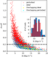 |
Fig. 9. Dependence of the minimum void density ρmin on the void radius R for the unfiltered ideal and perturbed sample voids. Larger voids tend to present lower matter content. We also show the recovered voids (53 in total) that present an overlap of more than 50% with yellow (for ideal) and cyan (for perturbed) symbols. The inset plot shows the radii for the recovered voids. The horizontal line defines the |

Another way we tried to increase the number of recovered voids is by merging voids based on a density threshold in the unfiltered perturbed sample (merging procedure was described in more detail in Section 2.4). The idea behind this method is that since the perturbed sample contains, on average, smaller voids, we could merge these voids into larger ones and potentially increase the void recovery. Overlapping void recovery with merging method works in the following way:
-
We choose a value for the merging threshold ρthreshold;
-
Obtain the new perturbed and merged void catalogue;
-
Compute the volume overlap percentages of the ideal voids and the perturbed merged voids to obtain the number of voids that have more than 50% overlap;
-
Filter the newly obtained catalogue via density and radius criteria cuts.
We tested this method for our unfiltered and medium-filtered perturbed samples by applying 4 different density merging thresholds (normalised to the average density): 0.1, 0.2, 0.3, and 0.4. Table 2 shows some statistics of the recovered voids for the two perturbed samples. In general, merging voids seems to have a positive effect, increasing the number of recovered voids, albeit by a small amount. However, not every threshold can increase this number. As can be seen, thresholds of 0.1 or lower will not merge enough voids to produce a visible difference in the recovery. On the other hand, past a certain threshold (> 0.2) the number of recovered voids slightly increases. The act of merging will produce large, supervoids that contain within themselves smaller voids. As we increase the merging threshold, the average radii (and the box volume occupied) of the voids increase and we end up with larger parent voids that can percolate; that is, they span the whole simulation volume. For this reason, coupled with the fact that merging voids and obtaining their volumes is computationally expensive, we do not go to thresholds higher than 0.4.
Statistics of unfiltered and medium-filtered perturbed and ideal voids that overlap more than 50% for different merging thresholds.
3.2.2. Void environment recovery
Another question we tackled regards the overall void environment comparison. We studied the total volume of all voids in both the ideal and perturbed samples. For example, for the un-filtered ideal and perturbed samples, the overlap of the total void environments is 100% since the watershed constructs voids in a way that divides up the whole simulation box exactly. The picture changes, however, once we impose the filtering criteria that would only maintain the more robust voids.
Similarly to the case with individual voids, we defined two environment overlapping fractions, Vcom/Vi and Vcom/Vp, except that now Vcom is the common overlapping volume of all the voids, while Vi and Vp are the total volumes covered by the voids in the ideal and perturbed samples, respectively. For medium-level filtering, we obtained values of approximately 80% for both overlaps. With respect to the simulation box volume, our common void environment occupies 61%. In comparing this with the individual void overlap, we may interpret it in the following way: the individual voids that VIDE identifies in the ideal and perturbed samples are different due to the redshift errors scrambling the spatial galaxy distribution and causing ideal sample voids to fragment into voids of various sizes in the perturbed sample. However, the overall void environment is similar.
To assess the significance of this result, we compared it to the probability that the overlap of the void volumes of the ideal and perturbed samples is occurring completely by chance. The simplest way is to shuffle the void grid cells for the perturbed galaxy sample, namely, randomise their positions. If the randomisation is uniform and independent, the resulting overlap of the void grid cells between the two samples depends only on the corresponding total volume fractions of voids. In this case, the overlap is the product of void volume fractions of both volumes Vi ⋅ Vp.
Using the void volume fractions from the Table 1, we obtained the following figures. For the medium-filtered voids, the common overlap volume fraction for the void environment in the data is 61% of the total volume of the box and 54% for the random sample. Similarly, for the soft and strong filters, the volume overlap fractions are 80% and 40%, while for the corresponding random samples, we get 77% and 31%, respectively. This implies that a harsher criterion will decrease the probability that the overlap occurs by chance.
4. Discussion and conclusions
Photometric redshift errors impact the observed spatial distribution of galaxies by inserting uncertainties along the line of sight. Consequently, this affects the scientific results and our understanding of the large-scale structure of the Universe.
In this paper, we modelled the expected redshift errors of the ongoing J-PAS photometric survey in order to understand their effect on the identification and properties of voids. To tackle this issue, we created mock galaxy catalogues of J-PAS using the IllustrisTNG N-body simulation and applied realistic redshift errors estimated from the smaller precursor miniJPAS survey. We aimed to recover voids detected from an ideal galaxy sample (without redshift errors) using a perturbed sample (with added redshift errors). We identified voids within these mocks using VIDE, a pipeline built on the ZOBOV watershed void identification algorithm and filtered voids using density-radius criteria to reduce the number of spurious ones. Our main results can be summarised as follows:
-
Photometric redshift errors do have a strong impact on void identification and properties. Voids in the ideal sample fragment into various-sized voids in the perturbed sample, which present, on average, denser interiors (0.36
 vs. 0.13
  ) and smaller sizes (8.00 Mpc h−1 vs. 10.70 Mpc h−1). These results can be seen in Figs. 6 and 7, respectively. Filtering out voids based on density and radius removes the spurious, smaller and denser voids in our data. Comparing the density profiles between the filtered ideal and perturbed sample voids reveals that, despite their denser interiors, voids in the perturbed sample have lower density boundaries (and lower average densities overall) in comparison with the voids in the ideal one (right panel of Fig. 7). This is a consequence of the errors blurring out surrounding over-dense structures, such as clusters and filaments, which define the void boundaries.
 -
Recovering individual voids is difficult. We assessed the individual void recovery in the ideal and perturbed samples by investigating the void volume overlap between these two samples. In the unfiltered samples, we identified 53 voids (out of the total of 1065 ideal sample voids) that overlap in volume by more than 50% (making up 6.6% of the total volume of the simulation box). If we consider a medium-level filtering, this number is reduced to 29 recovered voids (5.3% volume fraction). Merging perturbed voids by increasing the density threshold of VIDE slightly increased this number to 75 (14.9% void volume fraction) in the unfiltered sample and 50 (14.4%) in the medium-filtered sample. In general, merging voids has a positive effect on void recovery, albeit a small one. Furthermore, we find that larger voids are less affected by the redshift errors and, thus, more likely to be recovered then smaller voids (Fig. 9).
-
General void environment recovery is somewhat better than the recovery of individual voids. We also looked at the overall void environment overlap between the medium-filtered samples. This is defined as the total volume occupied by voids. We found that the environment overlaps with a percentage of 80% and occupies 61% volume of the simulation box for the medium-filtered voids. However, we note that given the large filling fraction of voids, even a random labelling would recover a significant fraction of the void grid cells, in our case, 54% of the simulation box volume. Increasing the strength of the filter does increase the difference in percentages, such that our strongest filtering will result in a 40% box volume occupation of the void environment overlap in the real samples and 31% in the random ones.
Curtis et al. (2024) investigated the properties of voids and void galaxies in the IllustrisTNG300-1 simulation using a spherical void-finding algorithm. They found 5078 voids at a snapshot of z = 0. Their smallest void has a radius of 2.5 Mpc h−1, comparable with the smallest void in our unfiltered ideal sample, while their largest void has a radius of 24.7 Mpc h−1. The median void radius found by the authors is 4.4 Mpc h−1. Overall, we found larger voids in both ideal and perturbed samples, which might be a consequence of the magnitude cuts that we imposed, essentially decreasing the number density of galaxies and thus increasing the average void radius (see e.g. Nadathur & Hotchkiss 2015; Paillas et al. 2017; Bermejo et al. 2024, for how tracer population impacts void properties). Furthermore, this may also be a consequence of the Voronoi tessellation used by the ZOBOV algorithm to identify voids. Since ZOBOV tessellates the whole galaxy distribution in the box, voids will end up having over-dense boundaries made out of filaments and walls. This, in turn, will make the volumes of the voids (and thus the equivalent radii) greater than the ones identified by a spherical void finder. The radius is also differently defined: VIDE defines the void radius as the radius of a sphere that has the same volume as the volume of a void (which, in turn, is defined as the sum of the volumes of the Voronoi cells). In contrast, the spherical void finder constructs spheres around void centres with radii such that the average void density is less than  . Their luminous density profile is also comparable to our unfiltered ideal sample, with an under-dense interior of
  . However, their profile does peak at a smaller radius since their voids are smaller on average. Another study by Dávila-Kurbán et al. (2023) also found void sizes between 7−11 Mpc h−1 when investigating galactic spins with respect to void centres in TNG300-1 simulation.
Regarding the individual void recovery, Sánchez et al. (2017) identified voids from a spectroscopic sample and from an equivalent photometric one by projecting galaxies into 2D slices and identifying voids within the 2D density field. These authors concluded that voids with sizes much larger than the photo-z error should not be affected by galaxy scattering. The median value of our photo-z error is ≈2 Mpc h−1, almost six times smaller than the average radii of the recovered voids. Interestingly, the authors mention that the structure on scales comparable to the photo-z errors will end up being erased. We tend to find that the smearing of galaxies will actually cause our ideal sample voids to end up being split into different perturbed sample voids, which, on average, present smaller radii. That said, the stacked density profile of the filtered perturbed sample voids does peak at a lower density than the ideal sample one (right panel of Fig. 7), suggesting that the over-dense structures, such as filaments and clusters bounding these voids, are smeared out.
There are some definite limitations of our work. Firstly, the number of miniJPAS galaxies used for estimating the photometric redshift errors is very small (79), especially in comparison with the number of galaxies in IllustrisTNG (358186). As more J-PAS data will be collected, this limitation can be overcome in future work. For example, a larger sample of observed galaxies might enable the selection of a sub-sample of sources with lower errors. Furthermore, J-PAS will provide additional information for void detection via weak-lensing analysis (Gruen et al. 2016; Peper et al. 2023). Secondly, the watershed ZOBOV algorithm proved not to be ideal for recovering voids based on volume overlap since it is extremely sensitive to galaxy tracers.
The recovered voids could potentially be used in studying the environmental effect that low-density regions have on the galaxy properties, while the overall void population statistics could be used in cosmological applications. Therefore, our future works will focus on improving the recovery of voids through different methods. For example, we might select only luminous red galaxies since they have lower photo-z errors or use clustering algorithms to trace galaxy groups instead of individual galaxies, thus averaging out the redshift uncertainties. Alternatively, a different void finder can be considered, such as one based on the Delaunay tessellation, since this would capture the density field more accurately via interpolation.
Astropy (Astropy Collaboration 2013, 2018, 2022).
Acknowledgments
We would like to thank the anonymous referee for the thorough report and useful comments which helped us to improve the manuscript. We acknowledge the support by the Estonian Ministry of Education and Research (grant TK202), Estonian Research Council grant (PRG2172, PRG1006, PSG700, PRG2159) and the European Union’s Horizon Europe research and innovation programme (EXCOSM, grant No. 101159513). This work is based on observations made with the JST/T250 telescope and JPCam at the Observatorio Astrofísico de Javalambre (OAJ), in Teruel, owned, managed, and operated by the Centro de Estudios de Física del Cosmos de Aragón (CEFCA). We acknowledge the OAJ Data Processing and Archiving Department (DPAD) for reducing and calibrating the OAJ data used in this work. Funding for the J-PAS Project has been provided by the Governments of Spain and Aragón through the Fondo de Inversión de Teruel, European FEDER funding and the Spanish Ministry of Science, Innovation and Universities, and by the Brazilian agencies FINEP, FAPESP, FAPERJ and by the National Observatory of Brazil with additional funding also provided by the University of Tartu and by the J-PAS Chinese Astronomical Consortium. VM thanks CNPq (Brazil) and FAPES (Brazil) for partial financial support. This paper has gone through an internal review by the J-PAS collaboration.
References
- Astropy Collaboration (Robitaille, T. P., et al.) 2013, A&A, 558, A33 [NASA ADS] [CrossRef] [EDP Sciences] [Google Scholar]
- Astropy Collaboration (Price-Whelan, A. M., et al.) 2018, AJ, 156, 123 [Google Scholar]
- Astropy Collaboration (Price-Whelan, A. M., et al.) 2022, ApJ, 935, 167 [NASA ADS] [CrossRef] [Google Scholar]
- Benitez, N., Dupke, R., Moles, M., et al. 2014, Highlights of Spanish Astrophysics VIII, 148 [Google Scholar]
- Bermejo, R., Wilding, G., van de Weygaert, R., et al. 2024, MNRAS, 529, 4325 [NASA ADS] [CrossRef] [Google Scholar]
- Bertschinger, E. 1985, ApJS, 58, 1 [NASA ADS] [CrossRef] [Google Scholar]
- Bertschinger, E. 1998, ARA&A, 36, 599 [Google Scholar]
- Beygu, B., Peletier, R. F., van der Hulst, J. M., et al. 2016, MNRAS, 464, 666 [Google Scholar]
- Blumenthal, G. R., da Costa, L. N., Goldwirth, D. S., Lecar, M., & Piran, T. 1992, ApJ, 388, 234 [NASA ADS] [CrossRef] [Google Scholar]
- Bond, J. R., Cole, S., Efstathiou, G., & Kaiser, N. 1991, ApJ, 379, 440 [NASA ADS] [CrossRef] [Google Scholar]
- Bonoli, S., Marín-Franch, A., Varela, J., et al. 2021, A&A, 653, A31 [NASA ADS] [CrossRef] [EDP Sciences] [Google Scholar]
- Boquien, M., Burgarella, D., Roehlly, Y., et al. 2019, A&A, 622, A103 [NASA ADS] [CrossRef] [EDP Sciences] [Google Scholar]
- Bromley, B. C., & Geller, M. J. 2024, ArXiv e-prints [arXiv:2407.03882] [Google Scholar]
- Buchert, T., Kerscher, M., & Sicka, C. 2000, Phys. Rev. D, 62, 043525 [Google Scholar]
- Carfora, M., & Familiari, F. 2024, ArXiv e-prints [arXiv:2401.04293] [Google Scholar]
- Clampitt, J., & Jain, B. 2015, MNRAS, 454, 3357 [NASA ADS] [CrossRef] [Google Scholar]
- Colberg, J. M., Sheth, R. K., Diaferio, A., Gao, L., & Yoshida, N. 2005, MNRAS, 360, 216 [NASA ADS] [CrossRef] [Google Scholar]
- Colberg, J. M., Pearce, F., Foster, C., et al. 2008, MNRAS, 387, 933 [NASA ADS] [CrossRef] [Google Scholar]
- Colless, M., Peterson, B. A., Jackson, C., et al. 2003, ArXiv e-prints [arXiv:astro-ph/0306581] [Google Scholar]
- Conrado, A. M., González Delgado, R. M., García-Benito, R., et al. 2024, A&A, 687, A98 [NASA ADS] [CrossRef] [EDP Sciences] [Google Scholar]
- Contarini, S., Verza, G., Pisani, A., et al. 2022, A&A, 667, A162 [NASA ADS] [CrossRef] [EDP Sciences] [Google Scholar]
- Contarini, S., Pisani, A., Hamaus, N., et al. 2024, A&A, 682, A20 [Google Scholar]
- Curtis, O., McDonough, B., & Brainerd, T. G. 2024, ApJ, 962, 58 [NASA ADS] [CrossRef] [Google Scholar]
- Dávila-Kurbán, F., Lares, M., & Lambas, D. G. 2023, MNRAS, 518, 3095 [Google Scholar]
- de Lapparent, V., Geller, M. J., & Huchra, J. P. 1986, ApJ, 302, L1 [Google Scholar]
- Douglass, K., Veyrat, D., Zaidouni, F., & BenZvi, S. 2022, Am. Astron. Soc. Meet. Abstr., 54, 139.23 [Google Scholar]
- Dressler, A. 1980, ApJ, 236, 351 [Google Scholar]
- Einasto, M., Deshev, B., Tenjes, P., et al. 2020, A&A, 641, A172 [NASA ADS] [CrossRef] [EDP Sciences] [Google Scholar]
- Einasto, M., Kipper, R., Tenjes, P., et al. 2021, A&A, 649, A51 [NASA ADS] [CrossRef] [EDP Sciences] [Google Scholar]
- Einasto, M., Kipper, R., Tenjes, P., et al. 2022, A&A, 668, A69 [NASA ADS] [CrossRef] [EDP Sciences] [Google Scholar]
- Fang, Y., Hamaus, N., Jain, B., et al. 2019, MNRAS, 490, 3573 [NASA ADS] [CrossRef] [Google Scholar]
- Ganeshaiah Veena, P., Cautun, M., Tempel, E., van de Weygaert, R., & Frenk, C. S. 2019, MNRAS, 487, 1607 [NASA ADS] [CrossRef] [Google Scholar]
- Genel, S., Vogelsberger, M., Springel, V., et al. 2014, MNRAS, 445, 175 [Google Scholar]
- González Delgado, R. M., Díaz-García, L. A., de Amorim, A., et al. 2021, A&A, 649, A79 [Google Scholar]
- Grogin, N. A., & Geller, M. J. 1999, AJ, 118, 2561 [NASA ADS] [CrossRef] [Google Scholar]
- Gruen, D., Friedrich, O., Amara, A., et al. 2016, MNRAS, 455, 3367 [Google Scholar]
- Hamaus, N., Sutter, P. M., Lavaux, G., & Wandelt, B. D. 2015, JCAP, 2015, 036 [Google Scholar]
- Hamaus, N., Pisani, A., Sutter, P., et al. 2016, Phys. Rev. Lett., 117, 091302 [NASA ADS] [CrossRef] [Google Scholar]
- Hawken, A. J., Aubert, M., Pisani, A., et al. 2020, JCAP, 2020, 012 [CrossRef] [Google Scholar]
- Hellwing, W. A., Cautun, M., van de Weygaert, R., & Jones, B. T. 2021, Phys. Rev. D, 103, 063517 [NASA ADS] [CrossRef] [Google Scholar]
- Hernán-Caballero, A., Varela, J., López-Sanjuan, C., et al. 2021, A&A, 654, A101 [NASA ADS] [CrossRef] [EDP Sciences] [Google Scholar]
- Hernán-Caballero, A., Akhlaghi, M., López-Sanjuan, C., et al. 2024, A&A, 684, A61 [NASA ADS] [CrossRef] [EDP Sciences] [Google Scholar]
- Hoffman, Y., & Shaham, J. 1982, ApJ, 262, L23 [NASA ADS] [CrossRef] [Google Scholar]
- Hoyle, F., & Vogeley, M. S. 2002, ApJ, 566, 641 [NASA ADS] [CrossRef] [Google Scholar]
- Hoyle, F., & Vogeley, M. S. 2004, ApJ, 607, 751 [NASA ADS] [CrossRef] [Google Scholar]
- Hoyle, F., Vogeley, M. S., & Pan, D. 2012, MNRAS, 426, 3041 [NASA ADS] [CrossRef] [Google Scholar]
- Icke, V. 1984, MNRAS, 206, 1P [NASA ADS] [CrossRef] [Google Scholar]
- Jõeveer, M., Einasto, J., & Tago, E. 1978, MNRAS, 185, 357 [Google Scholar]
- Jaber, M., Peper, M., Hellwing, W. A., Aragón-Calvo, M. A., & Valenzuela, O. 2024, MNRAS, 527, 4087 [Google Scholar]
- Jennings, E., Li, Y., & Hu, W. 2013, MNRAS, 434, 2167 [CrossRef] [Google Scholar]
- Kirshner, R. P., Oemler, A., Schechter, P. L., & Shectman, S. A. 1987, ApJ, 314, 493 [NASA ADS] [CrossRef] [Google Scholar]
- Kitaura, F.-S., Chuang, C.-H., Liang, Y., et al. 2016, Phys. Rev. Lett., 116, 171301 [NASA ADS] [CrossRef] [Google Scholar]
- Kreckel, K., Platen, E., Aragón-Calvo, M. A., et al. 2012, AJ, 144, 16 [Google Scholar]
- Kreisch, C. D., Pisani, A., Carbone, C., et al. 2019, MNRAS, 488, 4413 [NASA ADS] [CrossRef] [Google Scholar]
- Kreisch, C. D., Pisani, A., Villaescusa-Navarro, F., et al. 2022, ApJ, 935, 100 [NASA ADS] [CrossRef] [Google Scholar]
- Lacey, C., & Cole, S. 1993, MNRAS, 262, 627 [NASA ADS] [CrossRef] [Google Scholar]
- Laur, J., Tempel, E., Tamm, A., et al. 2022, A&A, 668, A8 [NASA ADS] [CrossRef] [EDP Sciences] [Google Scholar]
- Lavaux, G., & Wandelt, B. D. 2010, MNRAS, 403, 1392 [NASA ADS] [CrossRef] [Google Scholar]
- Liddle, A. R., & Lyth, D. H. 1993, Phys. Rep., 231, 1 [Google Scholar]
- Marinacci, F., Vogelsberger, M., Pakmor, R., et al. 2018, MNRAS, 480, 5113 [NASA ADS] [Google Scholar]
- Maturi, M., Finoguenov, A., Lopes, P. A. A., et al. 2023, A&A, 678, A145 [NASA ADS] [CrossRef] [EDP Sciences] [Google Scholar]
- Nadathur, S., & Hotchkiss, S. 2014, MNRAS, 440, 1248 [NASA ADS] [CrossRef] [Google Scholar]
- Nadathur, S., & Hotchkiss, S. 2015, MNRAS, 454, 889 [NASA ADS] [CrossRef] [Google Scholar]
- Naiman, J. P., Pillepich, A., Springel, V., et al. 2018, MNRAS, 477, 1206 [Google Scholar]
- Nelson, D., Pillepich, A., Springel, V., et al. 2018, MNRAS, 475, 624 [Google Scholar]
- Neyrinck, M. C. 2008, MNRAS, 386, 2101 [CrossRef] [Google Scholar]
- Padilla, N. D., Ceccarelli, L., & Lambas, D. G. 2005, MNRAS, 363, 977 [Google Scholar]
- Paillas, E., Lagos, C. D. P., Padilla, N., et al. 2017, MNRAS, 470, 4434 [NASA ADS] [CrossRef] [Google Scholar]
- Pan, D. C., Vogeley, M. S., Hoyle, F., Choi, Y.-Y., & Park, C. 2012, MNRAS, 421, 926 [NASA ADS] [CrossRef] [Google Scholar]
- Peper, M., & Roukema, B. F. 2021, MNRAS, 505, 1223 [NASA ADS] [CrossRef] [Google Scholar]
- Peper, M., Roukema, B. F., & Bolejko, K. 2023, MNRAS, 525, 91 [NASA ADS] [CrossRef] [Google Scholar]
- Pillepich, A., Nelson, D., Hernquist, L., et al. 2018, MNRAS, 475, 648 [Google Scholar]
- Pisani, A., Massara, E., Spergel, D. N., et al. 2019, BAAS, 51, 40 [Google Scholar]
- Planck Collaboration XIII. 2016, A&A, 594, A13 [NASA ADS] [CrossRef] [EDP Sciences] [Google Scholar]
- Platen, E., van de Weygaert, R., & Jones, B. J. T. 2007, MNRAS, 380, 551 [NASA ADS] [CrossRef] [Google Scholar]
- Press, W. H., & Schechter, P. 1974, ApJ, 187, 425 [Google Scholar]
- Räsänen, S. 2004, JCAP, 2004, 003 [CrossRef] [Google Scholar]
- Rosas-Guevara, Y., Tissera, P., Lagos, C. D. P., Paillas, E., & Padilla, N. 2022, MNRAS, 517, 712 [NASA ADS] [CrossRef] [Google Scholar]
- Roukema, B. F. 2018, A&A, 610, A51 [NASA ADS] [CrossRef] [EDP Sciences] [Google Scholar]
- Sánchez, C., Clampitt, J., Kovacs, A., et al. 2017, MNRAS, 465, 746 [CrossRef] [Google Scholar]
- Schuster, N., Hamaus, N., Pisani, A., et al. 2019, JCAP, 2019, 055 [Google Scholar]
- Sheth, R. K., & van de Weygaert, R. 2004, MNRAS, 350, 517 [NASA ADS] [CrossRef] [Google Scholar]
- Springel, V., Pakmor, R., Pillepich, A., et al. 2018, MNRAS, 475, 676 [Google Scholar]
- Sutter, P. M., Pisani, A., Wandelt, B. D., & Weinberg, D. H. 2014a, MNRAS, 443, 2983 [NASA ADS] [CrossRef] [Google Scholar]
- Sutter, P. M., Lavaux, G., Hamaus, N., et al. 2014b, Astrophysics Source Code Library [record ascl:1407.014] [Google Scholar]
- Tamone, A., Zhao, C., Forero-Sánchez, D., et al. 2023, MNRAS, 526, 2889 [NASA ADS] [CrossRef] [Google Scholar]
- Tempel, E., & Tamm, A. 2015, A&A, 576, L5 [NASA ADS] [CrossRef] [EDP Sciences] [Google Scholar]
- van de Weygaert, R., & van Kampen, E. 1993, MNRAS, 263, 481 [NASA ADS] [Google Scholar]
- Verweg, D. B. H., Jones, B. J. T., & van de Weygaert, R. 2023, arXiv e-prints [arXiv:2310.19451] [Google Scholar]
All Tables
Statistics of unfiltered and medium-filtered perturbed and ideal voids that overlap more than 50% for different merging thresholds.
All Figures
|
Fig. 1. Dependence of miniJPAS redshift errors on apparent magnitude. The ‘no odds cut’ sample (blue, squares) is obtained by imposing a redshift cut in MiniJPAS at zspec < 0.15, while the odds cut sample (orange, circles) has an additional cut in the odds value parameter (see text for details). The inset shows a zoom-in region centred on zero for a better visual inspection. |
| In the text | |
|
Fig. 2. Example of a void identified by ZOBOV. The void volume consists of Voronoi cells (red and cyan polygons) corresponding to its member galaxies (blue dots). The void contains 202 galaxies (and correspondingly consists of the same number of Voronoi cells) and encompasses a volume of about 2700 (Mpc/h)3. The minimum void density is |
| In the text | |
|
Fig. 3. Ideal and perturbed J-PAS galaxy mock samples (top panels) and void distributions (bottom panels) in X − Y and X − Z projections. We show a 10 Mpc-thick slice for each projection. The effect of redshift errors on the galaxy distribution is evident in the X − Z projection of the perturbed sample (fourth column, top panel). Cross-sections of voids are shown in greyscale, while colours highlight voids that have more than 50% volume overlap between the ideal and perturbed samples (see Sect. 3.2.1 for further discussion). A visual comparison reveals that voids detected in the ideal sample tend to fragment into various-sized voids in the perturbed sample. |
| In the text | |
|
Fig. 4. Main plot: Void density parameters. The plot shows the correlation between the overall void density and the minimum void density for the unfiltered ideal (blue open circles) and perturbed samples (red squares). Inset: Same for medium-filtered voids. Both density parameters have been normalised to the average density in the box, |
| In the text | |
|
Fig. 5. Cumulative volume occupation distribution depending on ρmin for the unfiltered voids in the ideal and perturbed samples. |
| In the text | |
|
Fig. 6. Main plot: Void radius distributions for the unfiltered ideal and perturbed J-PAS mock samples. Inset: Same plot but for the medium-filtered voids. |
| In the text | |
|
Fig. 7. Stacked radial number density profiles for the unfiltered (left) and filtered (right) ideal and perturbed sample voids. The horizontal line indicates the average number density of galaxies in the simulation box. The radii have been normalised to the average equivalent radii. For the filtered case, we also show the individual profiles of the 100 largest voids (thin lines, ideal sample – blue; perturbed sample – red). |
| In the text | |
|
Fig. 8. Example of void volume overlaps between voids in the ideal and perturbed samples. Left: An ideal sample void (blue) overlapping with more than 50% with a perturbed sample void (red). Right: Different ideal sample void (blue, solid colour) overlapping with two perturbed sample voids, with different percentages (transparent colours). |
| In the text | |
|
Fig. 9. Dependence of the minimum void density ρmin on the void radius R for the unfiltered ideal and perturbed sample voids. Larger voids tend to present lower matter content. We also show the recovered voids (53 in total) that present an overlap of more than 50% with yellow (for ideal) and cyan (for perturbed) symbols. The inset plot shows the radii for the recovered voids. The horizontal line defines the |
| In the text | |
Current usage metrics show cumulative count of Article Views (full-text article views including HTML views, PDF and ePub downloads, according to the available data) and Abstracts Views on Vision4Press platform.
Data correspond to usage on the plateform after 2015. The current usage metrics is available 48-96 hours after online publication and is updated daily on week days.
Initial download of the metrics may take a while.