| Issue |
A&A
Volume 695, March 2025
|
|
|---|---|---|
| Article Number | A28 | |
| Number of page(s) | 10 | |
| Section | Astronomical instrumentation | |
| DOI | https://doi.org/10.1051/0004-6361/202452671 | |
| Published online | 28 February 2025 | |
Polarization aberrations in next-generation Giant Segmented Mirror Telescopes (GSMTs)
II. Influence of segment-to-segment coating variations on high-contrast imaging and polarimetry
1
Steward Observatory, University of Arizona,
933N Cherry Avenue,
Tucson,
AZ
85721,
USA
2
James C. Wyant College of Optical Sciences, University of Arizona,
933N Cherry Avenue,
Tucson,
AZ
85721,
USA
3
Department of Physics, University of California,
Santa Barbara,
CA
93106,
USA
4
Leiden University,
Niels Bohrweg 2,
2333 CA
Leiden,
The Netherlands
5
European Southern Observatory (ESO),
Alonso de Córdova 3107, Vitacura, Casilla 19001,
Santiago de Chile,
Chile
6
TMT International Observatory LLC,
100 W. Walnut St., Suite 300,
Pasadena,
CA
91124,
USA
★★ Corresponding author; This email address is being protected from spambots. You need JavaScript enabled to view it.
Received:
18
October
2024
Accepted:
6
January
2025
Abstract
Context. Direct exo-earth imaging is a key science goal for astronomy in the next decade. This ambitious task imposes a target contrast of ≈10−7 at wavelengths from I to J-band. In our prior study, we determined that polarization aberrations can limit the achievable contrast to 10−5 to 10−6 in the infrared. However, these results assumed a perfect coronagraph coupled to a telescope with an ideal coating on each of the mirrors.
Aims. In this study we seek to understand the influence of polarization aberrations from segment-to-segment coating variations on coronagraphy and polarimetry.
Methods. We use the Poke open-source polarization ray tracing package to compute the Jones pupil of each GSMT with spatially- varying coatings applied to the segments. The influence of the resultant polarization aberrations is simulated by propagating the Jones pupil through physical optics models of coronagraphs using HCIPy.
Results. After applying wavefront control from an ideal adaptive optics system, we determine that the segment-to-segment variations applied limit the performance of coronagraphy to a raw contrast of approximately 10−8 in I-band, which is 2–3 orders of magnitude lower the target performance for high-contrast imaging systems on the ground. This is a negligible addition to the nominal polarization aberrations for ground-based systems. We further observe negligible degradation in polarimetric imaging of debris disks from segment-to-segment aberrations above and beyond the impact of nominal polarization aberration.
Key words: polarization / instrumentation: adaptive optics / instrumentation: high angular resolution / instrumentation: polarimeters
NASA Hubble Fellow.
© The Authors 2025
 Open Access article, published by EDP Sciences, under the terms of the Creative Commons Attribution License (https://creativecommons.org/licenses/by/4.0), which permits unrestricted use, distribution, and reproduction in any medium, provided the original work is properly cited.
This article is published in open access under the Subscribe to Open model. This email address is being protected from spambots. You need JavaScript enabled to view it. to support open access publication.
1 Introduction
The next generation Giant Segmented Mirror Telescopes (GSMT’s, shown in Figure 1) will be the premier astronomical tools on the ground for direct imaging of faint exoplanets. The high angular resolution imaging enabled by their >25m apertures has the potential to expand the discovery space of exoplanets to include Earth-like planets. To fit in a reasonable volume, these large observatories employ fast primary mirrors (≈F/1) and fold mirrors with high angles of incidence (≈30°–45°), which result in polarization aberrations that can limit coronagraphy.
Polarization aberrations typically manifest as low-order aberrations (e.g., tilt, astigmatism) whose magnitude depends on the polarization state of the incoming light. Diattenuation is the aberration of the amplitude as a function of polarization, while retardance is the aberration of phase as a function of polarization (Chipman et al. 2018; Breckinridge et al. 2018). These can combine to result in aberrations of opposite sign for orthogonal polarization states. A formalism for polarization aberration was first introduced to astronomy in Sanchez Almeida & Martinez Pillet (1992). To understand the polarization aberrations manifesting as beam shifts in astronomical telescopes, van Holstein et al. (2023) describes the polarization aberrations for an inclined flat mirror in terms of Goos–Hänchen and Imbert–Federov beam shifts and discusses their implication on the coronagraphic performance.
Although high-contrast imaging instruments employ extreme wavefront sensing and control, the adaptive optics (AO) system cannot simultaneously correct for aberrations in orthogonal polarization states (Breckinridge et al. 2015). Polarization aberrations are purely a function of the angle of incidence (AOI) and the coating on the optical surface. For a single layer, the diattenuation and retardance scale roughly quadratically with the AOI. However, most observatory mirrors are coated with a dielectric layer to enhance reflectivity or prevent oxidation of the primary reflecting layer, which can increase the retardance and degrade the coronagraphic performance.
The effect of polarization aberrations is far from new and has been observed in some of the current high- contrast imaging instruments in ground-based observatories. The SPHERE/ZIMPOL polarimetric imager has observed a shift between orthogonal polarization states that results in residual noise in the polarization differential imaging measurements as shown in Schmid et al. (2018). Subaru Telescope’s SCExAO instrument and the SPHERE/IRIDIS instrument both requires substantive calibration of instrumental polarization to perform accurate polarimetry (Hart et al. 2021; Zhang et al. 2023; van Holstein et al. 2020). The Gemini Planet Imager has shown that a differential astigmatism term between orthogonal polarization states is visible in polarized observations (Millar-Blanchaer et al. 2022b). These aberrations were incorporated during the design considerations of high-contrast imaging systems for next-generation space-based telescopes. For example, the design of the proposed HabEx (Gaudi et al. 2020) and LUVOIR (Will & Fienup 2019) missions was driven partly to minimize the polarization aberrations that degrade the coronagraphic performance. Balasubramanian et al. (2005) developed optimized mirror coatings to reduce the polarization aberrations for the proposed Terrestrial Planet Finder Coronagraph (TPF-C). Further, Luo et al. (2020) simulated the polarization aberrations for a 2 m, F/14 three-mirror anastigmat (TMA) telescope to estimate the PSF ellipticity affecting the measurements of weak gravitational lensing. Anche et al. (2023a); Doelman et al. (2023) have performed simulations of high-contrast polarimetric observations of disks and planets for the upcoming Nancy Grace Roman Coronagraph instrument (Kasdin et al. 2020) to show that polarization aberration residuals are below the expected coronagraphic performance.
For the proposed future Habitable Worlds Observatory (HWO) aiming to achieve a raw contrast of 10–10, minimizing the polarization aberrations is expected to be one of the driving requirements. As a preliminary analysis for the HWO, Anche et al. (2023b) modeled polarization aberrations for 6m on-axis and off-axis TMA designs using different coating recipes for the mirrors and demonstrated that the coating recipe (refractive index and thickness of the protective coating) plays a vital role in the polarization aberrated coronagraphic performance. Thus, modeling polarization aberrations and estimating their effect on the contrast is critical for next-generation telescopes with high-contrast imaging instruments.
The first paper in this series on polarization aberrations in GSMTs, Anche et al. (2023), demonstrated the effect of polarization aberrations on coronagraphic performance by presenting simulations of a static polarization model of the telescope with perfect coronagraphs (PC). We refer the reader to Anche et al. (2023) for a complete description of the simulations. Below, we summarize only the model parameters and important findings of the study.
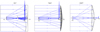 |
Fig. 1 Optical layout of the telescopes from Zemax® for the three GSMT’s. The TMT and ELT are cassegrain-type telescopes with a fold mirror configuration, whereas the GMT is Gregorian-type telescope with a fold mirror. |
2 Review of previous findings
We model and perform the raytracing of the GSMTs using Zemax® and obtain Jones pupils using the Python-based polarization ray tracing package (PRT), Poke (Ashcraft et al. 2023). The TMT and ELT mirror coating were a four-layer Gemini-like coating (Schneider et al. 2016), and bare Aluminum was used on GMT. We simulated the Jones Pupils at the exit pupil for each of the telescopes using PRT for astronomical filter bands U to N. The eigenvalues of the Jones pupils were used to estimate diattenuation and retardance. Among the three GSMTs, GMT showed the highest diattenuation, followed by TMT and ELT, while TMT showed the highest retardance, followed by ELT and GMT. The retardance of all three telescopes reduces with increasing wavelength. On the other hand, diattenuation for GMT showed an increasing trend in optical and near-IR wavelength regimes due to the refractive index variation of bare aluminum. The high retardance for TMT and ELT is attributed to the 4-layer Gemini-like coating.
The wavefront sensing and control system can compensate for the common aberrations between the X and Y polarized light. Thus, they are removed from the Jones pupils ϕxx and ϕyy terms (see Figure 5 in Anche et al. 2023) and propagated through the perfect coronagraphs that remove the electric field modes based on their spatial order (2, 4, and 6; Cavarroc et al. 2006; Guyon et al. 2006). The achievable peak raw contrast for all three telescopes is limited by the dominant polarization aberrations: retardance tilt (i.e. beam shifts), and retardance defocus (i.e. differential astigmatism). For a brief introduction to these aberrations, please refer to Section 1 of Anche et al. (2023). As these polarization aberrations depend on the refractive index variation, the chromatic behavior is seen in the residual images for each telescope over the different filter bands.
The peak raw contrast is calculated using the coronagraphic residual images for each of the telescopes at each filter band. The high-contrast imaging instruments onboard the GSMTs are expected to obtain a peak contrast of 10–5–10–6 in the R and I-bands to search for biomarkers such as oxygen A-band at 720nm (Kasper et al. 2021; Males et al. 2022). However, simulations in Anche et al. (2023) show that the peak raw contrast is >10–5 for all the three GSMTs in the U–y bands for the 2nd and 4th order coronagraphs, which is an order of magnitude worse than the required performance. The peak raw contrast in the order of 10–5–10–6 is obtained only for the J–N bands.
Among all three GSMTs, the ELT shows the worst contrast degradation due to polarization aberrations because it has five mirrors coated with a 4-layer coating and the fastest primary (F/0.7) compared to TMT (F/1). Although GMT also has a fast primary (F/0.87), it outperforms the TMT and ELT by an order of magnitude as its mirrors are coated with bare aluminum and therefore have the lowest retardance. Models in which the GMT mirrors are coated with bare silver and Gemini-like coating yield a peak raw contrast performance of GMT that is very similar to that of ELT and TMT. Thus, coating plays a significant role in the magnitude of the polarization aberrations, and optimized coating recipes would reduce the aberrations (van Holstein et al. 2023). The previous modeling and simulations were performed using an ideal coating recipe on all the telescope mirrors, including primary mirror segments for all three GSMTs. Additionally, for GMT mirrors coated with bare aluminum, the influence of Al2O3 on bare aluminum was not considered, which has been observed before in aluminum-coated telescope mirrors (van Harten et al. 2009; Sankarasubramanian et al. 1999).
In this study, we aim to bring these findings to the next level of fidelity by examining how segment-to-segment coating variations will influence high-contrast imaging and polarimetry. In Section 3, we develop the modeling of the GSMTs subject to segment-to-segment variations using integrated PRT and diffraction models. In Section 4, we use these models to re-evaluate the coronagraphic performance of the GSMTs subject to these effects by statistically probing the possible space of segment- to-segment variations. In Section 5, we use these models to understand how polarization aberrations influence polarimetric imaging of distant point sources and debris disks. We summarize our findings and provide recommendations in Section 6.
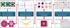 |
Fig. 2 Steps to simulate polarimetric imaging of a generally off-axis source in the presence of polarization aberrations through the GSMTs is described here. As a first step, we simulate the segment-to-segment coating variation to be a sum of the piston, tilt, and focus terms of the Zernike polynomials. We then perform the PRT using Poke to estimate Jones pupils for all three telescopes. The Jones pupils and the corresponding low- order polarization aberration terms that are fit to these Jones pupils are available in Anche et al. (2023b). The Jones pupils are propagated through the perfect coronagraphs to calculate the residuals and the peak raw contrast. The Jones pupils are further used to estimate the Amplitude Response Matrix and Mueller Point Response Matrix for use in extended scene simulation. |
3 Modeling approach
In this work we simulate the influence of coating variations on polarization aberrations with PRT. PRT is a method of propagating the complex amplitudes of orthogonal polarization states through three dimensional optical systems. We review this technique in Section 3 of our previous work (Anche et al. 2023). This review is not exhaustive for readers that may be interested in reproducing the PRT algorithm, so we also refer readers to Chapters 10 and 11 of Chipman et al. (2018). To perform PRT we use the Python package Poke: an open-source ray-based physical optics platform (described in Ashcraft et al. 2023). In our previous study we built PRT into Poke to compute the Jones pupil of the GSMTs. Poke directly interfaces with other open-source physical optics packages like High Contrast Imaging in Python (HCIPy, Por et al. 2018), which we use to simulate the diffraction response of a coronagraph to polarization aberrations. Poke can perform PRT with arbitrary thin-film multilayer stacks with spatial variation, which will be key in simulating spatially-varying coating thicknesses on the GSMTs. The code used to conduct the simulations in this study can be found at Ashcraft (2024), and we illustrate its operation in Figure 2.
Understanding what shape the coating thickness variation will take is somewhat difficult because of the challenge of measuring coating thicknesses across meter-scale segments. However, we can begin to understand the spatial distribution of a given coating by looking to work conducted by Gemini Observatory. The Gemini primary mirror coating chamber uses magnetron sputtering to deposit their protected silver coating. Magnetron sputtering operates by applying an electrical bias on the material to deposit (called the “target,” e.g. aluminum, silver). The bias attracts the plasma, resulting in high-energy collisions that free matter from the target and allow it to fly toward the substrate being coated. The deposition rate of this coating process is high, but difficult to conduct with spatial uniformity on large optics. Investigators at Gemini telescope studied witness samples from their coating chamber ellipsometrically to determine the coating thickness deposited across a substrate, and found a 15% (or 1.3 nm) peak-to-valley variation in the deposited coating over a 4 cm × 4 cm substrate (Schneider et al. 2016). When considering the geometry of typical coating chambers, we know that the predominant modes of nonuniform coating deposition appear as a mixture of tilt and focus-like shapes (Bishop et al. 2019). Furthermore, the TMT is considering a similar coating recipe and procedure, and expects variations in the coating thickness as large as 10–20% (Skidmore et al. 2023, Private Communication).
To model these effects, we consider the dielectric coating on each mirror segment to be a sum of the piston, tilt, and focus terms of the Zernike polynomials. These thickness variations are applied to the overcoat layer of the ELT and TMT (illustrated in Figure 3). The coating thickness variation on the underlying reflective layer for the GSMTs will predominantly manifest as a wavefront aberration that is common to all polarization states, which will be removed by the AO system. Therefore, we assume an ideally deposited reflective layer. The GMT will not have a dielectric overcoat layer, but van Harten et al. (2009) showed that the aluminum oxide layer that grows on bare aluminum substrates could result in negative consequences to polarimetry. The spatial distribution of this growth is unknown, so we elect to simulate it with a power law whose power spectral density (PS D) is defined by the power law in Equation (1)1,
 (1)
(1)
where r is the radial spatial frequency and n is the power law index. van Harten et al. (2009) suggests that the Al2O3 layer approaches a thickness of 4.12 ± 0.08nm roughly 800 hours after being coated, but the result is computed from an ellipsometer which spatially averages the coating. Therefore we will assign the power law distribution with a peak-to-valley equal to the uncertainty in the measurement. One such resulting surface from this approach is shown in Figure 4. The power law index n is also not well-understood for telescope primary mirrors, so we simulate several cases in this study to parameterize the influence of this quantity. Given the uncertainty in the dielectric layer for the TMT and ELT, we also consider two cases where the film peak- to-valley film variation is 20% and 50%. Table 1 summarizes the thickness variation we simulate for each of the GSMTs. Note that we hold the GMT peak-to-valley variation the same, but instead vary the power law index n.
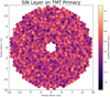 |
Fig. 3 Example of low-order coating variation on the TMT primary mirror. We generate a random set of Zernike coefficients from Z1–Z4 and apply it to each segment using the prysm numerical optics package. The error is normalized to have a peak-to-valley of 10% of the nominal thickness and then added to the nominal thickness. Quantifying the impact of these errors on coronagraphy and polarimetry is important to understanding the as-built performance of the GSMTs. |
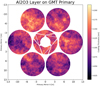 |
Fig. 4 Example of the PSD-generated coating variation assigned on the GMT primary mirror. We generate a power law with a given index n and then enforce its peak-to-valley variation to be consistent with the ±0.08 nm from van Harten et al. (2009). Varying the PSD index n allows us to parameterize the influence of the aluminum oxide layer on the GMT. |
Parameters for spatial variations used for each case studied for each GSMT.
4 Effect on coronagraphy
Since the coronagraph architectures for the GSMTs are not finalized, we repeat the procedure from our previous study and employ the Perfect Coronagraph (PC) models described in Guyon et al. (2006) and Cavarroc et al. (2006). These are readily accessible with polarized field propagation in HCIPy and described in Section 6 of Anche et al. (2023).
We statistically sample the random realizations of the thickness variations specified by Table 1 using a set of 25 randomized trials for each Case, GSMT, and PC order (2, 4, 6). An example of one such set of trials is shown in Figure 5, where we simulate Case 2 for the ELT equipped with a 2nd-order PC. We then subtract off the coronagraphic image assuming a perfectly uniform coating to arrive at the change in contrast introduced by the spatially-varying coating. The change in contrast is observed to be small (maximizes near 1λ/D at ≈10–8), and the plot of the RMS roughly envelopes the individual trials. For another example in 2D, we show the log-scaled difference of one realization of these PSFs for the GMT with the nominal polarization aberrated PSF subtracted in Figure 7. This Figure shows the influence of increasing power law index n, as well as the structure of the residual aberration.
In Figure 6, we show the RMS of the Case 2 trials for all GSMTs and coronagraph orders. These data represent the expected variability in contrast that is created by applying spatially non-uniform errors across each mirror segment, and correcting the resulting scalar wavefront error with the AO system. We observe that order 2 and 4 coronagraphs behave very similarly and that the order 6 coronagraph performs orders of magnitude better, which is consistent with our results in Anche et al. (2023). For Case 2, the expected variability peaks with the TMT at 1.7 × 10⁻⁸ contrast. To put this in context, the signal from the segment-to-segment errors is 100 times fainter than the AO residuals projected for high-contrast imaging instruments on these systems. This is a very encouraging result, because it suggests that nonuniform coatings on the primary mirrors of the GSMTs will not be a limiting factor in high-contrast imaging. The same Figures for Case 1 and 3 can be found in Appendix A, but the worst case scenario shows that the peak residuals behind an order 2 coronagraph are 4.3 × 10⁻⁸, which will nominally not be a substantive error for high-contrast imaging. We therefore conclude that while polarization aberrations will overall be an effect that dominates contrast in the near IR and shorter wavelengths, the segment-to-segment variation will not create an additional dominant source of error. However, given that these RMS contrast levels are orders of magnitude larger than the target contrast for HWO of ≈10–10, we recommend that a similar analysis be conducted to assess HWO’s sensitivity to segment-to-segment variations.
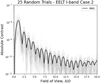 |
Fig. 5 Radial profile of the azimuthally averaged focal plane residuals given the polarization aberrations of spatially-varying coatings on the ELT primary mirror. These data are generated by taking the difference of coronagraphic images with and without segment-to-segment coating variations. These data are computed in I-band for a PC of order 2, and plotted on a log scale to show the change in the absolute value of contrast and highlight the distribution’s features. Each individual trial is plotted in gray, and the RMS of these data is plotted in solid black. |
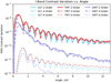 |
Fig. 6 RMS contrast variation as a function of angular separation for Case 2 in I-band. The lines represent the azimuthal average of the standard deviation of the simulated coronagraphic residuals. One can interpret these data as the anticipated contrast degradation due to coating variations. We observe that order 2–4 coronagraphs do not have substantially different performance, with an RMS contrast variation near the inner working angle of ≈10–8 for the TMT and ELT, and ≈5 × 10⁻⁹ for the GMT. Order 6 coronagraphs have a much tighter standard deviation, which is below 10−10 contrast. These data suggest that segment-to-segment errors will not be a dominant effect that limits high-contrast imaging. For the curves that represent Case 1 and 3, please refer to the appendices. |
5 Effect on polarimetry
While the segment-to-segment variations will not be the limiting factor in high-contrast imaging for the GSMTs, another area critical to study is how polarization aberrations from coating variations impact polarimetric observations.
To understand the response of a telescope’s point-spread function to polarization aberrations, we construct the Mueller Point-Response Matrix (MPRM). Using PRT we compute the Jones Pupil J(x, y; θ) in the local coordinate system of the coronagraph, which is computed for some field angle θ. We then propagate J(x, y; θ) through the coronagraph (C) to arrive at the amplitude response matrix Acoro(x′, y′; θ), as shown in Equation (2),
![Mathematical equation: ${{\bf{A}}_{coro}}\left( {x',y';\theta } \right) = {\bf{C}}\left[ {{\bf{J}}(x,y;\theta ){e^{ - i{{{\phi _{xx}} + {\phi _{yy}}} \over 2}}}} \right].$](/articles/aa/full_html/2025/03/aa52671-24/aa52671-24-eq2.png) (2)
(2)
Here (x′, y′) represents the coordinate system of the focal plane, and the exponential term is the phase correction applied by the ideal AO system. The Acoro(x′, y′;θ) is the response of the coronagraphic field, but to understand its influence on the detected intensity, we must transform it to a Mueller matrix. This operation is shown in Equation (3),
 (3)
(3)
Where ⊗ denotes the Kronecker product and U is given by Equation (4),
 (4)
(4)
The Mueller matrix Mcoro describes the response of the focal plane intensity to some incoming Stokes vector S = [I, Q, U, V] T subject to the polarization aberrations present in our instrument. An example of Mcoro is shown in Figure 8, where we show the MPRM for the TMT in I-band. In response to an unpolarized star, i.e. S = [1, 0, 0, 0]T, a detector would measure the top left element of this matrix (I → I). However, in the presence of polarization aberrations some of the unpolarized power I becomes linearly (Q, U) and circularly (V) polarized, which can be detected by polarimeters. This is described by the polar- izance vector of Mcoro, which is the leftmost column of the matrix. Shown in Figure 9 is what a theoretical, uncalibrated, full-Stokes polarimeter would measure from each of the GSMTs in response to an unpolarized star. The polarization aberrations manifest as structure near the inner working angle whose shape and orientation is a function of the incident polarization state. When observing targets at small angular separations to a host star using polarimetric differential imaging, this could be a limiting factor in the best achievable polarimetric contrast.
To best understand the influence of polarization aberrations on the ability to perform high-contrast polarimetry, we consider other extended sources that can be detected in polarized light using polarization differential imaging (PDI). This includes circumstellar disks and reflected light from exoplanets, which may be limited by the structure imparted by the MPRM. In contemporary systems, the influence of first-order polarization aberrations (instrumental polarization, cross-talk) on polarimetry can in part be accounted for using calibration routines.
Calibration routines for current high-contrast polarimeters involve a combination of laboratory characterization, internal source calibration, and on-sky standard observations. Observations of unpolarized and polarized standards can retrieve the retardance and diattenuation of telescope mirrors, while internal calibration sources can determine the polarimetric properties of components downstream of the telescope. All polarizing components are represented as 4 × 4 Mueller matrices, and the overall instrument is represented as the product of such components. To characterize instrumental polarization from the telescope, observations of standard stars at several altitudes on the same night as science observations is a robust method of estimating the mirrors’ physical properties. As is the case with SPHERE-ZIMPOL (Schmid et al. 2018), SPHERE-IRDIS (van Holstein et al. 2020; de Boer et al. 2020), and SCExAO-VAMPIRES (Zhang et al. 2023), internal calibrations are preferably also performed at a regular cadence (e.g. weekly, monthly) to track any changes in polarimetric properties. Using internal-source and on-sky calibration datasets, polarimeters such as SPHERE-IRDIS have achieved absolute polarimetric error on the order of 0.1% (van Holstein et al. 2020) and a polarized contrast of 10–5 – 10–6 (van Holstein et al. 2017). In van Holstein et al. (2021), SPHERE- IRIDIS achieved a 1 – σ polarized contrast of 10–8 at 1.5 arcsec. In this section we construct a model of a debris disk and subject it to the polarization aberrations that arise in segments with coating variations to assess the degree of polarimetric accuracy that needs to be calibrated, and assess the presence of any spatially-varying structure that might arise.
A debris disk model was constructed using the radiative transfer routine MCFOST (Pinte et al. 2006). The model is intended to be an analogue of the HR 4796A debris disk system (e.g., Schneider et al. 1999; Perrin et al. 2015), with a host star (Teff ~ 9250 K) 73 pc away. The model was constructed to have a position angle of 28°, a vertical aspect ratio of 0.01, and a radius of peak dust density of 73.7 au. The radial density profile follows a two power-law structure, simulating a “sharp” inner profile (αin = 9.25) cut-off to 0 at 60 au and a sharp outer profile (αout = –12.25) cut-off at 20 au. We assume compact, spherical Mie-scattering grains (Mie 1908) with 100% astrosilicate composition, a minimum grain size of 1.8 µm, and a distribution of grain sizes following a single power-law function per Dohnanyi (1969). We assume that these dust grains don’t generate circular polarization from physical processes like multiple scattering. We assume an observing wavelength of 860 nm (I-band). MCFOST generates I, Q, and U images of a disk model. To assess the effects of polarization aberrations on our final polarized intensity disk images, we simulate the model with the previously mentioned properties at an inclination of i = 75°. Relative to the size of our detector, we generated smaller disk models to observe any significant effects from closer to the IWA of the coronagraph. In the highly-inclined disk case, the front-side of the disk (side closest to the observer) lies very near the IWA. The injected Stokes image of the disk is shown in Figure 10.
We construct the image of the disk subject to the GSMT polarization aberrations by transforming it via Mcoro produced by the coronagraphic model used in Section 4. However, to account for the shift- variant behavior near the inner working angle of the coronagraph we must simulate a Mcoro for each point in the field of view that we are concerned with modeling and perform an integral transform on the injected Stokes image (Smodel) with Mcoro. We generate a library of Mcoro evaluated at a number of points such that the injected Stokes image of the disk is Nyquist-sampled. The resulting field-dependent integral transform can be represented as sum of matrix-vector multiplications as shown in Equation (5),
 (5)
(5)
where Sconv is the simulated Stokes image with polarization aberration, j, k are the indices of the grid of field points simulated along the x, y axes, and Mcoro, j,k is the MPRM evaluated at the j – th and k – th field point. We simulate the Sconv for each of the GSMTs using this disk model, and construct the normalized Stokes vector sconv for each of them by dividing by the I parameter as shown in Equation (6),
![Mathematical equation: ${{\bf{s}}_{con\v }} = {1 \over {{I_{con\v }}(x,y)}}{{\bf{S}}_{con\v }} = \left[ {1,{q_{con\v }}(x,y),{u_{con\v }}(x,y),{v_{con\v }}(x,y)} \right].$](/articles/aa/full_html/2025/03/aa52671-24/aa52671-24-eq6.png) (6)
(6)
This normalizes the Stokes images to be expressed in terms of the degree of polarization for easy comparison that isn’t a function of the intensity on a particular position on the disk. We then compute the difference of sconv for each of the GSMTs with the normalized input Stokes image smodel to arrive at the difference in the Stokes parameters due to the polarization aberration model subject to segment-to-segment variations. These data are shown in Figure 11.
The lack of higher-order structure in these results shows that polarimetry is clearly dominated by the instrumental polarization and crosstalk of the GSMTs, rather than the segment-to-segment variation. The instrumental polarization of the GMT is highest, showing a strong + Q polarization of the detected disk. This is consistent with the result in Anche et al. (2023) that the GMT is the greatest diattenuator. The linear-to-circular crosstalk is also strongest in the TMT, which we observed in Anche et al. (2023) to be the greatest retarder. The ELT experiences the least amount of both instrumental polarization and crosstalk, but has a similar overall structure to the TMT. The maximum crosstalk experienced by the TMT is at roughly 30% of the degree of polarization, which can substantially limit the sensitivity and accuracy of astronomical polarimeters by rotating the true polarization into the null space of the polarimeter, which typically senses linear light. The increased degree of Q polarization is approximately constant for the GMT, and could in principle be calibrated out. The remaining symmetric errors that are prominent in the ∆U column are on the order of ±4%, and may be indicative of retardance in the instrument that could also be calibrated out. Methods for doing so are covered exhaustively in the literature, which we report earlier in this section. However, the critical takeaway from this analysis is that the polarization aberrations from segment-to-segment variations are not a substantive limiter to polarimetry.
Note that the analysis conducted in this section does not consider the limitations that may be imposed by a bright host star. For example, faint disks will suffer from the residuals in polarized contrast introduced by the spatially-varying polarization near the inner working angle, like that shown in Figure 9. Another interesting phenomenon to explore is how the polarized structure of the MPRM couples into scalar wavefront error, which has been observed on GPI in Millar-Blanchaer et al. (2022a), and theoretically explored for the GSMTs in Ashcraft et al. (2024). An accurate study of these effects is dependent on both the high-contrast imaging system, and target being observed, and will consequently be explored in future work.
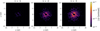 |
Fig. 7 Influence of the Al2O3 layer on coronagraphic performance of the GMT for a 6th-order PC in I-band. These data show the difference between the case with and without segment variations. Here n is the exponent of the PSD used to generate the distribution of Al2O3 on the primary mirror. We observe that the coronagraphic residuals generally increase with decreasing n, but do not exceed 10–9 contrast. |
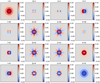 |
Fig. 8 Figure showing the Mueller PRM Mcoro for the TMT in I-band to show how polarization shapes the PSF. A simple imager would observe the I → I component of Mcoro. The data shown here are normalized to the peak of this component. In response to unpolarized light, the observed image of a point-source is simply the sum of the top row times the Stokes vector that represents the source. However, for images that we detect in linear polarized light the U → Q and Q → U retardance terms may sculpt the disk image in a way that inhibits precise detection. The data here is plotted with a colorbar such that bright signals are saturated to enhance the structure in the first lobe of the PRM elements. |
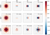 |
Fig. 9 Stokes vectors that would be detected by a perfect high-contrast polarimeter (order = 2 PC) that observed an unpolarized star subject to the polarization aberrations of the GSMTs. These data are normalized to the peak of the I → I component. Each row is a Stokes vector that belongs to one of the GSMTs; (top) TMT, (middle) ELT, (bottom) GMT. These data are plotted on a scale to emphasize the contribution of the polarization aberration to the stellar leakage at the inner working angle. The peak-to-valley (PTV) of the Stokes images is shown on the top-right of each image. Some terms have a PTV larger than 1 because they can take on negative values. |
 |
Fig. 10 Nominal Stokes image of the debris disk model. I is the total intensity, and is plotted on a square root scale to highlight the faint disk features. The linear Stokes parameters Q and U are plotted on a linear scale. The simulated dust grains do not induce circular polarization because we assume that the mechanisms that generate it, like multiple scattering or the presence of magnetic fields, are absent. |
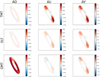 |
Fig. 11 Difference in normalized Stokes parameters with respect to the debris disk model shown in Figure 10. We find that the GMT creates a large difference in the linear Stokes parameter Q, which is consistent with its large diattenuation in I-band that we reported on in Anche et al. (2023). The largest change in the U and V Stokes parameters is from the TMT, which we know exhibits the greatest retardance in I-band. The U difference images are symmetric, indicating a rotation of the detected polarization states observed from the disk. All three GSMTs suffer from a considerable degree of crosstalk, which is shown by the V parameter which has zero input signal. This is readily apparent from the large I → V element of the Mueller PRM shown in Figure 8. |
6 Summary and conclusion
A precise understanding of how polarization aberrations impact the GSMTs is critical for ground-based astronomy at shorter wavelengths. In this study, we present the next step required to bring models of polarization aberrations to higher fidelity.
Below, we summarize the most critical findings from this study into polarization aberrations:
We have added another level of realism to our previously published polarization aberration models of the GSMTs that includes segment-to-segment variations;.
By assuming different spatial distributions of segment-to- segment coating variations on the primary mirror, we are able to statistically sample and parameterize the influence of nonuniform coatings on coronagraphic performance. For the middling case, we determined that the RMS contrast variation does not exceed 2 × 10⁻⁸ contrast for the most sensitive coronagraph (order 2) and worst polarization aberrations (TMT) in I-band. This is orders of magnitude below the AO-limited residuals anticipated for the GSMTs, and will not be a substantive error term;
Our analysis of the coronagraphic residuals is dependent on the assumptions made about the structure of the segment-to- segment variations. Little is known about the actual spatial structure of the coatings deposited on large segments, and their refractive indices and film thicknesses should be measured for a more accurate analysis. However, given the substantial variation in film thickness studied in this work, we do not expect segment-to-segment coating variations to be a limiter in high-contrast imaging for the GSMTs;
We assess the degree to which polarization aberrations from segment-to-segment variations will impact polarimetry of stars and debris disks. Ultimately we find that the coronagraphic Mueller point-response matrix exhibits polarized structure near the inner working angle of the coronagraphs. This means that observations of both unpolarized and polarized stars will have spatially-varying polarized structure near the inner working angle of a coronagraph. This effect does not appear to substantially alter the morphology of polarized off-axis structures like debris disks, whose detection errors are dominated by instrumental polarization and crosstalk;
Our analysis of the influence on polarimetry could be expanded by incorporating these polarization aberration models into end-to-end models of coronagraphs, which will result in a polarized background that could limit polarimetric detection (using PDI) of faint objects like exoplanets;
As part of this paper, we have built a GSMT polarization aberration forward modeling pipeline that is built using Poke’s polarization ray tracing module and the HCIPy physical optics propagation package (Ashcraft 2024);
While the goal of direct exoplanet detection and spectroscopy for the GSMTs may be constrained by the nominal polarization aberrations in the GSMTs, the influence of segment-to-segment coating thickness variations does not contribute a substantive error term to high contrast detection or polarimetry.
We plan to fully integrate our simulations described here into an end-to-end model of a high-contrast imaging instrument planned for the GSMTs. For example, the GMagAO-X instrument (Males et al. 2022) is an extreme-AO system in development that aims to achieve visible to near infrared high-contrast imaging on the GMT to search for planets in reflected light orbiting nearby stars. Similarly, the Planetary Camera and Spectrograph (PCS) is planned for the ELT, and the Planetary Systems Imager is planned for the TMT, both of which will cover similar wavelengths (Kasper et al. 2021; Fitzgerald et al. 2022).
Merging a realistic coronagraph model with our polarization aberration model, and integrating it with an end-to-end Fresnel analysis is the next step toward understanding the precise influence of polarization aberrations from the GSMTs. The intermediate optics and atmospheric residuals will create a speckle field at the focal plane that, due to polarization aberrations, has some degree of polarization (Millar-Blanchaer et al. 2022a; Ashcraft et al. 2024). Studying how this effect can limit wavefront control algorithms is critical to optimizing the science yield of next-generation high-contrast imaging instruments.
Acknowledgements
This work was supported by a NASA Space Technology Graduate Research Opportunity. The authors thank Saeko Hayashi, Ben Gallagher, and Warren Skidmore for helpful discussions about the planned TMT primary mirror segment coatings. S.Y.H acknowledges funding from the Heising Simons Foundations. J.N.A was supported by NASA through the NASA Hubble Fellowship grant #HST-HF2-51547.001-A awarded by the Space Telescope Science Institute, which is operated by the Association of Universities for Research in Astronomy. This research made use of several open-source Python packages, including HCIPy (Por et al. 2018), prysm (Dube et al. 2022), numpy (Harris et al. 2020), matplotlib (Hunter 2007), ipython (Pérez & Granger 2007), and astropy (Astropy Collaboration 2013, 2018, 2022).
Appendix A RMS contrast variations
The RMS contrast variations for Case 1 (Figure A.1) and Case 3 (Figure A.2). As anticipated, Case 1 outperforms Case 2 (Figure 6), and Case 3 underperforms Case 2. Even for the worstcase contrast variation, the RMS Contrast does not exceed 10–7 contrast.
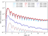 |
Fig. A.1 RMS contrast variation as a function of angle for Case 1 in I-band. The lines represent the azimuthal average of the standard deviation of the simulated coronagraphic residuals. These trends tend to mimic the behavior in Figure 6, but be a factor of 2-5 lower in RMS contrast. |
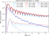 |
Fig. A.2 RMS contrast variation as a function of angle for Case 3 in I-band. The lines represent the azimuthal average of the standard deviation of the simulated coronagraphic residuals. These trends tend to mimic the behavior in Figure 6, but be a factor of 2-5 lower in RMS contrast. |
Appendix B Mueller point-response matrices for the GMT and ELT
Figures illustrating the Mueller point-response matrices for the ELT (Figure B.1) and the GMT (Figure B.2) to illustrate the polarized structure that can arise near the inner working angle of the perfect coronagraph models in the presence of polarization aberration.
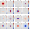 |
Fig. B.1 Figure showing the Mueller PRM Mcoro for the ELT in I-band to show how polarization shapes the PSF. These data are normalized to the peak of the I → I component. The data here is plotted with a colorbar such that bright signals are saturated to enhance the structure in the first lobe of the PRM elements. |
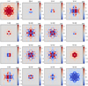 |
Fig. B.2 Figure showing the Mueller PRM Mcoro for the GMT in I-band to show how polarization shapes the PSF. These data are normalized to the peak of the I → I component. The data here is plotted with a colorbar such that bright signals are saturated to enhance the structure in the first lobe of the PRM elements. |
References
- Anche, R. M., Ashcraft, J. N., Haffert, S. Y., et al. 2023, A&A, 672, A121 [NASA ADS] [CrossRef] [EDP Sciences] [Google Scholar]
- Anche, R. M., Douglas, E., Milani, K., et al. 2023a, PASP, 135, 125001 [NASA ADS] [CrossRef] [Google Scholar]
- Anche, R. M., Haffert, S. Y., Ashcraft, J. N., et al. 2023b, in Techniques and Instrumentation for Detection of Exoplanets XI, 12680, SPIE, 248 [Google Scholar]
- Ashcraft, J. 2024, polarization-gsmts-II, https://doi.org/10.5281/zenodo.10800962 [Google Scholar]
- Ashcraft, J. N., Douglas, E. S., Kim, D., et al. 2023, in Optical Modeling and Performance Predictions XIII, 12664, ed. M. A. Kahan, International Society for Optics and Photonics (SPIE), 1266404 [NASA ADS] [Google Scholar]
- Ashcraft, J. N., Millar-Blanchaer, M. A., Douglas, E. S., Anche, R. M., & Hom, J. 2024, in Modeling, Systems Engineering, and Project Management for Astronomy XI, 13099, eds. S. E. Egner, & S. Roberts, International Society for Optics and Photonics (SPIE), 130992F [Google Scholar]
- Astropy Collaboration (Robitaille, T. P., et al.) 2013, A&A, 558, A33 [NASA ADS] [CrossRef] [EDP Sciences] [Google Scholar]
- Astropy Collaboration (Price-Whelan, A. M., et al.) 2018, AJ, 156, 123 [Google Scholar]
- Astropy Collaboration (Price-Whelan, A. M., et al.) 2022, ApJ, 935, 167 [NASA ADS] [CrossRef] [Google Scholar]
- Balasubramanian, K., Hoppe, D. J., Mouroulis, P. Z., Marchen, L. F., & Shaklan, S. B. 2005, in Techniques and Instrumentation for Detection of Exoplanets II, 5905, SPIE, 137 [NASA ADS] [Google Scholar]
- Bishop, N., Walker, J., DeRoo, C. T., et al. 2019, J. Astron. Telesc. Instrum. Syst., 5, 021005 [CrossRef] [Google Scholar]
- Breckinridge, J. B., Lam, W. S. T., & Chipman, R. A. 2015, PASP, 127, 445 [CrossRef] [Google Scholar]
- Breckinridge, J., Kupinski, M., Davis, J., Daugherty, B., & Chipman, R. 2018, in Space Telescopes and Instrumentation 2018: Optical, Infrared, and Millimeter Wave, 10698, SPIE, 429 [Google Scholar]
- Cavarroc, C., Boccaletti, A., Baudoz, P., Fusco, T., & Rouan, D. 2006, A&A, 447, 397 [NASA ADS] [CrossRef] [EDP Sciences] [Google Scholar]
- Chipman, R. A., Lam, W.-S. T., & Young, G. 2018, Polarized Light and Optical Systems (CRC Press) [CrossRef] [Google Scholar]
- de Boer, J., Langlois, M., van Holstein, R. G., et al. 2020, A&A, 633, A63 [NASA ADS] [CrossRef] [EDP Sciences] [Google Scholar]
- Doelman, D. S., Belaouchi, H., Riggs, A., et al. 2023, in Techniques and Instrumentation for Detection of Exoplanets XI, 12680, SPIE, 294 [Google Scholar]
- Dohnanyi, J. 1969, J. Geophys. Res., 74, 2531 [NASA ADS] [CrossRef] [Google Scholar]
- Dube, B. D., Riggs, A. J., Kern, B. D., et al. 2022, J. Opt. Soc. Am. A, 39, C133 [Google Scholar]
- Fitzgerald, M. P., Sallum, S., Millar-Blanchaer, M. A., et al. 2022, SPIE Conf. Ser., 12184, 1218426 [NASA ADS] [Google Scholar]
- Gaudi, B. S., Seager, S., Mennesson, B., et al. 2020, arXiv e-prints [arXiv:2001.06683] [Google Scholar]
- Guyon, O., Pluzhnik, E. A., Kuchner, M. J., Collins, B., & Ridgway, S. T. 2006, ApJS, 167, 81 [NASA ADS] [CrossRef] [Google Scholar]
- Harris, C. R., Millman, K. J., van der Walt, S. J., et al. 2020, Nature, 585, 357 [NASA ADS] [CrossRef] [Google Scholar]
- Hart, J. G. J., van Holstein, R. G., Bos, S. P., et al. 2021, in Polarization Science and Remote Sensing X, 11833, eds. M. K. Kupinski, J. A. Shaw, & F. Snik, International Society for Optics and Photonics (SPIE), 118330O [NASA ADS] [Google Scholar]
- Hunter, J. D. 2007, Comput. Sci. Eng., 9, 90 [NASA ADS] [CrossRef] [Google Scholar]
- Kasdin, N. J., Bailey, V. P., Mennesson, B., et al. 2020, in Space Telescopes and Instrumentation 2020: Optical, Infrared, and Millimeter Wave, 11443, SPIE, 300 [Google Scholar]
- Kasper, M., Cerpa Urra, N., Pathak, P., et al. 2021, The Messenger, 182, 38 [Google Scholar]
- Luo, J., He, X., Fan, K., & Zhang, X. 2020, Opt. Express, 28, 37958 [NASA ADS] [CrossRef] [Google Scholar]
- Males, J. R., Close, L. M., Haffert, S. Y., et al. 2022, in Adaptive Optics Systems VIII, 12185, SPIE, 1381 [Google Scholar]
- Mie, G. 1908, Ann. Phys., 330, 377 [Google Scholar]
- Millar-Blanchaer, M. A., Anche, R. M., Nguyen, M. M., & Maire, J. 2022a, in Ground-based and Airborne Instrumentation for Astronomy IX, 12184, SPIE, 1278 [Google Scholar]
- Millar-Blanchaer, M. A., Anche, R. M., Nguyen, M. M., & Maire, J. 2022b, in Ground-based and Airborne Instrumentation for Astronomy IX, 12184, eds. C. J. Evans, J. J. Bryant, & K. Motohara, International Society for Optics and Photonics (SPIE), 121843X [NASA ADS] [Google Scholar]
- Pérez, F., & Granger, B. E. 2007, Comput. Sci. Eng., 9, 21 [Google Scholar]
- Perrin, M. D., Duchene, G., Millar-Blanchaer, M., et al. 2015, ApJ, 799, 182 [Google Scholar]
- Pinte, C., Ménard, F., Duchêne, G., & Bastien, P. 2006, A&A, 459, 797 [NASA ADS] [CrossRef] [EDP Sciences] [Google Scholar]
- Por, E. H., Haffert, S. Y., Radhakrishnan, V. M., et al. 2018, in Proc. SPIE, 10703, Adaptive Optics Systems VI, 1112 [Google Scholar]
- Sanchez Almeida, J., & Martinez Pillet, V. 1992, A&A, 260, 543 [Google Scholar]
- Sankarasubramanian, K., Samson, J., & Venkatakrishnan, P. 1999, in Solar Polarization: Proceedings of an International Workshop held in Bangalore, India, 12–16 October 1998 (Springer), 313 [Google Scholar]
- Schmid, H. M., Bazzon, A., Roelfsema, R., et al. 2018, A&A, 619, A9 [NASA ADS] [CrossRef] [EDP Sciences] [Google Scholar]
- Schneider, G., Smith, B. A., Becklin, E. E., et al. 1999, ApJ, 513, L127 [Google Scholar]
- Schneider, T., Vucina, T., Hee, C. A., Araya, C., & Moreno, C. 2016, in Groundbased and Airborne Telescopes VI, 9906, eds. H. J. Hall, R. Gilmozzi, & H. K. Marshall, International Society for Optics and Photonics (SPIE), 990632 [NASA ADS] [CrossRef] [Google Scholar]
- van Harten, G., Snik, F., & Keller, C. U. 2009, PASP, 121, 377 [CrossRef] [Google Scholar]
- van Holstein, R. G., Snik, F., Girard, J. H., et al. 2017, in Techniques and Instrumentation for Detection of Exoplanets VIII, 10400, ed. S. Shaklan, International Society for Optics and Photonics (SPIE), 1040015 [NASA ADS] [Google Scholar]
- van Holstein, R. G., Girard, J. H., de Boer, J., et al. 2020, A&A, 633, A64 [NASA ADS] [CrossRef] [EDP Sciences] [Google Scholar]
- van Holstein, R., Stolker, T., Jensen-Clem, R., et al. 2021, A&A, 647, A21 [NASA ADS] [CrossRef] [EDP Sciences] [Google Scholar]
- van Holstein, R. G., Keller, C. U., Snik, F., & Bos, S. P. 2023, A&A, 677, A150 [NASA ADS] [CrossRef] [EDP Sciences] [Google Scholar]
- Will, S. D., & Fienup, J. R. 2019, in Techniques and Instrumentation for Detection of Exoplanets IX, 11117, ed. S. B. Shaklan, International Society for Optics and Photonics (SPIE), 1111710 [NASA ADS] [Google Scholar]
- Zhang, M., Millar-Blanchaer, M., Safonov, B., et al. 2023, in Techniques and Instrumentation for Detection of Exoplanets XI, 12680. ed. G. J. Ruane, International Society for Optics and Photonics (SPIE), 126800S [NASA ADS] [Google Scholar]
This is the default PSD for the SurfaceAberration class in HCIPy.
All Tables
All Figures
|
Fig. 1 Optical layout of the telescopes from Zemax® for the three GSMT’s. The TMT and ELT are cassegrain-type telescopes with a fold mirror configuration, whereas the GMT is Gregorian-type telescope with a fold mirror. |
| In the text | |
|
Fig. 2 Steps to simulate polarimetric imaging of a generally off-axis source in the presence of polarization aberrations through the GSMTs is described here. As a first step, we simulate the segment-to-segment coating variation to be a sum of the piston, tilt, and focus terms of the Zernike polynomials. We then perform the PRT using Poke to estimate Jones pupils for all three telescopes. The Jones pupils and the corresponding low- order polarization aberration terms that are fit to these Jones pupils are available in Anche et al. (2023b). The Jones pupils are propagated through the perfect coronagraphs to calculate the residuals and the peak raw contrast. The Jones pupils are further used to estimate the Amplitude Response Matrix and Mueller Point Response Matrix for use in extended scene simulation. |
| In the text | |
|
Fig. 3 Example of low-order coating variation on the TMT primary mirror. We generate a random set of Zernike coefficients from Z1–Z4 and apply it to each segment using the prysm numerical optics package. The error is normalized to have a peak-to-valley of 10% of the nominal thickness and then added to the nominal thickness. Quantifying the impact of these errors on coronagraphy and polarimetry is important to understanding the as-built performance of the GSMTs. |
| In the text | |
|
Fig. 4 Example of the PSD-generated coating variation assigned on the GMT primary mirror. We generate a power law with a given index n and then enforce its peak-to-valley variation to be consistent with the ±0.08 nm from van Harten et al. (2009). Varying the PSD index n allows us to parameterize the influence of the aluminum oxide layer on the GMT. |
| In the text | |
|
Fig. 5 Radial profile of the azimuthally averaged focal plane residuals given the polarization aberrations of spatially-varying coatings on the ELT primary mirror. These data are generated by taking the difference of coronagraphic images with and without segment-to-segment coating variations. These data are computed in I-band for a PC of order 2, and plotted on a log scale to show the change in the absolute value of contrast and highlight the distribution’s features. Each individual trial is plotted in gray, and the RMS of these data is plotted in solid black. |
| In the text | |
|
Fig. 6 RMS contrast variation as a function of angular separation for Case 2 in I-band. The lines represent the azimuthal average of the standard deviation of the simulated coronagraphic residuals. One can interpret these data as the anticipated contrast degradation due to coating variations. We observe that order 2–4 coronagraphs do not have substantially different performance, with an RMS contrast variation near the inner working angle of ≈10–8 for the TMT and ELT, and ≈5 × 10⁻⁹ for the GMT. Order 6 coronagraphs have a much tighter standard deviation, which is below 10−10 contrast. These data suggest that segment-to-segment errors will not be a dominant effect that limits high-contrast imaging. For the curves that represent Case 1 and 3, please refer to the appendices. |
| In the text | |
|
Fig. 7 Influence of the Al2O3 layer on coronagraphic performance of the GMT for a 6th-order PC in I-band. These data show the difference between the case with and without segment variations. Here n is the exponent of the PSD used to generate the distribution of Al2O3 on the primary mirror. We observe that the coronagraphic residuals generally increase with decreasing n, but do not exceed 10–9 contrast. |
| In the text | |
|
Fig. 8 Figure showing the Mueller PRM Mcoro for the TMT in I-band to show how polarization shapes the PSF. A simple imager would observe the I → I component of Mcoro. The data shown here are normalized to the peak of this component. In response to unpolarized light, the observed image of a point-source is simply the sum of the top row times the Stokes vector that represents the source. However, for images that we detect in linear polarized light the U → Q and Q → U retardance terms may sculpt the disk image in a way that inhibits precise detection. The data here is plotted with a colorbar such that bright signals are saturated to enhance the structure in the first lobe of the PRM elements. |
| In the text | |
|
Fig. 9 Stokes vectors that would be detected by a perfect high-contrast polarimeter (order = 2 PC) that observed an unpolarized star subject to the polarization aberrations of the GSMTs. These data are normalized to the peak of the I → I component. Each row is a Stokes vector that belongs to one of the GSMTs; (top) TMT, (middle) ELT, (bottom) GMT. These data are plotted on a scale to emphasize the contribution of the polarization aberration to the stellar leakage at the inner working angle. The peak-to-valley (PTV) of the Stokes images is shown on the top-right of each image. Some terms have a PTV larger than 1 because they can take on negative values. |
| In the text | |
|
Fig. 10 Nominal Stokes image of the debris disk model. I is the total intensity, and is plotted on a square root scale to highlight the faint disk features. The linear Stokes parameters Q and U are plotted on a linear scale. The simulated dust grains do not induce circular polarization because we assume that the mechanisms that generate it, like multiple scattering or the presence of magnetic fields, are absent. |
| In the text | |
|
Fig. 11 Difference in normalized Stokes parameters with respect to the debris disk model shown in Figure 10. We find that the GMT creates a large difference in the linear Stokes parameter Q, which is consistent with its large diattenuation in I-band that we reported on in Anche et al. (2023). The largest change in the U and V Stokes parameters is from the TMT, which we know exhibits the greatest retardance in I-band. The U difference images are symmetric, indicating a rotation of the detected polarization states observed from the disk. All three GSMTs suffer from a considerable degree of crosstalk, which is shown by the V parameter which has zero input signal. This is readily apparent from the large I → V element of the Mueller PRM shown in Figure 8. |
| In the text | |
|
Fig. A.1 RMS contrast variation as a function of angle for Case 1 in I-band. The lines represent the azimuthal average of the standard deviation of the simulated coronagraphic residuals. These trends tend to mimic the behavior in Figure 6, but be a factor of 2-5 lower in RMS contrast. |
| In the text | |
|
Fig. A.2 RMS contrast variation as a function of angle for Case 3 in I-band. The lines represent the azimuthal average of the standard deviation of the simulated coronagraphic residuals. These trends tend to mimic the behavior in Figure 6, but be a factor of 2-5 lower in RMS contrast. |
| In the text | |
|
Fig. B.1 Figure showing the Mueller PRM Mcoro for the ELT in I-band to show how polarization shapes the PSF. These data are normalized to the peak of the I → I component. The data here is plotted with a colorbar such that bright signals are saturated to enhance the structure in the first lobe of the PRM elements. |
| In the text | |
|
Fig. B.2 Figure showing the Mueller PRM Mcoro for the GMT in I-band to show how polarization shapes the PSF. These data are normalized to the peak of the I → I component. The data here is plotted with a colorbar such that bright signals are saturated to enhance the structure in the first lobe of the PRM elements. |
| In the text | |
Current usage metrics show cumulative count of Article Views (full-text article views including HTML views, PDF and ePub downloads, according to the available data) and Abstracts Views on Vision4Press platform.
Data correspond to usage on the plateform after 2015. The current usage metrics is available 48-96 hours after online publication and is updated daily on week days.
Initial download of the metrics may take a while.