| Issue |
A&A
Volume 666, October 2022
|
|
|---|---|---|
| Article Number | A91 | |
| Number of page(s) | 10 | |
| Section | Astronomical instrumentation | |
| DOI | https://doi.org/10.1051/0004-6361/202243413 | |
| Published online | 13 October 2022 | |
Redundant apodization for direct imaging of exoplanets
II. Application to island effects
1
Univ. Grenoble Alpes, CNRS, IPAG,
38000
Grenoble, France
e-mail: lucie.leboulleux@univ-grenoble-alpes.fr
2
Université Côte d’Azur, Observatoire de la Côte d’Azur, CNRS, Laboratoire Lagrange,
06108
Nice, France
3
LESIA, Observatoire de Paris, Université PSL, CNRS, Sorbonne Université, Université de Paris,
5 place Jules Janssen,
92195
Meudon, France
4
Department of Astronomy, California Institute of Technology,
Pasadena, CA
91125, USA
5
Aix Marseille Université, CNRS, LAM (Laboratoire d’Astrophysique de Marseille) UMR 7326,
13388
Marseille, France
6
European Southern Observatory (ESO),
Karl-Schwarzschild-Str. 2,
85748
Garching bei Muenchen, Germany
Received:
24
February
2022
Accepted:
21
May
2022
Context. Telescope pupil fragmentation from spiders generates specific aberrations that have been observed at various telescopes and are expected on the 30-meter class telescopes under construction. This is known as the island effect, and it induces differential pistons, tips, and tilts on the pupil petals, deforming the instrumental point spread function (PSF); it is one of the main limitations to the direct detection of exoplanets with high-contrast imaging. These petal-level aberrations can have different origins such as the low-wind effect or petaling errors in the adaptive optics reconstruction.
Aims. In this paper, we propose a method for alleviating the impact of the aberrations induced by island effects on high-contrast imaging by adapting the coronagraph design in order to increase its robustness to petal-level aberrations.
Methods. Following a method first developed and applied on robustness to errors due to primary mirror segmentation (e.g., segment phasing errors, missing segments), we developed and tested redundant apodized pupils (RAP): apodizers designed at the petal-scale, then duplicated and rotated to mimic the pupil petal geometry.
Results. We applied this concept to the ELT architecture, made of six identical petals, to yield a 10−6 contrast in a dark region from 8 to 40λ/D. Both amplitude and phase apodizers proposed in this paper are robust to differential pistons between petals, with minimal degradation to their coronagraphic PSFs and contrast levels. In addition, they are also more robust to petal-level tip-tilt errors than classical apodizers designed for the whole pupil, with which the limit of contrast of 10−6 in the coronagraph dark zone is achieved for constraints up to 2 rad RMS of these petal-level modes.
Conclusions. In this paper the RAP concept proves its robustness to island effects (low-wind effect and post-adaptive optics petaling), with an application to the ELT architecture. It can also be considered for other 8- to 30-m class ground-based units such as VLT/SPHERE, Subaru/SCExAO, GMT/GMagAO-X, and TMT/PSI.
Key words: atmospheric effects / turbulence / instrumentation: high angular resolution / techniques: high angular resolution / telescopes / planets and satellites: detection
© L. Leboulleux et al. 2022
 Open Access article, published by EDP Sciences, under the terms of the Creative Commons Attribution License (https://creativecommons.org/licenses/by/4.0), which permits unrestricted use, distribution, and reproduction in any medium, provided the original work is properly cited.
This article is published in open access under the Subscribe-to-Open model. Subscribe to A&A to support open access publication.
1 Introduction
The direct imaging and spectroscopy of exoplanets has pushed forward the development of high-contrast imagers set up on large telescopes: the Spectro-Polarimetric High-contrast Exoplanet REsearch instrument (SPHERE) at the Very Large Telescope (VLT), the Gemini Planet Imager (GPI) at the Gemini South Observatory, and the Subaru Coronagraphic Extreme Adaptive Optics (SCExAO) at the Subaru Telescope (Beuzit et al. 2019; Macintosh et al. 2015; Jovanovic et al. 2015). The coming years will witness the development of, among others, the Mid-infrared ELT Imager and Spectrograph (METIS; Kenworthy et al. 2016; Brandl et al. 2018), the High Angular Resolution Monolithic Optical and Near-infrared Integral field spectrograph (HAR-MONI; Carlotti et al. 2019; Thatte et al. 2021; Houllé et al. 2021), and the Multi-AO Imaging Camera for Deep Observations (MICADO; Clénet et al. 2019; Davies et al. 2021) at the Extremely Large Telescope (ELT) and the upgrades of existing instruments like SPHERE+ (VLT, 2025; Boccaletti et al. 2020) and GPI2.0 (Chilcote et al. 2020).
However, instruments already in operation, such as VLT/SPHERE or Subaru telescope/SCExAO have been proved sensitive to a specific aberration called the low-wind effect (LWE), a phenomenon that happens for high-emissivity spider telescopes when the wind speed at the level of the telescope aperture is lower than a few m/s (Sauvage et al. 2015; Milli et al. 2018; Vievard et al. 2019; Holzlöhner et al. 2021), which becomes dominant under good observing conditions (low seeing). With LWE the phase is fragmented into differential piston, tip, and tilt on the pupil petals delimited by the spiders that cannot be corrected by traditional adaptive optics (AO) systems (N’Diaye et al. 2018). It therefore strongly degrades AO-corrected images and impacts coronagraph performance. On noncoronagraphic images, secondary lobes (from one to the number of pupil petals) appear around the location of the first Airy ring, forming what is known as the Mickey Mouse effect illustrated in Fig. 1 (Sauvage et al. 2015; Lamb et al. 2017; Milli et al. 2017). These secondary lobes act like off-axis sources on coronagraphic systems, and can create a severe starlight leakage through the focal-plane mask. The contrast is then degraded at short separations. On SPHERE, where the LWE is one of the main limitations with a phase error of about 200nm RMS (Sauvage et al. 2015, 2016; Cantalloube et al. 2019), the contrast is degraded by a factor of about 50 at 0.1″, and the spider diffraction patterns usually masked by the Lyot stop remain visible up to several arcseconds. In addition, spider diffraction spikes are also visible out of the AO correction area. In 2017, a specific coating with a low thermal emissivity in the mid-infrared was applied on the spiders of the Unit Telescope (UT) 3 of the VLT, but despite a drastic decrease in the aberration amplitude, the LWE still impacts the coronagraphic performance, necessitating the implementation of additional mitigation strategies (Wilby et al. 2018; Vievard et al. 2019; Bos et al. 2020; Pourré et al., in prep.).
The LWE is also expected on upcoming giant telescopes like the ELT (51 cm spider) and the Thirty Meter Telescope (TMT, 225 mm spider; Holzlöhner et al. 2021). In addition, other island phenomena are expected, in particular the petaling effect. This happens when the width of the spiders is greater than the Fried parameter r0 of the atmospheric turbulence at the sensing wavelength. The AO wavefront sensor mistakenly reconstructs discontinuities along the spiders and in particular petal-level pistons (Schwartz et al. 2018; Bertrou-Cantou et al. 2022). These two aberrations, low-wind effect and petaling, will be the focus of this paper.
In this paper, we propose a method to adapt the pupil apodization according to its segmentation by the spiders to make it robust to differential piston, tip, and tilt errors between the pupil petals. This concept derives from the redundant apodized pupil (RAP) coronagraphs, developed and tested in Leboulleux et al. (2022) for errors due to primary mirror segmentation In Sect. 2, we summarize the island effects expected on the ELT. In Sect. 3, we present a short review of the RAP design methodology and concept and extend and apply it in Sect. 4 to the ELT pupil to propose alternative apodizers robust to LWE and post-AO petaling. Another short application of this concept to the TMT aperture is also proposed in Appendix A.
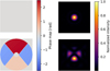 |
Fig. 1 Illustration of the Mickey Mouse effect at a VLT-like configuration (left) Aberration maps applied on the pupil; (right) Associated PSFs in linear scale without aberration (top) and with 415 nm RMS of piston error on the petals (bottom). |
Specifications for four cases: HSP1 and HSP2 (specifically designed by A.
2 Low-wind Effect and Petaling Effect
Island effects can be classified by their sources: (1) the low-wind effect, due to a differential thermal cooling on each side of the spiders and generates petal-level pistons, tips, and tilts, with typical lifetimes of ~2–3 s (Milli et al. 2018), and (2) post-AO petaling, due to the inability of the wavefront sensor to reconstruct wavefront continuities when the spiders are much thicker than the atmosphere spatial coherence length r0, which generates petal-level pistons with a typical lifetime of 1 s (Bertrou-Cantou et al. 2020; see also Sect. 4.2.3 for petaling-induced piston sequences). These lifetimes, if different from the lifetimes of other aberrations (for instance noncommon path aberrations, e.g. Vigan et al. 2022), can increase the complexity of the wavefront reconstruction and correction.
The ELT, with its 51 cm spiders, might be subject to these island effects. While the low-wind effect has mainly been studied on existing telescopes like VLT or Subaru, studies are also ongoing for the ELT (Holzlöhner et al. 2021); in this paper we assume that LWE has the same properties as those observed on SPHERE (i.e., primarily consisting of differential pistons, tips, and tilts). On the other hand, petaling has mainly been studied in simulation and appears as a strong limitation for HARMONI and MICADO, which use visible pyramid wavefront sensors (Schwartz et al. 2018; Bertrou-Cantou et al. 2022).
For both direct and coronagraphic images, these island effects deteriorate the contrast performance. Figure 2 shows the PSFs without and with the low-wind effect, at a level equivalent to that observed on SPHERE before the 2017 spider coating (here ~110 nm RMS of piston and ~ 180 nm RMS of tip and tilt at 1.6 µm; Pourré et al., in prep.), and for three different configurations: without coronagraph, and with the HSP1 and HSP2 shaped pupils (SPs), both designed for the HARMONI high-contrast module (HCM; Carlotti et al. 2018a; Hénault et al. 2018). Both coronagraphs are capable of reaching a contrast limit of 10−6 from 5 to 11λ/D for HSP1 and from 7.5 to 40λ/D for HSP2 (see Table 1). These aberrations create spider diffraction spikes that deteriorate the AO correction area, mainly in the high-contrast dark zone, with an impact on the overall contrast, and particularly on contrast at small angular separations.
For detections limited by speckle noise, for instance when combined with reference star differential imaging (RDI; Lafrenière et al. 2009; Soummer et al. 2012; Gerard & Marois 2016) and angular differential imaging (ADI; Marois et al. 2006), static and quasi-static aberrations must also be strictly controlled with the adaptive optics loop. Due to the difference in evolution lifetimes between dynamic adaptive optics residuals and noncommon path aberrations that require an additional wavefront sensor, island effects can limit the detection unless a specific mitigation tool is provided.
Most mitigation strategies rely on an efficient estimation of the island effect phase errors. To date, different wavefront sensors have been tested: the pyramid wavefront sensor in visible light appears blind to such errors in simulation (Bertrou-Cantou et al. 2022), while the Shack-Hartmann sensor cannot measure petal-level piston errors (Sauvage et al. 2016; Pourré et al., in prep.), even as promising work is ongoing for the estimation of tip-tilt errors in the context of SPHERE and GRAVITY+ (Pourré et al., in prep.). The Zernike sensor for Extremely Low-level Differential Aberrations (ZELDA) has successfully been tested on SPHERE to detect and calibrate the low-wind effect (Sauvage et al. 2015; N’Diaye et al. 2016). Last but not least, several focal-plane wavefront sensors have been tested in simulation, at Subaru, Keck, and the VLT. Phase diversity algorithms, from classical methods (Lamb et al. 2016, 2017) to more complex extensions like the Fast & Furious algorithm (Korkiakoski et al. 2014; Wilby et al. 2016, 2018) have proven to be efficient in estimating low-wind effect phase errors on SPHERE. On SCExAO, the low-wind effect has already been studied with the asymmetric pupil Fourier focal-plane wavefront sensor (Martinache 2013; N’Diaye et al. 2018; Vievard et al. 2019). On SCExAO, the linearized analytic phase diversity technique and again the Fast & Furious algorithm (Vievard et al. 2019) have also been implemented The last mitigation technique does not include any wavefront sensors and consists of the application of a coating with low thermal emissivity in the mid-infrared on the spiders to physically reduce thermal gradients (Milli et al. 2018).
For petaling compensation, except for an infrared pyramid sensor for the METIS AO system (Hippler et al. 2019), Schwartz et al. (2018) proposes an update of the AO correction loop called the edge actuator coupling that consists in considering actuators on each side of the spider as one single actuator to force the system to limit differential pistons between petals. Bertrou-Cantou et al. (2020, 2022) also proposes an update of the reconstruction mode basis to force the phase continuity between petals. Moreover, Hutterer et al. (2018) proposes a split approach with a separated reconstruction of petal-level pistons and of other modes using Bayesian statistics.
This paper investigates a different mitigation strategy, with an adaptation of the RAP design proposed in Leboulleux et al. (2022). All the island effects mentioned earlier are considered as differential pistons between petals, with tips and tilts in the low-wind effect case, and with a quite slow dynamic evolution (one to a few seconds).
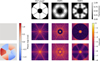 |
Fig. 2 Low-wind effect on the ELT. (top) Three pupil configurations with the full ELT pupil and the shaped pupils HSP1 and HSP2 of HAR-MONI/HCM, and their associated PSFs in logarithmic scale without low-wind effect (center) and with the low-wind effect phase map of the left column (bottom). The phase map is composed of petal-level pistons, tips, and tilts with average values and variances equivalent to those of VLT/SPHERE before the spider coating (here ~110 nm RMS of piston and ~180 nm RMS of tip and tilt at 1.6 µm). |
3 Review of Redundant Apodized Pupils
For segmented telescopes equipped with high-contrast imagers, the Pair-based Analytical model for Segmented Telescopes Imaging from Space (PASTIS, Leboulleux et al. 2018; Laginja & Leboulleux 2019; Laginja et al. 2021) provides an expression for the intensity in the coronagraphic dark hole as a function of the segment-level phase errors. For a symmetric dark zone with amplitude aberrations and phase aberrations after the focal plane mask of the coronagraph neglected, then the intensity in the dark zone I can be expressed as
 (1)
(1)
where nseg is the number of segments in the primary mirror, u is the position vector on the detector,  is the Fourier transform of the Zernike polynomial Z considered as segment-level aberrations,
 ![${({c_k})_{k \in \left[ {1,{n_{{\rm{seg}}}}} \right]}}$](/articles/aa/full_html/2022/10/aa43413-22/aa43413-22-eq3.png) are calibration coefficients including the effect of the coronagraph,
are calibration coefficients including the effect of the coronagraph, ![${\left( {{a_k}} \right)_{k \in \left[ {1,{n_{{\rm{seg}}}}} \right]}}$](/articles/aa/full_html/2022/10/aa43413-22/aa43413-22-eq4.png) are the local Zernike coefficients on the segments, and
are the local Zernike coefficients on the segments, and ![${\left( {{r_k}} \right)_{k \in \left[ {1,{n_{{\rm{seg}}}}} \right]}}$](/articles/aa/full_html/2022/10/aa43413-22/aa43413-22-eq5.png) correspond to the positions vectors from the center of the pupil to the centers of the segments.
correspond to the positions vectors from the center of the pupil to the centers of the segments.
This equation corresponds to a low-order envelope  multiplied by interference fringes between all pairs of segments. For piston-like aberrations, this low-order envelope, also called the halo in Yaitskova & Dohlen (2002); Yaitskova et al. (2003) corresponds to the point spread function (PSF) of the segment. The full pupil PSF can then be seen as the segment PSF modulated by the interference fringes between all pairs of segments. The image intensity at each point is proportional to this segment PSF (or low-order envelope).
The RAP concept of Leboulleux et al. (2022) consists in apodizing each segment to dig a dark hole in the low-order envelope. Since the image corresponding to the full segment pupil is proportional to the segment PSF, it also deepens the contrast in the segmented pupil coronagraphic PSF. It implies that for a given target contrast in the dark zone I, the piston-level error amplitudes ![${\left( {{a_k}} \right)_{k \in \left[ {1,{n_{{\rm{seg}}}}} \right]}}$](/articles/aa/full_html/2022/10/aa43413-22/aa43413-22-eq7.png) can be larger if the low-order envelope
can be larger if the low-order envelope  is reduced (see Eq. (1)), meaning an increased robustness to segment-level aberrations.
In Leboulleux et al. (2022) the RAP concept is applied on errors due to the segmentation of the primary-mirror, on a Giant Magellan telescope-like pupil combined with an apodized pupil Lyot coronagraph (APLC; e.g., Soummer et al. 2009; N’Diaye et al. 2015b; Zimmerman et al. 2016) on the one hand, and with an apodizing phase plate (APP) coronagraph (e.g., Codona 2007; Kenworthy et al. 2010; Carlotti 2013; Por 2017) on the other. RAPs deliver an increased robustness, although at more modest angular separations than targeted by exo-Earth-imagers. Another advantage is that the RAP is a passive component that does not require an additional wavefront sensor or wave-front control tool, such as a deformable mirror, to reduce the constraints on the optical wavefront.
We propose considering the petals delimited by the secondary mirror spiders as pupil segmentation; the low-wind effect as segment-level piston, tip, and tilt errors; and post-AO petaling as segment-level piston errors. With these conditions the RAP concept can be extended and applied to generate coronagraphs robust to island effects, and in the next section we focus on ELT applications. Its six petals are identical, a configuration fitting with the RAP procedure.
When computing a coronagraph apodization it is common to reduce the computational burden of the apodization optimization by apodizing only one-quarter of the pupil when it has a two-axis symmetry (Por et al. 2020; Carlotti et al. 2014). The full pupil PSF can then be numerically computed from one-quarter of the pupil only, and the apodization obtained on one-quarter from this optimization process is then unfolded to obtain the full pupil apodization. The RAP procedure, with an optimization by petal, should not be compared to this numerical trick: it aims at improving the contrast in the low-order envelope instead of the full pupil PSF, and the full pupil PSF is never computed in the apodization optimization process.
4 Application to the Island Effect Mitigation on the ELT
4.1 Apodizer Design
4.1.1 Requirements and Methodology
The objective is to design both amplitude, using SP (Vanderbei et al. 2003; Kasdin et al. 2003; Carlotti et al. 2011), and phase, using APP (Codona 2007; Kenworthy et al. 2010; Carlotti 2013; Por 2017), at the scale of one petal and to reproduce them to cover the entire ELT pupil.
The apodization problem consists of minimizing the intensity in the defined dark region by exploring the parameter space of the petal apodization while maximizing the throughput of the final apodizer. As in Leboulleux et al. (2022), it is formulated in A Mathematical Programming Language (AMPL; Fourer et al. 2002), and the procedure then calls for the Gurobi solver to find the optimal solution (Gurobi Optimization, LLC 2021).
On the HCM of HARMONI, two designs were selected, HSP1 and HSP2 (see Fig. 2), whose specifications (inner working angle, IWA; outer working angle, OWA; and contrast) are given in Table 1 (Carlotti et al. 2018a). The requirements for the RAP designs are equivalent to those of HSP2: set to the deepest contrast of 10−6 from 8 to 40λ/D, where λ is the wavelength (later on set to 1.6 µm) and D the pupil diameter (39m; see also Table 1).
Because there are approximately 2.4 petals along the ELT pupil diameter, these requirements correspond to a dark zone between 3.5 and 16.3λ/d for the petal low-order envelope, where d is the size of the petal. As in Leboulleux et al. (2022), accessing smaller IWAs imposes a drastic decrease in planet throughput and pupil transmission; an IWA of 3.5λ/d was the best compromise found for this application.
Throughputs and transmissions of the three apodizers.
4.1.2 Amplitude Apodizer (SP)
The petal amplitude apodization issued from the AMPL procedure is visible in Fig. 3 (left), as is its PSF, which is also the low-order envelope of the full RAP. This latter is obtained by rotating the petal apodizer around the pupil center by angular steps of 60°. The output design and its PSF are also shown in Fig. 3 (right). We observe that the petal apodizer PSF does not require the contrast constraint to be set at 10−6, 10−5.25 in the petal PSF dark zone being sufficient to obtain a 10−6 contrast on the final RAP PSF dark zone. The intensity profile of the designed apodizer is also shown in Fig. 4 (red).
Table 2 also presents the throughputs T (with respect to the definition of Ruane et al. 2018) and transmissions t of the final designs, which are lower than the corresponding values for HSP2 and defined as
 (2)
(2)
with RAP the RAP function (full apodizer with 0 if no transmission, 1 if transmission), P the entrance pupil function, A a 0.7λ/D radius circular area centered on the star image, Ic the coronagraphic image, and Inc the noncoronagraphic image.
4.1.3 Phase Apodizer (APP)
Figure 5 shows the petal phase apodization computed by the AMPL code, and its associated PSF. Once again, the RAP is designed from six rotations of this petal-level apodizer, also visible in the figure with its PSF. The final design reaches the target contrast of 10−6 between 8 and 40λ/D; the throughput and transmission values are given in Table 2. The 100% transmission in this case does not reflect the loss of planetary photons despite the lack of amplitude apodization, and the transmission value should be ignored. The throughput brings more accurate information about the ratio of planetary photon loss. Patterns close to the IWA are visible on the RAP PSF, with a local contrast slightly above 10−6; similar effects have been obtained for other designs with different specifications. The intensity profile of the output is also shown in Fig. 4 (green); the slight deterioration of contrast is due to the patterns close to the IWA visible around 8–11λ/D. These residuals are probably due to the diffraction by the edge of the petal and are already present in the single petal image. They are also visible in all alternative designs conducted for this study with petal-level APP.
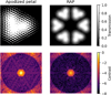 |
Fig. 3 Amplitude apodizations for a single petal (left) and for the full RAP (right). Top: with pupil transmissions from 0 (no transmission) to 1 (full transmission), aiming for a contrast of 10−6 between 8 and 40λ/D. Bottom: associated PSFs in logarithmic scale. |
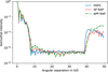 |
Fig. 4 Coronagraphic intensity profiles, normalized to the intensity peak, of one of the two shaped pupils designed for the HARMONI configuration (HSP2 in blue), and the two RAPs presented in this paper: the amplitude RAP (red) and the phase RAP (green). The three designs aim for 10−6 contrasts in their dark zones (see Table 1). |
4.2 Robustness to Island Effects
Since the RAPs are optimized to be robust to piston-like errors between petals, we separately examine their robustness to piston and tip-tilt errors.
4.2.1 Petal-level Piston Errors
Figure 6 (top two lines) shows the PSFs without and with pistons between the pupil petals for the three different apodizers considered here. The amplitudes of the pistons have been chosen with the same statistics (average and variance) as was observed on the SPHERE instrument before the 2017 spider coating. The PSFs from the two RAPs do not appear to be impacted, while strong leakage appears on the PSF behind HSP2.
More generally, it is possible to compute the average contrast in the dark zone as a function of the amplitude of the aberrations for a wide range of aberrations. In Fig. 7, amplitudes of aberrations between 1 mrad and 10 rad are considered, and for each amplitude 100 random phase maps are simulated and propagated through the coronagraph. For each error amplitude, the average of the 100 mean contrasts is computed and appears on this curve. All apodizers have been designed to access a maximum contrast in their dark zone of 10−6, while these curves indicate the average contrast in the dark zone, which accounts for the values of the plots below 10−6 for small wavefront error amplitudes. It is noticeable that the two RAP designs show a quite stable performance that remain below 10−6 despite the increasing aberrations, and they stabilize around 7 × 10⁻⁷ for aberrations up to 1 rad RMS, while the HSP2 performance starts to be impacted around 200 mrad RMS. In particular, the deterioration of contrast at large amplitude aberrations reflects the loss of coherence in the planet image (above 1 rad).
The PSF deterioration by petal-level piston errors is localized along the axes perpendicular to the spider shadows and more impacted at small angular separations than farther from the optical axis. This localized effect is not fully captured by the metric chosen in Fig. 7, which is computed over the entire dark zone.
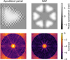 |
Fig. 5 Phase apodizations for a single petal (left) and for the full RAP (right). Top: pupil phases in radians, aiming for a contrast of 10−6 between 8 and 40λ/D. Bottom: associated PSFs in logarithmic scale. |
4.2.2 Petal-level Tip-tilt Errors
In Fig. 6 (third line), PSFs in the presence of only petal-level tip-tilt aberrations are also presented for the three apodizers considered in this study. As in the previous section, the tip-tilt amplitudes were randomly selected with average and variances equivalent to the values recorded on SPHERE before the 2017 spider coating (Pourré et al., in prep.). In the HSP2 case, petal tips and tilt appear to have a similar effect to the petal pistons (i.e., starlight leakage along the spider diffraction spikes). In the RAP cases though these spikes are milder.
To verify this assumption, we compute the evolution of the average contrast in the dark zone for a large range of petal-level tip-tilt amplitudes. As above, amplitudes from 1mrad to 10 rad are considered, and for each amplitude 100 random phase maps are computed and propagated through the coronagraph, the average value of the 100 associated contrasts are plotted in Fig. 8. The average contrasts reach 10−6 at respectively 0.48, 2.3, and 2.4rad RMS for the HSP2, SP RAP, and APP RAP designs. The impact of petal-level errors on the coronagraphic PSF is lower for tip-tilt than for piston for the HSP2 design, with local pistons remaining the strongest limitation to the performance.
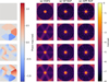 |
Fig. 6 Robustness to low-wind effect errors between petals. Left: phase maps simulated in the pupil plane in radians. Right: associated PSFs in logarithmic scale with the three designs. Four phases are considered (from top to bottom): no error; piston-only errors, at the level observed on SPHERE before coating; tip-tilt-only errors, also at the SPHERE level; combined piston-tip-tilt errors from the above lines. |
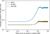 |
Fig. 7 Evolution of the contrast with the piston-like low-wind effect errors between petals with the HSP2 design (blue), the amplitude RAP design (red), and the phase RAP design (green). For each amplitude error considered here, 100 random phase maps are simulated and propagated through the coronagraph, and the average of the 100 contrasts is plotted here. |
4.2.3 Post-OA Petaling
Post-AO system petaling is also expected at the ELT, particularly for the MICADO and HARMONI instruments. We propose studying its effect on the coronagraphic performance for different conditions and correction methods, with the AO specifications described in (Bertrou-Cantou et al. (2022, Table 1): a 500 Hz loop rate with a visible light (700 nm) pyramid wavefront sensor and a 5352 actuator deformable mirror.
The first considered conditions correspond to a Fried parameter r0 = 12.8 cm at 500 nm (Q3 conditions as defined by the European Southern Observatory, ESO). The AO system generates differential pistons between segments, plotted in Fig. 9 (top). The data is issued from the COMputing Platform for Adaptive opticS System (COMPASS) end-to-end simulation software (Ferreira et al. 2018b,a; Conan et al. 2005). Figure 9 (bottom) also presents the average contrasts in their dark zones behind the different coronagraphs considered in this paper.
However, compensation methods are planned to correct for these differential pistons. Figure 10 (top) indicates the differential pistons with the same turbulence sequence as in Fig. 9, but the AO system is coupled with continuity hypotheses between petals (Bertrou-Cantou et al. 2020). Figure 10 (bottom) shows the average dark zone contrasts behind the three apodizers.
The RAPs are also tested in milder conditions with a Fried parameter r0 = 21.5 cm at 500 nm (Q1 conditions as defined by ESO). We consider an AO correction, combined once again with continuity hypotheses between petals. Figure 11 presents the differential pistons issued from COMPASS, in addition to the average contrasts in the coronagraphic dark zones.
The RAP designs show significant robustness with no contrast deterioration to post-AO petaling effects in various atmospheric turbulence conditions. They also have no particular requirement for additional tools such as continuity hypotheses between petals since their average contrast remains below 10−6 both without and with these hypotheses.
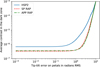 |
Fig. 8 Evolution of the contrast with the tip-tilt-like low-wind effect errors between petals with the HSP2 design (blue), the amplitude RAP design (red), and the phase RAP design (green). For each amplitude error considered here 100 random phase maps are simulated and propagated through the coronagraph, and the average of the 100 contrasts is plotted here. |
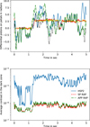 |
Fig. 9 Impact of the petaling on the coronagraphic performance. Top: differential piston sequence in radians over 5 s for five petals, the sixth being the reference, for r0 = 12.8 cm conditions and behind the AO system. Bottom: average contrasts of the three coronagraphs considered in this paper. |
4.3 Robustness to other Low-order Aberrations
In this section, we focus on typical alignment errors, expressed as the first Zernike polynomials, and test the robustness of the three coronagraph designs.
Figure 12 shows the coronagraphic PSFs for the first Zernike polynomials; each one is normalized at 0.25λ RMS on a circular support. These aberrations are low order, and mainly modify the shape of the PSF central core in a similar way for the three designs. Since they have an impact close to the optical axis, they correspond to a loss in performance at small angular separations (i.e., an increase in IWA). Despite little to no impact in the dark zone far from the optical axis, the three designs suffer from a similar contrast loss at small angular separations.
In addition, aberrations that impact the coronagraphic PSF at angular separations smaller than the IWA decrease the Strehl ratio by modifying the PSF central core. This Strehl ratio decrease translates into a uniform contrast loss for the entire dark zone, which also appears in Fig. 12 with an equivalent impact for the three designs.
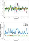 |
Fig. 10 Impact of the petaling on the coronagraphic performance. Top: Differential piston sequence in radians over 5 s for five petals, the sixth being the reference, for r0 = 12.8 cm conditions, behind the AO system and combined with continuity hypotheses between petals. Bottom: average contrasts of the three coronagraphs considered in this paper. |
5 Conclusions
This paper follows up on a first introduction to the RAP component in Leboulleux et al. (2022), which was then developed to design coronagraphs robust to errors due to primary mirror segmentation. In this second paper we propose an extension of this technique to island effects (low-wind effect and post-AO petaling).
Redundant apodized pupils applied to the island effect are designed by generating an apodizer for one petal only and reproducing it over the other petals to mimic the pupil discontinuity. In this paper it is applied to the ELT pupil to design both amplitude and phase apodizers (SP and APP) that create dark zones down to 10−6 between 8 and 40λ/D. The resulting apodizers appear extremely robust to petal-level piston errors over the entire range of considered aberrations (1 mrad RMS to 10 rad RMS) and are also highly robust to petal-level tip-tilt errors, with constraints of around 2rad RMS for average contrasts in the dark zone of 10−6.
Similarly to what has been observed in Leboulleux et al. (2022), RAPs do not allow for IWAs as low as classical apodizers since they are limited by the petal diffraction limit: HSP1 and HSP2 can access angular separations down to 5 and 7.5λ/D, respectively, versus 8λ/D for both RAPs. For instance, a 7λ/D IWA translates into an important loss of throughput compared to a 8λ/D IWA, from 24% to 11% in the SP RAP case. However, two-step strategies (possibly optimized simultaneously) can be implemented.
For a higher contrast limit, the first step is needed to generate a RAP at an intermediate contrast but at a high throughput and/or a small IWA, then the second step updates the apodization on the overall pupil to increase the contrast performance. This would translate into a lower loss in throughput than with the fully redundant apodization and a lower loss in robustness than only with the full aperture (nonredundant) apodization. This aspect is similar to the apodized pupil Lyot coronagraph designs of Leboulleux et al. (2022), which led to a higher contrast than that accessible only with the RAP, but to a loss in robustness.
For access to small angular separations, the first step obtains a RAP at the target contrast but higher IWA than the target’s IWA to limit the throughput loss; the second step updates the apodization to access a smaller IWA. Since this second step apodization is not fully redundant for low-order apodization patterns, it would also translate into a loss in robustness at small angular separations.
In addition, complex RAPs could also be considered to optimize both amplitude and phase apodization while preserving high throughputs, as already studied in Pueyo et al. (2003); Pueyo & Norman (2013); Mazoyer et al. (2018a,b) for two deformable mirrors or spatial light modulators, one set in a pupil plane and the second out of pupil plane to provide both amplitude and phase apodization, combined with a classical Lyot coronagraph, as in Fogarty et al. (2018). A combination of redundant apodizers with focal plane masks to obtain, for instance, apodized pupil Lyot coronagraphs could also be examined, as for a VLT/SPHERE+ application.
Redundant apodized pupils remain a robust alternative to more classical apodizers, and a passive alternative to other island effect mitigation strategies. The strategies mentioned in Sect. 2 mainly rely on external components, such as wavefront sensors and active correction with deformable mirrors, or on numerical tricks to force petal-level aberration detection. They are also limited by the capabilities of the adaptive optics correction loop (e.g., visible light sensing, loop speed). RAPs distinguish themselves from these techniques because they are fully passive components that can make the coronagraphic system blind to island effect aberrations; they allow us to avoid the use of a wavefront sensor and a deformable mirror dedicated to the detection and correction of the island effects.
Island effects are among the main limitations affecting short angular separations, even under good observing conditions, of most of the current high-contrast imagers, and will affect upcoming giant units as well. The concept developed in this paper can be applied to the ELT as well as the TMT (see Appendix A) and GMT architectures, or to potential upgrades of existing instruments such as SPHERE+ or SCExAO.
In addition to these different applications, future work will address the experimental validation of the RAP concept, both in the segmentation case developed in Leboulleux et al. (2022) on the HiCAT testbed at the Space Telescope Science Institute (N’Diaye et al. 2013, 2014, 2015a; Leboulleux et al. 2016; Soummer et al. 2018; Laginja et al. 2022) and in the island effect case developed here on the high-contrast testbed at the Institute of Planetology and Astrophysics of Grenoble. This application will preferably involve binary amplitude apodizers produced with microdot technology (Martinez et al. 2010) or with an adaptive micro-mirror array, for example a digital micro-mirror device (DMD; Carlotti et al. 2018b).
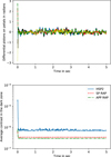 |
Fig. 11 Impact of the petaling on the coronagraphic performance. Top: differential piston sequence in radians over 5 s for five petals, the sixth being the reference, for r0 = 21.5 cm conditions, behind the AO system and combined with continuity hypotheses between petals. Bottom: average contrasts of the three coronagraphs considered in this paper. |
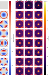 |
Fig. 12 Impact of low-order aberrations on the coronagraphic PSFs. Left: phase maps in radians, from focus to trefoil, each set at 0.25λ RMS except for the first line (no aberration). Right: associated PSFs in logarithmic scale with the three designs, each normalized to its intensity peak. |
Acknowledgements
This project is funded by the European Research Council (ERC) under the European Union's Horizon 2020 research and innovation programme (grant agreement no. 866001 – EXACT). The authors are also grateful to the referee for their pertinent and precise comments that have helped a lot to improve the quality of this paper. All data and codes used in this article are available for free on PerSciDo: Leboulleux (2022).
Appendix A Application to the TMT Aperture
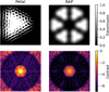 |
Fig. A.1 Amplitude RAP design for the TMT architecture for a single petal (left) and for the full RAP (right). Top: Pupil transmissions from 0 (no transmission) to 1 (full transmission), aiming for a contrast of 10−6 between 8 and 25λ/D; Bottom: Associated PSFs in logarithmic scale. |
The TMT and its 30-meter diameter aperture will have thinner spiders than the ELT (Usuda et al. 2014). However, at bad seeing conditions it might still be subject to island effects that could, for instance, affect the high-contrast performance of the Planetary System Imager (PSI), a proposed second-generation instrument. The RAP concept could then help to mitigate such errors at large angular separations. The aperture used in this appendix is generated by the HCIPy toolkit, which provides AO system and coronagraph simulators (Por et al. 2018) and refers to the description of Jensen-Clem et al. (2021).
The SP RAP design proposed in Fig. A.1 aims for a 10−6 contrast between 8 and 25λ/D and has a 22.3% planetary throughput with a 47.0% transmission. Figure A.2 shows the PSFs with pistons and tip-tilts between the pupil petals for the RAP in Fig. A.1. The amplitudes of the errors were chosen to match the values observed on the SPHERE instrument before the 2017 spider coating. Here the PSFs appear robust to the considered errors.
In Fig. A.3 aberrations with amplitudes between 10 mradian and 10 radians are considered, and for each amplitude 100 random phase maps are simulated and propagated through the coronagraph. For each error amplitude, the average of the 100 mean contrasts is computed and appears on this curve. The RAP design shows a very stable performance for piston-like errors with a plateau at 6.2 × 10⁻⁷ for aberration amplitudes higher than 1 radian RMS and an average contrast in the dark region below 10−6 up to 2.4 radians RMS of petal-level tip-tilt errors.
Since PSI will aim for higher contrasts (~10−8 at 1–2λ/D), a RAP could also be used as a first stage coronagraph. In this case, it could be optimized to reach higher contrasts with a slight loss of robustness at small angular separations.
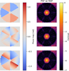 |
Fig. A.2 Robustness to island effect errors between petals in phase maps simulated in the pupil plane in radians (left) and associated PSFs in logarithmic scale with the four designs (right). Three phases are considered: piston only-like errors, at the level observed on SPHERE before coating (top), tip-tilt-only errors, also at the SPHERE level (center), and combined piston-tip-tilt errors from the above rows (bottom). |
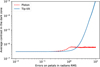 |
Fig. A.3 Evolution of the contrast with island effect errors between petals with piston-like errors (red) and tip-tilt-like errors (blue). For each amplitude error considered here 100 random phase maps are simulated and propagated through the coronagraph, and the average of the 100 contrasts is plotted here. |
References
- Bertrou-Cantou, A., Gendron, E., Rousset, G., et al. 2020, SPIE Conf. Ser., 11448, 1144812 [NASA ADS] [Google Scholar]
- Bertrou-Cantou, A., Gendron, E., Rousset, G., et al. 2022, A&A, 658, A49 [NASA ADS] [CrossRef] [EDP Sciences] [Google Scholar]
- Beuzit, J. L., Vigan, A., Mouillet, D., et al. 2019, A&A, 631, A155 [NASA ADS] [CrossRef] [EDP Sciences] [Google Scholar]
- Boccaletti, A., Chauvin, G., Mouillet, D., et al. 2020, ESO submitted [arXiv:2003.05714] [Google Scholar]
- Bos, S. P., Vievard, S., Wilby, M. J., et al. 2020, A&A, 639, A52 [NASA ADS] [CrossRef] [EDP Sciences] [Google Scholar]
- Brandl, B. R., Absil, O., Agócs, T., et al. 2018, SPIE Conf. Ser., 10702, 107021U [Google Scholar]
- Cantalloube, F., Dohlen, K., Milli, J., Brandner, W., & Vigan, A. 2019, The Messenger, 176, 25 [NASA ADS] [Google Scholar]
- Carlotti, A., Vanderbei, R., & Kasdin, N. J. 2011, Opt. Express, 19, 26796 [NASA ADS] [CrossRef] [Google Scholar]
- Carlotti, A. 2013, A&A, 551, A10 [NASA ADS] [CrossRef] [EDP Sciences] [Google Scholar]
- Carlotti, A., Pueyo, L., & Mawet, D. 2014, A&A, 566, A31 [NASA ADS] [CrossRef] [EDP Sciences] [Google Scholar]
- Carlotti, A., Hénault, F., Dohlen, K., et al. 2018a, SPIE Conf. Ser., 10702, 107029N [NASA ADS] [Google Scholar]
- Carlotti, A., Mouillet, D., Correia, J.-J., et al. 2018b, SPIE Conf. Ser., 10706, 107062M [NASA ADS] [Google Scholar]
- Carlotti, A., Vigan, A., Bonnefoy, M., et al. 2019, in SF2A-2019: Proceedings of the Annual meeting of the French Society of Astronomy and Astrophysics, eds. P. Di Matteo, O. Creevey, A. Crida, G. Kordopatis, J. Malzac, J. B. Marquette, M. N’Diaye, & O. Di Venot [Google Scholar]
- Chilcote, J., Konopacky, Q., De Rosa, R. J., et al. 2020, SPIE Conf. Ser., 11447, 114471S [NASA ADS] [Google Scholar]
- Clénet, Y., Baudoz, P., Davies, R., Tolstoy, E., & Leschinski, K. 2019, in SF2A-2019: Proceedings of the Annual meeting of the French Society of Astronomy and Astrophysics, eds. P. Di Matteo, O. Creevey, A. Crida, G. Kordopatis, J. Malzac, J. B. Marquette, M. N’Diaye, & O. Di Venot [Google Scholar]
- Codona, J. 2007, in In the Spirit of Bernard Lyot: The Direct Detection of Planets and Circumstellar Disks in the 21st Century, 24 [Google Scholar]
- Conan, R., Fusco, T., & Rousset, G. 2005, in Science with Adaptive Optics, eds. W. Brandner, & M. E. Kasper, 97 [CrossRef] [Google Scholar]
- Davies, R., Hörmann, V., Rabien, S., et al. 2021, The Messenger, 182, 17 [NASA ADS] [Google Scholar]
- Ferreira, F., Gratadour, D., Sevin, A., & Doucet, N. 2018a, in 2018 International Conference on High Performance Computing Simulation (HPCS), 180 [Google Scholar]
- Ferreira, F., Gratadour, D., Sevin, A., et al. 2018b, SPIE Conf. Ser., 10703, 1070347 [NASA ADS] [Google Scholar]
- Fogarty, K., Mazoyer, J., St. Laurent, K., et al. 2018, SPIE Conf. Ser., 10698, 106981J [NASA ADS] [Google Scholar]
- Fourer, R., Gay, D., & Kernighan, B. 2002, AMPL: A Modeling Language for Mathematical Programming, 36 [Google Scholar]
- Gerard, B. L., & Marois, C. 2016, SPIE Conf. Ser., 9909, 990958 [Google Scholar]
- Gurobi Optimization, LLC. 2021, Gurobi Optimizer Reference Manual, https://www.gurobi.com [Google Scholar]
- Hénault, F., Carlotti, A., Rabou, P., et al. 2018, SPIE Conf. Ser., 10702, 107028N [Google Scholar]
- Hippler, S., Feldt, M., Bertram, T., et al. 2019, Exp. Astron., 47, 65 [NASA ADS] [CrossRef] [Google Scholar]
- Holzlöhner, R., Kimeswenger, S., Kausch, W., & Noll, S. 2021, A&A, 645, A32 [NASA ADS] [CrossRef] [EDP Sciences] [Google Scholar]
- Houllé, M., Vigan, A., Carlotti, A., et al. 2021, A&A, 652, A67 [NASA ADS] [CrossRef] [EDP Sciences] [Google Scholar]
- Hutterer, V., Shatokhina, I., Obereder, A., & Ramlau, R. 2018, J. Astron. Telescopes Instrum. Syst., 4, 049005 [Google Scholar]
- Jensen-Clem, R., Hinz, P. M., van Kooten, M. A. M., et al. 2021, SPIE Optical Engineering submitted [arXiv:2109.03321] [Google Scholar]
- Jovanovic, N., Martinache, F., Guyon, O., et al. 2015, PASP, 127, 890 [NASA ADS] [CrossRef] [Google Scholar]
- Kasdin, N. J., Vanderbei, R. J., Spergel, D. N., & Littman, M. G. 2003, ApJ, 582, 1147 [NASA ADS] [CrossRef] [Google Scholar]
- Kenworthy, M., Quanz, S., Meyer, M., et al. 2010, The Messenger, 141, 2 [NASA ADS] [Google Scholar]
- Kenworthy, M. A., Absil, O., Agócs, T., et al. 2016, SPIE Conf. Ser., 9908, 9908A6 [NASA ADS] [Google Scholar]
- Korkiakoski, V., Keller, C. U., Doelman, N., et al. 2014, Appl. Opt., 53, 4565 [NASA ADS] [CrossRef] [Google Scholar]
- Lafrenière, D., Marois, C., Doyon, R., & Barman, T. 2009, ApJ, 694, L148 [CrossRef] [Google Scholar]
- Laginja, I., & Leboulleux, L. 2019, zenodo.3382986 [Google Scholar]
- Laginja, I., Soummer, R., Mugnier, L. M., et al. 2021, J. Astron. Telescopes Instrum. Syst., 7, 015004 [NASA ADS] [Google Scholar]
- Laginja, I., Sauvage, J.-F., Mugnier, L. M., et al. 2022, A&A, 658, A84 [NASA ADS] [CrossRef] [EDP Sciences] [Google Scholar]
- Lamb, M., Correia, C., Sauvage, J.-F., et al. 2016, SPIE Conf. Ser., 9909, 99096D [NASA ADS] [Google Scholar]
- Lamb, M. P., Correia, C., Sauvage, J.-F., et al. 2017, J. Astron. Telescopes Instrum. Syst., 3, 039001 [NASA ADS] [CrossRef] [Google Scholar]
- Leboulleux, L. 2022, Redundant Apodized Pupils (RAP) 2 [PerSCiDO dataset] [Google Scholar]
- Leboulleux, L., N’Diaye, M., Riggs, A. J. E., et al. 2016, SPIE Conf. Ser., 9904, 99043C [Google Scholar]
- Leboulleux, L., Sauvage, J.-F., Pueyo, L. A., et al. 2018, J. Astron. Telescopes Instrum. Syst., 4, 035002 [Google Scholar]
- Leboulleux, L., Carlotti, A., & N’Diaye, M. 2022, A&A, 659, A143 [NASA ADS] [CrossRef] [EDP Sciences] [Google Scholar]
- Macintosh, B., Graham, J. R., Barman, T., et al. 2015, Science, 350, 64 [Google Scholar]
- Marois, C., Lafrenière, D., Doyon, R., Macintosh, B., & Nadeau, D. 2006, ApJ, 641, 556 [Google Scholar]
- Martinache, F. 2013, PASP, 125, 422 [NASA ADS] [CrossRef] [Google Scholar]
- Martinez, P., Dorrer, C., Kasper, M., Boccaletti, A., & Dohlen, K. 2010, A&A, 520, A110 [NASA ADS] [CrossRef] [EDP Sciences] [Google Scholar]
- Mazoyer, J., Pueyo, L., N’Diaye, M., et al. 2018a, AJ, 155, 7 [Google Scholar]
- Mazoyer, J., Pueyo, L., N’Diaye, M., et al. 2018b, AJ, 155, 8 [Google Scholar]
- Milli, J., Mouillet, D., Fusco, T., et al. 2017, AO4ELT5 Proceeding, AO4ELT5.0034 [Google Scholar]
- Milli, J., Kasper, M., Bourget, P., et al. 2018, SPIE Conf. Ser., 10703, 107032A [Google Scholar]
- N’Diaye, M., Choquet, E., Pueyo, L., et al. 2013, SPIE Conf. Ser., 8864, 88641K [Google Scholar]
- N’Diaye, M., Choquet, E., Egron, S., et al. 2014, SPIE Conf. Ser., 9143, 914327 [Google Scholar]
- N’Diaye, M., Mazoyer, J., Choquet, É., et al. 2015a, SPIE Conf. Ser., 9605, 96050I [Google Scholar]
- N’Diaye, M., Pueyo, L., & Soummer, R. 2015b, ApJ, 799, 225 [CrossRef] [Google Scholar]
- N’Diaye, M., Vigan, A., Dohlen, K., et al. 2016, A&A, 592, A79 [NASA ADS] [CrossRef] [EDP Sciences] [Google Scholar]
- N’Diaye, M., Martinache, F., Jovanovic, N., et al. 2018, A&A, 610, A18 [Google Scholar]
- Por, E. H. 2017, SPIE Conf. Ser., 10400, 104000V [NASA ADS] [Google Scholar]
- Por, E. H., Haffert, S. Y., Radhakrishnan, V. M., et al. 2018, SPIE Conf. Ser., 10703, 1070342 [NASA ADS] [Google Scholar]
- Por, E. H., Soummer, R., Noss, J., & St. Laurent, K. 2020, SPIE Conf. Ser., 11443, 114433P [Google Scholar]
- Pueyo, L., & Norman, C. 2013, ApJ, 769, 102 [NASA ADS] [CrossRef] [Google Scholar]
- Pueyo, L., Littman, M. G., Carr, M., et al. 2003, SPIE Conf. Ser., 5170, 241 [NASA ADS] [Google Scholar]
- Ruane, G., Riggs, A., Mazoyer, J., et al. 2018, SPIE Conf. Ser., 10698, 106982S [NASA ADS] [Google Scholar]
- Sauvage, J.-F., Fusco, T., Guesalaga, A., et al. 2015, in Adaptive Optics for Extremely Large Telescopes IV (AO4ELT4), E9 [Google Scholar]
- Sauvage, J.-F., Fusco, T., Lamb, M., et al. 2016, SPIE Conf. Ser., 9909, 990916 [Google Scholar]
- Schwartz, N., Sauvage, J.-F., Correia, C., et al. 2018, SPIE Conf. Ser., 10703, 1070322 [NASA ADS] [Google Scholar]
- Soummer, R., Pueyo, L., Ferrari, A., et al. 2009, ApJ, 695, 695 [NASA ADS] [CrossRef] [Google Scholar]
- Soummer, R., Pueyo, L., & Larkin, J. 2012, ApJ, 755, L28 [Google Scholar]
- Soummer, R., Brady, G. R., Brooks, K., et al. 2018, SPIE Conf. Ser., 10698, 106981O [NASA ADS] [Google Scholar]
- Thatte, N., Tecza, M., Schnetler, H., et al. 2021, The Messenger, 182, 7 [NASA ADS] [Google Scholar]
- Usuda, T., Ezaki, Y., Kawaguchi, N., et al. 2014, SPIE Conf. Ser., 9145, 91452F [NASA ADS] [Google Scholar]
- Vanderbei, R. J., Spergel, D. N., & Kasdin, N. J. 2003, ApJ, 590, 593 [NASA ADS] [CrossRef] [Google Scholar]
- Vievard, S., Bos, S., Cassaing, F., et al. 2019, ArXiv e-prints, [arXiv:1912.10179] [Google Scholar]
- Vigan, A., Dohlen, K., N’Diaye, M., et al. 2022, A&A, 660, A140 [NASA ADS] [CrossRef] [EDP Sciences] [Google Scholar]
- Wilby, M. J., Keller, C. U., Sauvage, J. F., et al. 2016, SPIE Conf. Ser., 9909, 99096C [NASA ADS] [Google Scholar]
- Wilby, M. J., Keller, C. U., Sauvage, J. F., et al. 2018, A&A, 615, A34 [NASA ADS] [CrossRef] [EDP Sciences] [Google Scholar]
- Yaitskova, N., & Dohlen, K. 2002, J. Opt. Soc. Am. A, 19, 1274 [NASA ADS] [CrossRef] [Google Scholar]
- Yaitskova, N., Dohlen, K., & Dierickx, P. 2003, J. Opt. Soc. Am. A, 20, 1563 [NASA ADS] [CrossRef] [Google Scholar]
- Zimmerman, N. T., N’Diaye, M., St. Laurent, K. E., et al. 2016, SPIE Conf. Ser., 9904, 99041Y [NASA ADS] [Google Scholar]
All Tables
All Figures
|
Fig. 1 Illustration of the Mickey Mouse effect at a VLT-like configuration (left) Aberration maps applied on the pupil; (right) Associated PSFs in linear scale without aberration (top) and with 415 nm RMS of piston error on the petals (bottom). |
| In the text | |
|
Fig. 2 Low-wind effect on the ELT. (top) Three pupil configurations with the full ELT pupil and the shaped pupils HSP1 and HSP2 of HAR-MONI/HCM, and their associated PSFs in logarithmic scale without low-wind effect (center) and with the low-wind effect phase map of the left column (bottom). The phase map is composed of petal-level pistons, tips, and tilts with average values and variances equivalent to those of VLT/SPHERE before the spider coating (here ~110 nm RMS of piston and ~180 nm RMS of tip and tilt at 1.6 µm). |
| In the text | |
|
Fig. 3 Amplitude apodizations for a single petal (left) and for the full RAP (right). Top: with pupil transmissions from 0 (no transmission) to 1 (full transmission), aiming for a contrast of 10−6 between 8 and 40λ/D. Bottom: associated PSFs in logarithmic scale. |
| In the text | |
|
Fig. 4 Coronagraphic intensity profiles, normalized to the intensity peak, of one of the two shaped pupils designed for the HARMONI configuration (HSP2 in blue), and the two RAPs presented in this paper: the amplitude RAP (red) and the phase RAP (green). The three designs aim for 10−6 contrasts in their dark zones (see Table 1). |
| In the text | |
|
Fig. 5 Phase apodizations for a single petal (left) and for the full RAP (right). Top: pupil phases in radians, aiming for a contrast of 10−6 between 8 and 40λ/D. Bottom: associated PSFs in logarithmic scale. |
| In the text | |
|
Fig. 6 Robustness to low-wind effect errors between petals. Left: phase maps simulated in the pupil plane in radians. Right: associated PSFs in logarithmic scale with the three designs. Four phases are considered (from top to bottom): no error; piston-only errors, at the level observed on SPHERE before coating; tip-tilt-only errors, also at the SPHERE level; combined piston-tip-tilt errors from the above lines. |
| In the text | |
|
Fig. 7 Evolution of the contrast with the piston-like low-wind effect errors between petals with the HSP2 design (blue), the amplitude RAP design (red), and the phase RAP design (green). For each amplitude error considered here, 100 random phase maps are simulated and propagated through the coronagraph, and the average of the 100 contrasts is plotted here. |
| In the text | |
|
Fig. 8 Evolution of the contrast with the tip-tilt-like low-wind effect errors between petals with the HSP2 design (blue), the amplitude RAP design (red), and the phase RAP design (green). For each amplitude error considered here 100 random phase maps are simulated and propagated through the coronagraph, and the average of the 100 contrasts is plotted here. |
| In the text | |
|
Fig. 9 Impact of the petaling on the coronagraphic performance. Top: differential piston sequence in radians over 5 s for five petals, the sixth being the reference, for r0 = 12.8 cm conditions and behind the AO system. Bottom: average contrasts of the three coronagraphs considered in this paper. |
| In the text | |
|
Fig. 10 Impact of the petaling on the coronagraphic performance. Top: Differential piston sequence in radians over 5 s for five petals, the sixth being the reference, for r0 = 12.8 cm conditions, behind the AO system and combined with continuity hypotheses between petals. Bottom: average contrasts of the three coronagraphs considered in this paper. |
| In the text | |
|
Fig. 11 Impact of the petaling on the coronagraphic performance. Top: differential piston sequence in radians over 5 s for five petals, the sixth being the reference, for r0 = 21.5 cm conditions, behind the AO system and combined with continuity hypotheses between petals. Bottom: average contrasts of the three coronagraphs considered in this paper. |
| In the text | |
|
Fig. 12 Impact of low-order aberrations on the coronagraphic PSFs. Left: phase maps in radians, from focus to trefoil, each set at 0.25λ RMS except for the first line (no aberration). Right: associated PSFs in logarithmic scale with the three designs, each normalized to its intensity peak. |
| In the text | |
|
Fig. A.1 Amplitude RAP design for the TMT architecture for a single petal (left) and for the full RAP (right). Top: Pupil transmissions from 0 (no transmission) to 1 (full transmission), aiming for a contrast of 10−6 between 8 and 25λ/D; Bottom: Associated PSFs in logarithmic scale. |
| In the text | |
|
Fig. A.2 Robustness to island effect errors between petals in phase maps simulated in the pupil plane in radians (left) and associated PSFs in logarithmic scale with the four designs (right). Three phases are considered: piston only-like errors, at the level observed on SPHERE before coating (top), tip-tilt-only errors, also at the SPHERE level (center), and combined piston-tip-tilt errors from the above rows (bottom). |
| In the text | |
|
Fig. A.3 Evolution of the contrast with island effect errors between petals with piston-like errors (red) and tip-tilt-like errors (blue). For each amplitude error considered here 100 random phase maps are simulated and propagated through the coronagraph, and the average of the 100 contrasts is plotted here. |
| In the text | |
Current usage metrics show cumulative count of Article Views (full-text article views including HTML views, PDF and ePub downloads, according to the available data) and Abstracts Views on Vision4Press platform.
Data correspond to usage on the plateform after 2015. The current usage metrics is available 48-96 hours after online publication and is updated daily on week days.
Initial download of the metrics may take a while.