| Issue |
A&A
Volume 695, March 2025
|
|
|---|---|---|
| Article Number | A152 | |
| Number of page(s) | 18 | |
| Section | Astrophysical processes | |
| DOI | https://doi.org/10.1051/0004-6361/202452447 | |
| Published online | 14 March 2025 | |
Detection of RS Oph with LST-1 and modelling of its HE/VHE gamma-ray emission
1
Department of Physics, Tokai University, 4-1-1, Kita-Kaname, Hiratsuka, Kanagawa 259-1292, Japan
2
Institute for Cosmic Ray Research, University of Tokyo, 5-1-5, Kashiwa-no-ha, Kashiwa, Chiba 277-8582, Japan
3
INFN and Università degli Studi di Siena, Dipartimento di Scienze Fisiche, della Terra e dell’Ambiente (DSFTA), Sezione di Fisica, Via Roma 56, 53100 Siena, Italy
4
Université Paris-Saclay, Université Paris Cité, CEA, CNRS, AIM, F-91191 Gif-sur-Yvette Cedex, France
5
FSLAC IRL 2009, CNRS/IAC, La Laguna, Tenerife, Spain
6
Departament de Física Quàntica i Astrofísica, Institut de Ciències del Cosmos, Universitat de Barcelona, IEEC-UB, Martí i Franquès, 1, 08028 Barcelona, Spain
7
Instituto de Astrofísica de Andalucía-CSIC, Glorieta de la Astronomía s/n, 18008 Granada, Spain
8
Department of Astronomy, University of Geneva, Chemin d’Ecogia 16, CH-1290 Versoix, Switzerland
9
IPARCOS-UCM, Instituto de Física de Partículas y del Cosmos, and EMFTEL Department, Universidad Complutense de Madrid, Plaza de Ciencias, 1. Ciudad Universitaria, 28040 Madrid, Spain
10
INFN Sezione di Napoli, Via Cintia, ed. G, 80126 Napoli, Italy
11
INAF – Osservatorio Astronomico di Roma, Via di Frascati 33, 00040 Monteporzio Catone, Italy
12
Max-Planck-Institut für Physik, Föhringer Ring 6, 80805 München, Germany
13
INFN Sezione di Padova and Università degli Studi di Padova, Via Marzolo 8, 35131 Padova, Italy
14
Univ. Savoie Mont Blanc, CNRS, Laboratoire d’Annecy de Physique des Particules – IN2P3, 74000 Annecy, France
15
Universität Hamburg, Institut für Experimentalphysik, Luruper Chaussee 149, 22761 Hamburg, Germany
16
Graduate School of Science, University of Tokyo, 7-3-1 Hongo, Bunkyo-ku, Tokyo 113-0033, Japan
17
Faculty of Science and Technology, Universidad del Azuay, Cuenca, Ecuador
18
Centro Brasileiro de Pesquisas Físicas, Rua Xavier Sigaud 150, RJ 22290-180 Rio de Janeiro, Brazil
19
Instituto de Astrofísica de Canarias and Departamento de Astrofísica, Universidad de La Laguna, C. Vía Láctea, s/n, 38205 La Laguna, Santa Cruz de Tenerife, Spain
20
CIEMAT, Avda. Complutense 40, 28040 Madrid, Spain
21
University of Geneva – Département de physique nucléaire et corpusculaire, 24 Quai Ernest Ansernet, 1211 Genève 4, Switzerland
22
INFN Sezione di Bari and Politecnico di Bari, Via Orabona 4, 70124 Bari, Italy
23
Institut de Fisica d’Altes Energies (IFAE), The Barcelona Institute of Science and Technology, Campus UAB, 08193 Bellaterra, (Barcelona), Spain
24
INAF – Osservatorio Astronomico di Brera, Via Brera 28, 20121 Milano, Italy
25
Faculty of Physics and Applied Informatics, University of Lodz, ul. Pomorska 149-153, 90-236 Lodz, Poland
26
INAF – Osservatorio di Astrofisica e Scienza dello spazio di Bologna, Via Piero Gobetti 93/3, 40129 Bologna, Italy
27
Lamarr Institute for Machine Learning and Artificial Intelligence, 44227 Dortmund, Germany
28
INFN Sezione di Trieste and Università degli studi di Udine, Via delle scienze 206, 33100 Udine, Italy
29
INFN Sezione di Catania, Via S. Sofia 64, 95123 Catania, Italy
30
INAF – Istituto di Astrofisica e Planetologia Spaziali (IAPS), Via del Fosso del Cavaliere 100, 00133 Roma, Italy
31
Aix Marseille Univ, CNRS/IN2P3, CPPM, Marseille, France
32
University of Alcalá UAH, Departamento de Physics and Mathematics, Pza. San Diego, 28801 Alcalá de Henares, Madrid, Spain
33
INFN Sezione di Bari and Università di Bari, Via Orabona 4, 70126 Bari, Italy
34
INFN Sezione di Torino, Via P. Giuria 1, 10125 Torino, Italy
35
Dipartimento di Fisica – Universitá degli Studi di Torino, Via Pietro Giuria 1, 10125 Torino, Italy
36
Palacky University Olomouc, Faculty of Science, 17. listopadu 1192/12, 771 46 Olomouc, Czech Republic
37
Dipartimento di Fisica e Chimica “E. Segrè”, Università degli Studi di Palermo, Via Archirafi 36, 90123 Palermo, Italy
38
IRFU, CEA, Université Paris-Saclay, Bât 141, 91191 Gif-sur-Yvette, France
39
Port d’Informació Científica, Edifici D, Carrer de l’Albareda, 08193 Bellaterrra, (Cerdanyola del Vallès), Spain
40
INFN Sezione di Bari, Via Orabona 4, 70125 Bari, Italy
41
Department of Physics, TU Dortmund University, Otto-Hahn-Str. 4, 44227 Dortmund, Germany
42
University of Rijeka, Department of Physics, Radmile Matejcic 2, 51000 Rijeka, Croatia
43
Institute for Theoretical Physics and Astrophysics, Universität Würzburg, Campus Hubland Nord, Emil-Fischer-Str. 31, 97074 Würzburg, Germany
44
Department of Physics and Astronomy, University of Turku, Finland, FI-20014 University of Turku, Finland
45
INFN Sezione di Roma La Sapienza, P.le Aldo Moro, 2, 00185 Rome, Italy
46
ILANCE, CNRS – University of Tokyo International Research Laboratory, University of Tokyo, 5-1-5 Kashiwa-no-Ha Kashiwa City, Chiba 277-8582, Japan
47
Physics Program, Graduate School of Advanced Science and Engineering, Hiroshima University, 1-3-1 Kagamiyama, Higashi-Hiroshima City, Hiroshima 739-8526, Japan
48
INFN Sezione di Roma Tor Vergata, Via della Ricerca Scientifica 1, 00133 Rome, Italy
49
University of Split, FESB, R. Boškovića 32, 21000 Split, Croatia
50
Department of Physics, Yamagata University, 1-4-12 Kojirakawa-machi, Yamagata-shi 990-8560, Japan
51
Institut für Theoretische Physik, Lehrstuhl IV: Plasma-Astroteilchenphysik, Ruhr-Universität Bochum, Universitätsstraße 150, 44801 Bochum, Germany
52
Sendai College, National Institute of Technology, 4-16-1 Ayashi-Chuo, Aoba-ku, Sendai city, Miyagi 989-3128, Japan
53
Josip Juraj Strossmayer University of Osijek, Department of Physics, Trg Ljudevita Gaja 6, 31000 Osijek, Croatia
54
INFN Dipartimento di Scienze Fisiche e Chimiche – Università degli Studi dell’Aquila and Gran Sasso Science Institute, Via Vetoio 1, Viale Crispi 7, 67100 L’Aquila, Italy
55
Chiba University, 1-33, Yayoicho, Inage-ku, Chiba-shi, Chiba 263-8522, Japan
56
Kitashirakawa Oiwakecho, Sakyo Ward, Kyoto 606-8502, Japan
57
FZU – Institute of Physics of the Czech Academy of Sciences, Na Slovance 1999/2, 182 21 Praha 8, Czech Republic
58
Laboratory for High Energy Physics, École Polytechnique Fédérale, CH-1015 Lausanne, Switzerland
59
Astronomical Institute of the Czech Academy of Sciences, Bocni II 1401, 14100 Prague, Czech Republic
60
Faculty of Science, Ibaraki University, 2 Chome-1-1 Bunkyo, Mito, Ibaraki 310-0056, Japan
61
Faculty of Science and Engineering, Waseda University, 3 Chome-4-1 Okubo, Shinjuku City, Tokyo 169-0072, Japan
62
Sorbonne Université, CNRS/IN2P3, Laboratoire de Physique Nucléaire et de Hautes Energies, LPNHE, 4 place Jussieu, 75005 Paris, France
63
Institute of Particle and Nuclear Studies, KEK (High Energy Accelerator Research Organization), 1-1 Oho, Tsukuba 305-0801, Japan
64
INFN Sezione di Trieste and Università degli Studi di Trieste, Via Valerio 2 I, 34127 Trieste, Italy
65
Escuela Politécnica Superior de Jaén, Universidad de Jaén, Campus Las Lagunillas s/n, Edif. A3, 23071 Jaén, Spain
66
Saha Institute of Nuclear Physics, Sector 1, AF Block, Bidhan Nagar, Bidhannagar, Kolkata, West Bengal 700064, India
67
Institute for Nuclear Research and Nuclear Energy, Bulgarian Academy of Sciences, 72 boul. Tsarigradsko chaussee, 1784 Sofia, Bulgaria
68
Dipartimento di Fisica e Astronomia (DIFA) Augusto Righi, Università di Bologna, Via Gobetti 93/2, I-40129 Bologna, Italy
69
Department of Physics and Astronomy, Clemson University, Kinard Lab of Physics, Clemson, SC 29634, USA
70
Dipartimento di Fisica e Chimica ‘E. Segrè’ Università degli Studi di Palermo, Via delle Scienze, 90128 Palermo, Italy
71
Grupo de Electronica, Universidad Complutense de Madrid, Av. Complutense s/n, 28040 Madrid, Spain
72
Institute of Space Sciences (ICE, CSIC), and Institut d’Estudis Espacials de Catalunya (IEEC), and Institució Catalana de Recerca I Estudis Avançats (ICREA), Campus UAB, Carrer de Can Magrans, s/n, 08193 Bellatera, Spain
73
Hiroshima Astrophysical Science Center, Hiroshima University, 1-3-1 Kagamiyama, Higashi-Hiroshima, Hiroshima 739-8526, Japan
74
School of Allied Health Sciences, Kitasato University, Sagamihara, Kanagawa 228-8555, Japan
75
RIKEN, Institute of Physical and Chemical Research, 2-1 Hirosawa, Wako, Saitama 351-0198, Japan
76
Charles University, Institute of Particle and Nuclear Physics, V Holešovičkách 2, 180 00 Prague 8, Czech Republic
77
Division of Physics and Astronomy, Graduate School of Science, Kyoto University, Sakyo-ku, Kyoto 606-8502, Japan
78
Institute for Space-Earth Environmental Research, Nagoya University, Chikusa-ku, Nagoya 464-8601, Japan
79
Kobayashi-Maskawa Institute (KMI) for the Origin of Particles and the Universe, Nagoya University, Chikusa-ku, Nagoya 464-8602, Japan
80
Graduate School of Technology, Industrial and Social Sciences, Tokushima University, 2-1 Minamijosanjima, Tokushima 770-8506, Japan
81
INFN Sezione di Pisa, Edificio C – Polo Fibonacci, Largo Bruno Pontecorvo 3, 56127 Pisa, Italy
82
INFN Dipartimento di Scienze Fisiche e Chimiche – Università degli Studi dell’Aquila and Gran Sasso Science Institute, Via Vetoio 1, Viale Crispi 7, 67100 L’Aquila, Italy
83
Gifu University, Faculty of Engineering, 1-1 Yanagido, Gifu 501-1193, Japan
84
Department of Physical Sciences, Aoyama Gakuin University, Fuchinobe, Sagamihara, Kanagawa 252-5258, Japan
85
Graduate School of Science and Engineering, Saitama University, 255 Simo-Ohkubo, Sakura-ku, Saitama city, Saitama 338-8570, Japan
86
Department of Physics, Konan University, 8-9-1 Okamoto, Higashinada-ku Kobe 658-8501, Japan
⋆ Corresponding authors; lst-contact@cta-observatory.org
Received:
1
October
2024
Accepted:
15
January
2025
Context. The recurrent nova RS Ophiuchi (RS Oph) underwent a thermonuclear eruption in August 2021. In this event, RS Oph was detected by the High Energy Stereoscopic System (H.E.S.S.), the Major Atmospheric Gamma Imaging Cherenkov (MAGIC), and the first Large-Sized Telescope (LST-1) of the future Cherenkov Telescope Array Observatory (CTAO) at very-high gamma-ray energies above 100 GeV. This means that novae are a new class of very-high-energy (VHE) gamma-ray emitters.
Aims. We report the analysis of the RS Oph observations with LST-1. We constrain the particle population that causes the observed emission in hadronic and leptonic scenarios. Additionally, we study the prospects of detecting further novae using LST-1 and the upcoming LST array of CTAO-North.
Methods. We conducted target-of-opportunity observations with LST-1 from the first day of this nova event. The data were analysed in the framework of cta-lstchain and Gammapy, the official CTAO-LST reconstruction and analysis packages. One-zone hadronic and leptonic models were considered to model the gamma-ray emission of RS Oph using the spectral information from Fermi-LAT and LST-1, together with public data from the MAGIC and H.E.S.S. telescopes.
Results. RS Oph was detected at 6.6σ with LST-1 in the first 6.35 hours of observations following the eruption. The hadronic scenario is preferred over the leptonic scenario considering a proton energy spectrum with a power-law model with an exponential cutoff whose position increases from (0.26 ± 0.08) TeV on day 1 up to (1.6 ± 0.6) TeV on day 4 after the eruption. The deep sensitivity and low energy threshold of the LST-1/LST array will allow us to detect faint novae and increase their discovery rate.
Key words: radiation mechanisms: non-thermal / binaries: close / binaries: symbiotic / novae / cataclysmic variables / stars: individual: RS Ophiuchi / gamma rays: stars
© The Authors 2025
 Open Access article, published by EDP Sciences, under the terms of the Creative Commons Attribution License (https://creativecommons.org/licenses/by/4.0), which permits unrestricted use, distribution, and reproduction in any medium, provided the original work is properly cited.
This article is published in open access under the Subscribe to Open model. Subscribe to A&A to support open access publication.
1. Introduction
Novae are thermonuclear runaway explosions on the surface of white dwarfs in binary systems (Chomiuk et al. 2021). Since the addition of novae as a new source class that emits in the high-energy gamma-ray sky (HE; E > 100 MeV; Ackermann et al. 2014), novae have generated interest in the very-high-energy (VHE; E > 100 GeV) gamma-ray domain for their potential to accelerate particles to TeV energies efficiently (e.g., Metzger et al. 2016). Novae also provide an excellent opportunity to study particle acceleration on fast shock-evolution timescales, as well as in abundant systems within the Milky Way (with a Galactic nova rate estimated from different studies between 26–50 yr−1; Zuckerman et al. 2023; Kawash et al. 2022; Rector et al. 2022; De et al. 2021; Shafter 2017). Nevertheless, nova observations did not succeed in a detection at VHE gamma rays (Aliu et al. 2012; Ahnen et al. 2015; Albert et al. 2022) until the 2021 eruption of RS Ophiuchi (RS Oph; H. E. S. S. Collaboration 2022; Acciari et al. 2022).
The source RS Oph is a well-known binary system that experiences recurrent nova explosions that range from 8.6 up to 26.6 years (see Schaefer 2010 for a review). These explosions result from the high mass-accretion rate onto the massive white dwarf driven by the giant companion star. The accretion process in RS Oph is unclear, but the donor star may overfill its Roche lobe (Somero et al. 2017; Schaefer 2009; Booth et al. 2016). RS Oph is characterised as an embedded nova because its eruptions occur immersed in the dense wind of the post-main-sequence companion star (M0 III; Anupama & Mikołajewska 1999). The red giant in these systems produces dense circumbinary material, likely concentrated in the orbital plane. Relativistic particles accelerated via diffusive acceleration in expanding shocks are thought to interact with the dense circumbinary material, generating HE gamma rays (Abdo et al. 2010; Hernanz & Tatischeff 2012; Martin & Dubus 2013).
The first nova detection at HE gamma rays was reported by the Fermi-LAT Collaboration in the symbiotic system V407 Cyg (Abdo et al. 2010). Subsequent nova detections at HE gamma rays from several binary systems and, in particular, those with main-sequence companion stars (known as classical novae; Ackermann et al. 2014), likely indicate that particle acceleration is an intrinsic phenomenon in nova systems (Morris et al. 2016). The detection of classical novae, which do not exhibit a dense circumbinary material, suggests that internal shocks between several outflows can act as another mechanism to accelerate particles in novae (Metzger et al. 2014; Martin et al. 2018; Chomiuk et al. 2021).
Most novae that were detected at HE gamma rays are not embedded in a dense environment. When novae erupt, the detected HE emission presents a similar curved spectral shape regardless of their type (Ackermann et al. 2014). However, the HE luminosity and duration differ and vary depending on the systems (e.g., Ackermann et al. 2014; Cheung et al. 2016; Sokolovsky et al. 2023). Early studies with a limited sample of classical novae suggested an inverse relation between the HE gamma-ray luminosity and its duration (Cheung et al. 2016). However, with a larger sample, this relation may no longer hold. Novae seem to emit for a longer time at HE gamma rays, however, when they take longer to decline from the optical maximum (Albert et al. 2022). Deep gamma-ray observations with multi-wavelength data are required to determine whether the physical differences between the two nova types also reflect a different HE–VHE gamma-ray emission.
During the 2021 nova event of RS Oph, the High Energy Stereoscopic System (H.E.S.S.) and the Major Atmospheric Gamma Imaging Cherenkov (MAGIC) telescope facilities detected RS Oph (H. E. S. S. Collaboration 2022; Acciari et al. 2022). RS Oph is the first nova that was detected at VHE gamma rays and the first confirmation of particle acceleration up to TeV energies in embedded novae. However, the exact acceleration and radiation mechanisms remain unclear, although the favoured explanation for the VHE gamma-ray emission is the hadronic scenario (Martin et al. 2018; Acciari et al. 2022; H. E. S. S. Collaboration 2022; Zheng et al. 2022; Diesing et al. 2023; Sarkar et al. 2023).
The Large-Sized Telescope prototype (LST-1) of the upcoming Cherenkov Telescope Array Observatory (CTAO) observed RS Oph during the nova phase. RS Oph is the first transient source detected with LST-1 during its commissioning phase. In this work, we report the spectral analysis and modelling of RS Oph using LST-1 and Fermi-LAT observations and exploiting published gamma-ray data by H.E.S.S. and MAGIC. In Sect. 2 the observations and the analyses of LST-1 and contemporaneous Fermi-LAT data with LST-1 are described. In Sect. 3 we introduce the model we used to characterise the gamma-ray emission of RS Oph. In Sect. 4 the results from the LST-1 data analysis and the modelling using the Fermi-LAT, LST-1, MAGIC, and H.E.S.S. spectral information are presented. In Sect. 5 we discuss the results and future expectations for nova detections with the array of LSTs of CTAO. Concluding remarks are provided in Sect. 6.
2. Observations and data analysis
In this section, we describe the observation campaign conducted on RS Oph with LST-1 and the analysis procedures we used in this work (Sect. 2.1). We also analyse Fermi-LAT data that were obtained contemporaneously with the LST-1 observations (Sect. 2.2).
2.1. LST-1
The LST is the largest telescope type of the upcoming CTAO. LST-1 is the first out of four LSTs that will constitute the LST array of CTAO in the Northern Hemisphere (CTAO-North; Acharyya et al. 2019). LST-1 is located in the Observatorio del Roque de los Muchachos on the Canary island of La Palma, Spain. Equipped with a 23 m diameter mirror dish, LSTs have a large light-collection area with a camera consisting of high quantum-efficiency photomultiplier tubes. The trigger threshold is optimised to achieve the lowest gamma-ray energy threshold, which is about 20 GeV before the cleaning stage. This makes LSTs ideal telescopes for the observation of gamma-ray sources at energies from tens to hundreds of GeV (Abe et al. 2023a).
LST-1 started follow-up observations of RS Oph based on its detection with Fermi-LAT (Cheung et al. 2021) at HE gamma rays and its bright emission in optical wavelengths. The first LST-1 observation was recorded on August 9 (MJD 59435.90), about one day after the optical trigger. LST-1 observed RS Oph for several days between August 9 and September 2 (MJD 59459.91). In this work, we analyse LST-1 data in good atmospheric1 and dark or low-moonlight observing conditions2 during the observation campaign (see Table 1).
Observation campaign with LST-1.
The LST-1 observations were performed in wobble mode with an offset of 0.4° (Fomin et al. 1994). The LST-1 data were reduced from raw signal waveforms to a list of gamma-like events using the software package cta-lstchain (López-Coto et al. 2022) following the LST-1 standard source-independent analysis approach for the calibration, image cleaning, and parametrisation, gamma-hadron separation, energy and direction reconstruction, and gamma-ray event selection (Abe et al. 2023a). The classification and regression methods rely on random forest algorithms trained on Monte Carlo (MC) gammas and protons, simulated following a declination track of −4.13° in the sky plane, close to the RS Oph declination3. The instrument response functions (IRFs) for each LST-1 observation were produced by interpolating the IRFs calculated at each sky direction of the test MC data to the average telescope pointing direction of each observation. The open-software package Gammapy (Donath et al. 2023; Acero et al. 2022) was used to obtain the scientific products from the gamma-like events, which were assigned based on event selection cuts. For instance, the event angular separation with respect to the source position (θ) and gammaness4 parameters were used in this step. To assess the signal, the same cuts in the whole energy range were used for the above-mentioned parameters. Conversely, the event selection cuts applied to the gamma-like events used to compute the spectral energy distributions (SEDs) and light curve are energy dependent: The cut was set at the value at which 70% of the MC testing gamma rays survive in each energy bin for the θ and gammaness parameters.
We performed a spectral analysis using control sky regions (OFF regions) located around the telescope pointing at the same offset as RS Oph. OFF regions at angular offsets of 90°, 180° and 270° were used, where 0° is towards the telescope pointing and the position of RS Oph. OFF regions were used to subtract the background. The energy threshold of the analysis, computed as the peak position of the energy distribution of the simulated gamma-ray events from a source with a power-law spectral index equal to −4, is E ∼ 30 GeV.
We computed the integral fluxes on a daily basis for observations immediately after the eruption (t − t0 < 4 d, where t0 = MJD 59434.93; Geary 2021) using the spectral shape from the best-fit model for each day. Moreover, we computed integral fluxes by taking several observation days together (hereafter called joint flux; see observation days in Table 1), employing the best-fit spectral model in the corresponding time period. We calculated upper limits (ULs) at the 95% confidence level without considering the systematic uncertainty of the telescope energy scale. The error uncertainties correspond to the 1σ statistical errors.
2.2. Fermi-LAT
The first detection of RS Oph at gamma rays was reported with Fermi-LAT, coincident with the optical discovery (Cheung et al. 2021). The temporal trend in the HE band is similar to the trend in the optical band: A flat peak emission around ∼1 day after the eruption, preceded by a smooth power-law increase and a subsequent power-law decay (slopes between wavelengths consistent within errors). However, the gamma-ray onset was delayed by ∼0.35 day with respect to the time of the eruption and could have reached the peak at later times than in the optical by about 0.5 day (Cheung et al. 2022). The HE gamma-ray emission presents significant spectral curvature, which hardens as the eruption evolves in time. The preferred origin for the HE emission is hadronic, as the model effectively explains the observed emission. No leptonic model was tested in Cheung et al. (2022). We performed a dedicated Fermi-LAT analysis to obtain contemporaneous gamma-ray spectra with the LST-1 observations of RS Oph.
To analyse the Fermi-LAT data, we considered reconstructed events between 50 MeV and 300 GeV with evclass=128 and evtype=3. Only events with good time intervals (DATA_QUAL>0 && LAT_CONFIG==1) coming below a zenith angle of 90° were selected. A binned analysis within a region of interest of 20° around RS Oph was used to model the projected area of interest. We considered in the model all sources in the LAT 10-year source catalogue (4FGL-DR2) together with the Galactic diffuse and the standard isotropic background from Pass 8. All the spectral parameters of all sources within 4° to RS Oph were let free to vary above 50 MeV. No spectral differences were observed when we fixed the spectral parameters of 4FGL J1745.4−0753, the closest source to RS Oph, to its catalogue value. We adopted the latest IRFs (P8R3SOURCEV3) in the analysis. The data processing and analysis were performed using Fermitools version 2.0.8 and Fermipy version 1.0.1 (Fermi Science Support Development Team 2019; Wood et al. 2017).
We extracted the RS Oph daily SED for the days on which LST-1 observed RS Oph. A log-parabola spectral shape was used to model the HE gamma-ray emission (Acciari et al. 2022). The ULs were computed at the 95% confidence level for energy bins with test statistic (TS) values below 4, and the error uncertainties correspond to the 1σ statistical errors. Additionally, when a significant flux was between two ULs, it was set to UL5.
3. Modelling
Proton-proton interactions are thought to be the mechanism for the gamma-ray emission in RS Oph (Acciari et al. 2022; H. E. S. S. Collaboration 2022; Cheung et al. 2022). However, a leptonic contribution to the observed emission cannot be discarded (Sarkar et al. 2023).
We considered the same modelling as was used in Acciari et al. (2022) to model the gamma-ray emission of RS Oph. We considered hadronic and leptonic scenarios to explain its gamma-ray emission. We parametrised the particle spectrum as an exponential cutoff power-law (ECPL) model, while a broken power-law (BPL) model was also considered for the electron spectrum. The same nova parameter values for RS Oph (e.g. distance, ejecta velocity, photosphere radius, and temperature) as were used in Acciari et al. (2022) were assumed in this work (see Table 2) because the data are simultaneous.
Nova parameters used to model the RS Oph gamma-ray SED.
The model maps the ejecta close to a thin layer for the energetic particles. The processes involved in the gamma-ray production for the hadronic scenario are the decay of neutral and charged pions, whereas the inverse-Compton (IC) process alone is considered for the leptonic scenario. Bremsstrahlung emission is negligible because the total column density is lower than the radiation length of hydrogen (Acciari et al. 2022). The seed of photons that dominate during the eruption comes from the photosphere, whose temperature evolves in time (see Table 2). Gamma-gamma absorption is considered in the model. However, it is only relevant for the first day after the eruption (Acciari et al. 2022).
The SED data points at gamma rays from Fermi-LAT, LST-1, MAGIC, and H.E.S.S. were used in the model fitting. As we combine data from multiple instruments, we adapted the model fitting to account for systematic uncertainties in the energy scale of the spectra obtained by the imaging atmospheric Cherenkov telescope (IACT) facilities. A systematic uncertainty in the energy scale between ±15% was considered as a nuisance parameter for each experiment on each day during the fitting process. The absolute 15% maximum value was assumed based on the reported energy-scale uncertainty from MAGIC and H.E.S.S. (Aleksić et al. 2016; H. E. S. S. Collaboration 2022). Similar systematic uncertainties are expected for LST-1 (see Fig. 11 in Abe et al. 2023b). Normally, energy-scale systematics are the dominant effect in IACT. This is especially relevant for soft sources such as RS Oph. However, other types of systematics may contribute, such as uncertainties in the background normalisation, especially at lower energies for a single telescope (Abe et al. 2023a). Including systematic uncertainties in the model fitting reduces the number of degrees of freedom in the fitting process because a displacement of the SED points of the IACTs is allowed with respect to the original points. ULs are not included in the model-fitting minimisation.
The small distance between the LST-1 and MAGIC telescopes means that the measurements with both instruments are not fully independent. Namely, the same gamma-ray shower can be registered by both. The correlation is expected to be energy-dependent and is difficult to evaluate precisely. However, because the trigger rates of both instruments are very different and the source flux was low (i.e. large effect of the random background on the resulting spectra), we expect the correction to be low and therefore treated the two experiments as independent.
4. Results
We report the results of the LST-1 data analysis in Sect. 4.1 and compare them with MAGIC and H.E.S.S. findings. Additionally, the results of the model parameter fitting using Fermi-LAT, LST-1, MAGIC, and H.E.S.S. data are presented in Sect. 4.2, where we also compare the outcomes of the different models.
4.1. LST-1 results
The source RS Oph was detected with LST-1 with a statistical significance of 6.6σ for the three days of LST-1 observations within the first four days from the nova eruption (t − t0 ∼ 1 d, 2 d, and 4 d; see Table 1). The daily statistical significance of the detection is discussed in Appendix A and shown in Table 3. The source was not detected (1.6σ) using the observations conducted three weeks after the nova onset (t − t0 > 21 d).
Best-fit power-law spectral parameter values and statistical detection significances (Sig.) using LST-1 data.
For the purpose of aggregating data from different instruments, we defined observation days as the integer sequence of day intervals centred on t0. The ith observation-day interval spans over MJD t0 + i ± 12 h. The RS Oph daily SEDs at VHE gamma-ray energies with LST-1, including the best-fit spectral models, for the first three observations with LST-1 data on days 1, 2, and 4 after the explosion are shown as blue squares in Fig. 1. A power-law spectral model was adopted to fit the LST-1 data of RS Oph. The spectral index measured with LST-1 is soft for all days and seems to harden as the eruption evolves in time from observation day 1 to observation days 2–4 (see Table 3). However, a spectral profile with a constant index set to the weighted average of the first four observation days cannot be rejected (p−value = 0.11; a significance level6 of α = 0.05 is set to test the null hypothesis). The situation is similar for a constant-amplitude model (p−value = 0.22).
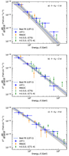 |
Fig. 1. RS Oph daily SEDs at VHE gamma rays with LST-1 (blue squares), MAGIC (orange diamonds; Acciari et al. 2022), and H.E.S.S. (green empty squares and filled circles for the telescopes CT5 and CT1–4, respectively; H. E. S. S. Collaboration 2022) during the same day interval. From top to bottom, panels a, b, and c correspond to observation-day intervals t − t0 ∼ 1 d, 2 d, and 4 d, respectively. The best-fit model for LST-1 is displayed as a blue line together with the grey spectral error band. |
In Fig. 1 we compare the SEDs obtained with LST-1, MAGIC, and H.E.S.S. during the same observation-day intervals (Acciari et al. 2022; H. E. S. S. Collaboration 2022). In general, it is sufficient to only consider statistical errors to obtain compatible results between LST-1 and H.E.S.S./MAGIC, while LST-1 spectra can probe lower energies than the other two IACTs. In addition to the daily SEDs shown in Fig. 1, the joint spectrum for the same observation days (t − t0 ∼ 1 d, 2 d, and 4 d) with LST-1 is provided in Appendix B. The joint LST-1 SED is compatible with that of MAGIC during the same time period.
We show in Fig. 2 the light curve above 100 GeV for LST-1 and MAGIC (Acciari et al. 2022). We show the daily and joint integral fluxes for both instruments. No significant emission is detected with LST-1 above 100 GeV during the first day of data-taking (UL with TS = 2.2). The source flux TS is instead above the UL criterion in the following days, with the LST-1 fluxes values compatible within the statistical uncertainties among them. We obtain less constraining spectral parameter values and a non-significant integral flux for the first observation day than for the second and fourth day because the observation time was shorter and the intrinsic emission was likely softer. The LST-1 daily light curve differs slightly from that of MAGIC when we only consider statistical uncertainties, which suggests the presence of systematics that are not accounted for in the integral flux computation. When the data are joined, however, the joint VHE flux between observation-day intervals 1 and 4 with LST-1 is compatible within the statistical uncertainties with the MAGIC joint integral flux for the same time window. We note that the MAGIC joint flux includes the observations on August 11 (t − t0 ∼ 3 d), when LST-1 did not observe RS Oph. For observations taken at t − t0 > 21 d, when the source was not detected with LST-1, we computed a joint integral flux UL above 100 GeV of 10−11 cm−2 s−1, which was obtained by fixing the power-law spectral index to Γ = −3.5 (the spectral index of observation day 4). The result is comparable in flux level with the MAGIC findings.
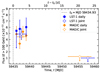 |
Fig. 2. Daily integral fluxes at E > 100 GeV for LST-1 (filled blue squares) and MAGIC (filled orange diamonds; Acciari et al. 2022) as a function of MJD (bottom axis) and time after the eruption onset (top axis), which is represented as the dashed line. We also show the joint LST-1 (empty blue squares) and the joint MAGIC (empty orange diamonds) integral fluxes during observation-day intervals 1 and 4, and more than 21 days after the eruption. |
4.2. Modelling results using Fermi-LAT and IACT data
We show in Fig. 3 the daily SEDs with Fermi-LAT together with the VHE IACT data that were shown in Fig. 1. The gamma-ray spectra span from 50 MeV up to about 1 TeV. The spectral information at HE connects smoothly with that of VHE gamma rays, showing signs of curvature.
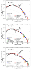 |
Fig. 3. RS Oph daily SEDs from HE to VHE gamma rays using Fermi-LAT (black circles), LST-1 (blue squares), MAGIC (orange diamonds; Acciari et al. 2022), and H.E.S.S. (green empty squares and filled circles for the telescopes CT5 and CT1–4, respectively; H. E. S. S. Collaboration 2022). From top to bottom, panels a, b and c correspond to observation-day intervals t − t0 ∼ 1 d, 2 d, and 4 d, respectively. The best-fit leptonic and hadronic models are displayed as dashed red and solid black curves, respectively. For the hadronic model, the corresponding contributions from neutral and charged-pion decays are shown in grey. |
The emission model was fitted using spectral information from LST-1 and Fermi-LAT data (this work) together with published MAGIC and H.E.S.S. spectral information for each coincident observation-day interval with LST-1. The simplest physically motivated particle energy profile, an ECPL model, without systematic energy-scale uncertainties in the fitting process (see Sect. 3), was considered for the hadronic and leptonic models. The ECPL model is not able to provide a good fit to the data for the leptonic model with reduced χ2 values for each day of about 3 (p−values ∼ 10−5). The poor fit can be explained by the spectral curvature present across the HE and VHE range (as already mentioned by Acciari et al. 2022).
To reproduce the curvature of the gamma-ray spectrum for the leptonic model, we used a BPL shape to describe the energy distribution of electrons, as suggested by Acciari et al. (2022). The fluxes of the best BPL leptonic models are shown as red curves on the daily SEDs in Fig. 3, while the corresponding fit results are displayed in Table 4. The leptonic model with a BPL spectral shape can describe the curvature of the spectrum with Fermi-LAT and IACT data. As the SED evolves with time from observation day 1 to 4, the best-fit parameters of the leptonic model evolve as well: The slope below the energy break softens while the energy break shifts towards higher energies; the slope above the energy break hardens with time. Overall, the electron spectrum reaches higher energies with time. However, the uncertainties of the best-fit parameters of the leptonic model shown in Table 4 are large because the fitting process is rather dependent on the input parameter values (more information on the robustness of the fitting can be found in Appendix C). The spectral parameter results are compatible within the uncertainties with the best-fit leptonic model by Acciari et al. (2022).
Model-fit results without and with systematic uncertainties using the leptonic and hadronic modelling for observation days t − t0 ∼ 1 d, 2 d, and 4 d.
We now consider the ECPL hadronic model to fit the data. The emission of the best model is shown as black curves on the daily SEDs in Fig. 3, while the corresponding fit results are displayed in Table 4. The spectral index softens as the eruption evolves, while the proton spectrum cutoff energy increases with time: from (0.26 ± 0.08) TeV on day 1 to (1.6 ± 0.6) TeV on day 4. A constant cutoff energy during the first three LST-1 observation days is rejected with a p−value = 6 × 10⁻³. The temporal evolution of the proton shape is similar but not compatible within the uncertainties to the one observed with Fermi-LAT and MAGIC alone (Acciari et al. 2022). The hadronic fit of all gamma-ray data presents softer proton spectra and higher cutoff energies.
The Akaike information criterion (AIC) estimator (Akaike 1974) was used to compare different non-nested models. We summed the AIC values corrected for the second-order small-sample bias adjustment (AICc; Hurvich & Tsai 1989) of all observation days for the hadronic and leptonic models (∑AICc, p and ∑AICc, e, respectively) and computed the difference of the higher to the lowest one (∑AICc, min) to compare them (ΔAICc). There is no preference between the hadronic over the leptonic model: ΔAICc = 0.8, which corresponds to a relative likelihood (Akaike 1981) of 0.7, where ∑AICc, min = ∑AICc, e. The slight loss of information, that is, ΔAICc > 0, experienced by using the hadronic over the leptonic model comes from the low χ2 value for the leptonic model on observation day 1. However, on this day, the best-fit leptonic model presents the strongest spectral slope break ( , where Γe, 1 and Γe, 2 are the slope below and above the energy break, respectively). The no-preference of the hadronic model based on the fit statistics disagrees with the results shown in Acciari et al. (2022).
We note that the χred2 for all models deviates from one. Remarkable spectral discrepancies at hundreds of GeV are noticeable between the MAGIC and H.E.S.S. differential fluxes, the latter presenting a harder gamma-ray emission than MAGIC (e.g. see Fig. 1). The mismatch between MAGIC and H.E.S.S. results likely contributes to worsening the goodness of fit of the models. Thus, to account for the LST-1, MAGIC, and H.E.S.S. discrepancies due to possible energy-scale uncertainties in the IACT data analyses, the hadronic and leptonic models were refitted including systematic energy-scale uncertainties as nuisance parameters in the fitting process (see Appendix D). The best-fit results are shown in Table 4. The hadronic and leptonic results with and without systematic are compatible and exhibit the same temporal trends of the particle spectra.
We summed the AICc values of all the observation days and compared the models with and without systematics. The leptonic and hadronic model fits without systematics are both favoured over considering them (ΔAICc = 27.1 and ΔAICc = 20.9, with a relative likelihood of 1 × 10⁻⁶ and 3 × 10⁻⁵ for the leptonic and hadronic models, respectively). Therefore, we discarded the fit results accounting for energy-scale systematics during the model fitting and consider hereafter the leptonic and hadronic model without systematics to describe the relativistic particle energy distribution of RS Oph.
More complicated models can be considered to explain the RS Oph gamma-ray emission. A population of both electrons and protons was used with the lepto-hadronic model in Acciari et al. (2022), even though it was not preferred due to a poor fit and an order of magnitude larger proton-to-electron luminosity ratio (Lp/Le) than the constrained one in the classical nova V339 Del (Acciari et al. 2022). We note that although HE gamma rays are produced in RS Oph and V339 Del, the constrained Lp/Le in the latter may not apply to RS Oph because classical novae such as V339 Del may have different HE particle distribution than embedded novae because the particle acceleration mechanisms and shock formation regions might differ.
The details and results of the lepto-hadronic model are provided in Appendix E. Based on the fit statistics, the lepto-hadronic model is substantially less supported and presents similar parameter values as the hadronic results obtained for observation days t − t0 ∼ 1 d and 4 d, while for the second observation day, the leptonic component dominates the HE band. Therefore, we considered that the lepto-hadronic model is less plausible, based on gamma-ray data alone, to explain the gamma-ray spectrum.
5. Discussion and outlook
The results above show that RS Oph was detected with LST-1 during several coincident days with Fermi-LAT, MAGIC, and H.E.S.S. In this section, we discuss the spectral and modelling results of RS Oph, and we provide an outlook of future expectations for nova detections with the array of LSTs of CTAO.
5.1. Discussion
The data from Fermi-LAT, LST-1, MAGIC, and H.E.S.S. allowed us to study the emission from ∼50 MeV up to multi-TeV energies. This is the largest HE-VHE dataset compiled to date, for which a total exposure time of 6.35 h, 7.7 h, and 9.2 h (6.0 h) is considered for LST-1, MAGIC, and H.E.S.S. CT1–4 (CT5), respectively. While H.E.S.S. constrains the gamma-ray spectrum at about 1 TeV because its sensitivity is better at these energies than that of MAGIC and LST-1, LST-1 bridges the HE and VHE gamma-ray emission and reducing the lower energy bound of the SED of IACTs to ∼30 GeV. This is lower by a factor of ∼2 than the MAGIC energy threshold (Acciari et al. 2022). However, the sensitivity of LST-1 is worse by a factor of ∼1.5 than that of MAGIC above 100 GeV because of the advantages of the stereoscopic reconstruction mode in MAGIC (Abe et al. 2023a).
The model fitting with the Fermi-LAT, LST-1, MAGIC, and H.E.S.S. spectral information describes the spectrum of RS Oph during the first days after the eruption onset using a one-zone single-shock model. Although the hadronic model was slightly preferred statistically over the leptonic model by a combined Fermi-LAT and single IACT data fitting (Acciari et al. 2022), there is no clear preference, based on the fit statistics, between the hadronic and leptonic model using the spectral information from all instruments together.
The simplest ECPL model for the leptonic model cannot adequately describe the curvature of the gamma-ray spectral shape. We also considered the BPL energy distribution shape in the leptonic model to account for this curvature. The physical meaning of using a BPL model is to account for two populations of relativistic electrons as the particles that cause the gamma-ray emission. Therefore, the curvature of the spectrum, which a single population of electrons has difficulties reproducing through IC cooling, is caused by the two populations of relativistic electrons. The leptonic scenario with a BPL model presents several difficulties with respect to the ECPL hadronic model, however. Firstly, our leptonic modelling presents multiple local minima that influence the fitting procedure through the relatively large number of free model parameters. The distribution of the best-fit first slope values (Γe, 1) for observation day 1 is bimodal with two peaks, which complicates the estimation of the confidence interval of this parameter and the χ2 statistics (see Appendix C for details). Secondly, the best-fit electron distributions have a difficult physical interpretation: They are characterised by a very different spectral slope below and above the energy break, as pointed out by Acciari et al. (2022). In particular, the slope break is more pronounced for t − t0 ∼ 1 d, when the emission at HE gamma-rays is bright and the curvature of the spectrum is significantly visible: A flat HE emission is rejected with a p-value of 7 × 10⁻⁵ using the Fermi-LAT SED points presented in this work. A very hard (positive or flat) Γe, 1 index of the electron energy distribution suggests that the fit on the first day tries to imitate the injection of electrons with a high minimum energy (∼14 GeV). The injection of monoenergetic HE particles like these in novae was investigated (in the case of protons) by Bednarek & Śmiałkowski (2022). Nevertheless, on observation day 4, the spectrum below the break is compatible within the uncertainties to the classical −2 slope obtained in diffusive shock acceleration (DSA) for strong shocks (Drury 1983). There is no straightforward explanation for why on this day, a steep ∼−3.5 spectrum also needs to be injected above the break, and why the break energy is comparable (within uncertainties) to the injection energy from the first day of the nova. This picture of the required evolution of the electron energy distribution might be affected by partially cooled-down electrons that were injected at earlier phases. However, as showed by Acciari et al. (2022), the GeV electrons in RS Oph cool down on sub-day time scales. We therefore conclude that while it is possible to describe the gamma-ray observations of RS Oph with a leptonic model, the required injection electron energy distribution is not the one expected from DSA. This disfavours such a model. In consequence, we consider the hadronic scenario to be the most suitable mechanism for explaining the gamma-ray emission.
In the hadronic model, the average total power in protons across the first observation days (t − t0 ∼ 1 d, 2 d and 4 d) is 4.3 × 1043 erg. For a kinetic energy of 2.0 × 1044 erg (Acciari et al. 2022), this indicates that the conversion efficiency of the shock energy to proton energies is about 20%. This considerable amount is aligned with the conversion efficiency estimated by Acciari et al. (2022) and above the lower limit estimated by H. E. S. S. Collaboration (2022).
Systematic uncertainties in the energy scale were introduced in the model fitting to account for systematic errors in the IACT spectral results and reduce their impact on the estimated particle spectrum. However, the model with systematics is less favourable than the model without them, as the addition of three additional free parameters does not significantly improve the goodness of fit. Even though this does not imply that the dataset is free from systematic uncertainties, we chose to discard the model results that accounted for systematics as nuisance parameters. The consistent particle spectra between the hadronic models, both with and without systematics, suggest that the energy-scale uncertainties in the IACT data do not substantially affect the fit results. The primary limitations appear to originate from the small sample size and large flux uncertainties. Additionally, the limited information available from the public data points of MAGIC and H.E.S.S. complicates the application of more refined models that account for upper limits, which provides additional information. While alternative methods might address the systematics between IACTs, these are beyond the scope of this study. Although we discarded the results with systematics, it is worth noting that the sign and time evolution of the best-fit MAGIC and H.E.S.S. systematic energy scaling factors agree with the mismatch between the spectrum from MAGIC and H.E.S.S. and the fact that the gamma-ray emission at VHEs increases in time. This highlights the difference more strongly (see Appendix D).
We consider the best-fit proton spectrum and the subsequent gamma-ray emission from the hadronic modelling without systematics as the reference spectrum for RS Oph. The best-fit proton spectra indicate that protons increase the maximum energy that can reach, up to TeV energies, in agreement with the estimated maximum proton energy and the temporal evolution in the same time period by Cheung et al. (2022), Acciari et al. (2022), H. E. S. S. Collaboration (2022) via DSA. The evolution of the proton spectrum in time is interpreted as the finite acceleration time required for the protons in the expanding shock to accelerate from hundreds of GeV to TeV energies.
Other approaches were used to reproduce the spectral and temporal features observed in the RS Oph eruption: a multi-population particle scenario of electrons and protons (Acciari et al. 2022; Sarkar et al. 2023), or a multi-shock scenario approach (Diesing et al. 2023).
On the one hand, related to the multi-population particle scenario of electrons and protons, the non-thermal radio detection at early times supports the presence of relativistic electrons that rise early during the eruption for both classical and embedded novae (e.g., Chomiuk et al. 2014; Finzell et al. 2018; Weston et al. 2016; O’Brien et al. 2006; Molina et al. 2024). In particular, non-thermal radio emission has been detected coincident with HE gamma rays in embedded ones (Linford et al. 2017; de Ruiter et al. 2023; Nyamai et al. 2023). For instance, synchrotron emission was detected coincident in time with the gamma-ray emission in RS Oph (de Ruiter et al. 2023) and the gamma-ray nova candidate V1535 Sco (Linford et al. 2017; Franckowiak et al. 2018). However, the gamma-ray contribution from IC losses at early times is unclear. A detailed multi-frequency follow-up monitoring is required to obtain a precise spectrum to constrain the physics that cause the broad non-thermal emission. When the lepto-hadronic model in Acciari et al. (2022) was fitted with all available gamma-ray data, the HE component was described by IC, but with a hard spectral index, and it was disfavoured with respect to the leptonic and the hadronic models by the fit statistics. This may imply that there are further components within the very early gamma-ray emission from recurrent nova. This goes beyond the scope of this study, however, and requires early multi-wavelength observations of nova and additional modelling.
On the other hand, connected to the multi-shock scenario, the non-spherical ejecta observed in RS Oph and expected in embedded novae driven by the secondary star (Munari et al. 2022; Booth et al. 2016; Orlando et al. 2017; Islam et al. 2024), the multiple velocity components in the 2021 RS Oph nova (Diesing et al. 2023), and a possible localised shock-acceleration event (Cheung et al. 2022) support the idea of a system with multiple shocks that evolve during the eruption. However, a single hadronic population model with spherical symmetry can reproduce the observed spectrum and temporal evolution at HE and VHE gamma-ray energies with acceptable accuracy (see Table 4). Furthermore, the temporal evolution of the proton energy distribution seems reasonably explained by the finite acceleration time for particles to reach TeV energies. To shed light on this matter, the observation of future bright novae with detectors with better sensitivities and deeper monitoring campaigns could help distinguish between the acceleration mechanisms and the contribution of non-thermal emission from a multiple particle population scenario (single or multiple shocks in a hadronic or lepton-hadronic scenario).
5.2. Outlook
The source RS Oph belongs to a specific nova class in which a binary system with a giant donor companion star undergoes recurrent outbursts. This class contains a few members: T CrB, V3890 Sgr, V745 Sco, and RS Oph (Bode & Evans 2012). T CrB is the closest system to Earth from this class (∼ 0.9 kpc; Gaia Collaboration 2023), followed by RS Oph. T CrB is expected to erupt again in the mid-2020s (Schaefer 2023; Schaefer et al. 2023; Luna et al. 2020). When we assume that T CrB will manifest the same spectral profile as RS Oph, T CrB will likely present a brighter flux than RS Oph by a factor of ∼7, making T CrB one of the brightest novae at gamma rays up to date. In Fig. 4, the best-fit SED models of seven embedded (V407 Cyg, T CrB, and RS Oph) and classical (V906 Car, V959 Mon, V1324 Sco, and V339 Del) novae detected at HE gamma rays are displayed together with the tentative gamma-ray SED from T CrB based on the RS Oph spectral shape on day 1, with the flux amplitude scaled to account for the difference in distance between them. The observed SED for the different novae is diverse, possibly due to their intrinsic nature and/or distance. Moreover, the observed SED models were estimated considering different observation time spans depending on the duration of the gamma-ray detection7. Between 17 and 27 days of data were used to produce the gamma-ray spectral models in Fig. 4 (except RS Oph; Aydi et al. 2020; Ackermann et al. 2014). Hence, the displayed gamma-ray spectrum cannot accurately describe the maximum flux level or any spectral variability during the nova events. In addition, the gamma-ray flux for the Fermi-LAT novae was extrapolated to the CTAO energy range assuming the best-fit spectral shape reported with Fermi-LAT, consisting of an ECPL for the first novae detected with Fermi-LAT. In contrast, a log-parabola model was considered for V906 Car, which resembles the RS Oph spectral shape, but has a lower flux. The expected bright gamma-ray flux of T CrB should help us to constrain the parameters of the particle population that causes the gamma-ray emission in novae even better.
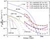 |
Fig. 4. Best-fit SED models for RS Oph (black; this work, t − t0 ∼ 1 d), V906 Car (grey; Aydi et al. 2020), the first novae detected with Fermi-LAT (V407 Cyg, orange; V1324 Sco, green; V959 Mon, brown; V339 Del, pink; Ackermann et al. 2014), and the expected SED from T CrB (blue). The solid region of the nova SEDs approximately corresponds to the energy range where the model was fitted to the data, while the spaced-dashed region corresponds to the extrapolation region of the model. In addition, the sensitivity curves for LST-1 at low zenith angles (zd < 35 °; red square curves; Abe et al. 2023a) and the four LSTs of CTAO-North at zd = 20° (purple circle curves; using the latest Prod5-v0.1 IRFs in Cherenkov Telescope Array Observatory & Cherenkov Telescope Array Consortium 2021) for 5 and 50 hours of observation time (see text for details) are displayed as solid and dotted curves, respectively. |
It is still an open question whether classical novae can emit VHE gamma rays or if a bright VHE gamma-ray emission requires a similar binary system configuration as RS Oph, a recurrent nova embedded in the red giant star envelope. Related to the former, the brightest classical nova detected at HE gamma rays so far is V906 Car (Aydi et al. 2020). Its best-fit SED model is displayed in Fig. 4 together with the detection sensitivity curves for LST-1 and the array of four LSTs of CTAO-North for an integration time of 5 h and 50 h. The standard definition of sensitivity is used: The minimum flux for a 5σ detection, with a requirement of a signal-to-background ratio of 5% at least. This definition only applies to point-like sources calculated in a five-bins per decade logarithmic energy binning. In particular, the sensitivity curves for LST-1 correspond to the average performance below 35° zenith angle (Abe et al. 2023a), while the LST array sensitivity curves are computed at 20°. Specifically, the IRFs at 20° in zenith and average azimuth. Different novae will be observed with LSTs and will culminate at different zenith angles. Hence, some of them may not be observable at this low zenith angle, implying that the sensitivity at low energies that can be achieved in these observations will degrade. When we compares the sensitivity curves for one and four LSTs, the latter will outperform the former by an order of magnitude at energies below 100 GeV. This improvement is due to the larger collection area and background rejection by the stereo-trigger method. Figure 4 shows that the V906 Car SED model remains below the sensitivity curve of LST-1 even for 50 hours of integrated time. Nonetheless, when the CTAO will be operational and the four LSTs dominate the sensitivity of CTAO in the low-energy range, the possibility of detecting fainter novae than RS Oph will grow. The LST array sensitivity for 50 h reaches a flux level similar to the model emission of V906 Car at tens of GeV. This observation time can be challenging to achieve in fast eruptions, but a detection with a shorter integration time may be possible for closer novae than V906 Car. Furthermore, since the nova SED models in Fig. 4 are time averaged (except RS Oph), the nova spectral models underestimate the emission level in the peak of the gamma-ray phase, when a detection is most probable.
We note, however, that the emission models in Fig. 4 highly depend on the assumption that the observed spectral shape at HE gamma rays is constrained enough and can be extrapolated to the VHE gamma-ray band. At HE gamma rays, the spectral curvature for most novae is better described by an ECPL shape with cutoff photon energies at a few GeV (e.g., Ackermann et al. 2014; Cheung et al. 2016). Nevertheless, the emissions of RS Oph and V906 Car, the brightest embedded and classical novae, are better explained by a log-parabola shape (Acciari et al. 2022; H. E. S. S. Collaboration 2022; Aydi et al. 2020). Acciari et al. (2022) suggested that the spectral shape of RS Oph is not different from other novae, but its bright emission is the cause of the VHE gamma-ray detection. The expected TeV emission in the case of V407 Cyg and V339 Del for an RS Oph-like spectrum would be below the reported UL constraints (Acciari et al. 2022). Under this assumption, the extrapolated emission for the ECPL model for HE novae will underestimate the emission of an RS-Oph-like shape at VHE gamma rays.
Moreover, the VHE emission will depend on the properties of the system and the ejecta if the observed cutoff energy in the photon spectrum of all novae originates from the balance between acceleration and cooling processes. In this regard, Cherenkov Telescope Array Consortium (2024) explored the capabilities of CTAO to constrain the physical parameters of novae from a modelling and parameter study approach, assuming that the VHE gamma rays are produced through hadronic interactions. The novae detectability and extension in time would depend on the shock velocity and ejecta mass. Furthermore, the parameter space study showed that 30% of the brightest sample would be detectable with CTAO. These constraints on the VHE emission with multi-wavelength observations will be relevant for constraining the physical parameters of the nova phenomena and for determining whether the physical differences in embedded and classical nova systems also reflect in their gamma-ray emission.
6. Conclusions
The source RS Oph is the first nova that was detected at VHE gamma rays and the first transient source that was detected with the first LST of the future CTAO. During the first observation days after the eruption (t − t0 ∼ 1 d, 2 d, and 4 d), RS Oph was statistically detected at 6.6σ with LST-1 and was characterised by a soft power-law emission at energies E = [0.03, 1] TeV. LST-1 spectral results are consistent with the emission reported with MAGIC and H.E.S.S. in coincident observation-day intervals with LST-1. We did not detect RS Oph with LST-1 after 21 days after the eruption onset.
We obtained the particle energy spectrum during the LST-1 observations immediately after the eruption onset by using the most complete gamma-ray spectrum to date, including Fermi-LAT, LST-1, H.E.S.S., and MAGIC spectral information. The simpler spectral shape of the hadronic model supports the hadronic over the leptonic scenario to explain the RS Oph gamma-ray emission, although the relative likelihood of the two models is comparable. The proton energy spectrum evolves with time, increasing the maximum energy of the accelerated protons from hundreds of GeV up to TeV energies between observation-day intervals 1 and 4 after the eruption. The results were validated with a set of robustness tests (Appendix C).
In the following years, other novae can be expected to be detectable by IACTs. The next eruption of T CrB is foreseen to occur and likely become a bright nova at gamma-ray energies. An event like this is expected to give outstanding constraints in the evolution of gamma-ray emission during the eruption phase and the maximum energy attainable by the accelerated particles in embedded novae. In the near future, the better sensitivity of the LST array with respect to current facilities at low energies will allow us to probe fainter gamma-ray fluxes. A better sensitivity may enable the detection of classical novae, a nova type yet to be detected at VHE gamma rays.
Acknowledgments
We thank the anonymous referee for useful suggestions and comments that helped to improve the content of the manuscript. We gratefully acknowledge financial support from the following agencies and organisations: Conselho Nacional de Desenvolvimento Científico e Tecnológico (CNPq), Fundação de Amparo à Pesquisa do Estado do Rio de Janeiro (FAPERJ), Fundação de Amparo à Pesquisa do Estado de São Paulo (FAPESP), Fundação de Apoio à Ciência, Tecnologia e Inovação do Paraná – Fundação Araucária, Ministry of Science, Technology, Innovations and Communications (MCTIC), Brasil; Ministry of Education and Science, National RI Roadmap Project DO1-153/28.08.2018, Bulgaria; Croatian Science Foundation, Rudjer Boskovic Institute, University of Osijek, University of Rijeka, University of Split, Faculty of Electrical Engineering, Mechanical Engineering and Naval Architecture, University of Zagreb, Faculty of Electrical Engineering and Computing, Croatia; Ministry of Education, Youth and Sports, MEYS LM2023047, EU/MEYS CZ.02.1.01/0.0/0.0/16_013/0001403, CZ.02.1.01/0.0/0.0/18_046/0016007, CZ.02.1.01/0.0/0.0/16_019/0000754, CZ.02.01.01/00/22_008/0004632 and CZ.02.01.01/00/23_015/0008197 Czech Republic; CNRS-IN2P3, the French Programme d’investissements d’avenir and the Enigmass Labex, This work has been done thanks to the facilities offered by the Univ. Savoie Mont Blanc – CNRS/IN2P3 MUST computing center, France; Max Planck Society, German Bundesministerium für Bildung und Forschung (Verbundforschung / ErUM), Deutsche Forschungsgemeinschaft (SFBs 876 and 1491), Germany; Istituto Nazionale di Astrofisica (INAF), Istituto Nazionale di Fisica Nucleare (INFN), Italian Ministry for University and Research (MUR), and the financial support from the European Union – Next Generation EU under the project IR0000012 – CTA+ (CUP C53C22000430006), announcement N.3264 on 28/12/2021: “Rafforzamento e creazione di IR nell’ambito del Piano Nazionale di Ripresa e Resilienza (PNRR)”; ICRR, University of Tokyo, JSPS, MEXT, Japan; JST SPRING – JPMJSP2108; Narodowe Centrum Nauki, grant number 2019/34/E/ST9/00224, Poland; The Spanish groups acknowledge the Spanish Ministry of Science and Innovation and the Spanish Research State Agency (AEI) through the government budget lines PGE2021/28.06.000X.411.01, PGE2022/28.06.000X.411.01 and PGE2022/28.06.000X.711.04, and grants PID2022-139117NB-C44, PID2019-104114RB-C31, PID2019-107847RB-C44, PID2019-104114RB-C32, PID2019-105510GB-C31, PID2019-104114RB-C33, PID2019-107847RB-C41, PID2019-107847RB-C43, PID2019-107847RB-C42, PID2019-107988GB-C22, PID2021-124581OB-I00, PID2021-125331NB-I00, PID2022-136828NB-C41, PID2022-137810NB-C22, PID2022-138172NB-C41, PID2022-138172NB-C42, PID2022-138172NB-C43, PID2022-139117NB-C41, PID2022-139117NB-C42, PID2022-139117NB-C43, PID2022-139117NB-C44, PID2022-136828NB-C42 funded by the Spanish MCIN/AEI/ 10.13039/501100011033 and “ERDF A way of making Europe; the “Centro de Excelencia Severo Ochoa” program through grants no. CEX2019-000920-S, CEX2020-001007-S, CEX2021-001131-S; the “Unidad de Excelencia María de Maeztu” program through grants no. CEX2019-000918-M, CEX2020-001058-M; the “Ramón y Cajal” program through grants RYC2021-032991-I funded by MICIN/AEI/10.13039/501100011033 and the European Union “NextGenerationEU”/PRTR; RYC2021-032552-I and RYC2020-028639-I; the “Juan de la Cierva-Incorporación” program through grant no. IJC2019-040315-I and “Juan de la Cierva-formación”’ through grant JDC2022-049705-I. They also acknowledge the “Atracción de Talento” program of Comunidad de Madrid through grant no. 2019-T2/TIC-12900; the project “Tecnologiás avanzadas para la exploracioń del universo y sus componentes” (PR47/21 TAU), funded by Comunidad de Madrid, by the Recovery, Transformation and Resilience Plan from the Spanish State, and by NextGenerationEU from the European Union through the Recovery and Resilience Facility; the La Caixa Banking Foundation, grant no. LCF/BQ/PI21/11830030; Junta de Andalucía under Plan Complementario de I+D+I (Ref. AST22_0001) and Plan Andaluz de Investigación, Desarrollo e Innovación as research group FQM-322; “Programa Operativo de Crecimiento Inteligente” FEDER 2014-2020 (Ref. ESFRI-2017-IAC-12), Ministerio de Ciencia e Innovación, 15% co-financed by Consejería de Economía, Industria, Comercio y Conocimiento del Gobierno de Canarias; the “CERCA” program and the grants 2021SGR00426 and 2021SGR00679, all funded by the Generalitat de Catalunya; and the European Union’s “Horizon 2020” GA:824064 and NextGenerationEU (PRTR-C17.I1). This research used the computing and storage resources provided by the Port d’Informació Científica (PIC) data center. State Secretariat for Education, Research and Innovation (SERI) and Swiss National Science Foundation (SNSF), Switzerland; The research leading to these results has received funding from the European Union’s Seventh Framework Programme (FP7/2007-2013) under grant agreements No 262053 and No 317446; This project is receiving funding from the European Union’s Horizon 2020 research and innovation programs under agreement No 676134; ESCAPE – The European Science Cluster of Astronomy & Particle Physics ESFRI Research Infrastructures has received funding from the European Union’s Horizon 2020 research and innovation programme under Grant Agreement no. 824064. This work was conducted in the context of the CTA Consortium. This paper has gone through internal review by the CTA Consortium. Author contribution: A. Aguasca-Cabot: project coordination, LST-1 data analysis, model fitting, paper drafting and edition; M. I. Bernardos: Fermi-LAT and LST-1 data analysis; P. Bordas: discussion of model fitting and results; D. Green: project coordination; Y. Kobayashi: LST-1 data analysis; R. López-Coto: project coordination; M. Ribó: discussion of model fitting and results; J. Sitarek: model-fitting codes and edition of the discussion section. All these authors have participated in the paper drafting. The rest of the authors have contributed in one or several of the following ways: design, construction, maintenance and operation of the instrument(s) used to acquire the data; preparation and/or evaluation of the observation proposals; data acquisition, processing, calibration and/or reduction; production of analysis tools and/or related Monte Carlo simulations; discussion and approval of the contents of the draft.
References
- Abdo, A. A., Ackermann, M., Ajello, M., et al. 2010, Science, 329, 817 [NASA ADS] [CrossRef] [Google Scholar]
- Abe, H., Abe, K., Abe, S., et al. 2023a, ApJ, 956, 80 [CrossRef] [Google Scholar]
- Abe, H., Abe, K., Abe, S., et al. 2023b, A&A, 680, A66 [CrossRef] [EDP Sciences] [Google Scholar]
- Acciari, V. A., Ansoldi, S., Antonelli, L. A., et al. 2022, Nat. Astron., 6, 689 [NASA ADS] [CrossRef] [Google Scholar]
- Acero, F., Aguasca-Cabot, A., Buchner, J., et al. 2022, https://doi.org/10.5281/zenodo.7311399 [Google Scholar]
- Acharyya, A., Agudo, I., Angüner, E. O., et al. 2019, Astropart. Phys., 111, 35 [NASA ADS] [CrossRef] [Google Scholar]
- Ackermann, M., Ajello, M., Albert, A., et al. 2014, Science, 345, 554 [NASA ADS] [CrossRef] [Google Scholar]
- Ahnen, M. L., Ansoldi, S., Antonelli, L. A., et al. 2015, A&A, 582, A67 [NASA ADS] [CrossRef] [EDP Sciences] [Google Scholar]
- Akaike, H. 1974, IEEE Trans. Autom. Control, 19, 716 [Google Scholar]
- Akaike, H. 1981, J. Econom., 16, 3 [CrossRef] [Google Scholar]
- Albert, A., Alfaro, R., Alvarez, C., et al. 2022, ApJ, 940, 141 [NASA ADS] [CrossRef] [Google Scholar]
- Aleksić, J., Ansoldi, S., Antonelli, L., et al. 2016, Astropart. Phys., 72, 76 [NASA ADS] [CrossRef] [Google Scholar]
- Aliu, E., Archambault, S., Arlen, T., et al. 2012, ApJ, 754, 77 [NASA ADS] [CrossRef] [Google Scholar]
- Anupama, G. C., & Mikołajewska, J. 1999, A&A, 344, 177 [NASA ADS] [Google Scholar]
- Aydi, E., Sokolovsky, K. V., Chomiuk, L., et al. 2020, Nat. Astron., 4, 776 [CrossRef] [Google Scholar]
- Bednarek, W., & Śmiałkowski, A. 2022, MNRAS, 511, 3339 [NASA ADS] [CrossRef] [Google Scholar]
- Bode, M. F., & Evans, A. 2012, Classical Novae (Cambridge, UK: Cambridge University Press) [Google Scholar]
- Booth, R. A., Mohamed, S., & Podsiadlowski, P. 2016, MNRAS, 457, 822 [NASA ADS] [CrossRef] [Google Scholar]
- Cherenkov Telescope Array Consortium 2024, Science with the Cherenkov Telescope Array (World Scientific Publishing Co. Pte. Ltd.) [Google Scholar]
- Cherenkov Telescope Array Observatory& Cherenkov Telescope Array Consortium 2021, https://doi.org/10.5281/zenodo.5499840 [Google Scholar]
- Cheung, C. C., Jean, P., Shore, S. N., et al. 2016, ApJ, 826, 142 [NASA ADS] [CrossRef] [Google Scholar]
- Cheung, C. C., Ciprini, S., & Johnson, T. J. 2021, ATel, 14834, 1 [NASA ADS] [Google Scholar]
- Cheung, C. C., Johnson, T. J., Jean, P., et al. 2022, ApJ, 935, 44 [NASA ADS] [CrossRef] [Google Scholar]
- Chomiuk, L., Linford, J. D., Yang, J., et al. 2014, Nature, 514, 339 [NASA ADS] [CrossRef] [Google Scholar]
- Chomiuk, L., Metzger, B. D., & Shen, K. J. 2021, ARA&A, 59, 391 [NASA ADS] [CrossRef] [Google Scholar]
- De, K., Kasliwal, M. M., Hankins, M. J., et al. 2021, ApJ, 912, 19 [NASA ADS] [CrossRef] [Google Scholar]
- de Ruiter, I., Nyamai, M. M., Rowlinson, A., et al. 2023, MNRAS, 523, 132 [NASA ADS] [CrossRef] [Google Scholar]
- Diesing, R., Metzger, B. D., Aydi, E., et al. 2023, ApJ, 947, 70 [NASA ADS] [CrossRef] [Google Scholar]
- Donath, A., Terrier, R., Remy, Q., et al. 2023, A&A, 678, A157 [NASA ADS] [CrossRef] [EDP Sciences] [Google Scholar]
- Drury, L. O. 1983, Rep. Progr. Phys., 46, 973 [Google Scholar]
- Fermi Science Support Development Team. 2019, Astrophysics Source Code Library [record ascl:1905.011] [Google Scholar]
- Finzell, T., Chomiuk, L., Metzger, B. D., et al. 2018, ApJ, 852, 108 [NASA ADS] [CrossRef] [Google Scholar]
- Fomin, V., Stepanian, A., Lamb, R., et al. 1994, Astropart. Phys., 2, 137 [NASA ADS] [CrossRef] [Google Scholar]
- Franckowiak, A., Jean, P., Wood, M., Cheung, C. C., & Buson, S. 2018, A&A, 609, A120 [NASA ADS] [CrossRef] [EDP Sciences] [Google Scholar]
- Gaia Collaboration (Vallenari, A., et al.) 2023, A&A, 674, A1 [NASA ADS] [CrossRef] [EDP Sciences] [Google Scholar]
- Geary, K. 2021, VSNET-alert, 26131, 1 [Google Scholar]
- H. E. S. S. Collaboration (Aharonian, F., et al.) 2022, Science, 376, 77 [NASA ADS] [CrossRef] [Google Scholar]
- Hernanz, M., & Tatischeff, V. 2012, Balt. Astron., 21, 62 [NASA ADS] [Google Scholar]
- Hurvich, C. M., & Tsai, C.-L. 1989, Biometrika, 76, 297 [CrossRef] [Google Scholar]
- Islam, N., Mukai, K., & Sokoloski, J. L. 2024, ApJ, 960, 125 [NASA ADS] [CrossRef] [Google Scholar]
- Kawash, A., Chomiuk, L., Strader, J., et al. 2022, ApJ, 937, 64 [NASA ADS] [CrossRef] [Google Scholar]
- Li, T. P., & Ma, Y. Q. 1983, ApJ, 272, 317 [CrossRef] [Google Scholar]
- Linford, J. D., Chomiuk, L., Nelson, T., et al. 2017, ApJ, 842, 73 [NASA ADS] [CrossRef] [Google Scholar]
- López-Coto, R., Baquero, A., Bernardos, M. I., et al. 2022, ASP Conf. Ser., 532, 357 [Google Scholar]
- Luna, G. J. M., Sokoloski, J. L., Mukai, K., & Kuin, N. P. M. 2020, ApJ, 902, L14 [NASA ADS] [CrossRef] [Google Scholar]
- Martin, P., & Dubus, G. 2013, A&A, 551, A37 [NASA ADS] [CrossRef] [EDP Sciences] [Google Scholar]
- Martin, P., Dubus, G., Jean, P., Tatischeff, V., & Dosne, C. 2018, A&A, 612, A38 [NASA ADS] [CrossRef] [EDP Sciences] [Google Scholar]
- Metzger, B. D., Hascoët, R., Vurm, I., et al. 2014, MNRAS, 442, 713 [NASA ADS] [CrossRef] [Google Scholar]
- Metzger, B. D., Caprioli, D., Vurm, I., et al. 2016, MNRAS, 457, 1786 [NASA ADS] [CrossRef] [Google Scholar]
- Molina, I., Chomiuk, L., Linford, J. D., et al. 2024, MNRAS, 534, 1227 [CrossRef] [Google Scholar]
- Morris, P. J., Cotter, G., Brown, A. M., & Chadwick, P. M. 2016, MNRAS, 465, 1218 [Google Scholar]
- Munari, U., Giroletti, M., Marcote, B., et al. 2022, A&A, 666, L6 [NASA ADS] [CrossRef] [EDP Sciences] [Google Scholar]
- Nyamai, M. M., Linford, J. D., Allison, J. R., et al. 2023, MNRAS, 523, 1661 [NASA ADS] [CrossRef] [Google Scholar]
- O’Brien, T. J., Bode, M. F., Porcas, R. W., et al. 2006, Nature, 442, 279 [CrossRef] [Google Scholar]
- Orlando, S., Drake, J. J., & Miceli, M. 2017, MNRAS, 464, 5003 [CrossRef] [Google Scholar]
- Rector, T. A., Shafter, A. W., Burris, W. A., et al. 2022, ApJ, 936, 117 [NASA ADS] [CrossRef] [Google Scholar]
- Sarkar, A. D., Nayana, A. J., Roy, N., Razzaque, S., & Anupama, G. C. 2023, ApJ, 951, 62 [NASA ADS] [CrossRef] [Google Scholar]
- Schaefer, B. E. 2009, ApJ, 697, 721 [NASA ADS] [CrossRef] [Google Scholar]
- Schaefer, B. E. 2010, ApJS, 187, 275 [NASA ADS] [CrossRef] [Google Scholar]
- Schaefer, B. E. 2023, MNRAS, 524, 3146 [NASA ADS] [CrossRef] [Google Scholar]
- Schaefer, B. E., Kloppenborg, B., Waagen, E. O., & Observers, T. A. 2023, ATel, 16107, 1 [NASA ADS] [Google Scholar]
- Shafter, A. W. 2017, ApJ, 834, 196 [CrossRef] [Google Scholar]
- Sokolovsky, K. V., Johnson, T. J., Buson, S., et al. 2023, MNRAS, 521, 5453 [NASA ADS] [CrossRef] [Google Scholar]
- Somero, A., Hakala, P., & Wynn, G. A. 2017, MNRAS, 464, 2784 [NASA ADS] [CrossRef] [Google Scholar]
- Weston, J. H. S., Sokoloski, J. L., Metzger, B. D., et al. 2016, MNRAS, 457, 887 [NASA ADS] [CrossRef] [Google Scholar]
- Wood, M., Caputo, R., Charles, E., et al. 2017, in 35th International Cosmic Ray Conference (ICRC2017), Int. Cosmic Ray Conf., 301, 824 [Google Scholar]
- Zheng, J.-H., Huang, Y.-Y., Zhang, Z.-L., et al. 2022, Phys. Rev. D, 106, 103011 [NASA ADS] [CrossRef] [Google Scholar]
- Zuckerman, L., De, K., Eilers, A.-C., Meisner, A. M., & Panagiotou, C. 2023, MNRAS, 523, 3555 [NASA ADS] [CrossRef] [Google Scholar]
Appendix A: Daily statistical detection significance
The statistical detection significance (formula 17; Li & Ma 1983) for the full energy range on each day is 3.2σ, 2.8σ and 5.5σ for t − t0 = 1 d, 2 d and 4 d, respectively. We note that the event selection cuts used to compute the detection significance are optimised to maximise the LST-1 sensitivity (see definition of sensitivity in Sect. 5) under a soft spectrum assumption. Global cuts in gammaness and θ of 0.9 and 0.1 deg, respectively, are used in this step. Conversely, the cuts applied to the gamma-like events used to compute the SEDs and light curve are energy dependent. This approach is considered for the latter to reduce the impact of systematic uncertainties. In particular, the mismatch of real/MC data. As a consequence, the energy threshold using energy-dependent and global cuts is different, with the former being lower than the latter in this case. Therefore, the events at the lowest energies of the spectrum, where RS Oph is bright, do not contribute significantly to the detection significance.
Appendix B: Joint analysis
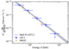 |
Fig. B.1. SED at VHE gamma rays obtained with LST-1 (blue squares) and MAGIC (orange diamonds; Acciari et al. 2022) using all observations between observation-day intervals t − t0 ∼ [1, 4] d (see Table 1 for LST-1). The best-fit model for LST-1 is displayed as a blue line together with a grey spectral error band. |
The spectral analysis of LST-1 data at observation days 1 to 4 altogether is assessed. The LST-1 joint spectral analysis follows the approach described in Sect. 2.1. The SED for the LST-1 observations right after the eruption (observation-day intervals t − t0 ∼ 1 d,2 d and 4 d, see Table 1) is shown in Fig. B.1. The best-fit model parameters for the joint analysis are tabulated in the bottom part of Table 3. The best-fit spectral model using all data right after the eruption is soft and compatible with the SED reported by Acciari et al. (2022), as shown in Fig. B.1. Nonetheless, we note that the MAGIC SED uses data from t − t0 ∼ 3 d, while LST-1 does not.
Appendix C: Robustness tests of the model fitting
Set of input reference parameter values assumed for the hadronic and leptonic model for each observation day.
To assess the stability of the fitting process for the hadronic and the leptonic models, the fitting is initialised modifying the initial parameter values of the particle energy distribution around a set of reference values (the input systematic IACT energy-scale values are set to zero for all executions). The reference initial parameters are fixed at the parameter results obtained by Acciari et al. (2022), H. E. S. S. Collaboration (2022). On the one hand, since the cutoff energy of the proton energy distribution reported by the MAGIC and H.E.S.S. Collaborations are not the same, the input cutoff energy in the fitting is established within the energy range reported by both IACT facilities. On the other hand, the assumed reference input values of the electron energy distribution are set to the best-fit results from MAGIC (see Table C.1).
A sequence of five evenly spaced values per parameter (six for the proton cutoff energy to cover the wide input parameter range) is used to define the input parameter space. The range of values we let vary for each free parameter of the particle distribution is within the 50% relative difference to the corresponding reference input parameters. The reference input parameter values in Table C.1 are included in the grid. All possible combinations of the particle energy distribution parameters are considered in the set of execution.
The vast majority of the leptonic and hadronic model fitting executions without considering systematics converge (93% and 92%, respectively). The former fitting presents more scatter of the fit results than the hadronic one likely due to the larger number of free parameters than the assumed proton spectrum shape. On the contrary, the hadronic model does not present significant variations in the output parameter values for the different input values in the parameter space. The fit results are compatible within errors for the different executions. The spread of the best-fit particle spectrum parameters at the interquartile range (IQR) for the leptonic and hadronic models without allowing for nuisance parameters describing systematics are shown in Table C.2. One can see that the slope below the energy break of the electron energy distribution (Γe, 1) presents the most significant variations. The stability of the fitting process for the leptonic model is not as robust as the fitting of the hadronic one. Therefore, the leptonic model using a BPL model cannot constrain the parameters of the electron energy distribution as precisely as the hadronic model with an ECPL.
Median and IQR statistics for the best-fit parameter distributions.
Most of the best-fit parameter values assemble forming unimodal distributions for the leptonic and hadronic models. The inclusion of LST-1 into the dataset reduces the dispersion of the distribution of the best-fit parameters. Nevertheless, two local minima are visible in the output parameter distributions for the leptonic fitting of observation day 1 (t − t0 ∼ 1 d), hence a bimodal distribution (see Fig. C.1, where the two distributions are shown in blue and black). Γe, 1 presents a local minimum peaking at negative values close to zero, while the second minimum is centred at positive values. A bump towards the positive local minimum values is also noticeable for observation day 2 (t − t0 ∼ 2 d). The two local minima are smoothly connected in the χ2 space. The local minimum close to zero peaks at a χ2 value of χ2 = 12.1, while the other minimum is centred at χ2 = 11.7. The two local minima are possible solutions for fitting the curvature of the HE spectrum. Similarly, a bimodal distribution is also obtained if we execute the fitting of the model published by Acciari et al. (2022) together with the Fermi-LAT and MAGIC data as input spectral information, yet the fitting in Acciari et al. (2022) restricted the fitting range to Γe, 1 < −0.5.
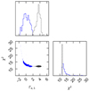 |
Fig. C.1. Corner plot of the best-fit Γe, 1 for observation day 1 and the associated χ2 fit value for different input values in the parameter space. The best-fit models used to provide the leptonic results without systematics in Table 4 are shown as solid blue lines, while the ones excluded are shown as dashed black lines (see text). |
Although the solutions with a hard electron spectrum are difficult to explain through the classical non-relativistic DSA mechanism, we extend the parameter space of the model fitting to include such solutions to study the stability of the model and provide reliable uncertainties. We report the results excluding the best-fit models with Γe, 1 > 2 (black distribution in Fig. C.1), which is the intersection value we obtain after fitting two normal distributions to the distribution of the best-fit Γe, 1 results for observation day 1 with different input parameter values (see Fig. C.1).
On the one hand, restricting the results to Γe, 1 < 2 does not significantly impact the results presented in this work for several reasons. Firstly, the best-fit slope above the energy break would not present a notable change because it is constrained by the IACT data. Whilst a slight decrease of the energy break value would result from allowing the excluded range of Γe, 1. The minor differences in these parameters would be compatible within uncertainties to the reported value in Table 4. Secondly, the physical interpretation of the excluded solutions is the same as the ones considered in the valid range (see Sect. 5). Thirdly, the improvement in the fit statistics of including such solutions is marginal. Therefore, no preference between the leptonic and hadronic models could be drawn with the AIC estimator when including these solutions. On the other hand, if the fitting range of the electron spectral slope below the energy break would had been restricted to values Γe, 1 < −0.5, as in Acciari et al. (2022), the goodness of fit of the leptonic model would have been worse than most of the output models obtained in this work (see Fig. C.1). This is attributed to the leptonic model inability to account for the positive gamma-ray emission slope below 1 GeV and posterior decay at higher energies clearly visible on observation day 1. Consequently, constraining the fitting range would have favoured the hadronic model. However, such change does not affect the fit results for observation days 2 and 4 because the emission with Fermi-LAT is dimmer and the curvature at HE gamma rays is less pronounced (p − value = 0.09 and 0.83 under the assumption of a flat HE emission for observation days 2 and 4, respectively). As a result, the best-fit leptonic model does not require a strong spectral slope break as in observation day 1 to provide a good fit. Then, both the leptonic and the hadronic models achieve comparable goodness of fit. In this manner, a nova with a brighter gamma-ray emission than RS Oph, e.g., T CrB, should help constrain the population of relativistic particles responsible for the gamma-ray emission.
The model fit results in Table 4 correspond to the best-fit execution result that is the closest one to the middle of both the AIC distribution and the particle spectrum parameter distributions obtained when varying the input value. If the energy-scale systematic distributions are considered, they are used as well. We report the uncertainties of the best-fit model parameters results as the quadratic sum of the parameter uncertainty of the fitting and the IQR of the output parameters for the different input value executions.
Despite the scattered fit results for Γe, 1, the slope above the energy break (Γe, 2) is well constrained for all days thanks to the IACT spectral information at VHE gamma rays. The use of the LST-1 spectral information is relevant to constrain the parameter space of solutions, which is narrower with the LST-1 data because of the smaller energy gap between Fermi-LAT and the IACTs data if the LST-1 SED points are considered.
Appendix D: Model fitting with systematics
When allowing for energy-scale systematics as nuisance parameters in the model fitting, the percentage of executions that converge drops to 79% and 81% for the leptonic and hadronic models, respectively, with respect to the modelling without energy-scale systematics. The output parameter distribution statistics for the modelling with systematics are shown in Table C.2. One can notice that the parameter distribution IQRs are wider when systematics are considered than when they are not. The broader distributions are expected due to the degeneracy of adding extra parameters in the model fitting to allow shifts with respect to the original SED points. Moreover, IQR values are higher for the leptonic model than the hadronic model (expected due to the worse stability of the leptonic model than the hadronic one). The local minimum peaking at positive Γe, 1 value present in the leptonic modelling without systematics vanishes when systematics are considered (see Appendix C). However, a long tail towards positive values remains.
The distributions of the best-fit IACTs energy-scale values for different input parameters form unimodal distributions. The spread of the distributions ranges all the allowed values (±15%) for most of the cases. Interestingly, the sign and the time evolution of the peak of the derived systematic energy-scale factors for MAGIC and H.E.S.S. agree with the mismatch between the spectrum from MAGIC and H.E.S.S., and the fact that the VHE gamma-ray emission increases in time, making the difference more noticeable. Figure D.1 shows the best-fit IACT systematic energy scaling factors obtained with the hadronic model for the different observation days. During observation days 1, 2 and 4, the best-daily-fit systematic energy-scale values remain below 5% for LST-1, while the sequence of MAGIC and H.E.S.S. energy scaling factors start with a low-systematic value for observation day 1 and monotonically increase in time reaching an absolute systematic energy-scale value of about 10%. MAGIC systematic values remain positive for all the observation days, while H.E.S.S. ones are negative (see Fig. D.1). As expected, no correlation between the best-fit IACT systematic uncertainties is observed.
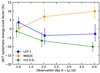 |
Fig. D.1. Derived systematic energy scaling factors for LST-1 (blue squares), MAGIC (orange diamonds) and H.E.S.S. (green circles) for the different observation-day intervals (t − t0∼ 1 d, 2 d and 4 d). The IACT systematic energy-scale value corresponds to the median value of the IACT distribution obtained with the hadronic model varying the input parameters. Error bars correspond to the IQR. |
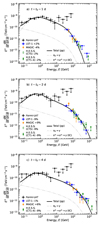 |
Fig. D.2. Same SEDs as Fig. 3 but with the IACT SED points scaled to account for the systematic energy scaling factors obtained for the best-fit hadronic model with systematics. The systematic value for each IACT is shown in the legend. In addition, the best-fit hadronic model considering energy-scale systematics is displayed as a black curve. The corresponding contributions from neutral and charged-pion decays are shown in grey. |
The addition of systematic uncertainties in the energy scale causes the differential fluxes of the IACTs to shift accordingly in the SED, both in the x- and y-axis, with respect to the original ones when the systematic energy scaling factor is different from zero. The daily SEDs adopting the best-fit systematic energy-scale factors in the IACT SED data points are shown in Fig. D.2. One can see that the differential fluxes at VHE gamma rays are concentrated in a band with less spread than the one displayed in Fig. 3 without systematic uncertainties taken into account. We note that the best-fit values of the IACT systematics in Fig. D.2 are not the same as the centre values of the IACT systematics in Fig. D.1 because the latter shows the median value and the IQR as error bars, while the former is the closest execution result with respect to both the median AIC and particle parameter distributions (see Appendix C).
Although the hadronic model with systematics effectively describes the gamma-ray emission, due to rather large statistical uncertainties on the SED data points, taking into account systematic uncertainties as extra fitting parameters (three in this case) does not impact the fit statistics enough to obtain a better fit given the reduction of degrees of freedom. Yet, systematics are foreseen to affect the SED data points. Moreover, it is worth noting that the same systematic energy-scale factor is assumed for the H.E.S.S. spectral information obtained with the array of four telescopes (CT1–4; stereo analysis) and the fifth telescope (CT5; monoscopic analysis) despite not following the exact same analysis. However, the fine agreement between both supports our simplification to reduce the number of parameters in the model fitting.
Appendix E: Lepto-hadronic model
The modelling of the RS Oph gamma-ray emission using two populations of relativistic particles, electrons and protons, is also studied. The lepto-hadronic model in Acciari et al. (2022) is considered. The particle energy distribution is assumed to follow an ECPL model, for which the cutoff energies of protons and leptons are connected by the acceleration and cooling balance (Acciari et al. 2022). Since including systematic energy-scale uncertainties as nuisance parameters are not preferred for the leptonic and hadronic models, they are excluded in the lepto-hadronic model fitting process to reduce the complexity of the fitting. The fit results are shown in Table E.1 and the best-fit model emission is shown on the daily SEDs in Fig. E.1. The same procedure as in Appendix C is followed to provide the uncertainties on the parameter values.
Model-fit results of the lepto-hadronic modelling for observation days t − t0 ∼ 1 d, 2 d and 4 d.
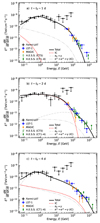 |
Fig. E.1. Same SEDs as Fig. 3 but for the best-fit lepto-hadronic model, whose total contribution is displayed as a black curve. The corresponding contributions from neutral and charged-pion decays are shown in grey and the leptonic contribution in red. |
The emission of the best-fit lepto-hadronic model on observation days 1 and 4 is dominated by proton-proton interactions in both HE and VHE bands with the spectral index and cutoff energies of the proton energy distribution consistent with the values obtained with the hadronic model (see Sect. 4.2). On the contrary, the emission at HE gamma rays on observation day 2 originates from IC losses, while the VHE component comes from proton-proton interactions. However, the best-fit model exceeds the emission constrained by the UL in the 50–100 MeV energy bin, which is important to constrain the curvature of the spectrum. For all days, the Lp/Le ratio remains high, the lowest Lp/Le ratio is  on t − t0 ∼ 2 d (see Table E.1). We note that the best-fit model is highly dependent on the input parameters. The leptonic component can contribute to the HE emission for some solutions on t − t0 ∼ 1 d, but with worse fit statistics and the VHE emission from proton-proton interactions above the SED ULs provided by the IACTs.
When comparing the AICc values of the lepto-hadronic model with the leptonic and hadronic models, the lepto-hadronic model is less preferred over them (relative likelihood of 0.014 and 0.02, respectively). Given the no preference of the lepto-hadronic model over the hadronic/leptonic model and proton-proton interactions dominate the best-fit model on t − t0 ∼ 1 d and 4 d, we disfavour this model. However, the presence of additional components in the initial gamma-ray emission cannot be excluded, but exploring this possibility would exceed the scope of this study and would require additional observations along with detailed multiwavelength modelling.
Appendix F: Akaike weights of the models
For a better interpretation of the relative likelihoods with respect to the best model according to the AIC, they are normalised to the set of positive weights that sum to 1, called Akaike weights. The information criteria measures for the different models are presented in Table F.1.
Information criteria measures for the models used in this work.
All Tables
Best-fit power-law spectral parameter values and statistical detection significances (Sig.) using LST-1 data.
Model-fit results without and with systematic uncertainties using the leptonic and hadronic modelling for observation days t − t0 ∼ 1 d, 2 d, and 4 d.
Set of input reference parameter values assumed for the hadronic and leptonic model for each observation day.
Model-fit results of the lepto-hadronic modelling for observation days t − t0 ∼ 1 d, 2 d and 4 d.
All Figures
|
Fig. 1. RS Oph daily SEDs at VHE gamma rays with LST-1 (blue squares), MAGIC (orange diamonds; Acciari et al. 2022), and H.E.S.S. (green empty squares and filled circles for the telescopes CT5 and CT1–4, respectively; H. E. S. S. Collaboration 2022) during the same day interval. From top to bottom, panels a, b, and c correspond to observation-day intervals t − t0 ∼ 1 d, 2 d, and 4 d, respectively. The best-fit model for LST-1 is displayed as a blue line together with the grey spectral error band. |
| In the text | |
|
Fig. 2. Daily integral fluxes at E > 100 GeV for LST-1 (filled blue squares) and MAGIC (filled orange diamonds; Acciari et al. 2022) as a function of MJD (bottom axis) and time after the eruption onset (top axis), which is represented as the dashed line. We also show the joint LST-1 (empty blue squares) and the joint MAGIC (empty orange diamonds) integral fluxes during observation-day intervals 1 and 4, and more than 21 days after the eruption. |
| In the text | |
|
Fig. 3. RS Oph daily SEDs from HE to VHE gamma rays using Fermi-LAT (black circles), LST-1 (blue squares), MAGIC (orange diamonds; Acciari et al. 2022), and H.E.S.S. (green empty squares and filled circles for the telescopes CT5 and CT1–4, respectively; H. E. S. S. Collaboration 2022). From top to bottom, panels a, b and c correspond to observation-day intervals t − t0 ∼ 1 d, 2 d, and 4 d, respectively. The best-fit leptonic and hadronic models are displayed as dashed red and solid black curves, respectively. For the hadronic model, the corresponding contributions from neutral and charged-pion decays are shown in grey. |
| In the text | |
|
Fig. 4. Best-fit SED models for RS Oph (black; this work, t − t0 ∼ 1 d), V906 Car (grey; Aydi et al. 2020), the first novae detected with Fermi-LAT (V407 Cyg, orange; V1324 Sco, green; V959 Mon, brown; V339 Del, pink; Ackermann et al. 2014), and the expected SED from T CrB (blue). The solid region of the nova SEDs approximately corresponds to the energy range where the model was fitted to the data, while the spaced-dashed region corresponds to the extrapolation region of the model. In addition, the sensitivity curves for LST-1 at low zenith angles (zd < 35 °; red square curves; Abe et al. 2023a) and the four LSTs of CTAO-North at zd = 20° (purple circle curves; using the latest Prod5-v0.1 IRFs in Cherenkov Telescope Array Observatory & Cherenkov Telescope Array Consortium 2021) for 5 and 50 hours of observation time (see text for details) are displayed as solid and dotted curves, respectively. |
| In the text | |
|
Fig. B.1. SED at VHE gamma rays obtained with LST-1 (blue squares) and MAGIC (orange diamonds; Acciari et al. 2022) using all observations between observation-day intervals t − t0 ∼ [1, 4] d (see Table 1 for LST-1). The best-fit model for LST-1 is displayed as a blue line together with a grey spectral error band. |
| In the text | |
|
Fig. C.1. Corner plot of the best-fit Γe, 1 for observation day 1 and the associated χ2 fit value for different input values in the parameter space. The best-fit models used to provide the leptonic results without systematics in Table 4 are shown as solid blue lines, while the ones excluded are shown as dashed black lines (see text). |
| In the text | |
|
Fig. D.1. Derived systematic energy scaling factors for LST-1 (blue squares), MAGIC (orange diamonds) and H.E.S.S. (green circles) for the different observation-day intervals (t − t0∼ 1 d, 2 d and 4 d). The IACT systematic energy-scale value corresponds to the median value of the IACT distribution obtained with the hadronic model varying the input parameters. Error bars correspond to the IQR. |
| In the text | |
|
Fig. D.2. Same SEDs as Fig. 3 but with the IACT SED points scaled to account for the systematic energy scaling factors obtained for the best-fit hadronic model with systematics. The systematic value for each IACT is shown in the legend. In addition, the best-fit hadronic model considering energy-scale systematics is displayed as a black curve. The corresponding contributions from neutral and charged-pion decays are shown in grey. |
| In the text | |
|
Fig. E.1. Same SEDs as Fig. 3 but for the best-fit lepto-hadronic model, whose total contribution is displayed as a black curve. The corresponding contributions from neutral and charged-pion decays are shown in grey and the leptonic contribution in red. |
| In the text | |
Current usage metrics show cumulative count of Article Views (full-text article views including HTML views, PDF and ePub downloads, according to the available data) and Abstracts Views on Vision4Press platform.
Data correspond to usage on the plateform after 2015. The current usage metrics is available 48-96 hours after online publication and is updated daily on week days.
Initial download of the metrics may take a while.