| Issue |
A&A
Volume 695, March 2025
|
|
|---|---|---|
| Article Number | A122 | |
| Number of page(s) | 24 | |
| Section | Stellar structure and evolution | |
| DOI | https://doi.org/10.1051/0004-6361/202451483 | |
| Published online | 12 March 2025 | |
The initial mass-remnant mass relation for core collapse supernovae
1
SISSA, via Bonomea 265, 34136 Trieste, Italy
2
Istituto Nazionale di Astrofisica - Osservatorio Astronomico di Roma, Via Frascati 33, I-00040 Monteporzio Catone, Italy
3
Kavli Institute for the Physics and Mathematics of the Universe (WPI), The University of Tokyo Institutes for Advanced Study, The university of Tokyo, Kashiwa, Chiba 277-8583, Japan
4
INFN. Sezione di Perugia, via A. Pascoli s/n, I-06125 Perugia, Italy
5
Dipartimento di Fisica, Sapienza, Università di Roma, Piazzale Aldo Moro 5, 00185 Roma, Italy
6
INFN, Sezione di Roma I, Piazzale Aldo Moro 2, 00185 Roma, Italy
7
Istituto Nazionale di Astrofisica – Istituto di Astrofisica e Planetologia Spaziali, Via Fosso del Cavaliere 100, I-00133 Roma, Italy
8
Monash Centre for Astrophysics (MoCA), School of Mathematical Sciences, Monash University, Victoria 3800, Australia
9
National Institute for Nuclear Physics – INFN, Sezione di Trieste, I-34127 Trieste, Italy
⋆ Corresponding author; This email address is being protected from spambots. You need JavaScript enabled to view it.
Received:
12
July
2024
Accepted:
30
January
2025
Abstract
Context. The first direct detection of gravitational waves in 2015 marked the beginning of a new era for the study of compact objects. Upcoming detectors, such as the Einstein Telescope, are expected to add thousands of binary coalescences to the list. However, from a theoretical perspective, our understanding of compact objects is hindered by many uncertainties, and a comprehensive study of the nature of stellar remnants from core-collapse supernovae is still lacking.
Aims. In this work, we investigate the properties of stellar remnants using a homogeneous grid of rotating and non-rotating massive stars at various metallicities.
Methods. We simulated the supernova explosion of the evolved progenitors using the HYdrodynamic Ppm Explosion with Radiation diffusION (HYPERION) code, assuming a thermal bomb model calibrated to match the main properties of SN1987A.
Results. We find that the heaviest black hole that can form depends on the initial stellar rotation, metallicity, and the assumed criterion for the onset of pulsational pair-instability supernovae. Non-rotating progenitors at [Fe/H] = −3 can form black holes up to ∼87, M⊙, thus falling within the theorized pair-instability mass gap. Conversely, enhanced wind mass loss prevents the formation of BHs more massive than ∼41.6 M⊙ from rotating progenitors. We used our results to study the black hole mass distribution from a population of 106 isolated massive stars following a Kroupa initial mass function. Finally, we provide fitting formulas to compute the mass of compact remnants as a function of stellar progenitor properties. Our up-to-date prescriptions can be easily implemented in rapid population synthesis codes.
Key words: methods: numerical / stars: black holes / stars: massive / stars: rotation / supernovae: general
© The Authors 2025
 Open Access article, published by EDP Sciences, under the terms of the Creative Commons Attribution License (https://creativecommons.org/licenses/by/4.0), which permits unrestricted use, distribution, and reproduction in any medium, provided the original work is properly cited.
This article is published in open access under the Subscribe to Open model. This email address is being protected from spambots. You need JavaScript enabled to view it. to support open access publication.
1. Introduction
On September 14, 2015, the LIGO interferometers captured a gravitational-wave (GW) signal from two merging black holes (BHs) with masses ∼36 M⊙ and ∼29 M⊙, respectively (Abbott et al. 2016a,b,c). The event, named GW150914, was the first direct detection of GWs, and provided proof that BH binaries (BHBs) exist and can merge within a Hubble time. Furthermore, prior to GW150914, there was no unambiguous evidence for stellar BHs more massive than ∼25 M⊙, which is the upper limit for the masses of BHs in known X-ray binaries (Orosz 2003; Özel et al. 2010; Miller-Jones et al. 2021). Thus, GW150914 has also provided robust evidence for the existence of heavy stellar BHs. To date, more than 90 BH-BH mergers have been reported by the LIGO-Virgo-KAGRA (LVK) collaboration (Abbott et al. 2019, 2024, 2023), and in about 70 of the events, at least one of the two BHs has a mass ≳25 M⊙. Moreover, the number of detections is expected to significantly increase in the next years because of the recent O4 LVK observing run1 and the upcoming next-generation detectors (e.g., Einstein Telescope and Cosmic Explorer).
From the theoretical point of view, the formation and the evolutionary pathways of BHs and BHBs are very uncertain (e.g., Mapelli 2021; Spera et al. 2022). Two main astrophysical formation channels have been proposed: the isolated binary evolution scenario and the dynamical formation pathway. In the former, the stellar progenitors evolve in complete isolation as a gravitationally bound pair, and they eventually turn into compact objects and merge within a Hubble time (see van den Heuvel & De Loore 1973; van den Heuvel et al. 2017; Heggie 1975; Tutukov & Yungelson 1993; Brown 1995; Bethe & Brown 1998; Sandquist et al. 1998; Dewi et al. 2006; Justham et al. 2011; Dominik et al. 2012, 2015; Schneider et al. 2015; Belczynski et al. 2016, 2018; Marassi et al. 2019a; Belczynski et al. 2020; Pavlovskii et al. 2017; Vigna-Gómez et al. 2018; Wysocki et al. 2018; Mapelli & Giacobbo 2018; Neijssel et al. 2019; Graziani et al. 2020; Mandel & Fragos 2020; Mandel & Farmer 2022; van Son et al. 2020; Broekgaarden et al. 2021; Gallegos-Garcia et al. 2021; Marchant et al. 2021; Zevin et al. 2021). In the latter, a compact-object binary forms and shrinks after a series of gravitational few-body interactions in dense stellar environments (see Sigurdsson & Hernquist 1993; Sigurdsson & Phinney 1995; Moody & Sigurdsson 2009; Banerjee et al. 2010; Banerjee 2017, 2018, 2021; Downing et al. 2011; Mapelli et al. 2013; Mapelli 2016; Ziosi et al. 2014; Rodriguez et al. 2015, 2016, 2019; Di Carlo et al. 2019, 2020b, 2021, 2020a; Rastello et al. 2019, 2020, 2021; Kremer et al. 2020; Wang 2020; Wang et al. 2022; Ye et al. 2022).
However, both the isolated and the dynamical scenarios rely on many uncertain astrophysical processes, including the core-collapse supernova (ccSN) mechanism. Our knowledge of the SN engine is still limited; thus investigating the explosion mechanism, the stellar explodability, and the mass spectrum of stellar remnants is challenging. All stars with zero-age main sequence (ZAMS) mass (MZAMS) > 9 M⊙ (Roberti et al. 2024) are expected to end their life with a ccSN and form a compact object that can be either a BH or a neutron star (NS), depending on the mass of the stellar progenitor and on the ongoing binary processes (see e.g., Doherty et al. 2017; Poelarends et al. 2017; Zapartas et al. 2017). The current reference model for ccSNe is based on the neutrino driven explosion (Bethe & Wilson 1985; Burrows et al. 1995; Janka & Mueller 1996; Janka et al. 2016; Janka 2017; Kotake et al. 2006; Herant et al. 1994; Burrows et al. 1995; Janka & Mueller 1996; Foglizzo et al. 2006; Kotake et al. 2006; Burrows et al. 2019; Aguilera-Dena et al. 2023).
State-of-the-art 3D simulations of the explosion, which include the most sophisticated treatment of neutrino transport, cannot obtain naturally and in a routine way the explosion of the star. In addition, such simulations cannot accurately constrain the amount of matter that can fall back onto the proto-compact object at later times and, consequently, the final mass of the compact remnant (see Blondin et al. 2003; Janka & Mueller 1996; Burrows et al. 1995; Suwa et al. 2010, 2013; Müller et al. 2012; Müller 2015; Summa et al. 2016; Bruenn et al. 2016; Lentz et al. 2012, 2015; Burrows et al. 2019, 2020, 2023a,b; Mezzacappa et al. 2020; Bollig et al. 2021; Wang 2020; Wang et al. 2022; Vartanyan et al. 2023; Mezzacappa et al. 2023; Powell et al. 2023; Kinugawa et al. 2021, 2024; Nakamura et al. 2025; Shibagaki et al. 2024).
A simplified approach to study the explosion of massive stars is to artificially stimulate the SN explosion by injecting some amount of kinetic energy (i.e., a kinetic bomb; see e.g., Limongi & Chieffi 2003; Chieffi & Limongi 2004) or thermal energy (i.e., a thermal bomb; see e.g., Thielemann et al. 1996) at an arbitrary mass coordinate location of the progenitor model. Alternatively, the inner edge of the exploding mantle moves outward in a manner similar to a piston following the trajectory of a projectile launched with a specific velocity in a given potential (see Woosley & Weaver 1995). Independently of the adopted techniques, the evolution of the shock is followed by means of 1D hydrodynamical simulations. The main advantage of this approach is that the computing cost is relatively small. Thus, it is possible to follow the evolution of the shock over longer timescales and to estimate the amount of fallback and the final remnant mass. The 1D approach has been extensively used to study the SN explosion yields, especially in the context of explosive nucleosynthesis (Shigeyama et al. 1988; Hashimoto et al. 1989; Thielemann et al. 1990, 1996; Nakamura et al. 2001; Nomoto et al. 2006; Umeda & Nomoto 2008; Moriya et al. 2010; Bersten et al. 2011; Chieffi & Limongi 2013; Limongi & Chieffi 2018).
Through 1D simulations, several authors have attempted to link the explodability of stellar progenitors to the structural properties of stars at the presupernova (pre-SN) stage (O’Connor & Ott 2011; Fryer et al. 2012; Horiuchi et al. 2014; Ertl et al. 2016; Sukhbold et al. 2016; Mandel & Müller 2020; Patton & Sukhbold 2020; Patton et al. 2022). Such prescriptions for the explodability have been adopted in many population synthesis codes (e.g., Eldridge et al. 2008; Spera et al. 2015; Agrawal et al. 2020; Zapartas et al. 2021; Fragos et al. 2023), to predict the final fate of massive stars and the formation and evolution of compact-object binaries in different astrophysical environments. Such analytical relations for the explodability are usually applied to stellar progenitors that are different from those employed to compute the prescriptions, and therefore must be adopted with caution. In addition, we are still far from making any conclusive statement on the final fate of massive stars. Specifically, the role played by stellar rotation, metallicity, and different stellar evolutionary models of the progenitors is still mostly unexplored.
In this work, we try to address some of these problems by studying the explosion of progenitor stars and the formation of compact remnants through the latest version of our hydrodynamic code HYdrodynamic Ppm Explosion with Radiation diffusION (HYPERION; see Limongi & Chieffi 2020), which includes a treatment of the radiation transport in the flux-limited diffusion approximation. We simulate the explosion of an up-to-date homogeneous set of both rotating and non-rotating progenitor stars provided by Limongi & Chieffi (2018, hereinafter LC18). For the SN explosion, we adopt the thermal-bomb approach, and we calibrate the parameters that describe the energy-injection process by comparison with SN1987A. We apply our methodology to investigate the distribution of remnant masses as a function of MZAMS, focusing on the role played by different initial metallicities and different values of initial stellar rotation.
In Sect. 2, we present our methodology. In Sect. 3 we present the results of our simulations. In Sect. 4 we investigate the implications of our results, and Sect. 5 contains the conclusions.
2. Methods
We used the HYPERION code to simulate the explosion of a set of pre-SN models of massive stars presented in LC18. The details of the code are discussed in Sect. 2.1.
To induce the explosion, we removed the innermost 0.8 M⊙ of the pre-SN model, and artificially deposit at this mass coordinate a given amount of thermal energy (Einj). We assumed that Einj is diluted both in space, over a mass interval dminj, and in time, over a time interval dtinj. Therefore, our numerical approach relies on the three free parameters Einj, dminj, and dtinj, which need to be calibrated. The details of the calibration are presented in Sect. 2.2.
Once the energy is deposited into the pre-SN model, a shock wave forms. The shock wave starts to propagate outwards and eventually drives the explosion of the star. While the shock advances, it induces explosive nucleosynthesis and accelerates the shocked matter. After the initial energy injection, the innermost regions begin to fall back onto the proto-compact object, which progressively increases its mass. After the end of the fallback phase, we define the “mass cut” as the mass coordinate that divides the final remnant from the ejecta. Depending on the position of the mass cut, we can recognize two possible outcomes of our simulations: successful explosion, if a substantial fraction of the envelope is ejected during the explosion (the simulated physical time is of 1 yr, ∼3 × 10⁷ s, which is sufficient to follow also the homologous expansion of the ejected matter in the circumstellar medium and the formation of the light-curve), or failed explosion if essentially the whole star collapses to a BH. The former case is presented in Sect. 3.1, while the latter is discussed in Sect. 3.2.
2.1. The HYPERION code
In this section, we briefly describe HYPERION, which is the 1D hydrodynamical code we adopt in this work and which was presented in detail in Limongi & Chieffi (2020). The code solves the full system of hydrodynamic equations (written in a conservative form) supplemented by the equation of the radiation transport (in the flux-limited diffusion approximation) and the equations describing the temporal variation of the chemical composition due to the nuclear reactions. Such system of equations can be divided into two parts. The first part includes the hydrodynamical equations and the radiation transport:
 (1)
(1)
 (2)
(2)
 (3)
(3)
where ρ is the density, r is the radial coordinate, v is the velocity, m is the mass coordinate, P is the pressure, E is the total energy per unit of mass, L is the radiative luminosity, and ϵ is any source and/or sink of energy (e.g., nuclear reactions, neutrino losses).
The second part describes the variation of chemical composition caused by nuclear reactions:
 (4)
(4)
where N is the number of nuclear species included in the calculations, Yi is the abundance by number of the i-th nuclear species, Λ refers to the weak interactions or the photodissociation rate, depending on which process is in place for the j nuclear species, and  represents the two or three-body nuclear cross section (see Limongi & Chieffi 2018 and Limongi & Chieffi 2020 for a detailed discussion).
The terms on the right side of Eq. (4) describe the contribution to the abundance due to various physical processes, such as: (1) the β-decay, electron-captures, and photodisintegrations; (2) two-body reactions; (3) three-body reactions. The coefficients in Eq. (4) are defined as
 (5)
(5)
 (6)
(6)
 (7)
(7)
where Ni refers to the number of i particles involved in the reaction, and the factorial terms prevent from double counting the reactions with identical particles. The sign (+)/(-) depends on whether the i particles are created or destroyed. Finally, the radiative luminosity in the flux-limited diffusion approximation is defined as
 (8)
(8)
where a is the radiation constant, c is the speed of light, κ is the Rosseland mean opacity, and λ is the flux limiter, computed according to Levermore & Pomraning (1981) as:
 (9)
(9)
with
 (10)
(10)
The Rosseland mean opacities are calculated for a scaled solar distribution of all elements, corresponding to Z = Z⊙ = 1.345 × 10⁻² ([Fe/H] = 0) (Asplund et al. 2009). At lower metallicities, we consider an enhancement of C, O, Mg, Si, S, Ar, Ca, and Ti with respect to Fe, accordingly to observations (Cayrel et al. 2004; Spite et al. 2005). As a result of the enhancement, we find that metallicity indexes [Fe/H] = −1, −2 and −3, correspond to metallicity values of Z = 3.236 × 10⁻³ (2.406 × 10⁻¹ Z⊙), Z = 3.236 × 10⁻⁴ (2.406 × 10⁻² Z⊙), and Z = 3.236 × 10⁻⁵ (2.406 × 10⁻³ Z⊙ ), respectively.
We adopt opacity tables from three different sources, depending on the temperature regime. In the low-temperature regime (2.75 ≤ log T/K ≤ 4.5), we refer to Ferguson et al. (2005), in the intermediate-temperature regime (4.5 ≤ log T/K ≤ 8.7) to Iglesias & Rogers (1996), and for higher temperatures we adopt the Los Alamos Opacity Library (Huebner et al. 1977).
Lastly, the equation of state (EOS) is the one described in Morozova et al. (2015), based on the analytic EOS of Paczynski (1983), which takes into account radiation, ions, and electrons in an arbitrary degree of degeneracy. The H and He ionization fractions are obtained by solving the Saha equations, as in Zaghloul et al. (2000), while we assume that all other elements are fully ionized.
The energy generated through nuclear reactions is neglected, because we assume that its contribution is negligible compared to other energy sources, but we consider the energy deposition from γ-rays that comes from the radioactive decays  and
and  , following the scheme described in Swartz et al. (1995) and Morozova et al. (2015).
To solve the hydrodynamic equations, we use a fully Lagrangian scheme of piece-wise parabolic method (PPM) presented in Colella & Woodward (1984). To implement that, we first interpolate the profiles of the variables ρ, v, and P as a function of the mass coordinate, using the interpolation algorithm of Colella & Woodward (1984). Then, we solve the Riemann problems at every cell interfaces. Thus, we obtain the time-averaged values of pressure and velocity at the zone edges. Finally, we update the conserved quantities by applying the forces resulting from the time-averaged pressures and velocities at the zone edges, following the scheme presented in Limongi & Chieffi (2020).
2.2. Calibration of the explosion
During the explosion, the innermost zones of the stellar mantle are heated up by the expanding shock wave to temperatures high enough to induce explosive nucleosynthesis. One of the main products of the nucleosynthesis is 56Ni, which is synthesized by the explosive Si burning in the innermost regions of the mantle (Thielemann et al. 1996; Woosley & Weaver 1995; Arnett & Chevalier 1996; Limongi et al. 2000). Therefore, the location of the mass cut is crucial to constrain the amount of ejected 56Ni: in absence of mixing, the more external the mass cut, the lower the abundance of nickel in the ejecta. Another important outcome of our simulations is the final kinetic energy of the ejecta, which comes from the conversion of a fraction of the thermal energy initially injected into the progenitor star. The amount of ejected 56Ni and the final kinetic energy of the ejecta depend on the explosion parameters, i.e. Einj, dminj, and dtinj. We calibrated these parameters considering SN1987A, which is the most extensively studied ccSN to-date (e.g., Arnett et al. 1989; Woosley 1988). Specifically, our goal was to find the combination of the explosion parameters that match both the ejected 56Ni and the kinetic energy of the ejecta with the values estimated for the SN 1987A, that is, m and ∼1051 erg = 1 foe (see, e.g., Arnett et al. 1989; Shigeyama & Nomoto 1990; Utrobin 1993, 2006; Blinnikov et al. 2000). To reach our goal, we simulated the explosions of the stellar progenitor of our grid that best match the helium core of the progenitor of SN 1987A (i.e., Sk – 69°202 e.g., Woosley 1988; Arnett et al. 1989; Arnett & Chevalier 1996, with MHe ∼ 6 M⊙, e.g., Woosley 1988). We made this choice because Eejecta and m56Ni do not depend on the structure of the hydrogen envelope of the star.
Therefore, we adopted a 15 M⊙-progenitor model with initial solar composition ([Fe/H] = 0, i.e. the model 15a000 in the set of LC18) and, in each simulation, we adopted a different set of explosion parameters. Figure 1 shows the final kinetic energy of the ejecta and the corresponding amount of ejected 56Ni obtained from our simulations using different explosion parameters, with Einj ∈ [1.9 ; 2.1] foe, dminj ∈ [0.05;0.4] M⊙, and dtinj ∈ [10−9 ; 1] s.
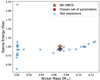 |
Fig. 1. Final kinetic energy of the ejecta as a function of the ejected mass of 56Ni obtained running various explosion tests (blue crosses) with different values of the initial explosion parameters, Einj, dminj, and dtinj. The red dot refers to the simulation of the explosion that best matches the properties of SN1987A (orange star). |
The combination of explosion parameters that best matches the values of SN1987A is: dtinj = 0.01 s, dminj = 0.1 M⊙, and Einj = 2.0 foe. We adopted this combination of explosion parameters in all the simulations presented in this work. Using the calibrated values of Einj, dminj, and dtinj, we computed the explosion of a subset of the pre-SN models presented in LC18.
Finally, it is important to mention a significant caveat that may influence these results. Podsiadlowski (1992) and Menon & Heger (2017) suggest that Sk – 69°202, the progenitor of SN1987A, might have originated from a stellar merger. This scenario introduces uncertainties in the final He core mass of the progenitor and, consequently, in the dynamics of the explosion. However, SN1987A is widely used in the literature (e.g., Ugliano et al. 2012; Ertl et al. 2016; Sukhbold et al. 2016, 2018) as a benchmark to tune the parameter describing the supernova explosion mechanism. Adopting this approach remains essential for facilitating comparisons with other studies.
2.3. Progenitors unstable against pair production
Figure 2 shows the mass at the pre-SN stage MpreSN and the carbon-oxygen (CO) core mass MCO of the stars of our simulations grid as a function of MZAMS. The properties of the models for which we perform the explosions are also summarized in Table C.2 and Table C.3.
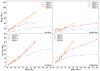 |
Fig. 2. Mass at the pre-SN stage (top-row panels) and CO core mass (bottom-row panels) as a function of MZAMS for the non-rotating progenitors (left panels) and progenitors rotating with an initial velocity of 300 km/s (right panels). Different colors represent different initial metallicities: [Fe/H] = 0 (dashed light blue line), [Fe/H] = −1 (dash-dotted violet line), [Fe/H] = −2 (orange solid line), and [Fe/H] = −3 (dotted yellow line). |
In our grid of non-rotating stellar models, we find that at subsolar metallicities the non-rotating stellar progenitors with MZAMS = 80 M⊙ end their life as ccSNe with CO core masses of ∼30 M⊙, while the 120 M⊙-progenitors become unstable (i.e., the adiabatic index Γ1 approaches the critical value of 4/3 in a substantial fraction of the core) and start entering the pair-instability phase (Fowler & Hoyle 1964; Barkat et al. 1967; Rakavy & Shaviv 1967). Thus, the progenitors unstable against pair production start to evolve on the hydrodynamical timescale and the Frascati Raphson Newton Evolutionary Code (FRANEC) code cannot follow the evolution of the stellar structure anymore. Furthermore, pulsational pair-instability supernovae (PPISNe) are very different from the ccSNe HYPERION is designed to deal with, thereby we cannot simulate the final stages of massive stars that develop pair instabilities.
Finally, the mass resolution of the pre-SN simulated grid does not allow us to determine the mass threshold for the onset of the PPISNe; from our data, the only thing we know is that 120 M⊙ progenitors at sub-solar metallicity are unstable against pair production, while the 80 M⊙ progenitors are not. In order to determine which is the minimum mass of the CO core that enters the PPISNe regime ( ) and the minimum one that enters the pair-instability supernova (PISN) regime (
 ), we can refer to the values provided by Heger & Woosley (2002) (hereinafter HW02) and Woosley (2017) (hereinafter W17), i.e.
  and
and  , respectively. These two values are in a good agreement with the LC18 models (
 ), within the theoretical uncertainties. Additionally, it should be noted that, in W17, the pulses associated with a CO core mass of MCO = 28 − 31 M⊙ are quite weak, and the first significant pulse occurs at a CO core mass of approximately 33 M⊙. Hence, we adopt
  as the minimum CO core mass that enters the PPISN. Furthermore, since the liming masses obtained in both cases (i.e., HW02 and W17) are compatible with the results of LC18. In the following, we refer to and use the results provided by W17. Finally, following W17, stars with CO core mass ≥54 M⊙ are completely disrupted by PISNe. This value corresponds to an initial mass which is larger than the maximum mass considered in our SN grid.
Independently of the rotation rate and metallicity, Figure 2 shows that MpreSN and MCO scale linearly with MZAMS. Therefore, to find the values of MZAMS and MpreSN of the first progenitor unstable against pair instabilities we assumed:
 (11)
(11)
 (12)
(12)
where k1 and q1 (k2 and q2) are the slope and intercept of the line MCO ‘vs’ MZAMS (MpreSN ‘vs’ MZAMS).
Therefore, according to both W17, we find  for the various metallicities and rotation velocities that are reported in Table C.1. Specifically, in Table C.1 we report, for all the initial values of metallicity and angular rotation, the values of
  and
and  that we obtained for the last progenitors stable against pair-instabilities. When the heaviest stars of our pre-SN grid are stable against pair-production, we cannot predict for which values of MZAMS they will become unstable against pair-instability (i.e., which stellar progenitors will explode as PPISNe or PISNe). Thus,
  and
and  are labeled as “Not Available” (N.A.) in Table C.1.
3. Results
In this section, we present the results of the simulations performed in the pre-SN models described in Figure 2 and Tables 2 and 3 (see also LC18). We simulated the explosions for all the models with pre-SN CO core masses ≤33 M⊙ because these models are considered stable against pair production, as in LC18 (see Sect. 2.3). The results of the simulations are also summarized in Tables C.2 and C.3.
3.1. Successful explosions
To illustrate the properties of a typical successful explosion in our simulations, we consider a non-rotating 25 M⊙ star with metallicity [Fe/H] = −2. Figure 3 shows the chemical structure of the model which is characterized by an extended H-rich envelope, with a He core mass of 9.87 M⊙ and a CO core mass of 5.95 M⊙. The oxygen-neon (ONe) shell extends from mass coordinate 1.73 M⊙ to 5.17 M⊙, while the Si shell, which is enriched by the products of the O-shell burning, is in the range 1.43 M⊙–1.73 M⊙. The mass of the iron core is therefore 1.43 M⊙.
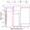 |
Fig. 3. Chemical composition as a function of the interior mass coordinate of a non-rotating model with MZAMS = 25 M⊙ and [Fe/H] = −2 at the pre-SN stage. We show the chemical composition up to the mass coordinate of 15 M⊙. We report the abundances of H (black line), He (red line), 12C (green line), 16O (blue line), 20Ne (magenta line), 28Si (orange line), 52Cr (dark red line) and 56Fe (gray line). |
Figure 4 shows the temperature and density profiles of the star at the pre-SN stage. During the pre-SN evolution, the progenitor loses a negligible amount of mass because of its initial low metallicity and has a low effective temperature of ∼ 4.7 × 10³ K. Thus, it ends its life as a Red Super Giant (RSG, Limongi & Chieffi 2018).
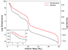 |
Fig. 4. Temperature profile (solid red line) and mass density profile (dash-dotted black line) of the stellar progenitor at the pre-SN stage as a function of the mass coordinate. A zoom-in on the innermost region of the core, up to 5 M⊙, is highlighted in the lower-left box. |
The density profile (see Figure 4) shows gradients at mass coordinates which correspond to boundaries between shells of different chemical composition. The most prominent density gradient is at the mass coordinate of ∼10 M⊙ and it corresponds to the interface between the He core and the H envelope. The injection of thermal energy into the iron core results in the formation of a shock wave that moves outward in mass and compresses, heats up, and accelerates the overlying layers. Once the shock emerges from the iron core, it propagates through the outer layers, where it triggers the explosive nucleosynthesis. Figure 5 shows the evolution of the velocity profile of the shock wave at different times after the onset of the explosion. After ∼ 0.7 s, the shock wave reaches the mass coordinate of ∼2.7 M⊙, where the peak temperature of the shock becomes too low to trigger any other additional burning. Therefore, from this mass coordinate outward, the chemical structure sculpted by the hydrostatic evolution will be unaffected by the passage of the shock wave.
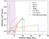 |
Fig. 5. Velocity of the shock wave as a function of the mass coordinate at different times after the onset of the explosion. The end of the explosive nucleosynthesis (dotted blue line), the shock wave enters the CO core (dash-dotted orange line), the shock wave reaches the He/H interface (solid green line), 1000 s after the onset of the explosion (dashed red line), the formation of the compact remnant (long dashed purple line), and the shock breakout (short dot-dashed light green line). The shaded purple area represents the extension of the final compact remnant. |
After 15.5 s from the beginning of the explosion, while the shock is still moving through the CO core, some of the innermost layers (i.e. the inner ∼2 M⊙) revert their motion because their velocity is lower than the local escape speed (see the negative values of the orange line in Figure 5).
At ∼ 100 s, the shock reaches the He/H interface at a mass coordinate of ∼10 M⊙, where a strong density gradient (see Figure 4) causes the formation of a reverse shock (see Woosley & Weaver 1995). From this time onward, the explosion is characterized by a shock wave moving outward in mass and by a reverse shock, which propagates inward in mass, slowing down the previously accelerated material. This effect is apparent from the behavior of the velocity of the shock 1000 s after the onset of the explosion (red dashed line in Figure 5), for which we find that the velocity of the outer regions of the shock is smaller than that of the innermost regions of the shock wave. This happens because the latter have not yet been affected by the reverse shock at this stage of the explosion.
Furthermore, Figure 5 shows also that when the shock reaches the He/H interface, the compact remnant increases its mass up to ∼2 M⊙, since the layers which had negative velocity when the shock has reached the CO core have now reached zero velocity.
The fallback process eventually ends ∼ 3 × 10⁴ s after the onset of the explosion, leaving a compact remnant with a final mass of 5.77 M⊙ (the purple shaded area in Figure 5). It is worth noting that such a heavy compact remnant includes also the layers where the explosive nucleosynthesis happened (≲2.7 M⊙, i.e. the Si and ONe shells, see Figure 3), preventing their ejection into the interstellar medium unless some mixing of material from the innermost zones to the outer layers is occurring during the explosion. Finally, ∼ 1.5 × 10⁵ s (i.e. ∼1.7 days) after the beginning of the explosion, the forward shock reaches the surface of the star (shock breakout).
Figure 6 shows the kinetic energy, the sum of internal and gravitational energy, and the total energy of the star as a function of the mass coordinate, at times > 15 seconds after the onset of the explosion. From this figure it is apparent that, at each time, some regions are falling back onto the proto-compact object (i.e. those with negative total energy) and some are being expelled by the shock wave (i.e. those with positive total energy). The last region with negative total energy corresponds to the boundary of the final remnant, that is represented in Figure 6 with a purple shaded area.
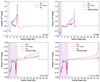 |
Fig. 6. Interior profiles of the kinetic energy (yellow line), the internal energy plus the gravitational energy (purple line), and the total energy (dashed light blue line) at various times during the explosion for a non-rotating stellar progenitor with MZAMS = 25 M⊙ with metallicity [Fe/H] = −2. The shaded purple area in the panels represents the region of the star forming the compact remnant at each time. It is completely formed at t = 3 × 10⁴ s. |
We present the whole process in Figure 7, which shows the evolution of the radius of various mass shells (gray, in step of 1 M⊙, and dotted red lines, in step of 3 M⊙) inside the stellar progenitor as a function of time. From this figure we can distinguish the layers of the star that fall back onto the compact object, i.e., those that form the final remnant (represented by the dashed yellow line), and those that are successfully ejected at the shock breakout. Roughly at ∼10 s we find that the radius of the mass shells corresponding to the most internal 2 M⊙ of the star (the first two gray lines) revert their trajectory, start to fall back onto the proto-compact object, and they reach the latter ∼100 s after the onset of the explosion.
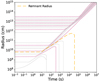 |
Fig. 7. Evolution of the radius of various shells (gray and dotted purple lines) inside the stellar progenitor as a function of time. Each gray (dotted purple) line on top encloses 1 M⊙ (3 M⊙) more than the gray (dotted purple) line immediately below. We also show the evolution of the radius of the final compact remnant (yellow dashed line). |
Figure 7 also shows when the fallback ends. The last shell that falls back onto the compact object reverts its trajectory roughly ∼104 s after the onset of the explosion and it reaches the compact remnant at t = 3 × 10⁴ s (consistent with our results reported in Figure 5 and in the bottom left panel of Figure 6). For t ≥ 3 × 10⁴ s, such mass shell has zero velocity forming the final remnant with mass 5.77 M⊙. In Figure 7 all the layers that eventually form the final remnant are shown to instantaneously drop onto the compact remnant, but this is only a numerical effect, since once they revert their trajectory, falling back onto the BH, we no longer followed their evolution. That is, we did not observe the free fall trajectories. In contrast, the outer region is eventually ejected by the shock wave at the shock breakout, and it keeps moving outward in the interstellar medium with a radial velocity that grows linearly with time.
3.2. Direct collapse
The progenitor model we adopt to describe a typical failed explosion which undergoes a direct collapse (DC) to BH in our simulations is a non-rotating 80 M⊙-star with metallicity [Fe/H] = −2. Figure 8 shows the chemical structure of the star at the pre-SN stage. The structure is characterized by an extended H-rich envelope, a He core mass of 38.3 M⊙ and a CO core mass of 28.9 M⊙. The ONe shell extends between mass coordinate 4.33 M⊙ and 14.9 M⊙ while the Si shell extends from 1.76 M⊙ to 4.33 M⊙. The mass of the iron core is 1.76 M⊙.
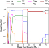 |
Fig. 8. Chemical composition as a function of the interior mass coordinate of a non-rotating model with MZAMS = 80 M⊙ and [Fe/H] = −2 at the pre-SN stage. We report the abundances of H (long dash-double dotted black line), He (double dash-dotted red line), 12C (long dashed green line), 16O (short dashed blue line), 20Ne (dashed magenta line), 28Si (short dash-double dotted orange line), 52Cr (solid dark red line) and 56Fe (long dash-dotted gray line). |
Figure 9 shows the temperature and the density profile of the progenitor as function of the mass coordinate. From this figure it is apparent that the density profile presents various steep density gradients, each one corresponding to the boundaries between shells of different chemical composition. As in the previous case of a successful explosion, this star loses a negligible amount of mass during its life because of its initial low metallicity and it reaches the pre-SN phase as a RSG, having an effective temperature of 6.3 × 10³ K.
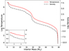 |
Fig. 9. Temperature profile (red line) and density profile (dash-dotted black line) at the pre-SN stage as a function of the mass coordinate of a non-rotating stellar progenitor with MZAMS = 80 M⊙ and [Fe/H] = −2. A zoom-in on the innermost region of the core, up to 5 M⊙, is highlighted in the lower right box. |
In Figure 10, we show the velocity profile of the explosion as a function of the mass coordinate at different times after the onset of the explosion. Figure 10 shows that the velocity of the shock progressively decreases with time. The regions behind the shock wave begin reverting their trajectory ∼1.5 s after the onset of the explosion, since they have exhausted their initial kinetic energy. Thus, they start falling back onto the proto-compact object with negative radial velocity. As the shock moves at larger mass coordinates, more and more internal layers exhaust their kinetic energy, and fall back onto the core, until the velocity of the shock becomes almost zero at ∼ 36 s after the onset of the explosion. Therefore, in this case, the shock wave does not have enough energy to eject the mantle of the star.
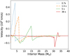 |
Fig. 10. Same as Figure 5 but for a directly collapsing progenitor. The velocity profile is reported at different crucial times during the explosion: when the explosive nucleosynthesis stops (dotted blue line), when the layers behind the shock start to fallback onto the compact remnant (dash-dotted orange line), when the shock enters the CO core (dashed green line) and when the velocity of the shock becomes negligible (solid red line). |
Figure 11 shows the dynamics of the innermost layers of the stellar progenitor. Such layers undergo a brief acceleration phase when the shock wave reaches them. However, such acceleration is not sufficient to unbound these regions from the star. In Figure 11 we notice the same behavior we presented in Figure 10: already ∼1.5 s after the onset of the explosion, the innermost layers of the star revert their trajectory, falling back onto the proto-compact object, reaching the latter only a few seconds later, and becoming part of the final remnant at ∼5 s. Furthermore, the acceleration decreases in the outer layers, which start to collapse again immediately after the passage of the shock wave. Therefore, the latter cannot reach the surface of the star and the entire progenitor directly collapses into a heavy BH.
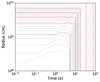 |
Fig. 11. Same as Figure 7 but for the most central region of the progenitor with MZAMS = 80 M⊙ and [Fe/H] = −2, where we can better appreciate the fallback of the layers right after being accelerated by the shock wave. We show the behavior of the shell enclosing different values of mass, of 1 M⊙ (each solid light gray lines) and 5 M⊙ (each dotted purple line), respectively. |
3.3. Remnants black holes from non-rotating progenitors
Figure 12 shows the remnant masses as a function of MZAMS, for non-rotating progenitors and for various initial metallicities. From Figure 12 it is apparent that the remnant mass increases as a function of MZAMS for all the considered metallicities. Furthermore, the remnant mass is larger for progenitors at lower metallicities, and does not depend significantly on metallicity for progenitors with MZAMS ≲ 25 M⊙.
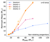 |
Fig. 12. Remnant masses as a function of MZAMS for the progenitors with initial metallicity [Fe/H] = 0 (dashed light blue line), [Fe/H] = −1 (dash-dotted violet line), [Fe/H] = −2 (orange solid line), and [Fe/H] = −3 (dotted yellow line). We do not simulate the explosion of the stellar progenitors with MZAMS = 120 M⊙ at subsolar metallicities, since they are unstable against pair production. |
The remnant mass curves follow closely the behavior of the CO core mass (see the bottom-left panel of Figure 2).
This happens because the remnant mass depends on the binding energy of the star at the pre-SN stage, and that comes mainly from the CO core. Moreover, larger CO core masses imply lower  mass fractions at core-He depletion, i.e. a less efficient C-shell burning, which, in turn, causes a higher contraction of the CO core resulting in a more bound structure.
Figure 13 shows the mass of the progenitor star at the pre-SN stage and the mass of the compact remnant as a function of the initial mass of the star, for various metallicities. In our simulations, we assume that DC occurs if the fraction of the progenitor’s envelope ejected by the shock wave is less than 10% of the pre-SN mass. For example, the progenitor at solar metallicity with MZAMS = 60 M⊙ has a pre-SN mass of 16.9 M⊙ and forms a remnant of 16.2 M⊙, ejecting only 0.7 M⊙ of H envelope; thus we consider it a DC. Following this approach, we find that stars with MZAMS ≳ 60 M⊙ do not explode and collapse directly to a BH for the initial metallicities [Fe/H] = 0, [Fe/H] = −2, [Fe/H] = −3. For [Fe/H] = −1, the threshold for DC is MZAMS = 80 M⊙. This happens because the progenitor with MZAMS = 60 M⊙ ends its life as a RSG. Thus, the shock wave ejects part of the H envelope since this is very loosely bound to the star (see Fernández et al. (2018)). This happens only for this value of metallicity, because at [Fe/H] = 0 the star with MZAMS = 60 M⊙ has already lost all its H envelope at the pre-SN stage, while at [Fe/H] = −2 and [Fe/H] = −3 stellar winds are quenched, i.e. all the H envelope is retained and the star is much more compact.
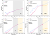 |
Fig. 13. Pre-SN mass (dash-dotted light blue line), pre-SN mass extrapolated for MZAMS > 120M⊙ (dotted gray line), remnant mass (solid violet line), and the remnant mass for the stars that develop pair instabilities (dashed yellow line), as a function of MZAMS. The red points represent the stellar progenitors of the FRANEC grid, while the larger red squares correspond to the last progenitor stable against pair production, which has been obtained through interpolation (see Sect. 2.3 and Table C.1). The shaded gray area represents the region of DC, the shaded yellow area shows where stars undergo PPISNe. The vertical dashed lines represent the threshold values above which stars enter the PI regions. |
We do not account for additional mass loss effects associated with DC (e.g., from neutrino emissions, as proposed by Nadezhin 1980; Piro 2013). In our simulations, all massive stars that end their lives through DC are compact BSG stars. Therefore, such effects are negligible (see Lovegrove & Woosley 2013; Fernández et al. 2018), as they primarily affect more extended stars like RSGs. However, in our simulations such stars naturally lose their H envelope as a consequence of the shockwave.
The BH masses at the threshold for DC depend on the final mass of the progenitor stars at the pre-SN stage that, in turn, depends on the mass-loss history during the pre-SN evolution. The mass-loss rate decreases significantly at low metallicity, where stellar winds are quenched. Therefore, the models with initial metallicity lower than [Fe/H] = −1 evolve approximately at constant mass. As a consequence, the BH masses correspond to the threshold in MZAMS for DC (see Table C.1). Above  we compute the remnant masses taking into account the results of W17 (see, e.g., its Table 1) by interpolating on the CO core mass.
The results are shown in Figure 13 as yellow diamond points and are connected through the dashed yellow lines. From this figure it is apparent that at [Fe/H] = −1 the onset of PPISNe does not affect significantly the maximum BH mass that forms. This happens because – at the pre-SN stage – stars have already lost a significant part of their H envelope. Thus, the mass loss caused by PPISNe does not affect significantly the final BH mass. In contrast, for [Fe/H] = −2, −3, stars evolve at almost constant mass and end their life with heavy H envelopes. Therefore, the expulsion of the latter at the onset of PPISN significantly affects the final BH mass. This effect is apparent in the bottom-row panels of Figure 13, where we see a steep variation of the final remnant mass at the onset of PPISNe.
3.4. Remnants black holes from rotating progenitors
Figure 14 shows the remnant masses as a function of MZAMS, for rotating progenitors and for various initial metallicities. From Figure 14 it is apparent that, at solar metallicity, the remnant mass does not increase significantly with the initial progenitor mass. In contrast, for [Fe/H] = −1, −2, −3, the remnant mass curve has a local minimum at 25 M⊙, which occurs when the stellar winds are strong enough to completely remove the H envelope. Furthermore, as in the case of the non-rotating progenitors, for MZAMS ≳ 25 M⊙ the remnant masses are larger at lower metallicities, and follow the behavior of the CO core mass at the pre-SN stage (see also Sect. 3.3).
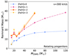 |
Fig. 14. Same of Figure 12 but for rotating progenitors. We do not simulate the explosion of the stellar progenitors with MZAMS = 80 M⊙ and 120 M⊙ at [Fe/H] = −2, −3, since they are unstable against pair production. |
Figure 15 shows how the remnant mass and the mass of the star in the pre-SN phase depend on MZAMS, for rotating models with different initial metallicities. We find that most of the rotating progenitors directly collapse to BHs. This happens because rotating stars end their life as He-stars, that is, they end their life with more bound structures at the pre-SN stage with respect to non-rotating progenitors, and thus they are more prone to failed SN explosions and to form more massive BHs. Specifically, stars with MZAMS ≳ 30 M⊙ collapse directly to a BH, whereas the fate of stars with MZAMS ≲ 30 M⊙ depends on the initial metallicity.
At solar metallicity, the threshold value of MZAMS for the DC decreases down to ∼20 M⊙, since only the progenitor with MZAMS = 15 M⊙ evolves through a successful SN explosion. At [Fe/H] = −1, the only exploding progenitor is the one with MZAMS = 25 M⊙, and it ejects all its H envelope, while the less massive progenitors directly collapse to BHs. Although this occurs only for one progenitor in the simulation set, the non-monotonic behavior for the explodability is not apparent for non-rotating progenitors (see Figure 13). At [Fe/H] = −2, all the progenitors evolve through DC. The progenitor with MZAMS = 20 M⊙ ejects some material but it is still consistent with our definition of DC, and thus the threshold value of MZAMS for the DC is ∼15 M⊙. The stars at [Fe/H] = −3 behave similarly to solar metallicity models, and the only exploding progenitor is the one with MZAMS = 15 M⊙; thus the threshold of MZAMS for the DC is at ∼20 M⊙.
For rotating progenitors, mass loss is enhanced because rotation forces the models to become red giants and therefore to approach their Eddington luminosity during their redward excursion in the HR diagram (see LC18). When this happens, a substantial amount of mass is lost and most of the stellar models loose all their H rich envelope and become Wolf-Rayet stars. Therefore, progenitors with the same MZAMS and metallicity retain less mass at the pre-SN stage than non-rotating stars. This is apparent especially at lower metallicities, where stellar winds for non-rotating progenitors are quenched. This effect is not significant for progenitors with MZAMS ≤ 30 M⊙, since such stars have weak stellar winds. As a consequence, we obtain less massive BHs from rotating stellar progenitors than from non-rotating ones.
The BH masses corresponding to the threshold in MZAMS for the DC are ∼8 M⊙, ∼16 M⊙, ∼14 M⊙ and ∼20 M⊙ for metallicities [Fe/H] = 0, [Fe/H] = −1, [Fe/H] = −2, [Fe/H] = −3, respectively. The threshold CO core mass for PPISNe,  are reported in Table C.1.
To estimate the remnant masses of the models with  we apply the results of W17, as described in Sect. 3.3. The results of such interpolations are the diamond yellow points, which are connected through the dashed yellow lines. From Figure 15, it is apparent that, for rotating stellar progenitors, there is no major change in the BH mass due to the onset of PPISNe. This happens because the rotating stars end their life as naked He stars; thus they have lost their H envelope. Therefore, the rotating stars only lose a small fraction of their He core at the onset of the PPISNe, because of the pulsational phase, and then collapse to BHs.
4. Discussion
4.1. The maximum black hole mass
Figure 16 shows the maximum BH mass resulting from our simulations as a function of the initial stellar metallicity, and assuming rotating and non-rotating single star models. It illustrates the impact of the initial metallicity and angular rotation of the stellar progenitor on the final remnant mass we obtain from single stellar evolution.
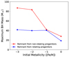 |
Fig. 16. Maximum BH mass as a function of the initial metallicity for the non-rotating stellar progenitors (red line) and the rotating stellar progenitors (blue line) for the non-rotating progenitors. |
For [Fe/H] = 0 and [Fe/H] = −1, stellar winds play a crucial role as they remove a significant fraction of mass of the progenitor stars before they DC to BHs. From our simulations, we find that the maximum BH mass we form is ∼27.9 M⊙ and ∼41.9 M⊙, for [Fe/H] = 0 and [Fe/H] = −1 in the non-rotating case, and ∼18.6 M⊙ and ∼40.5 M⊙, for [Fe/H] = 0 and [Fe/H] = −1 in the rotating case. All these BHs come from the collapse of stellar progenitors with MZAMS = 120 M⊙. Therefore, we find that angular rotation slightly enhances the effects of the stellar winds at solar metallicity, while at [Fe/H] = −1 the effect of rotation on the final remnant masses is negligible. For the cases [Fe/H] = −2, −3 the heaviest BHs from non-rotating stellar progenitors have mass ∼83.3 M⊙ and ∼87.0 M⊙ respectively, and they both correspond to stellar progenitors with MZAMS ≃ 87 M⊙ (as reported in Table C.1). In the rotating case, the maximum BH mass is ∼39.9 M⊙ and ∼41.6 M⊙ for [Fe/H] = −2 and [Fe/H] = −3, respectively, and they correspond to stellar progenitors with MZAMS ≃ 65 M⊙ (see Table C.1). Therefore, in the rotating scenario, the initial angular rotation enhances mass loss and induces the formation of larger convective regions and therefore larger CO cores (see LC18, Marassi et al. 2019b, and Mapelli et al. 2020). As a consequence, stars are less massive at the pre-SN stage and enter the PPISNe regime at lower initial masses compared to non-rotating progenitors. Such a combination of effects limits significantly the value of the maximum BH mass.
4.2. Implications for the PI mass gap
Figure 16 shows that we can form heavy BHs that lie in the upper mass gap predicted by PISN models, i.e. a dearth of BHs with masses in the range 60 − 120M⊙ (e.g., Woosley 2017; Spera & Mapelli 2017). This is because we can form BHs in the upper mass gap because the FRANEC progenitors enter the pair-instability at different initial progenitor masses than those of other authors (e.g., Woosley 2017; Spera & Mapelli 2017; Farmer et al. 2019; Costa et al. 2021).
Given our choice of the minimum CO core pass for the onset of PPISN of 33 M⊙ (see Sect. 2.3), we find that, for the non-rotating models at [Fe/H] = −3, the MZAMS = 80 M⊙ progenitor which ends its life with a CO core mass of 30 M⊙ is stable against pair production. Conversely, the MZAMS = 120 M⊙ has a CO core of ∼50 M⊙ and develops dynamical instabilities. To pin down the uncertainty on the maximum BH mass formed we would need to increase the resolution of our grid of progenitors between MZAMS = 80 M⊙ and MZAMS = 120 M⊙.
To compare our results with other studies, we show in Figure 17 the BH mass as a function of the pre-SN CO core mass of the progenitor star as obtained in this work (LC18 non-rotating progenitors at [Fe/H] = −3), W17 (set D of its Table 2, a set of tracks evolved from the ZAMS with metallicity of Z = 0.1 Z⊙ taking into account also the hydrogen envelope and for which they assume zero mass loss), Spera & Mapelli (2017) (hereinafter S17) for metallicity of Z = 1.3 × 10⁻² Z⊙.
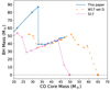 |
Fig. 17. Black hole mass spectrum as a function of the CO core mass from various authors. Solid blue line: this work, non-rotating progenitors at [Fe/H] =−3; long dashed orange line: set D of W17 (we note that these models are obtained from stellar tracks computed at Z = 0.1 Z⊙ for which the mass loss has been inhibited, making these models distinct from those we used to compute the final remnant masses.); dashed pink line: models from Spera & Mapelli (2017) with Z = 1.3 × 10⁻² Z⊙ (S17). Circles (crosses) represent the models that are stable (unstable) against pair production, and squares are the stars disrupted by PISNe. |
To compare the BH mass spectra, we choose the stellar tracks with zero initial angular velocities, to exclude the effects of chemical mixing and mass loss enhancement, and with the lowest initial metallicities, to exclude degeneracies caused by different stellar-wind models.
Figure 17 shows that the first progenitors that evolve through the pulsational pair-instability phase (marked with crosses) are those of S17, with a CO core mass of ∼24 M⊙. This happens because, to enter the PPISNe regime, S17 adopted the He core mass criterion proposed in W17 (He core mass of ∼32 M⊙), which corresponds to CO core masses of ∼24 M⊙ when used in combination with the S17 stellar evolution tracks from the PARSEC code (Bressan et al. 2012).
The tracks of W17 enter the PPISNe regime when the CO core mass is ∼28 M⊙. It is important to note that these stellar tracks were evolved suppressing the mass loss phenomena of a set of stars with initial metallicity of Z = 0.1 Z⊙, and that they were evolved from the ZAMS to the end of the PPISN regime. Thus, they represent a distinct set from the naked helium cores we used in Sects. 3.3 and 3.4 to infer the final remnant masses of the stars undergoing PPISNe.
Finally, our stellar progenitors become unstable against pair-instability when the CO core mass is ≳33 M⊙. From Figure 17 it is apparent that the BH maximum mass ranges from ∼87 M⊙ (this work) to the minimum value of ∼53 M⊙ (S17), resulting in a discrepancy of ∼38 M⊙ in the maximum mass of the BHs obtained by different authors from the evolution of an isolated massive star. The discrepancy exists because different authors have different thresholds in the CO core mass for entering the PPISNe regime (see also Farmer et al. 2019, hereinafter F19). For instance, if we had used the value of  from F19 (e.g.,
  ) we would have ended up with BHs more massive than ∼100 M⊙, i.e. in the regime of intermediate-mass BHs.
Figure 18 shows the BH mass spectrum of this work and the results we would obtain by applying the W17 and F19 criteria for the onset of PPISNe to the S17 stellar evolution tracks. It shows that even the progenitors from S17, which have the lowest PPISNe entry point ( ), can form BHs as massive as ∼70 M⊙ adopting the W17 threshold for the CO core mass (
 ) instead of the He core mass criterion. Furthermore, S17 can form BH as massive as ∼90 M⊙ adopting the F19 threshold (
 ), without changing the C/O ratio at the He core depletion, which is one of the key parameters to determine the onset of PPISNe (as shown in F19).
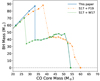 |
Fig. 18. Black hole mass spectrum as a function of the CO core mass for different PPISN prescriptions. Solid blue line: this work, non-rotating progenitors at [Fe/H] =−3; dash-dotted orange line: F19 PPISN threshold ( |

Therefore, adopting a self-consistent criterion to enter the PPISNe regime is crucial to investigate the BH mass spectrum and to constrain the lower edge of the upper mass gap. It is worth noting that the value of  is not the only property that affects the position of the lower edge of the upper mass gap. Besides the roles of DC, stellar winds, and rotation (cf. Sect. 3), the convective core overshooting parameter (αov) also has a central role in the formation of heavy stellar BHs. This is because overshooting dredges extra H from the envelope into the core during the central H burning; thus it governs the mass of the He core, and – in turn – the mass of the CO core. Vink et al. (2021) showed that a small value of overshooting (αov ≲ 0.1) is associated with smaller cores and stars likely end their life as Blue Super Giants (BSGs). Such stars are very compact, they tend to avoid the PPISNe regime, because they form smaller CO cores and they experience negligible mass loss during their life. As a consequence, such stars are likely to form very heavy BHs in the range 74–87 M⊙. In contrast, stars with higher values of αov exhibit more massive cores and likely evolve through the RSG phase, experiencing significant mass-loss episode. Hence, the stars enter the PPISNe with smaller pre-SN mass, forming less massive BHs.
We do not have conclusive evidence on the value of the core overshooting parameter yet, with observations providing evidence for higher possible values of the overshooting parameter than the one used in Vink et al. (2021; e.g., Vink et al. 2010; Brott et al. 2011; Higgins & Vink 2019; Bowman 2020; Sabhahit et al. 2023; Winch et al. 2024). Furthermore, other authors such as Takahashi (2018), Farmer et al. (2019), Farag et al. (2022), Mehta et al. (2022), and Shen et al. (2023) show that the variation in the C/O ratio at the He core depletion plays a role in the onset of the PPISNe.
The parameter space of the factors ruling the final fate of massive stars is still mostly unexplored, and from this analysis it is apparent that there is still room for many future improvements. We will explore the impact of these different effects on the onset of PPISNe in a follow-up work.
4.3. Remnants mass distribution
Figures 19 and 20 show the remnants mass distribution we obtain by evolving a population of 106 isolated single stars with an initial-mass function (IMF)  (Kroupa 2001) and MZAMS ∈ [15 M⊙;150 M⊙] for non-rotating and rotating progenitors, respectively. The mass of the remnant formed for each values of [Fe/H] and MZAMS is estimated by interpolating the MBH − MZAMS curve we find in Sects. 3.3, 3.4.
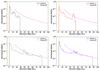 |
Fig. 19. Normalized probability distribution of BH masses we obtained from a population of 106 stars whose mass follows a Kroupa (2001) mass function (i.e., |
The panels of Figure 19 show several peaks in the remnants mass distribution. The most apparent peak of the remnants mass distributions is the one that corresponds to compact objects with mass 0.8–2 M⊙. This peak is a feature of the IMF and it shows up for all the considered metallicities for the non-rotating stars. It emerges because the majority of stellar progenitors extracted from the Kroupa IMF lie in the low-mass end with MZAMS ∈ [15 M⊙;20 M⊙], and they are expected to form NSs, as result of successful ccSNe.
At [Fe/H] = 0 (the top right panel of Figure 19), we find two other peaks in the remnant mass distribution, at BH masses of ∼9–13 M⊙ and ∼23 M⊙. The first one shows up because the MBH − MZAMS curve flattens out for MZAMS ∈ [30;40] causing an accumulation of BHs at ∼13 M⊙ (see the top left panel of Figure 13). The peak at ∼23 M⊙ occurs at the transition from successfully exploding progenitors to those that directly collapse to BHs. The heaviest BHs we obtain have masses ≃28 M⊙, consistent with the results presented in Sect. 3.3. At [Fe/H] = −1 (top right panel of Figure 19) we find two peaks in the remnants mass distribution at ∼13 M⊙ and ∼37 − 43 M⊙. The former corresponds to a local flattening of the MBH − MZAMS curve in the region of progenitors with MZAMS = 30 − 40 M⊙, and the latter is a degenerate effect due to the combination of the local flattening of the MBH − MZAMS curve and to the effect of the onset of the PPISNe, which causes significant mass loss and produce BHs with mass ∼37 − 48 M⊙. Furthermore, at this value of metallicity the heaviest BH that forms has a mass ∼44 M⊙, in agreement with the results presented in Sects. 2.3, 3.3.
At [Fe/H] = −2 (bottom left panel of Figure 19), we find two peaks in the distribution for BHs with masses of ∼40 M⊙, which again corresponds to the piling-up of BHs we obtain from the PPISNe, and of ∼78 − 84 M⊙. This latter is the result of the piling-up of BHs from the stellar progenitors with MZAMS between 80 M⊙ and 87 M⊙ where the slope of the MBH − MZAMS curve decreases. Furthermore, the heaviest BHs that form have mass ∼83 M⊙.
As in the case [Fe/H] = −2, at [Fe/H] = −3 (bottom right panel of Figure 19) we find that BHs pile up at masses ∼40 − 43 M⊙ because of PPISNe. We find that above the threshold for DC, the BH mass distribution follows the IMF distribution, since stellar winds are quenched and stars directly collapse to BHs with mass equal to MZAMS.
In summary, the features emerging from the BH mass distribution significantly depend on the adopted model, including the prescriptions for the pulsational pair-instability, and the details of the SN explosion. Furthermore, we find that the peak in the probability distribution corresponding to the transition between ccSNe and DC overlaps with the peak due to the PPISNe for some metallicities (e.g., [Fe/H] = −1). Such peaks in the remnants mass distribution are not only uncertain and model dependent, but also degenerate with the details of the SN explosion mechanism.
From Figure 20 it is apparent that stellar rotation significantly affects the remnants mass distribution. The peak corresponding to stellar progenitors extracted from the low-mass end of the Kroupa IMF is now shifted to BH with masses ∼4 M⊙ for [Fe/H] = 0, −3 (upper left panel and bottom right panel of Figure 20, respectively) and ∼12 M⊙ for [Fe/H] = −1, −2 (upper right panel and bottom left panel of Figure 20, respectively). This effect is a degenerate feature of the abundance of stars with MZAMS = 15 − 20 M⊙ and the outcome of the SN explosions at different initial metallicities for these stellar progenitors (see Sect. 3.4). Thus, we find that rotating stellar progenitors cannot produce NSs. At [Fe/H] = 0, we find that the distribution has a peak corresponding to ∼8 M⊙, which is due to the local flattening of the MBH − MZAMS curve in the interval of MZAMS between 20 M⊙ and 25 M⊙. The heaviest BH we form at solar metallicity has mass ∼19 M⊙.
At [Fe/H] = −2 we find a peak in the remnants mass distribution corresponding to BHs masses of ∼40 M⊙. This peak comes from the onset of the PPISNe. Such feature is independent of the details of the SN explosion and depends only on the prescription for the results of the PPISNe (combination of LC18 and W17 in this work). At [Fe/H] = −3, we find a peak in the remnants mass distribution, which corresponds to BH masses of ∼13 − 20 M⊙. The piling-up of BHs in this mass region is due to the particular shape of the MBH − MZAMS curve in the region of MZAMS between 15 M⊙ and ∼30 − 40 M⊙. In such region, the MBH − MZAMS curve has a local minimum at MZAMS = 25 M⊙, which produce a BH with mass ∼13 M⊙. Thus, a wide interval of progenitors piles-up BHs with mass in the interval ∼13 − 20 M⊙ (see also Figure 15). Furthermore, we find peaks in the remnant mass distribution corresponding to BH masses of ∼40 M⊙ ∼ 43 M⊙ and ∼47 M⊙. The first peak is a degenerate feature from both the SN explosion details and the prescriptions for the PPISNe. The latter two depend only on the MZAMS − Mrem curve we assume for the PPISNe. Finally, it is worth stressing that our results are based only on isolated single stars. Thus, considering binary stellar systems may significantly affects the results one can found about the BH mass spectrum.
4.4. Prescriptions for population synthesis codes
In this section, we present a set of analytic prescriptions derived from our results. Such fitting formulae can be implemented in population-synthesis models to calculate the mass of the remnants, given the physical properties of the progenitor at the pre-SN stage. The main value that our prescriptions provide is the fraction of mass that falls back onto the compact remnant during the explosion dM/M, that is
 (13)
(13)
with Mrem as the final remnant mass we obtain from the explosion.
The fraction of ejected mass is parametrized as a function of either the absolute value of the total energy, the binding energy of the stellar progenitor, or the CO core mass at the pre-SN stage. The total energy is computed as
 (14)
(14)
where Ebind is the binding energy of the whole progenitor, Eint is the internal energy and Ekin is the kinetic energy of the stellar matter, over the whole progenitor.
The panels of Figure 21 show the linear fit we obtain for the non-rotating (left panels) and the rotating progenitors (right panels), as a function of the absolute value of the total energy (top), binding energy (middle), and CO core mass (bottom). For such analysis, we studied the fate of the explosion independently of the initial metallicity, and thus in each panel we have all the models with [Fe/H] = 0 −1, −2, −3.
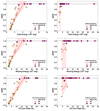 |
Fig. 21. Linear relation between the mass that falls back after the explosions and some structural properties of the stellar progenitors at the pre-SN stage, such as the absolute value of the total energy (top panels), the binding energy (central panels), and the CO core mass (bottom panels). We have performed such analysis both for the non-rotating (left panels) and for the rotating stellar progenitors (right panels). We studied the fate of the explosion independently of the initial metallicity. Thus, in each panel we have all the models with [Fe/H] = 0 −1, −2, −3. In each panel the circular orange points are the stellar progenitors undergoing successful SN explosions and the best fit for dM/M is the solid red line, while the diamond purple points represents the progenitors which DC to BHs. The black dashed line corresponds to dM/M = 1 i.e., the value of dM/M for the DC. The red shaded area is the 95% confidence interval for the SN linear regression. |
We first considered non-rotating progenitor models. We find that we can fit the relation between dM/M and the absolute value of the total energy as:
 (15)
(15)
with aSN = 0.26 foe−1, and bSN = −0.11, and |Etot|DC = 4.17 foe. The latter is the value of |Etot| for which dM/M = 0, i.e. for the DC.
From the top-left panel of Figure 21 it is apparent that two progenitors deviate significantly from our best fit. We find one stellar progenitor that directly collapses to BH despite having |Etot| < |Etot|DC, and one progenitor that explodes with |Etot| > |Etot|DC. The former star has MZAMS = 60 M⊙ and [Fe/H] = 0 and ends its life as a He-star, while the latter has MZAMS = 60 M⊙ and [Fe/H] = −1, and ends its life as a RSG, and therefore its H envelope is very loosely bound despite the high absolute value of the total energy. The relation between dM/M and the binding energy Ebind can be fit as:
 (16)
(16)
with cSN = 0.06 foe−1, and dSN = 0.04, and Ebind,DC = 15.9 foe.
From the central-left panel of Figure 21 it is apparent that one progenitor deviates significantly from the best fit. This is again the model with [Fe/H] = −1 and MZAMS = 60 M⊙, which explode as a SN with a binding energy of Ebind = 19.5 foe. If we did not consider this stellar progenitor, we would find a threshold value of ∼ 10.0 foe for the binding energy above which the stars DC to BHs.
Finally, the relation between dM/M and the CO core mass MCO can be fit as:
 (17)
(17)
with  , and fSN = −0.03, and
  , where again we find that only the two progenitor stars with MZAMS = 60 M⊙, [Fe/H] = −1 (that explodes as a SN despite having MCO = 21.4 M⊙ > MCO, DC), and with MZAMS = 60 M⊙, [Fe/H] = 0 (the He-star with MCO = 16.6 M⊙ < MCO, DC that directly collapses into a BH) deviate from the global trend.
In contrast, the right panels of Figure 21 show that rotating progenitors do not follow a linear relation between dM/M and |Etot|, Ebind, or MCO, and that there are no threshold values of any of these quantities that clearly separate stars which explode as SNe from stars which DC to BHs. Therefore, we cannot find any linear relation between the properties of rotating stars at the pre-SN stage and the final-remnant mass.
It is important to stress that – even in the case of non-rotating stellar progenitors – we can only provide a rough estimate of the thresholds for the transition from stars that successfully explode as ccSNe and stars that directly collapse to BH. From the left panels of Figure 21, it is apparent that a linear relation is in place below the threshold for the DC, but that some stars deviate from the expected trends, indicating that this approach fails to fully capture the complexity of a SN explosion. Our analysis shows that the fate of the collapse of each stellar progenitor is ruled only by the dynamics of the shock wave, i.e. the micro-physics effects taking place during the explosion are crucial in determining its outcome.
5. Summary and conclusion
In this paper, we studied the explosion of a subset of pre-SN models of massive stars presented in Limongi & Chieffi (2018). The subset contains massive stars with masses in the range 13 − 120 M⊙, initial metallicities [Fe/H] = 0, −1, −2, −3, and initial rotation velocities v = 0 km s−1, 300 km s−1. Using the HYPERION code (Limongi & Chieffi 2020), we simulate the explosion by removing the inner 0.8 M⊙ of the iron core, and injecting a given amount of thermal energy at the edge of this zone. Such approach required a set of free parameters to model the injection of energy. To fix these parameters, we have performed several calibration runs of a stellar progenitor similar to the progenitor of SN 1987A (Sk – 69°202), aimed at reproducing the observed kinetic energy of the ejecta (∼ 1.0 foe) and 56Ni mass (∼0.07 M⊙) (Arnett et al. 1989; Utrobin 1993, 2005, 2006; Blinnikov et al. 2000; Shigeyama & Nomoto 1990).
Once we have chosen the explosion parameters, we have adopted this combination for the explosion of all the models of our grid of stellar progenitor, obtaining both successful and failed explosions (DC to BHs), depending on the initial stellar parameters, i.e. mass, metallicity and rotation velocity.
We find that:
-
The metallicity plays a crucial role in the pre-SN evolution of a star, since it is strongly connected with the efficiency of stellar winds. For non-rotating models, progenitors with [Fe/H] = −2 and [Fe/H] = −3 evolve at roughly constant mass during their life, while for [Fe/H] = 0 and [Fe/H] = −1 the stellar winds remove a significant fraction of mass from the stellar progenitor. For these models we find that the threshold masses above which the stars undergo a DC to BH are MZAMS ≃ 60 M⊙ for [Fe/H] = 0, −2, −3 and MZAMS ≃ 80 M⊙ for [Fe/H] = −1. The most massive BH has mass of ≃91 M⊙, and comes from the DC of the most massive star at [Fe/H] = −3 not undergoing PPISNe (assuming that
 , see below).
 -
The presence of an initial angular rotation enhances the mass loss, and induces the formation of larger convective regions, and therefore larger CO cores (i.e., more bound structures). Thus, we find that for rotating stellar progenitors, the transition from a successful SN explosion to a DC to BHs occurs at lower MZAMS values (∼20 M⊙, ∼30 M⊙, ∼15 M⊙, and ∼20 M⊙, for [Fe/H] = 0, [Fe/H] = −1, [Fe/H] = −2, and [Fe/H] = −3, respectively) than for the non-rotating progenitors. In contrast, because of the enhanced mass loss driven by rotation, even if more stars DC to BHs, the maximum BH masses formed are lower than for non-rotating stars. In addition, the chemical mixing induces the onset of the PPISNe at lower values of MZAMS with respect to the non-rotating progenitors. As a result, the maximum BH mass formed by rotating progenitors is ∼41 M⊙, which comes from the DC of a stellar progenitors undergoing PPISNe, that we model according to the results of W17 (assuming that
 , see below).
 -
The maximum BH mass formed is very sensitive to the adopted criterium for the onset of PPISNe, which can be expressed in terms of the maximum CO core mass above which stars enter the PPISN regime,
 . From our simulated grid we find that
  , which is consistent with most of the published results. However, these vary considerably, from the lowest value adopted by S17,
  , to the highest value adopted by F19,
  . Such a discrepancy results in a significant uncertainty on the maximum BH mass, which can be as low as ∼53 M⊙ in the case of S17, or even as high as ∼87 M⊙, which is the case of this paper.
 -
We have applied the results of our simulations to a populations of 106 stars whose masses are distributed accordingly to a Kroupa-IMF. The resulting BH probability distribution depends on the initial stellar metallicity and rotation rate, and encode information on the progenitor mass – BH mass relation. We showed that the features emerging in the BH mass distribution depend significantly on the adopted stellar models and show significant degeneracies.
-
We provide linear relationships between the mass ejected during the explosion dM/M and the structural properties of the stellar progenitors at the pre-SN stage, such as the binding energy, the CO core mass and the absolute value of the total energy. Such relationships have been found only in the case of non-rotating stellar progenitors, even if some stars deviates from the linear fit. In contrast, we do not find any monotonic relationship between dM/M and the progenitor’s properties in the case of rotating stellar progenitors. We showed that, despite the relations can be adopted for fast population-synthesis studies, they fail to capture the details of the link between progenitor stars and their compact remnants.
It is worth mentioning that in this work we calibrate the explosions on the observational properties of SN1987A (i.e. the kinetic energy of the ejecta, and the mass of 56Ni ejected into the interstellar medium). In a follow-up study, we will broaden the set of SNe used for the calibration process.
Furthermore, we plan to increase the resolution in our grid of stellar progenitors in terms of MZAMS, initial metallicity and initial angular rotation to produce self-consistent estimates of the remnant masses of a larger grid of pre-SN models.
Finally, we plan to develop a large set of look-up tables, including rotating progenitor stars, that can be implemented in rapid binary population synthesis codes (e.g., SEVN; Spera et al. 2015, 2019; Spera & Mapelli 2017; Iorio et al. 2023) to investigate the evolution of compact-object binaries and the implications on detectable gravitational-wave signals.
Acknowledgments
This work has been partially developed at The Unconventional Thinking Tank Conference 2022, which is supported by INAF. MS acknowledges financial support from Fondazione ICSC, Spoke 3 Astrophysics and Cosmos Observations. National Recovery and Resilience Plan (Piano Nazionale di Ripresa e Resilienza, PNRR) Project ID CN_00000013 “Italian Research Center on High-Performance Computing, Big Data and Quantum Computing” funded by MUR Missione 4 Componente 2 Investimento 1.4: Potenziamento strutture di ricerca e creazione di “campioni nazionali di R&S (M4C2-19 )” – Next Generation EU (NGEU), and from the program “Data Science methods for Multi-Messenger Astrophysics & Multi-Survey Cosmology” funded by the Italian Ministry of University and Research, Programmazione triennale 2021/2023 (DM n.2503 dd. 09/12/2019), Programma Congiunto Scuole. RS acknowledges support from the PRIN 2022 MUR project 2022CB3PJ3 – First Light And Galaxy aSsembly (FLAGS) funded by the European Union – Next Generation EU and from ICSC – Centro Nazionale di Ricerca in High Performance Computing, Big Data and Quantum Computing, funded by European Union – NextGenerationEU.
References
- Abbott, B. P., Abbott, R., Abbott, T. D., et al. 2016a, Phys. Rev. D, 93, 122004 [NASA ADS] [CrossRef] [Google Scholar]
- Abbott, B. P., Abbott, R., Abbott, T. D., et al. 2016b, Phys. Rev. Lett., 116, 061102 [Google Scholar]
- Abbott, B. P., Abbott, R., Abbott, T. D., et al. 2016c, ApJ, 818, L22 [Google Scholar]
- Abbott, B. P., Abbott, R., Abbott, T. D., et al. 2019, ApJ, 882, L24 [Google Scholar]
- Abbott, R., Abbott, T. D., Acernese, F., et al. 2023, Phys. Rev. X, 13, 041039 [Google Scholar]
- Abbott, R., Abbott, T. D., Acernese, F., et al. 2024, Phys. Rev. D, 109, 022001 [NASA ADS] [CrossRef] [Google Scholar]
- Agrawal, P., Hurley, J., Stevenson, S., Szécsi, D., & Flynn, C. 2020, MNRAS, 497, 4549 [NASA ADS] [CrossRef] [Google Scholar]
- Aguilera-Dena, D. R., Müller, B., Antoniadis, J., et al. 2023, A&A, 671, A134 [NASA ADS] [CrossRef] [EDP Sciences] [Google Scholar]
- Arnett, D., & Chevalier, R. 1996, Phys. Today, 49, 68 [NASA ADS] [CrossRef] [Google Scholar]
- Arnett, W. D., Bahcall, J. N., Kirshner, R. P., & Woosley, S. E. 1989, ARA&A, 27, 629 [NASA ADS] [CrossRef] [Google Scholar]
- Asplund, M., Grevesse, N., Sauval, A. J., & Scott, P. 2009, ARA&A, 47, 481 [NASA ADS] [CrossRef] [Google Scholar]
- Banerjee, S. 2017, MNRAS, 467, 524 [NASA ADS] [Google Scholar]
- Banerjee, S. 2018, MNRAS, 473, 909 [CrossRef] [Google Scholar]
- Banerjee, S. 2021, MNRAS, 500, 3002 [Google Scholar]
- Banerjee, S., Baumgardt, H., & Kroupa, P. 2010, MNRAS, 402, 371 [Google Scholar]
- Barkat, Z., Rakavy, G., & Sack, N. 1967, Phys. Rev. Lett., 18, 379 [Google Scholar]
- Belczynski, K., Holz, D. E., Bulik, T., & O’Shaughnessy, R. 2016, Nature, 534, 512 [NASA ADS] [CrossRef] [Google Scholar]
- Belczynski, K., Askar, A., Arca-Sedda, M., et al. 2018, A&A, 615, A91 [NASA ADS] [CrossRef] [EDP Sciences] [Google Scholar]
- Belczynski, K., Klencki, J., Fields, C. E., et al. 2020, A&A, 636, A104 [NASA ADS] [CrossRef] [EDP Sciences] [Google Scholar]
- Bersten, M. C., Benvenuto, O., & Hamuy, M. 2011, ApJ, 729, 61 [NASA ADS] [CrossRef] [Google Scholar]
- Bethe, H. A., & Brown, G. E. 1998, ApJ, 506, 780 [Google Scholar]
- Bethe, H. A., & Wilson, J. R. 1985, ApJ, 295, 14 [CrossRef] [Google Scholar]
- Blinnikov, S., Lundqvist, P., Bartunov, O., Nomoto, K., & Iwamoto, K. 2000, ApJ, 532, 1132 [NASA ADS] [CrossRef] [Google Scholar]
- Blondin, J. M., Mezzacappa, A., & DeMarino, C. 2003, ApJ, 584, 971 [NASA ADS] [CrossRef] [Google Scholar]
- Bollig, R., Yadav, N., Kresse, D., et al. 2021, ApJ, 915, 28 [NASA ADS] [CrossRef] [Google Scholar]
- Bowman, D. M. 2020, Front. Astron. Space Sci., 7, 70 [Google Scholar]
- Bressan, A., Marigo, P., Girardi, L., et al. 2012, MNRAS, 427, 127 [NASA ADS] [CrossRef] [Google Scholar]
- Broekgaarden, F. S., Berger, E., Neijssel, C. J., et al. 2021, MNRAS, 508, 5028 [NASA ADS] [CrossRef] [Google Scholar]
- Brott, I., de Mink, S. E., Cantiello, M., et al. 2011, A&A, 530, A115 [NASA ADS] [CrossRef] [EDP Sciences] [Google Scholar]
- Brown, G. E. 1995, ApJ, 440, 270 [NASA ADS] [CrossRef] [Google Scholar]
- Bruenn, S. W., Lentz, E. J., Hix, W. R., et al. 2016, ApJ, 818, 123 [Google Scholar]
- Burrows, A., Hayes, J., & Fryxell, B. A. 1995, ApJ, 450, 830 [NASA ADS] [CrossRef] [Google Scholar]
- Burrows, A., Radice, D., & Vartanyan, D. 2019, MNRAS, 485, 3153 [NASA ADS] [CrossRef] [Google Scholar]
- Burrows, A., Radice, D., Vartanyan, D., et al. 2020, MNRAS, 491, 2715 [NASA ADS] [CrossRef] [Google Scholar]
- Burrows, A., Vartanyan, D., & Wang, T. 2023a, ApJ, 957, 68 [NASA ADS] [CrossRef] [Google Scholar]
- Burrows, A., Wang, T., Vartanyan, D., & Coleman, M. S. B. 2023b, arXiv e-prints [arXiv:2311.12109] [Google Scholar]
- Cayrel, R., Depagne, E., Spite, M., et al. 2004, A&A, 416, 1117 [NASA ADS] [CrossRef] [EDP Sciences] [Google Scholar]
- Chaboyer, B., & Zahn, J. P. 1992, A&A, 253, 173 [NASA ADS] [Google Scholar]
- Chieffi, A., & Limongi, M. 2004, ApJ, 608, 405 [NASA ADS] [CrossRef] [Google Scholar]
- Chieffi, A., & Limongi, M. 2013, ApJ, 764, 21 [Google Scholar]
- Colella, P., & Woodward, P. R. 1984, J. Comput. Phys., 54, 174 [NASA ADS] [CrossRef] [Google Scholar]
- Costa, G., Bressan, A., Mapelli, M., et al. 2021, MNRAS, 501, 4514 [NASA ADS] [CrossRef] [Google Scholar]
- de Jager, C., Nieuwenhuijzen, H., & van der Hucht, K. A. 1988, A&AS, 72, 259 [NASA ADS] [Google Scholar]
- Dewi, J. D. M., Podsiadlowski, P., & Sena, A. 2006, MNRAS, 368, 1742 [NASA ADS] [CrossRef] [Google Scholar]
- Di Carlo, U. N., Giacobbo, N., Mapelli, M., et al. 2019, MNRAS, 487, 2947 [NASA ADS] [CrossRef] [Google Scholar]
- Di Carlo, U. N., Mapelli, M., Bouffanais, Y., et al. 2020a, MNRAS, 497, 1043 [NASA ADS] [CrossRef] [Google Scholar]
- Di Carlo, U. N., Mapelli, M., Giacobbo, N., et al. 2020b, MNRAS, 498, 495 [NASA ADS] [CrossRef] [Google Scholar]
- Di Carlo, U. N., Mapelli, M., Pasquato, M., et al. 2021, MNRAS, 507, 5132 [NASA ADS] [CrossRef] [Google Scholar]
- Doherty, C. L., Gil-Pons, P., Siess, L., & Lattanzio, J. C. 2017, PASA, 34 [CrossRef] [Google Scholar]
- Dominik, M., Belczynski, K., Fryer, C., et al. 2012, ApJ, 759, 52 [Google Scholar]
- Dominik, M., Berti, E., O’Shaughnessy, R., et al. 2015, ApJ, 806, 263 [Google Scholar]
- Downing, J. M. B., Benacquista, M. J., Giersz, M., & Spurzem, R. 2011, MNRAS, 416, 133 [Google Scholar]
- Eldridge, J. J., Izzard, R. G., & Tout, C. A. 2008, MNRAS, 384, 1109 [Google Scholar]
- Ertl, T., Janka, H. T., Woosley, S. E., Sukhbold, T., & Ugliano, M. 2016, ApJ, 818, 124 [NASA ADS] [CrossRef] [Google Scholar]
- Farag, E., Renzo, M., Farmer, R., Chidester, M. T., & Timmes, F. X. 2022, ApJ, 937, 112 [NASA ADS] [CrossRef] [Google Scholar]
- Farmer, R., Renzo, M., de Mink, S. E., Marchant, P., & Justham, S. 2019, ApJ, 887, 53 [Google Scholar]
- Ferguson, J. W., Alexander, D. R., Allard, F., et al. 2005, ApJ, 623, 585 [Google Scholar]
- Fernández, R., Quataert, E., Kashiyama, K., & Coughlin, E. R. 2018, MNRAS, 476, 2366 [CrossRef] [Google Scholar]
- Foglizzo, T., Scheck, L., & Janka, H.-T. 2006, ApJ, 652, 1436 [NASA ADS] [CrossRef] [Google Scholar]
- Fowler, W. A., & Hoyle, F. 1964, ApJS, 9, 201 [Google Scholar]
- Fragos, T., Andrews, J. J., Bavera, S. S., et al. 2023, ApJS, 264, 45 [NASA ADS] [CrossRef] [Google Scholar]
- Fryer, C. L., Belczynski, K., Wiktorowicz, G., et al. 2012, ApJ, 749, 91 [Google Scholar]
- Gallegos-Garcia, M., Berry, C. P. L., Marchant, P., & Kalogera, V. 2021, ApJ, 922, 110 [NASA ADS] [CrossRef] [Google Scholar]
- Graziani, L., Schneider, R., Marassi, S., et al. 2020, MNRAS, 495, L81 [NASA ADS] [CrossRef] [Google Scholar]
- Hashimoto, M., Nomoto, K., & Shigeyama, T. 1989, A&A, 210, L5 [NASA ADS] [Google Scholar]
- Heger, A., & Langer, N. 2000, ApJ, 544, 1016 [CrossRef] [Google Scholar]
- Heger, A., & Woosley, S. E. 2002, ApJ, 567, 532 [Google Scholar]
- Heggie, D. C. 1975, MNRAS, 173, 729 [NASA ADS] [CrossRef] [Google Scholar]
- Herant, M., Benz, W., Hix, W. R., Fryer, C. L., & Colgate, S. A. 1994, ApJ, 435, 339 [NASA ADS] [CrossRef] [Google Scholar]
- Higgins, E. R., & Vink, J. S. 2019, A&A, 622, A50 [NASA ADS] [CrossRef] [EDP Sciences] [Google Scholar]
- Horiuchi, S., Nakamura, K., Takiwaki, T., Kotake, K., & Tanaka, M. 2014, MNRAS, 445, L99 [NASA ADS] [CrossRef] [Google Scholar]
- Huebner, W., Merts, A., Magee, N., & Argo, Jr., M. 1977, Los Alamos Scientific Laboratory Report [Google Scholar]
- Iglesias, C. A., & Rogers, F. J. 1996, ApJ, 464, 943 [NASA ADS] [CrossRef] [Google Scholar]
- Iglesias, C. A., Rogers, F. J., & Wilson, B. G. 1992, ApJ, 397, 717 [NASA ADS] [CrossRef] [Google Scholar]
- Iorio, G., Mapelli, M., Costa, G., et al. 2023, MNRAS, 524, 426 [NASA ADS] [CrossRef] [Google Scholar]
- Itoh, N., Mitake, S., Iyetomi, H., & Ichimaru, S. 1983, ApJ, 273, 774 [NASA ADS] [CrossRef] [Google Scholar]
- Janka, H. T. 2017, in Handbook of Supernovae, eds. A. W. Alsabti, & P. Murdin, 1095 [CrossRef] [Google Scholar]
- Janka, H. T., & Mueller, E. 1996, A&A, 306, 167 [NASA ADS] [Google Scholar]
- Janka, H.-T., Melson, T., & Summa, A. 2016, Annu. Rev. Nucl. Part. Sci., 66, 341 [Google Scholar]
- Justham, S., Podsiadlowski, P., & Han, Z. 2011, MNRAS, 410, 984 [CrossRef] [Google Scholar]
- Kinugawa, T., Nakamura, T., & Nakano, H. 2021, MNRAS, 501, L49 [Google Scholar]
- Kinugawa, T., Horiuchi, S., Takiwaki, T., & Kotake, K. 2024, MNRAS, 532, 3926 [NASA ADS] [CrossRef] [Google Scholar]
- Kotake, K., Sato, K., & Takahashi, K. 2006, Rep. Prog. Phys., 69, 971 [NASA ADS] [CrossRef] [Google Scholar]
- Kremer, K., Ye, C. S., Rui, N. Z., et al. 2020, ApJS, 247, 48 [NASA ADS] [CrossRef] [Google Scholar]
- Kroupa, P. 2001, MNRAS, 322, 231 [NASA ADS] [CrossRef] [Google Scholar]
- Kurucz, R. L. 1991, in Stellar Atmospheres - Beyond Classical Models, eds. L. Crivellari, I. Hubeny, & D. G. Hummer, NATO ASI Ser. C, 341, 441 [NASA ADS] [CrossRef] [Google Scholar]
- Lentz, E. J., Mezzacappa, A., Messer, O. E. B., et al. 2012, ApJ, 747, 73 [NASA ADS] [CrossRef] [Google Scholar]
- Lentz, E. J., Bruenn, S. W., Hix, W. R., et al. 2015, ApJ, 807, L31 [NASA ADS] [CrossRef] [Google Scholar]
- Levermore, C. D., & Pomraning, G. C. 1981, ApJ, 248, 321 [NASA ADS] [CrossRef] [Google Scholar]
- Limongi, M., & Chieffi, A. 2003, ApJ, 592, 404 [CrossRef] [Google Scholar]
- Limongi, M., & Chieffi, A. 2006, ApJ, 647, 483 [NASA ADS] [CrossRef] [Google Scholar]
- Limongi, M., & Chieffi, A. 2018, ApJS, 237, 13 [NASA ADS] [CrossRef] [Google Scholar]
- Limongi, M., & Chieffi, A. 2020, ApJ, 902, 95 [NASA ADS] [CrossRef] [Google Scholar]
- Limongi, M., Straniero, O., & Chieffi, A. 2000, ApJS, 129, 625 [NASA ADS] [CrossRef] [Google Scholar]
- Lovegrove, E., & Woosley, S. E. 2013, ApJ, 769, 109 [NASA ADS] [CrossRef] [Google Scholar]
- Maeder, A., & Zahn, J.-P. 1998, A&A, 334, 1000 [NASA ADS] [Google Scholar]
- Mandel, I., & Farmer, A. 2022, Phys. Rep., 955, 1 [NASA ADS] [CrossRef] [Google Scholar]
- Mandel, I., & Fragos, T. 2020, ApJ, 895, L28 [Google Scholar]
- Mandel, I., & Müller, B. 2020, MNRAS, 499, 3214 [NASA ADS] [CrossRef] [Google Scholar]
- Mapelli, M. 2016, MNRAS, 459, 3432 [NASA ADS] [CrossRef] [Google Scholar]
- Mapelli, M. 2021, Handbook of Gravitational Wave Astronomy, 16 (Springer) [Google Scholar]
- Mapelli, M., & Giacobbo, N. 2018, MNRAS, 479, 4391 [NASA ADS] [CrossRef] [Google Scholar]
- Mapelli, M., Zampieri, L., Ripamonti, E., & Bressan, A. 2013, MNRAS, 429, 2298 [NASA ADS] [CrossRef] [Google Scholar]
- Mapelli, M., Spera, M., Montanari, E., et al. 2020, ApJ, 888, 76 [NASA ADS] [CrossRef] [Google Scholar]
- Marassi, S., Graziani, L., Ginolfi, M., et al. 2019a, MNRAS, 484, 3219 [NASA ADS] [CrossRef] [Google Scholar]
- Marassi, S., Schneider, R., Limongi, M., et al. 2019b, MNRAS, 484, 2587 [NASA ADS] [CrossRef] [Google Scholar]
- Marchant, P., Pappas, K. M. W., Gallegos-Garcia, M., et al. 2021, A&A, 650, A107 [NASA ADS] [CrossRef] [EDP Sciences] [Google Scholar]
- Mehta, A. K., Buonanno, A., Gair, J., et al. 2022, ApJ, 924, 39 [CrossRef] [Google Scholar]
- Menon, A., & Heger, A. 2017, MNRAS, 469, 4649 [NASA ADS] [Google Scholar]
- Meynet, G., & Maeder, A. 1997, A&A, 321, 465 [NASA ADS] [Google Scholar]
- Meynet, G., & Maeder, A. 2000, A&A, 361, 101 [NASA ADS] [Google Scholar]
- Mezzacappa, A., Endeve, E., Messer, O. E. B., & Bruenn, S. W. 2020, Liv. Rev. Comput. Astrophys., 6, 4 [CrossRef] [Google Scholar]
- Mezzacappa, A., Marronetti, P., Landfield, R. E., et al. 2023, Phys. Rev. D, 107, 043008 [NASA ADS] [CrossRef] [Google Scholar]
- Miller-Jones, J. C. A., Bahramian, A., Orosz, J. A., et al. 2021, Science, 371, 1046 [Google Scholar]
- Moody, K., & Sigurdsson, S. 2009, ApJ, 690, 1370 [NASA ADS] [CrossRef] [Google Scholar]
- Moriya, T., Tominaga, N., Tanaka, M., et al. 2010, ApJ, 719, 1445 [NASA ADS] [CrossRef] [Google Scholar]
- Morozova, V., Piro, A. L., Renzo, M., et al. 2015, ApJ, 814, 63 [Google Scholar]
- Müller, B. 2015, MNRAS, 453, 287 [CrossRef] [Google Scholar]
- Müller, B., Janka, H.-T., & Heger, A. 2012, ApJ, 761, 72 [CrossRef] [Google Scholar]
- Nadezhin, D. K. 1980, Ap&SS, 69, 115 [NASA ADS] [CrossRef] [Google Scholar]
- Nakamura, T., Umeda, H., Iwamoto, K., et al. 2001, ApJ, 555, 880 [NASA ADS] [CrossRef] [Google Scholar]
- Nakamura, K., Takiwaki, T., Matsumoto, J., & Kotake, K. 2025, MNRAS, 536, 280 [Google Scholar]
- Neijssel, C. J., Vigna-Gómez, A., Stevenson, S., et al. 2019, MNRAS, 490, 3740 [Google Scholar]
- Nomoto, K., Tominaga, N., Umeda, H., Kobayashi, C., & Maeda, K. 2006, Nucl. Phys. A, 777, 424 [CrossRef] [Google Scholar]
- Nugis, T., & Lamers, H. J. G. L. M. 2000, A&A, 360, 227 [NASA ADS] [Google Scholar]
- O’Connor, E., & Ott, C. D. 2011, ApJ, 730, 70 [Google Scholar]
- Orosz, J. A. 2003, IAU Symp., 212, 365 [NASA ADS] [Google Scholar]
- Özel, F., Psaltis, D., Narayan, R., & McClintock, J. E. 2010, ApJ, 725, 1918 [CrossRef] [Google Scholar]
- Paczynski, B. 1983, ApJ, 267, 315 [CrossRef] [Google Scholar]
- Palacios, A., Talon, S., Charbonnel, C., & Forestini, M. 2003, A&A, 399, 603 [CrossRef] [EDP Sciences] [Google Scholar]
- Patton, R. A., & Sukhbold, T. 2020, MNRAS, 499, 2803 [NASA ADS] [CrossRef] [Google Scholar]
- Patton, R. A., Sukhbold, T., & Eldridge, J. J. 2022, MNRAS, 511, 903 [NASA ADS] [CrossRef] [Google Scholar]
- Pavlovskii, K., Ivanova, N., Belczynski, K., & Van, K. X. 2017, MNRAS, 465, 2092 [Google Scholar]
- Piro, A. L. 2013, ApJ, 768, L14 [NASA ADS] [CrossRef] [Google Scholar]
- Podsiadlowski, P. 1992, PASP, 104, 717 [CrossRef] [Google Scholar]
- Poelarends, A. J. T., Wurtz, S., Tarka, J., Cole Adams, L., & Hills, S. T. 2017, ApJ, 850, 197 [NASA ADS] [CrossRef] [Google Scholar]
- Powell, J., Müller, B., Aguilera-Dena, D. R., & Langer, N. 2023, MNRAS, 522, 6070 [NASA ADS] [CrossRef] [Google Scholar]
- Rakavy, G., & Shaviv, G. 1967, ApJ, 148, 803 [Google Scholar]
- Rastello, S., Amaro-Seoane, P., Arca-Sedda, M., et al. 2019, MNRAS, 483, 1233 [NASA ADS] [CrossRef] [Google Scholar]
- Rastello, S., Mapelli, M., Di Carlo, U. N., et al. 2020, MNRAS, 497, 1563 [CrossRef] [Google Scholar]
- Rastello, S., Mapelli, M., Di Carlo, U. N., et al. 2021, MNRAS, 507, 3612 [CrossRef] [Google Scholar]
- Roberti, L., Limongi, M., & Chieffi, A. 2024, ApJS, 270, 28 [NASA ADS] [CrossRef] [Google Scholar]
- Rodriguez, C. L., Morscher, M., Pattabiraman, B., et al. 2015, Phys. Rev. Lett., 115, 051101 [Google Scholar]
- Rodriguez, C. L., Haster, C.-J., Chatterjee, S., Kalogera, V., & Rasio, F. A. 2016, ApJ, 824, L8 [NASA ADS] [CrossRef] [Google Scholar]
- Rodriguez, C. L., Zevin, M., Amaro-Seoane, P., et al. 2019, Phys. Rev. D, 100, 043027 [Google Scholar]
- Rogers, F. J. 2001, Contrib. Plasma Phys., 41, 179 [NASA ADS] [CrossRef] [Google Scholar]
- Rogers, F. J., Swenson, F. J., & Iglesias, C. A. 1996, ApJ, 456, 902 [Google Scholar]
- Sabhahit, G. N., Vink, J. S., Sander, A. A. C., & Higgins, E. R. 2023, MNRAS, 524, 1529 [NASA ADS] [CrossRef] [Google Scholar]
- Sallaska, A. L., Iliadis, C., Champange, A. E., et al. 2013, ApJS, 207, 18 [Google Scholar]
- Sandquist, E. L., Taam, R. E., Chen, X., Bodenheimer, P., & Burkert, A. 1998, ApJ, 500, 909 [NASA ADS] [CrossRef] [Google Scholar]
- Schneider, F. R. N., Izzard, R. G., Langer, N., & de Mink, S. E. 2015, ApJ, 805, 20 [Google Scholar]
- Shen, Y., Guo, B., deBoer, R. J., et al. 2023, ApJ, 945, 41 [NASA ADS] [CrossRef] [Google Scholar]
- Shibagaki, S., Kuroda, T., Kotake, K., Takiwaki, T., & Fischer, T. 2024, MNRAS, 531, 3732 [NASA ADS] [CrossRef] [Google Scholar]
- Shigeyama, T., & Nomoto, K. 1990, ApJ, 360, 242 [CrossRef] [Google Scholar]
- Shigeyama, T., Nomoto, K., & Hashimoto, M. 1988, A&A, 196, 141 [NASA ADS] [Google Scholar]
- Sigurdsson, S., & Hernquist, L. 1993, Nature, 364, 423 [Google Scholar]
- Sigurdsson, S., & Phinney, E. S. 1995, ApJS, 99, 609 [NASA ADS] [CrossRef] [Google Scholar]
- Spera, M., & Mapelli, M. 2017, MNRAS, 470, 4739 [Google Scholar]
- Spera, M., Mapelli, M., & Bressan, A. 2015, MNRAS, 451, 4086 [NASA ADS] [CrossRef] [Google Scholar]
- Spera, M., Mapelli, M., Giacobbo, N., et al. 2019, MNRAS, 485, 889 [Google Scholar]
- Spera, M., Trani, A. A., & Mencagli, M. 2022, Galaxies, 10, 76 [NASA ADS] [CrossRef] [Google Scholar]
- Spite, M., Cayrel, R., Plez, B., et al. 2005, A&A, 430, 655 [NASA ADS] [CrossRef] [EDP Sciences] [Google Scholar]
- Straniero, O. 1988, A&AS, 76, 157 [NASA ADS] [Google Scholar]
- Sukhbold, T., Ertl, T., Woosley, S. E., Brown, J. M., & Janka, H.-T. 2016, ApJ, 821, 38 [Google Scholar]
- Sukhbold, T., Woosley, S. E., & Heger, A. 2018, ApJ, 860, 93 [NASA ADS] [CrossRef] [Google Scholar]
- Summa, A., Hanke, F., Janka, H.-T., et al. 2016, ApJ, 825, 6 [NASA ADS] [CrossRef] [Google Scholar]
- Suwa, Y., Kotake, K., Takiwaki, T., et al. 2010, PASJ, 62, L49 [NASA ADS] [CrossRef] [Google Scholar]
- Suwa, Y., Takiwaki, T., Kotake, K., et al. 2013, ApJ, 764, 99 [CrossRef] [Google Scholar]
- Swartz, D. A., Sutherland, P. G., & Harkness, R. P. 1995, ApJ, 446, 766 [NASA ADS] [CrossRef] [Google Scholar]
- Takahashi, K. 2018, ApJ, 863, 153 [Google Scholar]
- Talon, S., & Zahn, J. P. 1997, A&A, 317, 749 [NASA ADS] [Google Scholar]
- Thielemann, F.-K., Hashimoto, M.-A., & Nomoto, K. 1990, ApJ, 349, 222 [CrossRef] [Google Scholar]
- Thielemann, F.-K., Nomoto, K., & Hashimoto, M.-A. 1996, ApJ, 460, 408 [NASA ADS] [CrossRef] [Google Scholar]
- Tutukov, A. V., & Yungelson, L. R. 1993, MNRAS, 260, 675 [Google Scholar]
- Ugliano, M., Janka, H.-T., Marek, A., & Arcones, A. 2012, ApJ, 757, 69 [NASA ADS] [CrossRef] [Google Scholar]
- Umeda, H., & Nomoto, K. 2008, ApJ, 673, 1014 [NASA ADS] [CrossRef] [Google Scholar]
- Utrobin, V. 1993, A&A, 270, 249 [NASA ADS] [Google Scholar]
- Utrobin, V. P. 2005, Astron. Lett., 31, 806 [NASA ADS] [CrossRef] [Google Scholar]
- Utrobin, V. P. 2006, A&A, 461, 233 [Google Scholar]
- van den Heuvel, E. P. J., & De Loore, C. 1973, A&A, 25, 387 [NASA ADS] [Google Scholar]
- van den Heuvel, E. P. J., Portegies Zwart, S. F., & de Mink, S. E. 2017, MNRAS, 471, 4256 [Google Scholar]
- van Loon, J. T., Cioni, M. R. L., Zijlstra, A. A., & Loup, C. 2005, A&A, 438, 273 [NASA ADS] [CrossRef] [EDP Sciences] [Google Scholar]
- van Son, L. A. C., De Mink, S. E., Broekgaarden, F. S., et al. 2020, ApJ, 897, 100 [Google Scholar]
- Vartanyan, D., Burrows, A., Wang, T., Coleman, M. S. B., & White, C. J. 2023, Phys. Rev. D, 107, 103015 [NASA ADS] [CrossRef] [Google Scholar]
- Vigna-Gómez, A., Neijssel, C. J., Stevenson, S., et al. 2018, MNRAS, 481, 4009 [Google Scholar]
- Vink, J. S., de Koter, A., & Lamers, H. J. G. L. M. 2000, A&A, 362, 295 [Google Scholar]
- Vink, J. S., de Koter, A., & Lamers, H. J. G. L. M. 2001, A&A, 369, 574 [NASA ADS] [CrossRef] [EDP Sciences] [Google Scholar]
- Vink, J. S., Brott, I., Gräfener, G., et al. 2010, A&A, 512, L7 [NASA ADS] [CrossRef] [EDP Sciences] [Google Scholar]
- Vink, J. S., Higgins, E. R., Sander, A. A. C., & Sabhahit, G. N. 2021, MNRAS, 504, 146 [NASA ADS] [CrossRef] [Google Scholar]
- Wang, L. 2020, MNRAS, 491, 2413 [NASA ADS] [Google Scholar]
- Wang, L., Tanikawa, A., & Fujii, M. 2022, MNRAS, 515, 5106 [NASA ADS] [CrossRef] [Google Scholar]
- Winch, E. R. J., Vink, J. S., Higgins, E. R., & Sabhahitf, G. N. 2024, MNRAS, 529, 2980 [NASA ADS] [CrossRef] [Google Scholar]
- Woosley, S. E. 1988, ApJ, 330, 218 [Google Scholar]
- Woosley, S. E. 2017, ApJ, 836, 244 [Google Scholar]
- Woosley, S. E., & Weaver, T. A. 1995, ApJS, 101, 181 [Google Scholar]
- Wysocki, D., Gerosa, D., O’Shaughnessy, R., et al. 2018, Phys. Rev. D, 97, 043014 [NASA ADS] [CrossRef] [Google Scholar]
- Ye, C. S., Kremer, K., Rodriguez, C. L., et al. 2022, ApJ, 931, 84 [NASA ADS] [CrossRef] [Google Scholar]
- Zaghloul, M. R., Bourham, M. A., & Doster, J. M. 2000, J. Phys. D: Appl. Phys., 33, 977 [NASA ADS] [CrossRef] [Google Scholar]
- Zahn, J. P. 1992, A&A, 265, 115 [NASA ADS] [Google Scholar]
- Zapartas, E., de Mink, S. E., Izzard, R. G., et al. 2017, A&A, 601, A29 [NASA ADS] [CrossRef] [EDP Sciences] [Google Scholar]
- Zapartas, E., Renzo, M., Fragos, T., et al. 2021, A&A, 656, L19 [NASA ADS] [CrossRef] [EDP Sciences] [Google Scholar]
- Zevin, M., Bavera, S. S., Berry, C. P. L., et al. 2021, ApJ, 910, 152 [Google Scholar]
- Ziosi, B. M., Mapelli, M., Branchesi, M., & Tormen, G. 2014, MNRAS, 441, 3703 [Google Scholar]
Appendix A: The FRANEC code
In this Appendix, we summarize the main features of the FRANEC stellar evolutionary code. For a complete description, we refer the reader to Chieffi & Limongi (2013) and Limongi & Chieffi (2018).
The FRANEC code couples all the equations describing the physical structure of the star and the chemical evolution of the matted due to both the nuclear ractions and the various mixing processes (convection, rotation, diffusion, semiconvectionm etc.) and solves them simultaneously by using a relaxation technique.
Convective envelope boundaries are determined using the Ledoux criterion, and an overshooting of 0.2Hp is included at the convective core’s outer edge during the core hydrogen-burning phase.
The equation of state (EoS) provided by Rogers et al. (1996), Rogers (2001) (EOS and EOSPLUS) is adopted for temperatures below 106 K while the EoS provided by Straniero (1988) is used for temperatures T ≥ 106 K. Radiative opacity coefficients are derived from Kurucz (1991) for T ≤ 104 K, Iglesias et al. (1992) (OPAL) and the Los Alamos Opacity Library (LAOL) Huebner et al. (1977) for 104 K < T ≤ 108 K, and T ≥ 108 K, respectively. Thermal conductivity opacity coefficients follow Itoh et al. (1983).
Stellar wind mass loss is implemented according to Vink et al. (2000, 2001) for the blue supergiant (BSG) phase (Teff ≥ 1.2 × 10⁴ K), de Jager et al. (1988) for the red supergiant (RSG) phase (Teff < 1.2 × 10⁴ K), and Nugis & Lamers (2000) for the Wolf-Rayet (WR) phase. For stars in the RSG phase, dust-enhanced stellar winds are included following van Loon et al. (2005). In rotating models, mass loss is enhanced according to Heger & Langer (2000).
The classification criteria for WR subclasses follow Limongi & Chieffi (2006):
-
WNL: 10−5 < Hsurf < 0.4,
-
WNE: Hsurf < 10−5 and (C/N)surf < 0.1,
-
WNC: 0.1 < (C/N)surf < 10,
-
WCO: (C/N)surf > 10.
The nuclear network used in LC18 includes 335 isotopes, ranging from neutrons to Bi209, as detailed in Table 1 of LC18. For isotopes near the magic numbers N = 82 and N = 126, only neutron captures and beta decays are explicitly followed, while intermediate isotopes are assumed to be in local equilibrium. This approach ensures computational efficiency without compromising accuracy, as validated by one-zone core helium burning calculations comparing the full network to an extended one, both yielding consistent abundances around A = 131 − 145.
Nuclear cross-sections and weak interaction rates in LC18 are updated with respect to Chieffi & Limongi (2013), when possible, using the latest data. Most of the nuclear rates are extracted from the STARLIB database Sallaska et al. (2013), with Tables 3 and 4 of LC18 providing a full reference matrix of all the processes included in the network along with their proper legend.
The effect of rotation on stellar structure is modeled using the “shellular rotation” approach (Zahn 1992; Meynet & Maeder 1997). Angular momentum transport due to meridional circulation and shear turbulence is computed via an advective-diffusive equation Chaboyer & Zahn (1992), Talon & Zahn (1997):
 (A.1)
(A.1)
where U is the radial velocity from meridional circulation, Ds.i. is the shear turbulence diffusion coefficient, ω is angular rotation, ρ is density, and r is radius. Prescriptions for U are from Maeder & Zahn (1998), and Ds.i. follows Palacios et al. (2003):
 (A.2)
(A.2)
where  ,
,  ,
,  . Dh = |rU| is horizontal turbulence (Zahn 1992), and K is thermal diffusivity (Meynet & Maeder 2000).
The adoption of the meridional circulation velocity provided by Maeder & Zahn (1998) transforms equation A.1 into a fourth-order partial differential equation, that FRANEC solves with a relaxation technique.
Rotation driven mixing is treated as a purely diffusive process (Chaboyer & Zahn 1992). The diffusion coefficient is given by:
 (A.3)
(A.3)
where Dm.c. = |rU|2/(30Dh) (Zahn 1992). Calibration parameters fc and fμ adjust mixing and weight the molecular weight gradient. These calibrations are detailed in LC18.
Finally, the initial helium abundance and mixing-length parameters are calibrated to match the Sun’s present-day properties.
Appendix B: Calibration parameters
In Sec.2.2 we present the calibration of our parameters and the final set we choose to stimulate the SN explosion in our simulations. In this Appendix we further discuss the contribution of the different parameters Einj, dminj and dtinj.
B.1. Calibration of Einj
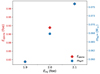 |
Fig. B.1. Values of Eejecta (red diamonds, whose scale is on the left-hand y-axes) and m56Ni (blue points, whose scale is on the right-hand y-axis) as function of Einj. |
Figure B.1 shows the values that we find for Eejecta and m56Ni for different values of Einj. We studied the variation of the outcomes of the explosion assuming dtinj = 10−9s and dminj = 0.1M⊙, and by injecting the thermal energy at the arbitrary mass coordinate of 0.8M⊙. The values we find for Eejecta and m56Ni are also reported in Table D.1.
We find that increasing the value of thermal energy inducing the explosion, Eejecta and m56Ni increase as well. This is because the SN is stronger; thus the explosive nucleosynthesis reaches outer layers of the star, producing more 56Ni.
We chose Einj = 2.0 foe because above this values we find an overproduction of 56Ni, while the energy of the explosion is compatible with the value usually assumed in literature (see Arnett et al. 1989; Shigeyama & Nomoto 1990; Utrobin 1993, 2006; Blinnikov et al. 2000).
B.2. Calibration of dminj
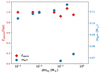 |
Fig. B.2. Values of Eejecta (red diamonds, whose scale is on the left-hand y-axes) and m56Ni (blue points, whose scale is on the right-hand y-axis) as function of dminj. |
Figure B.2 shows the values that we find for Eejecta and m56Ni for different values of dminj. We studied the variation of the outcomes of the explosion assuming dtinj = 10−9s and dEinj = 2.0 foe, and by injecting the thermal energy at the arbitrary mass coordinate of 0.8M⊙. The values we find for Eejecta and m56Ni are also reported in Table D.2.
We find that if we choose to inject the energy in thinner layers, the explosion is more energetic, and because of this when the shock reaches the silicon shell, the explosive Si-burning is more efficient, with respect to scenarios with larger dminj. Thus, in these cases we have an overproduction of 56Ni and the outcome of the explosion do not match the observations of SN1987A.
Our simulations are in agreement with the observations for dminj = 0.1M⊙ and dminj = 0.4M⊙. We chose dminj = 0.1M⊙, since our goal was to obtain a parameter set in good agreement with the observation of SN1987A, not the best parameter set because such analysis would have required a more sophisticated approach, and to calibrate on multiple SN sources. We will explore this aspect in an upcoming work.
B.3. Calibration of dtinj
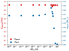 |
Fig. B.3. Values of Eejecta (red diamonds, whose scale is on the left-hand y-axes) and m56Ni (blue points, whose scale is on the right-hand y-axis) as function of dtinj. |
Figure B.3 shows the values that we find for Eejecta and m56Ni for different values of dminj. We studied the variation of the outcomes of the explosion assuming dtinj = 10−9s and dEinj = 2.0 foe, and by injecting the thermal energy at the arbitrary mass coordinate of 0.8M⊙. The values we find for Eejecta and m56Ni are also reported in Table D.3.
we find that the Eejecta is roughly independent on the timescale over which we inject the energy. On the other hand, the amount of 56Ni produced (i.e. the efficiency of the explosive Si-burning) is strongly dependent on dtinj. From Figure B.3 we see that m56Ni is constant for dtinj ≤ 10−3s, while for longer timescales the efficiency of the explosive nucleosynthesis increases, resulting in an overproduction of 56Ni with respect to SN1987A. The value of m56Ni reaches its maximum for dtinj = 0.1s, with  , while on longer timescales it start decreasing. This is because the shockwave reaches the Si shell, where the production of 56Ni takes place, at ∼0.2s. Thus, if the thermal energy is not completely injected before this moment, the shockwave will not have enough energy to trigger the complete explosive Si-burning. This is apparent from Figure B.3 because for dtinj ≥ 0.2s the amount of 56Ni produced is about an order of magnitude lower than what we obtain for lower dtinj. Finally, the values of dtinj that is closer to the observative properties of SN1987A is dtinj = 0.01s, for which we obtain exactly
  , which is the value one usually can find in the literature (e.g., Arnett et al. 1989; Shigeyama & Nomoto 1990; Utrobin 1993, 2006; Blinnikov et al. 2000).
Appendix C: Tables
Results of the interpolation described in Sec. 2.3.
Final properties of stars with various initial metallicities and initial masses for the non-rotating stellar progenitors.
Final properties of stars with various initial metallicities and initial masses for the rotating stellar progenitors.
Appendix D: Calibration tables
Calibration on Einj.
Calibration on dminj.
Calibration on dtinj.
All Tables
Final properties of stars with various initial metallicities and initial masses for the non-rotating stellar progenitors.
Final properties of stars with various initial metallicities and initial masses for the rotating stellar progenitors.
All Figures
|
Fig. 1. Final kinetic energy of the ejecta as a function of the ejected mass of 56Ni obtained running various explosion tests (blue crosses) with different values of the initial explosion parameters, Einj, dminj, and dtinj. The red dot refers to the simulation of the explosion that best matches the properties of SN1987A (orange star). |
| In the text | |
|
Fig. 2. Mass at the pre-SN stage (top-row panels) and CO core mass (bottom-row panels) as a function of MZAMS for the non-rotating progenitors (left panels) and progenitors rotating with an initial velocity of 300 km/s (right panels). Different colors represent different initial metallicities: [Fe/H] = 0 (dashed light blue line), [Fe/H] = −1 (dash-dotted violet line), [Fe/H] = −2 (orange solid line), and [Fe/H] = −3 (dotted yellow line). |
| In the text | |
|
Fig. 3. Chemical composition as a function of the interior mass coordinate of a non-rotating model with MZAMS = 25 M⊙ and [Fe/H] = −2 at the pre-SN stage. We show the chemical composition up to the mass coordinate of 15 M⊙. We report the abundances of H (black line), He (red line), 12C (green line), 16O (blue line), 20Ne (magenta line), 28Si (orange line), 52Cr (dark red line) and 56Fe (gray line). |
| In the text | |
|
Fig. 4. Temperature profile (solid red line) and mass density profile (dash-dotted black line) of the stellar progenitor at the pre-SN stage as a function of the mass coordinate. A zoom-in on the innermost region of the core, up to 5 M⊙, is highlighted in the lower-left box. |
| In the text | |
|
Fig. 5. Velocity of the shock wave as a function of the mass coordinate at different times after the onset of the explosion. The end of the explosive nucleosynthesis (dotted blue line), the shock wave enters the CO core (dash-dotted orange line), the shock wave reaches the He/H interface (solid green line), 1000 s after the onset of the explosion (dashed red line), the formation of the compact remnant (long dashed purple line), and the shock breakout (short dot-dashed light green line). The shaded purple area represents the extension of the final compact remnant. |
| In the text | |
|
Fig. 6. Interior profiles of the kinetic energy (yellow line), the internal energy plus the gravitational energy (purple line), and the total energy (dashed light blue line) at various times during the explosion for a non-rotating stellar progenitor with MZAMS = 25 M⊙ with metallicity [Fe/H] = −2. The shaded purple area in the panels represents the region of the star forming the compact remnant at each time. It is completely formed at t = 3 × 10⁴ s. |
| In the text | |
|
Fig. 7. Evolution of the radius of various shells (gray and dotted purple lines) inside the stellar progenitor as a function of time. Each gray (dotted purple) line on top encloses 1 M⊙ (3 M⊙) more than the gray (dotted purple) line immediately below. We also show the evolution of the radius of the final compact remnant (yellow dashed line). |
| In the text | |
|
Fig. 8. Chemical composition as a function of the interior mass coordinate of a non-rotating model with MZAMS = 80 M⊙ and [Fe/H] = −2 at the pre-SN stage. We report the abundances of H (long dash-double dotted black line), He (double dash-dotted red line), 12C (long dashed green line), 16O (short dashed blue line), 20Ne (dashed magenta line), 28Si (short dash-double dotted orange line), 52Cr (solid dark red line) and 56Fe (long dash-dotted gray line). |
| In the text | |
|
Fig. 9. Temperature profile (red line) and density profile (dash-dotted black line) at the pre-SN stage as a function of the mass coordinate of a non-rotating stellar progenitor with MZAMS = 80 M⊙ and [Fe/H] = −2. A zoom-in on the innermost region of the core, up to 5 M⊙, is highlighted in the lower right box. |
| In the text | |
|
Fig. 10. Same as Figure 5 but for a directly collapsing progenitor. The velocity profile is reported at different crucial times during the explosion: when the explosive nucleosynthesis stops (dotted blue line), when the layers behind the shock start to fallback onto the compact remnant (dash-dotted orange line), when the shock enters the CO core (dashed green line) and when the velocity of the shock becomes negligible (solid red line). |
| In the text | |
|
Fig. 11. Same as Figure 7 but for the most central region of the progenitor with MZAMS = 80 M⊙ and [Fe/H] = −2, where we can better appreciate the fallback of the layers right after being accelerated by the shock wave. We show the behavior of the shell enclosing different values of mass, of 1 M⊙ (each solid light gray lines) and 5 M⊙ (each dotted purple line), respectively. |
| In the text | |
|
Fig. 12. Remnant masses as a function of MZAMS for the progenitors with initial metallicity [Fe/H] = 0 (dashed light blue line), [Fe/H] = −1 (dash-dotted violet line), [Fe/H] = −2 (orange solid line), and [Fe/H] = −3 (dotted yellow line). We do not simulate the explosion of the stellar progenitors with MZAMS = 120 M⊙ at subsolar metallicities, since they are unstable against pair production. |
| In the text | |
|
Fig. 13. Pre-SN mass (dash-dotted light blue line), pre-SN mass extrapolated for MZAMS > 120M⊙ (dotted gray line), remnant mass (solid violet line), and the remnant mass for the stars that develop pair instabilities (dashed yellow line), as a function of MZAMS. The red points represent the stellar progenitors of the FRANEC grid, while the larger red squares correspond to the last progenitor stable against pair production, which has been obtained through interpolation (see Sect. 2.3 and Table C.1). The shaded gray area represents the region of DC, the shaded yellow area shows where stars undergo PPISNe. The vertical dashed lines represent the threshold values above which stars enter the PI regions. |
| In the text | |
|
Fig. 14. Same of Figure 12 but for rotating progenitors. We do not simulate the explosion of the stellar progenitors with MZAMS = 80 M⊙ and 120 M⊙ at [Fe/H] = −2, −3, since they are unstable against pair production. |
| In the text | |
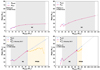 |
Fig. 15. Same as Figure 13 but for rotating progenitors. |
| In the text | |
|
Fig. 16. Maximum BH mass as a function of the initial metallicity for the non-rotating stellar progenitors (red line) and the rotating stellar progenitors (blue line) for the non-rotating progenitors. |
| In the text | |
|
Fig. 17. Black hole mass spectrum as a function of the CO core mass from various authors. Solid blue line: this work, non-rotating progenitors at [Fe/H] =−3; long dashed orange line: set D of W17 (we note that these models are obtained from stellar tracks computed at Z = 0.1 Z⊙ for which the mass loss has been inhibited, making these models distinct from those we used to compute the final remnant masses.); dashed pink line: models from Spera & Mapelli (2017) with Z = 1.3 × 10⁻² Z⊙ (S17). Circles (crosses) represent the models that are stable (unstable) against pair production, and squares are the stars disrupted by PISNe. |
| In the text | |
|
Fig. 18. Black hole mass spectrum as a function of the CO core mass for different PPISN prescriptions. Solid blue line: this work, non-rotating progenitors at [Fe/H] =−3; dash-dotted orange line: F19 PPISN threshold ( |
| In the text | |
|
Fig. 19. Normalized probability distribution of BH masses we obtained from a population of 106 stars whose mass follows a Kroupa (2001) mass function (i.e., |
| In the text | |
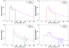 |
Fig. 20. Same as Figure 19 but for rotating progenitors. |
| In the text | |
|
Fig. 21. Linear relation between the mass that falls back after the explosions and some structural properties of the stellar progenitors at the pre-SN stage, such as the absolute value of the total energy (top panels), the binding energy (central panels), and the CO core mass (bottom panels). We have performed such analysis both for the non-rotating (left panels) and for the rotating stellar progenitors (right panels). We studied the fate of the explosion independently of the initial metallicity. Thus, in each panel we have all the models with [Fe/H] = 0 −1, −2, −3. In each panel the circular orange points are the stellar progenitors undergoing successful SN explosions and the best fit for dM/M is the solid red line, while the diamond purple points represents the progenitors which DC to BHs. The black dashed line corresponds to dM/M = 1 i.e., the value of dM/M for the DC. The red shaded area is the 95% confidence interval for the SN linear regression. |
| In the text | |
|
Fig. B.1. Values of Eejecta (red diamonds, whose scale is on the left-hand y-axes) and m56Ni (blue points, whose scale is on the right-hand y-axis) as function of Einj. |
| In the text | |
|
Fig. B.2. Values of Eejecta (red diamonds, whose scale is on the left-hand y-axes) and m56Ni (blue points, whose scale is on the right-hand y-axis) as function of dminj. |
| In the text | |
|
Fig. B.3. Values of Eejecta (red diamonds, whose scale is on the left-hand y-axes) and m56Ni (blue points, whose scale is on the right-hand y-axis) as function of dtinj. |
| In the text | |
Current usage metrics show cumulative count of Article Views (full-text article views including HTML views, PDF and ePub downloads, according to the available data) and Abstracts Views on Vision4Press platform.
Data correspond to usage on the plateform after 2015. The current usage metrics is available 48-96 hours after online publication and is updated daily on week days.
Initial download of the metrics may take a while.