| Issue |
A&A
Volume 695, March 2025
|
|
|---|---|---|
| Article Number | A58 | |
| Number of page(s) | 13 | |
| Section | The Sun and the Heliosphere | |
| DOI | https://doi.org/10.1051/0004-6361/202451479 | |
| Published online | 07 March 2025 | |
Comparative analysis of two episodes of strongly geoeffective coronal mass ejection events in November and December 2023
1
Institute of Physics, University of Graz, A-8010 Graz, Austria
2
Hvar Observatory, Faculty of Geodesy, University of Zagreb, Zagreb, Croatia
3
Department of Physics and Astronomy, Queen Mary University of London, Mile End Road, London E1 4NS, UK
4
INAF – Osservatorio Astrofisico di Torino, Via Osservatorio 20, 10025 Pino Torinese (TO), Italy
5
Dip. di Fisica e Astronomia, Università di Firenze, Via Sansone 1, 50019 Sesto Fiorentino (FI), Italy
⋆ Corresponding author; This email address is being protected from spambots. You need JavaScript enabled to view it.
Received:
12
July
2024
Accepted:
21
January
2025
Abstract
Context. In autumn 2023 a series of close-in-time eruptive events were observed remotely and measured in situ. For that period, we studied a set of analogous events on the Sun, where several coronal mass ejections (CMEs) were launched partly from the same (active) regions close to a coronal hole. The two episodes of events are separated by a full solar rotation covering the period October 31–November 3 and November 27–28, 2023.
Aims. The two episodes of eruptive events are related to strong geomagnetic storms occurring on November 4–5 and December 1–2, 2023. We point out the complexity for each set of events; our aim is to understand how the global magnetic field configuration, solar wind conditions, and interaction between the structures relate to these geomagnetic effects.
Methods. We used the graduated cylindrical shell (GCS) 3D reconstruction method to derive the direction of motion and speed of each CME. The GCS results served as input for the drag-based model with enhanced latitudinal information (3D DBM), facilitating the assessment of its connection to in situ measurements. This approach significantly aids in the integrated interpretation of in situ signatures and solar surface structures.
Results. The first episode caused visible stable auroral red (SAR) arcs, with a Dst index that dropped in three steps down to −163 nT on November 5, 2023. Close in time, two CME-related shocks arrived, separated by a sector boundary crossing (SBC), and followed by a short-duration flux rope-like structure. For the second episode, auroral lights were observed related to a two-step drop in the Dst index down to −108 nT on December 1, 2023. A shock from a CME within the magnetic structure of another CME ahead was identified, again combined with a SBC. Additionally, a clear flux rope structure from the shock producing CME was detected. In both events, we observed distinct short-term variations in the magnetic field (“ripples”) together with fluctuations in density and temperature that followed the SBC.
Conclusions. The study presents a comparative analysis of two episodes of multiple eruptive events in November and December 2023. In addition to the interacting CME structures, we highlight modulation effects in the geomagnetic impact due to magnetic structures that are related to the SBC. These most likely contributed to the stronger geomagnetic impact and production of SAR arcs for the November 4–5, 2023, event. At the Sun, we found the orientation of the heliospheric current sheet to be highly tilted, which might have caused additional effects, due to the CMEs interacting with it.
Key words: Sun: activity / Sun: coronal mass ejections (CMEs) / Sun: heliosphere / solar-terrestrial relations / solar wind
© The Authors 2025
 Open Access article, published by EDP Sciences, under the terms of the Creative Commons Attribution License (https://creativecommons.org/licenses/by/4.0), which permits unrestricted use, distribution, and reproduction in any medium, provided the original work is properly cited.
This article is published in open access under the Subscribe to Open model. This email address is being protected from spambots. You need JavaScript enabled to view it. to support open access publication.
1. Introduction
Based on results from cycle 23, the rates of intense geomagnetic storms during maximum and declining solar cycle phases are found to be almost three and two times as high as during the rising phase of a solar cycle (Echer et al. 2008). This is mainly due to numerous eruptive flares occurring close in time and space, resulting in multiple coronal mass ejections (CMEs) that jointly evolve and may interact in interplanetary space (see reviews by, e.g., Lugaz et al. 2017; Manchester et al. 2017; Zhang et al. 2021). An increased number of solar eruptions create extraordinary conditions in near-Earth space, commonly known as space weather (see, e.g., Cliver & Svalgaard 2004; Bothmer et al. 2007). Severe impacts on near-Earth space are usually related to the enhanced strength and complexity of the magnetic field in the impacting solar events (see, e.g., the “panoramic” paper by Tsurutani et al. 2023, presenting in a combined overview our gained knowledge of space physics and space weather over the past 65 years).
The complexity of the interplanetary magnetic field sweeping over Earth typically increases due to the interaction between multiple large-scale magnetic structures. These interactions cover not only CMEs, but also co-rotating interaction regions (CIRs) formed by high-speed solar wind streams originating from coronal holes (CHs) or the heliospheric current sheet (HCS). It is broadly accepted that all these components evolving together as compound interplanetary magnetic structures cause much stronger geomagnetic effects compared to their isolated appearance (e.g., Echer & Gonzalez 2004; Dumbović et al. 2015). It should be noted that the occurrence of successive CMEs or merged interaction regions do not always cause stronger geomagnetic effects, especially when related to northward Bz components (see Burlaga & Plunkett 2002; Burlaga et al. 2003). Propagating shocks caused by energetic CMEs, when penetrating through a CME ahead are prone to enhancing the magnetic field complexity (Lugaz et al. 2016). In-depth case studies investigate the process of CME-CME interaction (e.g., Gopalswamy et al. 2001; Temmer et al. 2012; Scolini et al. 2020), or CME-CIR interaction (e.g., Fenrich & Luhmann 1998; Heinemann et al. 2019a; Winslow et al. 2021; Geyer et al. 2023). However, the details of the interaction processes between these different structures are still not well understood. This complicates the interpretation of in situ measurements and the development of reliable models for forecasting geomagnetic effects.
Compared to 20 years ago, during the peak of solar cycle 23, the coverage (multiple viewpoints, varying distances including heliospheric imagers) and quality (temporal and spatial resolution) of solar data have improved substantially. These advancements have been accompanied by significant progress in our investigation techniques and modeling approaches. Solar cycle 24 was notably weak (e.g., McComas et al. 2013), which made it challenging to test our understanding of complex solar activity phenomena. The current solar cycle, cycle 25, appears to be more similar to cycle 23 in terms of geomagnetic effects and the complexity of the related phenomena (see, e.g., Berdichevsky et al. 2000; Burlaga & Plunkett 2002; Burlaga et al. 2003). Events occurring at the end of October and beginning of November 2023 produced intricate in situ measured profiles together with strong auroral light activities. In addition to auroral lights, a special type of atmospheric light phenomena, called stable auroral red (SAR) arcs (Cole 1965), were observed almost globally on November 5, 2023, reaching even southern Europe. SAR arcs are known to be related to extreme conditions in Earth’s ring current system (see review by, e.g., Kozyra & Liemohn 2003). In addition to SAR arcs, on November 5, 2023, a very rarely observed anisotropic cosmic-ray enhancement (ACRE) was also reported by Gil et al. (2024). A full rotation later, at the end of November 2023, a series of CMEs again launched and were heading toward Earth. These events resulted in strong geomagnetic effects, but to a comparatively weak disturbance storm time (Dst) index (−108 nT for December 1, 2023, vs. −163 nT for November 5, 2023) and no SAR arcs.
For the present study we investigated these two episodes of CME events to understand their similarities as well as differences. The two episodes are united by the involvement of similar active regions and the same CH, but are separated in time by a complete solar rotation. We performed a thorough investigation of the solar source regions, CME development, and potential interaction with the nearby high-speed stream emanating from the CH. This was complemented by modeling efforts to better match and interpret in situ measurements, focusing on the arrival time and impact of each event. To model the interplanetary propagation behavior of the CMEs, we applied the drag-based-model (DBM; Vršnak et al. 2013) in an enhanced 3D version (3D DBM; Dumbovic et al., in prep.), which covers latitudinal information. We highlighted the importance of HCS orientation and crossings, which enhance the complexity of solar activity phenomena and their impact on planets (see also COSPAR Space Weather Roadmap update by Temmer et al. 2023).
The paper is structured as follows. In Sect. 2 we investigate the solar perspective and use the results to run the 3D DBM propagation model. With this we assess the impact likeliness and arrival time of each CME at Earth to better link and interpret the in situ signatures. In Sect. 3 we analyze the in situ measurements for each rotation and relate them to the geomagnetic impact. In Sect. 4 we present a discussion and our conclusions. Appendices A and B cover the complementary material for the analysis and methodology, respectively.
2. The solar perspective
2.1. Data and methods
We investigated two episodes of multiple eruptions from the Sun covering the time range October 31–November 3, 2023 (rotation #1), within Carrington rotation 2277, and November 27–28, 2023 (rotation #2), within Carrington rotation 2278. Separated by a full solar rotation, the two episodes of events show many similarities, as partly the same (active) regions are involved, which are located primarily to the west of the same CH (see Fig. 1 for more details, and Sects. 2.2 and 2.3).
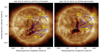 |
Fig. 1. General overview of the CME occurrence and CHs for the two episodes, rotation #1 (left panel) and rotation #2 (right panel), overlaid on AIA 193 Å images. Given are the CH locations with their center of mass (CM) and apex distances to the active regions (AR) from which the CMEs were launched (see details in Sect. 2.1). For each CME the 3D speed information is given as derived from a linear fit to sequential GCS reconstructions. For rotation #1 we observe four CMEs (CME1.1–1.4) and for rotation #2 five CMEs (CME2.1–2.4+5). We note that for CME 2.1 the corresponding active region is already behind the western limb, and therefore no AR distance is given. The image dates were chosen such that the CH is centrally located for better visibility. |
To study the solar surface structures of the erupting events, the related filaments and flares, as well as their magnetic properties, we used data from the Solar Dynamics Observatory (SDO; Pesnell et al. 2012). These cover extreme ultraviolet (EUV) images from the Atmospheric Imaging Assembly (AIA; Lemen et al. 2012) together with photospheric magnetic field information from the Helioseismic and Magnetic Imager (Scherrer et al. 2012). Figure 1 provides an overview of the eruption sites of the CMEs relative to the CH for rotation #1 and #2, superimposed on an AIA 193Å image. For each evolving CME we apply the graduated cylindrical shell (GCS) model on stereoscopic white-light coronagraph data (Thernisien et al. 2006). GCS simulates the flux rope structure that is often associated with CMEs. Fitting the model to coronagraph images from at least two different viewpoints enables us to obtain the 3D CME geometry and propagation direction. Applying that procedure over several time steps allows us to derive the 3D speed. Error estimates for the height-time measurements from the GCS reconstructions and derived speeds are on the order of 5%, as given by Verbeke et al. (2023). We used the time series of white-light data from the Large Angle Spectroscopic Coronagraph aboard the Solar and Heliospheric Observatory (SOHO/LASCO C2 and C3; Brueckner et al. 1995) and the COR2 coronagraph from the Sun Earth Connection Coronal and Heliospheric Investigation (SECCHI; Howard et al. 2008) aboard the Solar Terrestrial Relation Observatory (STEREO-A; Kaiser et al. 2008). During that period we had only a small separation between STEREO-A and SOHO (5–7°). To better constrain the GCS forward model, we added Metis coronagraph data (visible light VD channel at 610 nm; Antonucci et al. 2020; Fineschi et al. 2020; De Leo et al. 2023) from Solar Orbiter (Müller et al. 2020). Solar Orbiter is located east of the Earth with a separation of ∼20° for rotation #1 events and ∼10° for rotation #2 events.
Coronal holes are the main sources of fast solar wind emanating along the open magnetic field within the CH and interacting with the slow solar wind ahead, forming CIRs (see, e.g., review by Cranmer et al. 2017). The CH under study, which is the same for all the events, is investigated using CATCH (Heinemann et al. 2019b). Results from CATCH and GCS are used to calculate the coronal hole influence parameter (CHIP). The CHIP assesses the influence of the CH on each CME and is calculated from the line-of-sight magnetic field strength and area of the CH in relation to the CME’s source region distance (see Gopalswamy et al. 2009, and references therein). The CHIP value (in gauss) is given for the distance between the CH center of mass and the projection of the CME apex on the solar disc. The derived distances (labeled “AR_apex”) are given in Fig. 1. The CHIP reveals the impact of the CH on the behavior of CME propagation, particularly its potential to divert the CME magnetic structure from its radial trajectory.
Utilizing the results from the GCS reconstruction, we were able to generate a projected view of each CME using a straightforward cone geometry, considering both equatorial and meridional planes (equations outlined in Dumbovic et al., in prep.). The CME cone projections enabled us to more easily (or better) connect remote sensing imagery with in situ data. This allowed us to determine which CME, and more specifically which region of the CME (apex, flank), is most likely associated with the in situ measurements. Covering the GCS error estimates, we calculated the best- and worst-case impact scenarios representing conditions that are either more favorable for a hit or more likely to result in a miss.
Table 1 gives a summary for each CME and its source region characteristics (block 1), CATCH and CHIP results for the CH (block 2), and 3D DBM hit and miss statistics (block 3). A summary of all the derived GCS parameters, their errors, and hit-miss likeliness is given in Table A.1.
Summary table.
2.2. Near-Sun results for rotation #1
During the first rotation we focused on the occurrence of four prominent CMEs, termed CME1.1, 1.2, 1.3, and 1.4. For rotation #1, the top left panels of Fig. 2 provide an overview of the eruption sites. The bottom left panels show the projected cone geometries for each CME as derived from the GCS results. In addition to LASCO C2 and COR2 data, Metis observations were available for CME1.1, CME1.2, and CME1.4. We present in Fig. 3 the GCS reconstruction and kinematics on the example of CME1.2. All other GCS reconstruction plots from rotation #1, together with the height-time plots, linear fits, and speed derivations, are given in Figs. A.1–A.3.
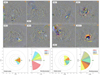 |
Fig. 2. Overview of the eruption sites and CME cone projections. Top panels: SDO/AIA EUV composite ratio images (source: suntoday.lmsal.com) for each eruptive event. Bottom panels: CME cone geometry derived from GCS results (longitude, latitude, tilt) projected on the ecliptic and meridional plane. The events are annotated with the eruption related GOES SXR flare classes. Left panels: Rotation #1 over the period from 2023-10-31 21:27 UT to 2023-11-03 05:52 UT. CME1.1+1.2+1.4 are related to filament eruptions f1+f2+f3, respectively. Right panels: rotation #2 over the period 2023-11-27 18:48 UT until 2023-11-28 19:50 UT. CME2.1+2.4 are related to filament eruptions f1+f2, respectively. |
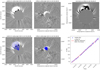 |
Fig. 3. For rotation #1 we show on the example of CME1.2 the CME structure from different perspectives (LASCO C2, COR2, and Metis) and GCS reconstruction for the CME at a 3D height of 5.4Rs. Bottom right panel: from different time steps the height-time and speed are derived using a linear fit (given in the legend). |
CME1.1 started from a filament eruption at around 2023-10-31 20:00 UT, located in the southern hemisphere spanning heliographic coordinates S18–S40/E00–E40. The eruption site is not related to an active region. The CME was observed in white-light image data with a first appearance in LASCO C2 at 2023-10-31 22:12 UT at the position angle (PA) 160–200°. Tracking the CME over time and performing GCS reconstruction for each time stamp, we derived a speed of ∼650 ± 30 km/s. From the orientation of magnetic tongues, filament barbs, and post-eruptive arcades (PEAs) it could be related to a right-handed chirality (see, e.g., Palmerio et al. 2018). The projected view of the CME in simple cone geometry in the meridional cut reveals that the CME primarily moves to the south. From the best-hit scenario, CME1.1 would only be a glancing blow.
CME1.2 is related to a filament eruption at 2023-11-02 ca. 03:00 UT, located in the northern hemisphere at the heliographic coordinates N25/E25. The eruption site is not related to an active region. The CME was observed in white-light image data with a first appearance in LASCO C2 at 2023-11-02 03:36 UT at PA 0–70°. From GCS reconstructions we calculated a speed of ∼630 ± 30 km/s. The chirality was derived as left-handed. The projected cone geometry from GCS shows that the CME moves far away from the Sun-Earth line directed to the northeast. In the best-hit scenario, CME1.2 would miss Earth.
CME1.3 is not related to a filament eruption, but to an active region (AR 13474) that produced two flares with a time difference of about 8 hours: an M1.7 (GOES SXR-class) flare peaking at 2023-11-02 12:22 UT and a C2.8 flare with its maximum at 20:18 UT. The flare location is given at the heliographic coordinates S18/W30-34. In LASCO C2 the CME front appeared first at 2023-11-02 23:12 UT at PA 260–280°. Though the CME itself is weak, with a speed of ∼350 ± 20 km/s as derived from GCS reconstruction, it seems to have destabilized the filament related to CME1.4 erupting the following day. The chirality for this complex two-flare source region could not be unambiguously derived, as no magnetic tongues, sigmoids, post-eruptive flare ribbons, or filament barbs could be identified. The projected cone geometry from GCS shows that the CME propagates in the western direction, away from the Sun-Earth line. In the best-hit scenario, CME1.3 would be a flank hit.
CME1.4 was produced due to a large filament eruption starting to rise at 2023-11-03 06:00 UT in the northwestern hemisphere spanning a heliographic range of N00-N30/W00-W60. The source region is related to AR 13473. The filament rise is preceded by a C3.2 flare starting at 2023-11-03 04:40 UT at N31W26. The first LASCO C2 image shows the CME front at 2023-11-03 05:48 UT, and that it continues to evolve as partial halo event. From GCS reconstructions we derived a speed of ∼1190 ± 60 km/s. The chirality for the flux rope was derived as left-handed. From the projected GCS cone we see that the CME flux rope part propagates slightly northward from Earth. Applying nominal GCS parameters and those producing a best-hit, CME1.4 would result in a glancing blow or even a full hit for Earth.
The CH polarity was derived to be negative (signed/unsigned mean magnetic field strength of −5.2 G/12.2 G). The size in area of the CH (8.5 × 10¹⁰ km2) would be related to a high-speed stream with a speed at 1AU on the order of ∼750 km/s (see Vršnak et al. 2007). Using these results, the calculated CHIP parameter for each CME reveals values well below 2.6 G, which was found as a lower limit corresponding to the deflecting effect by a CH (Mäkelä et al. 2013).
To summarize, the speeds for CMEs 1.1–1.3 are found to be in the slow to moderate range with values at 21.5 Rs on the order of 350–650 km/s. CME1.4 is the most energetic event, revealing ∼1190 km/s at 21.5 Rs, and is related to a huge filament eruption. Due to the low CHIP values found, we do not expect any of the CMEs to be significantly deflected from their directions as derived from low coronal signatures. Interpreting the source surface information, 3D geometries of the CMEs, and reconstructed speeds, we conclude that only CME1.4 is a potential candidate to partially hit Earth, with CME1.3 as the most likely additional candidate. Because it is a miss even in the best-hit scenario, we confidently exclude CME1.2 as a candidate for appearing in the in situ signatures and we would categorize CME1.1 as unlikely to cause significant in situ signatures.
2.3. Near-Sun results for rotation #2
During the second rotation, we focused on the occurrence of five CMEs. For rotation #2, the top right panels of Fig. 2 provide an overview of the eruption sites. The bottom right panels show the projected cone geometries for each CME as derived from the GCS results. In addition to LASCO C2 and COR2 data, Metis observations were available for CME2.1, CME2.3, and CME2.4+5. We present in Fig. 4 the GCS reconstruction and kinematics on the example of CME2.3. The GCS reconstruction plots for all other CMEs from rotation #2, together with the height-time plots and linear fits, as well as speed derivation, are given in Figs. A.4–A.6.
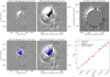 |
Fig. 4. For rotation #2 we show on the example of CME2.3 the CME structure from different perspectives (LASCO C2, COR2, and Metis) and GCS reconstruction for the CME at a 3D height of 13.0 Rs. Bottom right panel: from different time steps the height-time and speed are derived using a linear fit (given in the legend). |
CME2.1 is related to a filament eruption (close to AR 13499) starting at 2023-11-27 ca. 05:00 UT from heliographic coordinates around W30/S30. It appears in LASCO C2 images at 2023-11-27 06:48 UT at PA 150–250°. Performing GCS reconstructions we derived a speed of ∼550 ± 30 km/s. The chirality was derived from the orientation of the PEA and underlying magnetic field as right-handed. The projected cone geometry from GCS shows that the CME moves far away from the Sun-Earth line directed to the south, but might affect subsequent CMEs due to its large width in longitude. From the best-hit scenario, CME2.1 would be a flank hit.
CME2.2 is related to a C6.7 flare starting 2023-11-27 18:52 UT at N18E09 (east from AR 13503) with further activity signatures connecting to the south (AR 13500), presumably via some global magnetic field that might have been disturbed as CME2.2 erupted. It appears in the LASCO coronagraphs as a partial halo revealing its front in the C2 field of view for the first time at 2023-11-27 20:12 UT. Tracking the CME over time and performing GCS reconstructions, we derived a speed of ∼520 ± 30 km/s. The chirality was derived as left-handed. The projected cone geometry from GCS would suggest a direct impact on Earth, with the hit occurring relatively close to the CME apex. From the best-hit scenario, CME2.2 would be a full apex hit.
CME2.3 is related to a filament eruption and C5.6 flare at 2023-11-27 23:40 UT located at N26E40. The source region is located west from AR 13503. In LASCO C2 it first appears at 2023-11-27 23:48 UT at PA 0–90°. From GCS reconstructions we derived a speed of ∼1020 ± 50 km/s. The chirality was derived as left-handed. The projected cone geometry from GCS shows that the CME moves far away from the Sun-Earth line directed to the northeast. For the best-hit scenario, CME2.3 would miss Earth.
CME2.4+5 is related to an extended double eruptive event on 2023-11-28 with two strong flares (M3.4+M9.8) from a source region located at heliographic coordinates S16W00 (AR 13500). The observed signatures of a coronal wave indicate a strong lateral expansion of the CME (see, e.g., review by Patsourakos & Vourlidas 2012). The M3.4 flare from 2023-11-28 peaked at 19:32 UT immediately followed by a M9.8 flare with a maximum at 19:50 UT. The CME is reported in LASCO as a full halo and the double-eruption shows fronts close in time at 2023-11-28 20:24 UT and 20:48 UT. From the short time difference we can safely presume that the CMEs started to interact close to the Sun, and therefore they will be treated as a single eruption. Tracking the outermost CME front we derived from GCS reconstructions a speed of ∼640 ± 30 km/s. The chirality for the eruptions from that source region was derived as right-handed. The projected cone geometry from GCS reveals a hit due to its huge extent. Even for the worst-hit scenario, CME2.4+5 would still be classified as a hit.
The CH polarity was found to have decreased in its magnetic field strength (signed/unsigned mean magnetic field strength of −3.5 G/10.9 G). On the other hand, the area was found to have increased to 10.1 × 10¹⁰ km2. This non-correlation between area and magnetic field strength supports findings by Heinemann et al. (2020) who concluded that the magnetic flux within a CH is not the main cause for its evolution. Again we derived for each of the CME events very low CHIP values, indicating little or no influence of the CH on any of the CME trajectories.
In summary, CME 2.1, 2.2, and 2.4+5 (double eruptive event) show rather moderate speeds with 520–640 km/s at the height of 21.5 Rs, while CME2.3 is derived with ∼1020 km/s. Interpreting the source surface information, 3D geometries of the CMEs, and reconstructed speeds, we conclude that CME2.2 and CME2.4+5 would most likely hit Earth. Since CME2.3 is a miss even under the best-hit scenario, we confidently rule it out as a candidate for being detected as in situ signature. CME2.1 is identified as unlikely to cause in situ signatures.
3. Interplanetary space perspective
3.1. Data and methods
The in situ measurements are from the OMNI_HRO_1MIN dataset, which was provided by the Coordinated Data Analysis Web1. The data cover 1 minute resolution time series of solar wind plasma parameters and interplanetary magnetic field components in the geocentric solar ecliptic (GSE) coordinate system, shifted to the nose of the Earth’s bow shock (King & Papitashvili 2020). From the plasma and magnetic field components we calculated the plasma-β value.
To study and assess the geo-effectiveness, we used the Dst and the half-hourly or hourly, planetary open-ended (Hpo) indices. The Dst index measures the average deviation in the horizontal component of the Earth’s magnetic field as well as the plasma energy content of the inner magnetosphere at mid-latitude stations around the globe (see, e.g., Turner et al. 2001). For the analysis we used the provisional Dst index2 with a 1 hour time resolution. The geomagnetic Hpo index describes, in a similar way to the Kp (planetarische Kennzahl) index, the disturbance levels in the two horizontal magnetic field components. In comparison to Kp with 3 hour time resolution scaling from 0 to 9, the Hpo index is derived with a higher time resolution of 30 and 60 minutes, respectively, and its scale is open-ended. For our studies we used Hp303 covering a temporal resolution of 30 minutes (Yamazaki et al. 2022).
To establish the connection between results derived from remote sensing image data and in situ measurements, we utilized the analytical drag-based model (DBM). Simulations were conducted for CME1.4, CME2.2, and CME2.4+5, which were identified as potential candidates for exhibiting in situ signatures. The results from the GCS model (3D geometry, speed, and direction of motion) were used as input parameters to derive the arrival time and speed of the flux rope (i.e., magnetic structure) of the CME (Vršnak et al. 2013). DBM was recently modified for 3D CME geometry (3D DBM; Dumbovic et al., in prep.). DBM usually uses GCS results to calculate the extent of the CME in the solar equatorial plane and runs the CME leading edge as a non-self-similarly expanding 2D cone (Dumbović et al. 2021a). 3D DBM takes into account the heliographic latitude or the extent of the CME in the solar meridional plane, applying the geometry of the non-self-similarly expanding 2D cone in both the solar equatorial and the meridional plane (cf. bottom panels of Fig. 2). Moreover, 3D DBM can be used to model the CME-CME interaction in a very simple manner (shown by, e.g., Guo et al. 2018; Dumbović et al. 2019, using DBM) as outlined in Appendix B. We acknowledge that this is a simplified approach; however, it serves the purpose of linking CMEs to their in situ measurements. For a more comprehensive and physically detailed analysis of CME-CME interactions, we refer to the advanced MHD models by Lugaz et al. (2005) or Scolini et al. (2020).
Table 1 gives a summary of the 3D DBM results for shock and flux rope arrival time (block 3) as well as in situ measured times for comparison (block 4). The related GCS input parameters to run the 3D DBM are given in Table A.1.
3.2. In situ results for rotation #1
The results from the projected cone geometries show that CME1.1 and 1.2 miss Earth and CME1.3 most likely misses Earth. Only CME1.4 is derived to partly hit Earth. Based on these results, we would therefore not expect clear signatures of a magnetic ejecta (ME) in the in situ measurements from any of the CMEs. For CME1.4 we calculated with 3D DBM the arrival time with November 5, 2023, at 23:00 UT, with a tentative shock-sheath arrival 10 hours earlier (i.e., 13:00 UT). We note that this tentative shock arrival time is estimated based on the typical shock–sheath duration from a statistical approach, as given by Russell & Mulligan (2002).
The left panel of Fig. 5 shows an overview of Earth-related measurements for rotation #1. In situ measurements reveal two shocks very close in time at November 5, 2023, at 09:09 UT and 12:38 UT. Between these two shocks a sector boundary crossing (SBC) is identified; a list of SBCs is maintained by Leif Svalgaard4. SBCs mark the polarity transition across the wavy HCS, which is embedded in a much larger plasma sheet structure (Winterhalter et al. 1994). The HCS signatures (plasma density, total magnetic field) associated with the SBC are not fully clear and could also be interpreted as deflection patterns in the interplanetary magnetic field caused by the CME shocks, likely corresponding to the flank crossings of CME1.3 and CME1.4. The second shock is followed by a prominent short-duration magnetic field structure (12:38–15:09 UT) of low plasma-β (see Fig. A.7 for a zoomed-in version of Fig. 5). Afterward we observe some distinct magnetic field variations that we refer to as ripples (see below for details). November 4, 2023, a day before the first shock-arrival, a high plasma-β region is measured. That high plasma-β structure is followed by a huge increase in density up to ∼60 Np per cm3 and a negative Bz component of about −18 nT. The region hints toward the extended heliospheric plasma sheet (HPS; streamer belt plasma) surrounding the current sheet (Burlaga et al. 1990; Winterhalter et al. 1994). Though the HPS is typically not related to a strong out-of-the-ecliptic field, the closeness to the CME shock might have compressed the HPS. A similar scenario was observed and modeled by Wu et al. (2017). That specific solar wind structure is related to the first drop in Dst to −54 nT at November 4, 2023, around 24:00 UT.
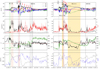 |
Fig. 5. OMNI in situ measurements and geomagnetic indices for each rotation (x-axis shows time in UT). From top to bottom: magnetic field and vector components, density+temperature, plasma-β+speed, Dst+Hp30. Shown are a high plasma-β structure heliospheric plasma sheet (HB), high-density (HD) structures, the shocks (SH; dashed vertical lines) from various CMEs, the sector boundary crossing (SBC; dotted red vertical line), magnetic ejecta (ME) related to the different CMEs, and the start of the SIR/HSS (gray shaded area marks the interaction zone between the rear-part of the CME and the starting of the SIR). The red arrows indicate the observed ripples (short-term variations in the total magnetic field associated with strong fluctuations in the temperature and density profiles). A zoomed-in image for the regions around the SBC is shown in Fig. A.7. |
The arrival of the two CME-related shocks (most likely related to CME1.3 and CME1.4, respectively) cause a slight increase in Dst again, each followed by a second and third drop to −83 nT (November 5, 2023, at 11:00 UT) and −163 nT (November 5, 2023, at 19:00 UT). The second drop in Dst is related to strong fluctuations between the shock-sheath part of CME1.3 and SBC region with a minimum Bz of −24 nT. The third strong Dst drop starts with the arrival of the short-duration magnetic field structure having a minimum Bz of −28 nT and continues to drop further during the ripples. Compared to that, the Hp30 index reached a peak value of 5.33 on November 5, 2023, at 20:00 UT and further increased to 7.00 at 14:30 UT, with peak values of 7.33 between 16:30 and 17:30 UT (low-latitude SAR arcs were reported around 17:30 UT). To conclude, we can attribute the three-step drop in Dst to the occurrence of a high-density and rather strong negative Bz streamer belt plasma related to the HPS, shock-sheath magnetic field fluctuations and specific magnetic field configurations influenced by the sector boundary. A three-step decrease in the Dst is also reported for the complex events in September 2017 by Hajra et al. (2020).
As expected the SIR arrives later on November 6, 2023, at 09:30 UT (marked by a gray area in Fig. 5) with a change in the azimuthal flow angle (not shown), followed by the HSS around 16:30 UT. Interestingly, most of the observed ripples are located in the region before the SIR/HSS and after the shock arrival from CME1.4 that follows the SBC. These kinds of structured signatures reveal short-term variations in the mesoscale range of a few hours in the total magnetic field with either correlated or anti-correlated profiles among the vector components. The small-scale variations are separated by abrupt changes in the magnetic field orientation. The structures are related to strong fluctuations in the temperature and density profiles. We marked the ripples with red arrows in Fig. 5.
3.3. In situ results for rotation #2
Coronal mass ejection cone projections for the magnetic structures predict misses for CME2.1 and 2.3, a clear apex hit for CME2.2, and a tentative hit for CME2.4+5. To give a rough estimate of whether an interaction between CME2.2 and CME2.4+5 is likely, we performed a two-step 3D DBM run. We used as input the GCS results within the error estimates, and for the following CME we lowered the γ value by almost a factor of two and enhanced the solar wind speed. From that we obtained a hint of a likely interaction between CME2.2 and CME2.4+5. These were simulated to arrive at Earth as a combined entity on December 2, 2023, at approximately 00:44 UT, preceded by a tentative shock on December 1, 2023, at around 14:44 UT. Consequently, as CME2.2 and CME2.4+5 likely arrive in close temporal proximity we would expect ME signatures in the in situ measurements from both CMEs, reflecting a complex structure.
The right panel of Fig. 5 shows an overview of Earth-related measurements for rotation #2. The shock arrival of CME2.2 is detected in OMNI on December 1, 2023, at 00:22 UT and for CME2.4+5 at 09:38 UT. The ME of CME2.2 is identified at 07:28 UT (lasting until 10:07 UT) and for CME2.4+5 at ∼20:45 UT. Comparing 3D DBM results to in situ measurements, we derive that the modeled shock arrival time for both CMEs is delayed by 6–15.5 h. In addition to the simplistic interaction scenario simulated with the two-step 3D DBM, this could be due to preconditioning effects (see, e.g., Temmer et al. 2017) as well as the following HSS influencing the CME propagation behavior. Only for CME2.4+5 are clear signatures of a flux rope revealed from which the FR chirality can be determined that matches the right-handed chirality derived from the solar surface structures. A SBC is reported on December 1, 2023, at 10:11 UT (see also Fig. A.7 for a zoomed-in version of Fig. 5). This SBC is clearly related to the HCS, revealing a spike in density and a drop in the total magnetic field.
The geomagnetic effects are moderate to strong, with a two-step drop in Dst of −39 nT on December 1, 2023, at 08:00 UT followed by −108 nT at 14:00 UT. The increase in Hp30 and decrease in Dst starts with the arrival of the first shock presumably related to CME2.2. In the sheath of CME2.2 we observe fluctuations in the interplanetary magnetic field that are related to a minimum Bz of −12 nT. Dst and Hp30 respectively reach a first minimum and maximum as the ME of CME2.2 reaches Earth. The second shock signature presumably related to CME2.4+5 is observed to lie within that magnetic structure, causing a slight increase in Dst again. The magnetic field that follows is very complex and is compressed into the trailing part of CME2.2 and a SBC resulting in a minimum Bz of −28 nT, and followed by a high-density region. This caused the Dst to drop further, to its minimum value of −108 nT. The incoming ME from CME2.4+5 did not cause further enhancement in Hp30 or Dst. The geomagnetic indices remain rather low (resp. high) for Dst (resp. Hp30) until Bz changes sign within the ME on December 2, 2023, at around 04:00 UT.
Again we observe ripples with characteristics similar to those observed for rotation #1: variations in the total magnetic field, with correlated or anti-correlated profiles in the vector components, separated by abrupt changes in the field orientation and strong fluctuations in temperature and density. They are located in the region between the ME of CME2.4+5 and after the shock-sheath from CME2.4+5 and SBC (marked with red arrows in Fig. 5).
3.4. The role of the heliospheric current sheet
In order to relate the complex in situ measurements with the observed SBCs back to the solar surface, we re-investigated the source regions on the Sun focusing on the HCS. The HCS is found to be rather inert in its reaction to activity (e.g., Hoeksema et al. 1983; Smith 2001). Potential field source surface (PFSS; Riley et al. 2006) extrapolations cover relatively well the large-scale structure of the interplanetary magnetic field (see, e.g., Owens et al. 2022). In that respect, the HCS tilt close to the Sun should be described well by the extrapolation from the photospheric magnetic field. We derived the HCS location using the Magnetic Connectivity Tool5 (see Rouillard et al. 2020), which is based on a PFSS extrapolation from ADAPT (Air Force Data Assimilative Photospheric Flux Transport; Arge & Pizzo 2000) magnetograms. The HCS is extracted at a surface height of 3 Rs. The results are shown in Fig. 6 with the derived HCS location and the CME source regions overlaid on AIA 193 Å images. We observed for CME1.3, CME1.4, and CME2.2 that their source regions are next to the HCS, which is highly tilted (north–south) in those regions. The very elongated filament channel related to CME1.4 crosses the HCS, meaning that the erupting filament and CME propagation–expansion behavior might be strongly influenced by it. In a similar way, CME2.2 revealed activity signatures over a large latitudinal region, and was most likely influenced by the nearby HCS. Hence, for both episodes the location of the HCS relative to the solar source region of a CME seems to play an important role. As the HCS serves as a magnetic obstacle the interaction with a CME might lead to strong compressional effects for the magnetic field structures involved. Echer & Gonzalez (2004) pointed out that all CME magnetic structures and their shocks that are located at sector boundaries cause geomagnetic effects.
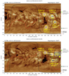 |
Fig. 6. Location of the HCS and respective CME source regions (yellow circles) overlaid on SDO/AIA 193 Å synoptic images. The HCS location is derived by the Magnetic Connectivity Tool on the basis of a PFSS (Riley et al. 2006) extrapolation for a surface height of 3Rs. The results are provided by IRAP at http://connect-tool.irap.omp.eu (see Rouillard et al. 2020). |
4. Discussion and conclusions
We analyzed two comparable episodes covering analogous solar eruptive events and their geomagnetic impacts: November 4–5 and December 1–2, 2023. The two episodes of events occurred in similar (active) regions on the Sun located near a CH. The study highlights the complexity of the heliospheric conditions during periods of interacting large-scale magnetic field structures that may lead to significant differences in geomagnetic effects.
In total eight CMEs were investigated, 2 × 4 events; the two episodes were separated by a complete solar rotation. Using stereoscopic white-light data, we reconstructed the 3D geometry, speed, and direction of motion for each CME. In addition, we derived the influence (e.g., deflection) of the nearby CH on each CME using the CHIP parameter (Gopalswamy et al. 2009). The results served as input for the CME propagation model 3D DBM (Dumbovic et al., in prep.). This allowed us to assess the impact probability of each event and to estimate their arrival times. With this we link between remote sensing image information and in situ measurements and relate them to the observed geomagnetic effects.
Relating 3D DBM model results to in situ measurements, we derive for rotation #1 a partial hit of CME1.4, while CME1.1 and CME1.2 would miss Earth, and CME1.3 would likely miss Earth. The in situ measurements reveal no obvious flux rope signature for the expected arrival time of CME1.4, but a short-lived magnetic structure presumably related to CME1.4. Two shocks are observed. While the second shock is linked to CME1.4, we speculate that the first shock might be associated with CME1.3, although this is not fully supported by the results from the 3D DBM. However, a very recent study by Gil et al. (2024) focusing on the cosmic-ray peculiarities (ACRE event) observed on November 5, 2023, came to similar conclusions. For rotation #2 we derive from 3D DBM that CME2.2 and CME2.4+5 will both hit Earth with a likely interaction between the two CMEs. From the in situ measurements two separate flux rope signatures are identified, with the clearest one connected to CME2.4+5. The shock of the fast CME2.4+5 might be located inside the ME of CME2.2 ahead.
Relating the CME signatures on the Sun to the in situ measurements, we observe for rotation #1 that the very energetic event CME1.4 corresponds to a massive filament eruption. The filament channel is found to cross the HCS which is highly tilted (i.e., oriented in the north–south direction). The source region of CME1.3 is also found to be close to the HCS. Two shocks, the first one presumably from CME1.3 and the second from CME1.4, are located ahead and behind the sector boundary. For rotation #2, we obtain that the source region of CME2.2 is near the high-tilted HCS. Moreover, for rotation #2 the SBC is embedded within the ME from CME2.2, which is close in time to the shock component of CME2.4+5 that propagated into the ME of CME2.2. A statistical study on the geomagnetic effects of shocks inside the magnetic structures of CMEs is given in Lugaz et al. (2015). Although CME1.4 only partially hits Earth, the observed stronger geomagnetic effects for rotation #1 in comparison to rotation #2 might stem from the interaction of several large-scale solar wind structures: shock-sheath components of CME1.3 and CME1.4 having strong negative Bz values combined with the SBC and related structures (see also Echer & Gonzalez 2004; Crooker et al. 2004). On the one hand, for both episodes the HCS serves as a magnetic obstacle most likely affecting CME expansion and propagation behavior. On the other hand, CMEs may play an important role in the evolution of the HCS (see recent PSP results by Romeo et al. 2023). Hence, a local reconfiguration of the HCS in interplanetary space might indeed be observed at the location where the CME flank (CME1.4) is interacting with it (see also Gil et al. 2024).
In the geomagnetic indices we observe a three-step drop–increase in Dst/Hp30 for rotation #1 and a two-step drop–increase for rotation #2. Focusing on the Dst index, we find an absolute difference between the Dst minima from rotations #1 and #2 of 55 nT. This value roughly corresponds in rotation #1 to the first Dst drop of −54 nT. That first drop in Dst is not related to any of the CMEs, but to an incoming high-density region with a rather strong negative Bz component (see also Crooker 2000). Also for rotation #2 a high-density region following a strong negative Bz component most likely contributed to the further drop in Dst. Individual HCS crossings have transition zones that might last longer than 24 hours and are related to specific magnetic structures often containing high plasma-β regions and density blobs released from the top of the helmet streamer (see, e.g., Lepping et al. 1996; Sheeley et al. 1997; Lavraud et al. 2020).
Interestingly, after each SBC we find some distinct variations (ripples) in the magnetic field regions, which are characterized as short-term structures (mesoscale range of several hours) in the total magnetic field separated by abrupt changes in the field orientation. The variations in the magnetic field are related to strongly fluctuating temperature and density profiles. These signatures could be related to i) small-scale high-density magnetic field structures due to CME-solar wind interaction (Cappello et al. 2024); ii) shock wave–magnetic field interaction, and hence compression regions (see, e.g., Pitňa et al. 2021); iii) magnetic reconnection between the CME and the HCS changing the magnetic field topology of the flux rope (e.g., Winslow et al. 2016); or iv) periodic density structures in the mesoscale range as part of the slow solar wind (Viall et al. 2021).
Concluding, the HCS together with the extended HPS, and related sector boundary crossings play an important role in the geomagnetic effects of Earth-directed CMEs. However, it is not only deflection or rotation that affects the CME when propagating near the HCS (Yurchyshyn et al. 2001; Vourlidas et al. 2011; Isavnin et al. 2014; Kay et al. 2015). For low-tilted (east–west) HCS, the “same-opposite side effect” has influence on the impact strength of CMEs (Henning et al. 1985). A lowered geoeffectiveness of CMEs is observed for events launched on the opposite side of the HCS compared to Earth (Zhao et al. 2007; Dumbović et al. 2021b). However, for a high-tilted (north–south) HCS, CMEs that are launched close to it may have an enhanced impact due to additional compression and deflection of the involved magnetic field structures. The orientation of the HCS is currently an under-represented parameter in studies relating solar activity phenomena to geomagnetic effects and might also need more attention in the applied research of space weather.
Data availability
Appendix A can be found in the following Zenodo repository.
https://wdc.kugi.kyoto-u.ac.jp/dst_provisional/; the final Dst index was not available at the time of writing.
Acknowledgments
We thank the anonymous reviewer for the instructive comments, which helped to improve the manuscript. We gratefully acknowledge the support from the Austrian-Croatian Bilateral Scientific Projects “Multi-Wavelength Analysis of Solar Rotation Profile” and “Analysis of solar eruptive phenomena from cradle to grave” under the project number OEAD HR 01/2024. M.T. and G.M.C. acknowledge support from the Young Researchers Program (YRP), project number AVO165300016. M.D., K.M. and A.K.R. acknowledge support by the Croatian Science Foundation under the project IP-2020-02-9893 (ICOHOSS). K.M., A.K.R. and F.M. acknowledge support by Croatian Science Foundation in the scope of Young Researches Career Development Project Training New Doctoral Students. F.K. and M.T. acknowledge support from the Austrian Science Fund (FWF): P 33285-N. We thank the geomagnetic observatories (Kakioka [JMA], Honolulu and San Juan [USGS], Hermanus [RSA], Alibag [IIG]), NiCT, INTERMAGNET, and many others for their cooperation to make the provisional Dst index available. This work utilizes data produced collaboratively between AFRL/ADAPT and NSO/NISP. Solar Orbiter is a space mission of international collaboration between ESA and NASA, operated by ESA. Metis was built and operated with funding from the Italian Space Agency (ASI), under contracts to the National Institute of Astrophysics (INAF) and industrial partners. Metis was built with hardware contributions from Germany (Bundesministerium für Wirtschaft und Energie through DLR), from the Czech Republic (PRODEX) and from ESA.
References
- Antonucci, E., Romoli, M., Andretta, V., et al. 2020, A&A, 642, A10 [NASA ADS] [CrossRef] [EDP Sciences] [Google Scholar]
- Arge, C., & Pizzo, V. 2000, Journal of Geophysical Research, 105, 10465 [NASA ADS] [CrossRef] [Google Scholar]
- Berdichevsky, D. B., Szabo, A., Lepping, R. P., Viñas, A. F., & Mariani, F. 2000, J. Geophys. Res., 105, 27289 [NASA ADS] [CrossRef] [Google Scholar]
- Bothmer, V., Daglis, I. A., & Bogdan, T. J. 2007, Physics Today, 60, 59 [NASA ADS] [Google Scholar]
- Brueckner, G. E., Howard, R. A., Koomen, M. J., et al. 1995, Sol. Phys., 162, 357 [NASA ADS] [CrossRef] [Google Scholar]
- Burlaga, L. F., Scudder, J. D., Klein, L. W., & Isenberg, P. A. 1990, J. Geophys. Res., 95, 2229 [NASA ADS] [CrossRef] [Google Scholar]
- Burlaga, L. F., Plunkett, S. P., & St Cyr, O. C., 2002, Journal of Geophysical Research (Space Physics), 107, 1266 [NASA ADS] [Google Scholar]
- Burlaga, L., Berdichevsky, D., Gopalswamy, N., Lepping, R., & Zurbuchen, T. 2003, Journal of Geophysical Research (Space Physics), 108, 1425 [NASA ADS] [Google Scholar]
- Cappello, G. M., Temmer, M., Vourlidas, A., et al. 2024, A&A, 688, A162 [NASA ADS] [CrossRef] [EDP Sciences] [Google Scholar]
- Cargill, P. J. 2004, Solar Physics, 221, 135 [NASA ADS] [CrossRef] [Google Scholar]
- Cliver, E. W., & Svalgaard, L. 2004, Sol. Phys., 224, 407 [NASA ADS] [CrossRef] [Google Scholar]
- Cole, K. D. 1965, J. Geophys. Res., 70, 1689 [NASA ADS] [CrossRef] [Google Scholar]
- Cranmer, S. R., Gibson, S. E., & Riley, P. 2017, Space Science Reviews, 212, 1345 [NASA ADS] [CrossRef] [Google Scholar]
- Crooker, N. U. 2000, Journal of Atmospheric and Solar-Terrestrial Physics, 62, 1071 [NASA ADS] [CrossRef] [Google Scholar]
- Crooker, N. U., Huang, C. L., Lamassa, S. M., et al. 2004, Journal of Geophysical Research (Space Physics), 109, A03107 [NASA ADS] [Google Scholar]
- De Leo, Y., Burtovoi, A., Teriaca, L., et al. 2023, A&A, 676, A45 [NASA ADS] [CrossRef] [EDP Sciences] [Google Scholar]
- Dissauer, K., Veronig, A. M., Temmer, M., & Podladchikova, T. 2019, ApJ, 874, 123 [NASA ADS] [CrossRef] [Google Scholar]
- Dumbović, M., Devos, A., Vršnak, B., et al. 2015, Sol. Phys., 290, 579 [Google Scholar]
- Dumbović, M., Guo, J., Temmer, M., et al. 2019, ApJ, 880, 18 [Google Scholar]
- Dumbović, M., Čalogović, J., Martinić, K., et al. 2021a, Frontiers in Astronomy and Space Sciences, 8 [Google Scholar]
- Dumbović, M., Veronig, A. M., Podladchikova, T., et al. 2021b, A&A, 652, A159 [NASA ADS] [CrossRef] [EDP Sciences] [Google Scholar]
- Echer, E., & Gonzalez, W. D. 2004, Geophys. Res. Lett., 31, L09808 [NASA ADS] [Google Scholar]
- Echer, E., Gonzalez, W. D., Tsurutani, B. T., & Gonzalez, A. L. C. 2008, Journal of Geophysical Research (Space Physics), 113, A05221 [NASA ADS] [Google Scholar]
- Fenrich, F. R., & Luhmann, J. G. 1998, Geophys. Res. Lett., 25, 2999 [NASA ADS] [CrossRef] [Google Scholar]
- Fineschi, S., Naletto, G., Romoli, M., et al. 2020, Experimental Astronomy, 49, 239 [NASA ADS] [CrossRef] [Google Scholar]
- Geyer, P., Dumbović, M., Temmer, M., et al. 2023, A&A, 672, A168 [NASA ADS] [CrossRef] [EDP Sciences] [Google Scholar]
- Gil, A., Asvestari, E., Mishev, A., Larsen, N., & Usoskin, I. 2024, Solar Physics, 299, 9 [NASA ADS] [CrossRef] [Google Scholar]
- Gopalswamy, N., Yashiro, S., Kaiser, M. L., Howard, R. A., & Bougeret, J. L. 2001, ApJ, 548, L91 [NASA ADS] [CrossRef] [Google Scholar]
- Gopalswamy, N., Mäkelä, P., Xie, H., Akiyama, S., & Yashiro, S. 2009, Journal of Geophysical Research (Space Physics), 114, A00A22 [NASA ADS] [Google Scholar]
- Guo, J., Dumbović, M., Wimmer-Schweingruber, R. F., et al. 2018, Space Weather, 16, 1156 [NASA ADS] [CrossRef] [Google Scholar]
- Hajra, R., Tsurutani, B. T., & Lakhina, G. S. 2020, ApJ, 899, 3 [NASA ADS] [CrossRef] [Google Scholar]
- Heinemann, S. G., Temmer, M., Farrugia, C. J., et al. 2019a, Solar Physics, 294, 1 [NASA ADS] [CrossRef] [Google Scholar]
- Heinemann, S. G., Temmer, M., Heinemann, N., et al. 2019b, Sol. Phys., 294, 144 [NASA ADS] [CrossRef] [Google Scholar]
- Heinemann, S. G., Jerčić, V., Temmer, M., et al. 2020, A&A, 638, A68 [EDP Sciences] [Google Scholar]
- Henning, H. M., Scherrer, P. H., & Hoeksema, J. T. 1985, J. Geophys. Res., 90, 11055 [NASA ADS] [CrossRef] [Google Scholar]
- Hoeksema, J. T., Wilcox, J. M., & Scherrer, P. H. 1983, J. Geophys. Res., 88, 9910 [CrossRef] [Google Scholar]
- Howard, R. A., Moses, J. D., Vourlidas, A., et al. 2008, Space Sci. Rev., 136, 67 [NASA ADS] [CrossRef] [Google Scholar]
- Isavnin, A., Vourlidas, A., & Kilpua, E. K. J. 2014, Sol. Phys., 289, 2141 [NASA ADS] [CrossRef] [Google Scholar]
- Kaiser, M. L., Kucera, T. A., Davila, J. M., et al. 2008, Space Sci. Rev., 136, 5 [Google Scholar]
- Kay, C., Opher, M., & Evans, R. M. 2015, ApJ, 805, 168 [NASA ADS] [CrossRef] [Google Scholar]
- King, J. H., & Papitashvili, N. E. 2020, OMNI 1-min Data Set [Google Scholar]
- Kozyra, J. U., & Liemohn, M. W. 2003, Space Sci. Rev., 109, 105 [NASA ADS] [CrossRef] [Google Scholar]
- Lavraud, B., Fargette, N., Réville, V., et al. 2020, ApJ, 894, L19 [Google Scholar]
- Lemen, J. R., Title, A. M., Akin, D. J., et al. 2012, Sol. Phys., 275, 17 [Google Scholar]
- Lepping, R. P., Szabo, A., Peredo, M., & Hoeksema, J. T. 1996, Geophys. Res. Lett., 23, 1199 [NASA ADS] [CrossRef] [Google Scholar]
- Lugaz, N., Manchester, W. B., I, & Gombosi, T. I. 2005, ApJ, 634, 651 [NASA ADS] [CrossRef] [Google Scholar]
- Lugaz, N., Farrugia, C. J., Smith, C. W., & Paulson, K. 2015, Journal of Geophysical Research (Space Physics), 120, 2409 [NASA ADS] [CrossRef] [Google Scholar]
- Lugaz, N., Farrugia, C. J., Winslow, R. M., et al. 2016, Journal of Geophysical Research (Space Physics), 121, 861 [NASA ADS] [Google Scholar]
- Lugaz, N., Temmer, M., Wang, Y., & Farrugia, C. J. 2017, Solar Physics, 292 [CrossRef] [Google Scholar]
- Mäkelä, P., Gopalswamy, N., Xie, H., et al. 2013, Sol. Phys., 284, 59 [CrossRef] [Google Scholar]
- Manchester, W., Kilpua, E. K. J., Liu, Y. D., et al. 2017, Space Sci. Rev., 212, 1159 [Google Scholar]
- McComas, D. J., Angold, N., Elliott, H. A., et al. 2013, ApJ, 779, 2 [Google Scholar]
- Müller, D., St. Cyr, O. C., Zouganelis, I., et al. 2020, A&A, 642, A1 [Google Scholar]
- Owens, M. J., Chakraborty, N., Turner, H., et al. 2022, Sol. Phys., 297, 83 [NASA ADS] [CrossRef] [Google Scholar]
- Palmerio, E., Kilpua, E. K. J., Möstl, C., et al. 2018, Space Weather, 16, 442 [NASA ADS] [CrossRef] [Google Scholar]
- Patsourakos, S., & Vourlidas, A. 2012, Sol. Phys., 281, 187 [NASA ADS] [Google Scholar]
- Pesnell, W. D., Thompson, B. J., & Chamberlin, P. C. 2012, Sol. Phys., 275, 3 [Google Scholar]
- Pitňa, A., Šafránková, J., Němeček, Z., Ďurovcová, T., & Kis, A. 2021, Frontiers in Physics, 8, 654 [Google Scholar]
- Riley, P., Linker, J. A., Mikić, Z., et al. 2006, ApJ, 653, 1510 [Google Scholar]
- Romeo, O. M., Braga, C. R., Badman, S. T., et al. 2023, ApJ, 954, 168 [NASA ADS] [CrossRef] [Google Scholar]
- Rouillard, A. P., Pinto, R. F., Vourlidas, A., et al. 2020, A&A, 642, A2 [NASA ADS] [CrossRef] [EDP Sciences] [Google Scholar]
- Russell, C. T., & Mulligan, T. 2002, Planet. Space Sci., 50, 527 [Google Scholar]
- Scherrer, P. H., Schou, J., Bush, R. I., et al. 2012, Sol. Phys., 275, 207 [Google Scholar]
- Scolini, C., Chané, E., Pomoell, J., Rodriguez, L., & Poedts, S. 2020, Space Weather, 18 [CrossRef] [Google Scholar]
- Sheeley, N. R., Wang, Y. M., Hawley, S. H., et al. 1997, ApJ, 484, 472 [Google Scholar]
- Smith, E. J. 2001, J. Geophys. Res., 106, 15819 [NASA ADS] [CrossRef] [Google Scholar]
- Temmer, M., Reiss, M. A., Nikolic, L., Hofmeister, S. J., & Veronig, A. M. 2017, The Astrophysical Journal, 835, 1 [Google Scholar]
- Temmer, M., Scolini, C., Richardson, I. G., et al. 2023, Advances in Space Res., in press [arXiv:2308.04851] [Google Scholar]
- Temmer, M., Vršnak, B., Rollett, T., et al. 2012, ApJ, 749, 57 [NASA ADS] [CrossRef] [Google Scholar]
- Thernisien, A. 2011, ApJS, 194, 33 [Google Scholar]
- Thernisien, A. F., Morrill, J. S., Howard, R. A., & Wang, D. 2006, Solar Physics, 233, 155 [NASA ADS] [CrossRef] [Google Scholar]
- Tsurutani, B. T., Zank, G. P., Sterken, V. J., et al. 2023, IEEE Transactions on Plasma Science, 51, 1595 [NASA ADS] [CrossRef] [Google Scholar]
- Turner, N. E., Baker, D. N., Pulkkinen, T. I., et al. 2001, J. Geophys. Res., 106, 19149 [NASA ADS] [CrossRef] [Google Scholar]
- Verbeke, C., Mays, M. L., Kay, K., et al. 2023, Advances in Space Research, 72, 5243 [NASA ADS] [CrossRef] [Google Scholar]
- Viall, N. M., DeForest, C. E., & Kepko, L. 2021, Frontiers in Astronomy and Space Sciences, 8, 139 [NASA ADS] [CrossRef] [Google Scholar]
- Vourlidas, A., Colaninno, R., Nieves-Chinchilla, T., & Stenborg, G. 2011, ApJ, 733, L23 [NASA ADS] [CrossRef] [Google Scholar]
- Vršnak, B., Temmer, M., & Veronig, A. M. 2007, Sol. Phys., 240, 315 [Google Scholar]
- Vršnak, B., Žic, T., Vrbanec, D., et al. 2013, Solar Physics, 285, 295 [CrossRef] [Google Scholar]
- Vršnak, B., Temmer, M., Žic, T., et al. 2014, ApJS, 213, 21 [CrossRef] [Google Scholar]
- Winslow, R. M., Lugaz, N., Schwadron, N. A., et al. 2016, Journal of Geophysical Research (Space Physics), 121, 6092 [NASA ADS] [CrossRef] [Google Scholar]
- Winslow, R. M., Scolini, C., Lugaz, N., & Galvin, A. B. 2021, ApJ, 916, 40 [NASA ADS] [CrossRef] [Google Scholar]
- Winterhalter, D., Smith, E. J., Burton, M. E., Murphy, N., & McComas, D. J. 1994, J. Geophys. Res., 99, 6667 [NASA ADS] [CrossRef] [Google Scholar]
- Wu, C.-C., Liou, K., Lepping, R. P., et al. 2017, Sol. Phys., 292, 109 [NASA ADS] [CrossRef] [Google Scholar]
- Yamazaki, Y., Matzka, J., Stolle, C., et al. 2022, Geophysical Research Letters, 49, e2022GL098860 [CrossRef] [Google Scholar]
- Yordanova, E., Temmer, M., Dumbovié, M., Space, et al. 2024, Weather, 22, e2023SW003497 [NASA ADS] [CrossRef] [Google Scholar]
- Yurchyshyn, V. B., Wang, H., Goode, P. R., & Deng, Y. 2001, ApJ, 563, 381 [NASA ADS] [CrossRef] [Google Scholar]
- Zhang, J., Temmer, M., Gopalswamy, N., et al. 2021, Progress in Earth and Planetary Science, 8, 56 [NASA ADS] [CrossRef] [Google Scholar]
- Zhao, X., Feng, X., & Wu, C.-C. 2007, Journal of Geophysical Research (Space Physics), 112, A06107 [NASA ADS] [Google Scholar]
Appendix B: 3D DBM modeling of the CME-CME interaction
3D DBM tracks the kinematics of the infinitesimally thin leading edge of the CME. The interaction of two CMEs in 3D DBM can therefore be approximated as a trailing front encountering the leading front. We note that in reality this is not the case, because the front of the trailing CME first interacts with the back of the leading CME. Nevertheless, this approach offers a simple and fast way to treat CME-CME interactions with 3D DBM. We consider the point where the kinematic curves of two CMEs cross as the interaction point. We assume that during the interaction impulse and mass are conserved and that after the interaction the two CMEs move on as a single entity. The initial parameters are then recalculated for the entity at the interaction point (starting time, starting distance, speed based on conserved momentum, γ parameter), with the solar wind speed slightly enhanced. The γ parameter is recalculated based on the increased CME leading front cross sectional area and mass (for details see Guo et al. 2018; Dumbović et al. 2019):
 (B.1)
(B.1)
Here γ1 is the original γ parameter of the first CME,  is the mass ratio of the two CMEs (estimated roughly by the observer, based on the impulsiveness, brightness and spatial extent of the two CMEs in the white light observations), ω1 is the spatial extent of the first CME (estimated as the extent in either equatorial or meridional plane, whichever is larger), and ω1 + 2 is the extent of the merged CME entity, which is derived by combining the extents of both CMEs in equatorial and meridional planes and choosing whichever is larger. The extent (half-width) of the entity in equatorial plane is calculated as
 (B.2)
(B.2)
where ω stands for half-width, lon for longitude and indices max and min correspond to wider and narrower CME in the interaction, respectively. An analogous equation is used to calculate the half-width of the entity in the meridional plane.
The original drag parameters corresponding to CMEs before interaction are calculated according to Cargill (2004) and Vršnak et al. (2014) as
 (B.3)
(B.3)
where we assume Cd equals 1, r is the radius of the CME, which has toroidal geometry and is calculated according to Thernisien (2011). The density ratio n/nSW is estimated based on the CME speed, using the CME mass vs. speed relation (see Table 1 in Dissauer et al. 2019) and typical values for density ratio used in the ENLIL cone model (see, e.g., Yordanova et al. 2024), grouping CMEs into three classes: slow (< 750 km/s), intermediate (750–1500 km/s) and fast (> 1500 km/s). For intermediate CMEs we use density ratio 4 (typical value used in ENLIL cone). For slow and fast CMEs with masses ≈ 2 times smaller and 1.5 times larger than for intermediate CMEs, respectively, we use density ratios of 2 and 6, respectively.
All Tables
All Figures
|
Fig. 1. General overview of the CME occurrence and CHs for the two episodes, rotation #1 (left panel) and rotation #2 (right panel), overlaid on AIA 193 Å images. Given are the CH locations with their center of mass (CM) and apex distances to the active regions (AR) from which the CMEs were launched (see details in Sect. 2.1). For each CME the 3D speed information is given as derived from a linear fit to sequential GCS reconstructions. For rotation #1 we observe four CMEs (CME1.1–1.4) and for rotation #2 five CMEs (CME2.1–2.4+5). We note that for CME 2.1 the corresponding active region is already behind the western limb, and therefore no AR distance is given. The image dates were chosen such that the CH is centrally located for better visibility. |
| In the text | |
|
Fig. 2. Overview of the eruption sites and CME cone projections. Top panels: SDO/AIA EUV composite ratio images (source: suntoday.lmsal.com) for each eruptive event. Bottom panels: CME cone geometry derived from GCS results (longitude, latitude, tilt) projected on the ecliptic and meridional plane. The events are annotated with the eruption related GOES SXR flare classes. Left panels: Rotation #1 over the period from 2023-10-31 21:27 UT to 2023-11-03 05:52 UT. CME1.1+1.2+1.4 are related to filament eruptions f1+f2+f3, respectively. Right panels: rotation #2 over the period 2023-11-27 18:48 UT until 2023-11-28 19:50 UT. CME2.1+2.4 are related to filament eruptions f1+f2, respectively. |
| In the text | |
|
Fig. 3. For rotation #1 we show on the example of CME1.2 the CME structure from different perspectives (LASCO C2, COR2, and Metis) and GCS reconstruction for the CME at a 3D height of 5.4Rs. Bottom right panel: from different time steps the height-time and speed are derived using a linear fit (given in the legend). |
| In the text | |
|
Fig. 4. For rotation #2 we show on the example of CME2.3 the CME structure from different perspectives (LASCO C2, COR2, and Metis) and GCS reconstruction for the CME at a 3D height of 13.0 Rs. Bottom right panel: from different time steps the height-time and speed are derived using a linear fit (given in the legend). |
| In the text | |
|
Fig. 5. OMNI in situ measurements and geomagnetic indices for each rotation (x-axis shows time in UT). From top to bottom: magnetic field and vector components, density+temperature, plasma-β+speed, Dst+Hp30. Shown are a high plasma-β structure heliospheric plasma sheet (HB), high-density (HD) structures, the shocks (SH; dashed vertical lines) from various CMEs, the sector boundary crossing (SBC; dotted red vertical line), magnetic ejecta (ME) related to the different CMEs, and the start of the SIR/HSS (gray shaded area marks the interaction zone between the rear-part of the CME and the starting of the SIR). The red arrows indicate the observed ripples (short-term variations in the total magnetic field associated with strong fluctuations in the temperature and density profiles). A zoomed-in image for the regions around the SBC is shown in Fig. A.7. |
| In the text | |
|
Fig. 6. Location of the HCS and respective CME source regions (yellow circles) overlaid on SDO/AIA 193 Å synoptic images. The HCS location is derived by the Magnetic Connectivity Tool on the basis of a PFSS (Riley et al. 2006) extrapolation for a surface height of 3Rs. The results are provided by IRAP at http://connect-tool.irap.omp.eu (see Rouillard et al. 2020). |
| In the text | |
Current usage metrics show cumulative count of Article Views (full-text article views including HTML views, PDF and ePub downloads, according to the available data) and Abstracts Views on Vision4Press platform.
Data correspond to usage on the plateform after 2015. The current usage metrics is available 48-96 hours after online publication and is updated daily on week days.
Initial download of the metrics may take a while.