| Issue |
A&A
Volume 694, February 2025
|
|
|---|---|---|
| Article Number | A152 | |
| Number of page(s) | 13 | |
| Section | Stellar structure and evolution | |
| DOI | https://doi.org/10.1051/0004-6361/202452920 | |
| Published online | 11 February 2025 | |
Searching for Galactic red supergiants with Gaia RVS spectra
1
Institute for Frontiers in Astronomy and Astrophysics, Beijing Normal University, Beijing 102206, People’s Republic of China
2
School of Physics and Astronomy, Beijing Normal University, Beijing 100875, People’s Republic of China
3
College of Physics and Electronic Engineering, Qilu Normal University, Jinan 250200, People’s Republic of China
4
Purple Mountain Observatory and Key Laboratory of Radio Astronomy, Chinese Academy of Sciences, 10 Yuanhua Road, Nanjing 210033, People’s Republic of China
5
Key Laboratory of Space Astronomy and Technology, National Astronomical Observatories, Chinese Academy of Sciences, Beijing 100101, People’s Republic of China
⋆ Corresponding author; bjiang@bnu.edu.cn
Received:
7
November
2024
Accepted:
19
December
2024
Red supergiants (RSGs) are essential to understanding the evolution and the contribution to the interstellar medium of massive stars. However, the number of identified RSGs within the Milky Way is still limited, mainly due to the difficulty of measuring stellar extinction and distance. The release of approximately one million RVS spectra in Gaia DR3 presents a new opportunity for identifying Galactic RSGs because the equivalent width of the calcium triplet lines (EW(CaT)) in the spectra is an excellent indicator of stellar surface gravity. We used RVS spectra with a signal-to-noise ratio (S/N) greater than 100 to search for Galactic RSGs. We removed dwarf stars and red giants and selected RSG candidates based on their location in the EW(CaT) versus BP − RP diagram. Early-type RSG candidates (K0-M2) were then identified using the criteria BP − RP > 1.584 and EW(CaT) > 1.1 nm. The criteria of the average equivalent widths of TiO in the XP spectra (EW(TiO)) > 10 nm, the color index K − W3 < 0.5, and the period-amplitude sequence from the Gaia DR3 LPV catalog were further applied to remove late-type red giants (after M2) and asymptotic giant branch stars. This method yielded 30 early-type (K0-M2) and 6196 late-type (after M2) RSG candidates, which is a significant increase compared to the previous Galactic RSG sample. The application of this approach to spectra with S/N > 50 resulted in 48 early-type and 11 491 late-type RSG candidates. This preliminary analysis paves the way for more extensive research with Gaia DR4, when larger spectral datasets are expected to significantly enhance our understanding of Galactic RSG populations.
Key words: stars: late-type / stars: massive / supergiants
© The Authors 2025
 Open Access article, published by EDP Sciences, under the terms of the Creative Commons Attribution License (https://creativecommons.org/licenses/by/4.0), which permits unrestricted use, distribution, and reproduction in any medium, provided the original work is properly cited.
This article is published in open access under the Subscribe to Open model. Subscribe to A&A to support open access publication.
1. Introduction
Red supergiants (RSGs) are among the most massive and luminous stars in the Universe, representing a crucial evolutionary phase for stars with initial masses between approximately 8 and 40 M⊙ (Humphreys & Davidson 1979; Massey & Olsen 2003). RSGs are characterized by their immense size, cool temperature, complex light variability (Kiss et al. 2006; Yang & Jiang 2012; Ren et al. 2019; Ren & Jiang 2020; Zhang et al. 2024), and significant mass-loss rate (Humphreys et al. 2020; Beasor et al. 2020; Wang et al. 2021; Yang et al. 2023; Wen et al. 2024; Decin et al. 2024), which have profound affects for their subsequent evolution and eventual fate as supernovae.
Attempts to identify RSGs in nearby galaxies have recently made great progress thanks to new observations and the fast development of new methods. In the Small and Large Magellanic Clouds (SMC and LMC), the parallax, proper motions, and radial velocity (RV) measured by Gaia are highly reliable parameters that can be used to select member stars (Yang et al. 2019; Ren et al. 2021b). Though the Gaia astrometric parameters are sufficiently accurate to select member stars, they are unavailable for most stars in galaxies more distant than the SMC and LMC because of Gaia’s limited sensitivity. The color–color diagram method was thus invented to select member stars. A very early attempt was carried out by Massey (1998). They used the B − V/V − R diagram to separate the foreground dwarf stars from member giant stars because the B band covers some metallic lines sensitive to surface gravity. Ren et al. (2021a) improved upon this method by shifting the waveband to the near-infrared (NIR) J − H/H − K diagram. The NIR color–color diagram has the advantages of being consistent with the peak of the RSG spectral energy distribution and being much less affected by interstellar extinction. After the foreground stars are removed, RSGs in an external galaxy can be easily identified by their high luminosity and red color in the color-magnitude diagram since all member stars are at almost the same distance. Consequently, 5498 and 3055 RSGs have been identified in M31 and M33 (Ren et al. 2021a), 4823 and 2138 RSGs in the LMC and SMC, and a total of 2190 RSGs in another ten dwarf galaxies (Ren et al. 2021b).
The identification of RSGs in the Galaxy lags behind. The Galactic RSGs are distributed in various directions and distances, so no identical proper motion, parallax, or RV can be used. Thus, astrophysical parameters such as luminosity and color index should be determined to find RSGs. However, inhomogeneous and heavy extinction renders the measurement of both luminosity and intrinsic color index difficult (e.g., Schödel et al. 2010) because RSGs are located in the Galactic plane. Besides, the distance should be measured individually, and the perturbation of the photocenter of RSGs adds additional uncertainty to the Gaia parallax (Chiavassa et al. 2011). Instead of photometry, the identification of RSGs in the Galaxy relies heavily on spectroscopy. The very early identification of RSGs in nearby galaxies also used spectral features and the RVs derived from spectra (see, e.g., Humphreys et al. 1988).
A spectrum contains abundant information for stellar classification. In particular, NIR spectra are suitable for late-type stars (Kirkpatrick et al. 1991; Ginestet et al. 1994; Carquillat et al. 1997). Based on the spectral classifications by Humphreys (1978) and Garmany & Stencel (1992), Levesque et al. (2005) built a catalog of 74 Galactic RSGs, including their spectral types and effective temperature scales. Additionally, attention has been directed toward star clusters within the Milky Way, as RSGs are often found within OB associations. There are three massive RSG-rich clusters named RSGC1, RSGC2, and RSGC3 located in a small region of the Galactic plane between l = 24° and l = 29° (Figer et al. 2006; Davies et al. 2007, 2008; Clark et al. 2009; Alexander et al. 2009), as well as several smaller clusters close to them (Negueruela et al. 2010, 2011, 2012). In a more recent study, Dorda et al. (2016) used principal component analysis and support vector machine techniques to analyze the spectral features in the calcium triplet (CaT) region, establishing the criteria for distinguishing supergiants from non-supergiants. They subsequently applied this method to identify 197 cool supergiants in the Perseus arm (Dorda et al. 2018). Messineo & Brown (2019) selected Galactic K-M type Class I stars and identified 889 RSG candidates using Gaia Data Release (DR) 2 astrometric data, but only a small fraction of them have been confirmed as true RSGs. Furthermore, Messineo (2023) identified 20 new RSGs through an analysis of Gaia DR3 General Stellar Parametrizer from photometry (GSP-Phot) and General Stellar Parametrizer from spectroscopy (GSP-Spec) parameters in combination with blue and red prism spectra (BP and RP, respectively). More recently, Healy et al. (2024) compiled a catalog of 578 highly probable and 62 likely RSGs. Despite the Milky Way being estimated to host at least 5000 RSGs (Gehrz 1989), the currently known sample is far smaller. This discrepancy is mainly due to the limitations of spectroscopic surveys, which typically detect only bright sources. Spectroscopy is also generally less efficient than photometry. Fortunately, Gaia DR3 includes a vast number of medium-resolution Radial Velocity Spectrometer (RVS) spectra (Sartoretti et al. 2018, 2023; Recio-Blanco et al. 2023). Additionally, space observations avoid the absorption lines of the atmosphere, which improves the accuracy of line measurements. It offers an unprecedented opportunity to revisit the population of Galactic RSGs from a new perspective.
This work aims to create a large catalog of Galactic RSGs through a comprehensive analysis of RVS spectra. The paper is organized as follows: Section 2 introduces the RVS spectra and the process of re-normalization, as well as the selection of the initial sample. Section 3 describes the CaT characteristics of preliminary RSG samples and the processes for selecting early-type and late-type RSG candidates. We discuss the known Galactic RSGs, completeness, and pureness in our sample, and present an outlook for Gaia DR4 in Sect. 4. A summary is presented in Sect. 5.
2. Data
2.1. RVS spectra
Launched by the European Space Agency in 2013, the Gaia mission aims to create the most detailed three-dimensional map of our galaxy. Gaia’s suite of instruments includes a highly precise astrometric detector, photometric facility, and the RVS (Gaia Collaboration 2016). The RVS is designed to obtain medium-resolution spectra in the wavelength range of 845–872 nm (Sartoretti et al. 2018), also known as CaT region, which is suitable to determine the RV over a wide range of metallicity. This spectral region is very valuable for studying cool stars like RSGs, as it contains strong absorption lines that are sensitive to temperature, surface gravity, and metallicity (Contursi et al. 2021; Creevey et al. 2023; Fouesneau et al. 2023), in particular, CaT itself is an excellent indicator of surface gravity (Diaz et al. 1989; Mallik 1994, 1997; Cenarro et al. 2001a,b).
Gaia DR3 includes 999 645 RVS spectra with a resolution of R ∼ 11 150. These spectra are wavelength-calibrated under vacuum conditions, and the majority has a signal-to-noise ratio (S/N) between 20 and 40 (Gaia Collaboration 2023b). They are primarily used for measuring stellar RV (Katz et al. 2023) or for deriving GSP-Spec parameters with the Apsis pipeline (Creevey et al. 2023; Fouesneau et al. 2023; Recio-Blanco et al. 2023). The RVS spectra cover the features for a wide range of stellar types, with early-type stars dominated by hydrogen Paschen lines, while late-type stars exhibit more metallic and molecular lines (see Fig. 6 of Fouesneau et al. 2023). The publicly released RVS spectra are normalized either by using their pseudo-continuum or by scaling with a constant (the latter for cool stars or low-S/N spectra; Gaia Collaboration 2023b). For the majority of stars, the normalized flux is set to 1. However, due to the presence of the TiO band in the spectra of late-type stars that erode the pseudo-continuum, the normalization process is often incorrect for M-type stars. As a result, their spectra exhibit a pronounced slope across the entire wavelength range (e.g., Fig. 17 in Cropper et al. 2018). Given that Galactic RSGs are mostly of M-type (see Fig. 5 of Levesque & Massey 2012), it is necessary to re-normalize the spectra.
The steps for continuum re-normalization are as follows. First, the spectral regions with no apparent absorption bands are selected, indicated by red points in Fig. 1, ignoring the narrow atomic lines listed in Dorda et al. (2016). Then, a linear fitting is performed to these points, and the original spectrum is divided by this fitting line to get the re-normalized spectrum. At last, the continuum of the spectrum is defined as the Gaussian mean of the points used for the linear fitting to correct for possible systematic offset. Figure 1 shows an example of this process, with the CaT measurement region marked in green. For consistency, the re-normalization is applied to all spectra, and the spectra of late-type stars are effectively flattened, while no significant difference is observed in the spectra of other-type stars before and after the correction.
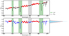 |
Fig. 1. Example of RVS spectrum re-normalization (source_id: 5836392511305856128). The upper panel shows the original spectrum, and the solid red line is obtained via linear fitting of the red dots. The blue on the bottom panel is the re-normalized spectrum, the histogram on the lower right is a distribution of red dots, and the dashed black line marks the mean of its Gaussian fitting, representing the continuum after re-normalization. The shaded colors are used to represent different absorption lines. |
2.2. Selection of the initial sample of Galactic stars
2.2.1. Data preprocessing
To ensure that the analyzed spectra are from Galactic stars, the following criteria are applied:
-
A stellar probability greater than 99% (classprob_dsc_combmod_star> 0.99);
-
Stars not located in the LMC (i.e., stars within the region 64° < RA < 98°, −78° < Dec. < −59° and with RVs greater than 100 km/s are excluded);
-
Stars not located in the SMC (i.e., stars within the region 2° < RA < 26°, −76° < Dec. < −69° and with RVs greater than 100 km/s are excluded);
As a result, 7407 spectra were excluded. From the remaining spectra, only those with a S/N greater than 100 (rvs_spec_sig_to_noise > 100) were chosen. This was done to ensure that the subsequent analysis is performed on high-quality spectra, minimizing the impact of noise on the equivalent width measurements. In the end, 118 048 spectra were retained for further analysis.
2.2.2. Removal of early-type stars
Because the Paschen series lines P13, P15, and P16 in early-type stars appear at similar wavelengths as the CaT (see Fig. 2), the measurement of the EW(CaT) may be actually conducted to the hydrogen lines. Thus, it is necessary to remove the early-type stars.
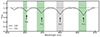 |
Fig. 2. Example of the RVS spectrum of a typical early-type star (source_id: 2270570062017774976). The position indicated by the arrow marks the Paschen line series P13-P16 for hydrogen. The gray and green shade mark the measuring ranges of P14 and CaT, respectively. |
Since no strong absorption lines in the spectra of late-type stars appear near P14 (see Fig. 2), the equivalent width of P14 region (EW(P14)) is used as the diagnosis of early-type stars. EW(P14) is calculated by using the equivalent_width function from the specutils package (Astropy-Specutils Development Team 2019). The continuum is determined by using the Gaussian mean of the points for the linear fitting described in Sect. 2.1, which is shown by the dashed black line in Fig. 2 where the continuum level is 1.013 in this case. The wavelength range is set between 859 and 861 nm (i.e., the shaded gray region in Fig. 2).
In addition to the EW(P14), the slope of the original Gaia RVS continuum derived from the linear fitting in Sect. 2.1 is supplemented to assure the identification of early-type stars. Because the continuum of early-type stars are not affected by broad molecular bands, the slope should be small. As shown in Fig. 3, stars with significant EW(P14) indeed exhibit a small continuum slope, which supports this criterion. Specifically, stars with EW(P14) greater than 0.1 nm and a slope less than 0.0025 are classified as early-type. Consequently, a total of 12 396 stars are excluded, which are located in the dashed black box in Fig. 3. Among the initial 118 048 stars in the sample, 8157 have available teff_esphs values, indicating temperatures above 7500 K, and are thus considered hot stars (Creevey et al. 2023). Notably, of the 12 396 early-type stars excluded, 8133 (∼99.7%) fall within this group, further validating the effectiveness of the early-type star identification and exclusion process.
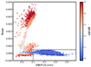 |
Fig. 3. Diagram used to remove early-type stars. The horizontal and vertical axes are EW(P14) and the slope mentioned in Sect. 2.1, respectively. The dashed black box defines the area of early-type stars, and the dots are color-coded by BP − RP. |
3. The Galactic RSG candidates
The RSG candidates are basically selected by the EW(CaT) in that it is generally larger for supergiants than dwarfs or giants. However, the Galactic RSGs are mostly M-type (Levesque & Massey 2012), leading to the decrease in EW(CaT) to be comparable to that of giants or even dwarfs (Jennings & Levesque 2016). Thus, other parameters, including the color index BP − RP and K − W3 and the equivalent width of TiO band, are taken into account. Accordingly, the RSG candidates are divided into the early-type (K0-M2) and late-type (after M2) groups during the process.
3.1. Preliminary sample of RSGs in the EW(CaT) versus BP − RP diagram
3.1.1. EW(CaT) of RSGs
The CaT is a characteristic absorption feature in the NIR spectrum, with wavelengths centered at 8498, 8542, and 8662 Å in air (see, e.g., Contursi et al. 2021; Creevey et al. 2023; Fouesneau et al. 2023). It serves as a strong indicator of luminosity class (i.e., surface gravity), where lower surface gravity typically corresponds to stronger CaT absorption, resulting in a larger EW(CaT). Therefore, using EW(CaT) to identify RSGs is a reasonable approach, and this has been applied in previous studies. Humphreys et al. (1988) classified stars with EW(CaT) greater than 1.1 nm as supergiants when analyzing RSG spectra in M31. Negueruela et al. (2011), focusing only on the 8542 and 8662 Å lines, found that Galactic RSGs earlier than M3 satisfied EW(Ca II 8542 + Ca II 8662) > 0.9 nm. Within the same luminosity class, EW(CaT) increases from F- or G-type stars until it saturates at around M2, after which it rapidly decreases with later spectral type. This decline is due to the increasing prominence of TiO in late-type stars, which erodes both the continuum and atomic lines, thus reducing the equivalent width of CaT.
Although this trend has been proved in previous studies (see Fig. 4 in Negueruela et al. 2011 and Fig. 9 in Dorda et al. 2016), 185 known Galactic RSGs are selected to quantitatively examine the variation of EW(CaT) with spectral type. Their EW(CaT) measurements are taken from Cesetti et al. (2013), Dorda et al. (2018), Dicenzo & Levesque (2019), or this work with RVS spectra. Figure 4 illustrates the relation between EW(CaT) and spectral type for these stars, displaying the same trend as previously described. Early-type RSGs (up to M2) have EW(CaT) > 1.1 nm, which is consistent with the definition by Humphreys et al. (1988). In Fig. 4, the EW(CaT) value at M6 has a large dispersion, which is because of the difficulties in determining the spectral type of late-M RSGs, as they are variable. For instance, the star with the largest EW(CaT) at M6 is the well-known NML Cyg, whose spectral type is reported to range from M4.5 to M7.9 (Samus’ et al. 2017). NML Cyg is a supergiant, potentially even a hypergiant, and its EW(CaT) is expected to be larger than that of stars with similar spectral types. Conversely, the star with the smallest EW(CaT) at M6 is V577 Cep, whose spectral type is reported to range from M6 to M8 (Skiff 2014). Nakamura et al. (2016) included V577 Cep in their catalog of nearby RSG candidates, although they claimed the possibility that their sample may contain red giants with luminosity class of II or III. A linear fitting is applied to build the relation of EW(CaT) with spectral type later than M2, requiring the fitting to pass through the M2 type at EW(CaT) = 1.1 nm, as shown by the black line in Fig. 4. This provides an approximate EW(CaT) values for RSGs of later spectral types, which is listed in Table 1. It can be noted that the EW(CaT) decreases to 0.230 nm at M8.
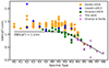 |
Fig. 4. Spectral types vs. EW(CaT) for 185 known Galactic RSGs, with their EW(CaT) measurements from Cesetti et al. (2013), Dorda et al. (2018), and Dicenzo & Levesque (2019). For the only magenta asterisk, the results of Dorda et al. (2018) and Dicenzo & Levesque (2019) are represented after being averaged. The crosses denote the sources measured in this work from the Gaia RVS spectra. The solid black lines mark EW(CaT) = 1.1 nm (for K-type or early M-type RSGs) and the decreasing of EW(CaT) with spectral type (for RSGs later than M2). |
3.1.2. (BP − RP)0 of RSGs
The intrinsic color index (BP − RP)0 was calculated to constrain the minimal observational BP − RP for a specific subtype that is associated with the EW(CaT). In addition, RSGs are usually more luminous than other type of stars and experience higher interstellar extinction to appear redder. The MIST model (Paxton et al. 2011, 2013, 2015; Dotter 2016; Choi et al. 2016) is used to generate evolutionary tracks for stars with initial mass between 8 and 40 M⊙, assuming v/vcrit = 0.4, [Fe/H] = 0, and AV = 0. Subsequently, the temperature scale for Galactic RSGs from Levesque et al. (2005) is adopted to determine the effective temperature (Teff) for each spectral subtype. The Teff for K1, M0, M1, M2, M3, M4, and M5 RSGs is set at 4100 K, 3790 K, 3745 K, 3660 K, 3605 K, 3535 K, and 3450 K, respectively, and the values of (BP − RP)0 are presented in Table 1.
Intrinsic color index (BP − RP)0 of Galactic RSGs and their EW(CaT).
3.1.3. The EW(CaT) versus BP − RP diagram
The EW(CaT) versus BP − RP diagram serves as a substitute of the EW(CaT) versus spectral type diagram (Fig. 4) to define the region of RSGs. Because no spectral type information is available for all selected RVS sources, the observational BP − RP is used as an indicator. The EW(CaT) of the remaining sources are calculated through the method described in Sect. 2.2.2, and the comparison of EW(CaT) with Dorda et al. (2018) indicates high consistency, as it can be fitted with EW(CaT)Dorda + 18 = 1.1 × EW(CaT)Thiswork − 0.05 nm with a root-mean-square dispersion of 0.057 nm. The error in equivalent width was calculated by using the equation in Vollmann & Eversberg (2006):
where FC represents the continuum flux,  is the average flux over the measured wavelength range, Δλ is the wavelength range, Wλ is the equivalent width of the line, and S/N is the S/N of the spectrum. The absolute error of EW(CaT) is presented as σ(EW(CaT)), and the relative error is then defined as σ(EW(CaT))/EW(CaT). For example, with S/N = 100 and EW(CaT) = 0.5 nm, a typical σ(EW(CaT)) is around 0.07 nm. According to Eq. (1), σ(EW(CaT)) is expected to be inversely proportional to both the EW(CaT) itself and the S/N. Therefore, smaller equivalent widths and lower S/N will naturally lead to larger measurement errors.
Figure 5 presents the EW(CaT) versus BP − RP diagram, where all selected RVS sources are displayed with density-based color coding. To clarify the locations of different classes of stars, the sample stars were cross-identified with the Apache Point Observatory Galactic Evolution Experiment (APOGEE) DR17 (Abdurro’uf et al. 2022) catalog, which provides stellar atmospheric parameters from a high-resolution NIR spectroscopic survey. This results in 6905 and 4295 stars with log g = 2 − 3 and log g > 3.5, which are considered to be red giants and dwarfs, respectively. As displayed in the right panel of Fig. 5, the area of the dwarfs and red giants are clearly defined, which are two high-density regions with EW(CaT) equal to 0.4–0.7 nm and 0.6–0.9 nm, respectively. Additionally, the branch that decline from 1.5 to 3 in BP − RP is of M-dwarfs, which is confirmed by their high proper motion measured by Gaia, because they are close to us.
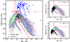 |
Fig. 5. EW(CaT) vs. BP − RP color-coded by density for all selected RVS objects. Overlaid black dots are those with APOGEE measurements of log g. They are plotted separately to represent the positions of different types of stars. The blue dots in the left panel are the known Galactic RSGs mentioned in Sect. 3.1.1. The red asterisks mark the positions of zero-extinction K1 and M2-M5 RSGs. The solid red lines represent the bluest boundary of Galactic RSGs in this diagram, while the dashed red line marks the dividing line between the early- and late-type RSGs. |
With the results from Sects. 3.1.1 and 3.1.2, the bluest boundary of the Galactic RSGs is delineated in Fig. 5 by the solid red line. The upper lines are determined by the (BP − RP)0 = 1.548 for K1-type RSGs and an EW(CaT) value of 1.1 nm before M2. For M2 to M5 types, a linear fitting between EW(CaT) and (BP − RP)0 is used to describe the approximate bluest boundary of RSGs in the EW(CaT) versus BP − RP diagram. Since the Teff and (BP − RP)0 for RSGs later than M5 are unknown, a roughly parallel line to the right branch of the RVS sources is manually drawn to indicate the boundary for later-type RSGs. The known Galactic RSGs (as described in Sect. 3.1.1) indicated by blue dots in Fig. 5 are all on the right side of the boundary lines. Moreover, 576 stars with log g < 1 from the APOGEE catalog, which are considered to be candidates of supergiants, are also located in this area. Further inspection reveals that sources located to the left of the boundary line have lower metallicity, indicating that they are unlikely to be young, metal-rich RSGs. Both results demonstrate that the boundary lines are reasonable.
Following the boundary lines, the RSG candidates are distributed in two areas in Fig. 5, which are separated by the dashed red line at EW(CaT) = 1.1 nm. Stars above and below this line are classified as early-type and late-type RSG candidates, respectively. As to the late-type candidates, the EW(CaT) decreases with BP − RP, suggesting these stars are late-M type bright stars. Although the intrinsic color index of RSGs is almost the same as dwarfs or giants, the observed color index is significantly red because high-luminosity RSGs experience much more extinction. Therefore, these objects are on the right branch in Fig. 5, as expected.
3.2. The early-type RSG candidates
As described in Sect. 3.1.3, early-type RSG candidates in our sample are defined as sources with BP − RP > 1.584 and EW(CaT) > 1.1 nm. Out of the remaining 105 652 sources, 30 meet these criteria, which are presented in Table A.1. The relative errors of EW(CaT) of all 30 stars are below 6%, as their EW(CaT) values are sufficiently large, ensuring precise measurements. Gaia DR3 provides stellar spectral types through the column spectraltype_esphs in the astrophysical_parameters table, which includes OBAFGKM and C stars. This classification is primarily based on specific spectral features in BP/RP spectra, such as the dominance of CN and C2 bands in carbon stars, and the presence of TiO and VO in M-type stars (Lebzelter et al. 2023; Messineo 2023). Among the 30 early-type RSG candidates, 24 and 4 are marked as K-type and M-type stars, respectively, which aligns with expectations since these candidates are expected to be late-K or early-M types. One source is marked as a C star (source_id: 5853442496285943424). However, its BP/RP (XP hereafter) spectrum does not show any significant carbon absorption bands when compared with the XP spectra library of C-rich star of Messineo (2023), suggesting this is likely a misclassification by Gaia. Another source is marked as an O-type star (source_id: 5546711192039738752), but its XP spectrum is not blue-peaked, while with clear TiO absorption features, indicating this is a late-type M star.
Regarding stellar parameters, five stars in the sample have available Apsis GSP-phot parameters, which are derived by fitting XP spectra using PHOENIX or MARCS models to provide best-fit estimates of Teff, log g, and [Fe/H] (Andrae et al. 2023; Fouesneau et al. 2023). Their Teff values are 4451 K, 4455 K, 4524 K, 4568 K, and 5123 K, with log g values between 0.87 and 1.58, consistent with early-type RSG characteristics. However, as described in Fouesneau et al. (2023), the logposterior_gspphot column indicates the quality of the Apsis GSP-phot fitting, with higher values for better fittings. It is recommended to only use results with logposterior_gspphot > −1000. Unfortunately, the highest value among these five stars is −9000. As Messineo (2023) pointed out, the Gaia Apsis pipeline struggles to handle bright late-type stars due to their significant variability and fitting challenges, suggesting that these parameters may not be highly reliable and should be treated cautiously.
Additionally, 28 stars in the sample have Apsis GSP-spec parameters, which are derived from RVS spectra (Recio-Blanco et al. 2023). Following recommendations from Recio-Blanco et al. (2023) and Messineo (2023), sources are filtered by requiring the first nine digits of flags_gspspec to be less than or equal to 1, and the 10th–12th digits to be non-null. Moreover, Recio-Blanco et al. (2023) indicated that due to parameterization issues in GSP-Spec, cool stars with Teff ≲ 4000 K had their parameters set to Teff = 4250 ± 500 K and log g = 1.5 ± 1. After accounting for these limitations, eight stars remain with reliable parameters. Their Teff ranges from 3782 K to 4632 K, and log g values span from −0.29 to 0.65, which are also consistent with typical RSGs.
In summary, the stellar parameters derived from the Gaia Apsis pipeline coincide with RSGs for the 30 early-type candidates despite the high uncertainty.
3.3. The late-type RSG candidates
3.3.1. TiO band
As described in Sect. 3.1.3, late-type RSGs can only be distributed along the right branch of Fig. 5, where EW(CaT) < 1.1 nm, and on the right side of the solid red line. This subset contains 20 873 stars. Because late-type RSGs are cool, oxygen-rich stars, their spectra should feature strong TiO bands. Typically, TiO absorption starts to appear in M2-type stars, peaks at M6, and then saturates. Prominent TiO bands in RSGs include those at 8432+8442+8452 Å and 8859 Å, unfortunately, none of these are covered by the RVS spectra. On the other hand, the XP spectra covers a wide wavelength range, including several strong TiO bands, which are used to screen oxygen-rich M-type stars.
Messineo (2023) identified five TiO absorption features in their XP spectral library, centered approximately at 670, 715, 770, 850, and 940 nm. Given that the 940 nm region also includes absorption from ZrO and CN, only the first four bands are used. Specifically, four wavelength ranges are examined, namely 654–698 nm, 698–750 nm, 750–818 nm, and 818–880 nm. If a single local minimum is detected within any of these ranges, TiO absorption is considered present, and its equivalent width is measured. The equivalent width is calculated by linearly fitting the endpoints of each range to represent a pseudo-continuum, following the method described in Sect. 2.2.2. This approach is reasonable because the endpoints for each range are chosen at the flux maxima of true M-type oxygen-rich stars, and the region between two adjacent flux peaks is designated as the TiO absorption band as shown in Fig. 6. This also minimizes the potential contamination by C or S-type stars, as their dominant molecular bands and flux minima are located at different wavelengths, producing distinctly different spectral shapes (Lebzelter et al. 2023). It can be seen in Fig. 6 that the spectral shape of C star and S-type star is quite different from oxygen-rich star, making the classification reliable. For insurance, only sources that exhibit TiO absorption in at least two of the four bands are considered true M-type oxygen-rich stars. The equivalent widths of all detectable TiO bands are averaged to yield a single EW(TiO) value. Consequently, 1480 stars are excluded from the sample, 848 of which are excluded due to the lack of XP spectra.
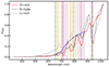 |
Fig. 6. Examples of three XP spectra of an oxygen-rich star (source_id: 5853243278519978112, solid red line), a carbon-rich star (source_id: 5716487091710504064, dashed gray line), and an S-type star (source_id: 5233074194539855360, dashed black line). The spectra are normalized to the maximum flux for comparison. The shaded color denotes the ranges of the four measured TiO bands. The four solid blue lines represent the pseudo-continuum of measuring equivalent width. |
Figure 7 shows the distribution of EW(TiO) in the right branch of EW(CaT) versus BP − RP diagram. It reveals that smaller and larger EW(TiO) values correspond to bluer and redder sources, respectively. Since TiO is a reliable indicator of spectral type, the descending branch on the right side of Fig. 7 corresponds to an increase in spectral type. This is further supported by the relation between EW(TiO) and Teff from APOGEE measurements, as shown in the left panel of Fig. 8. A comparison between EW(TiO) and log g from APOGEE is also presented in the right panel of Fig. 8, which shows that higher EW(TiO) values correspond to lower log g, and vice versa, consistent with the conclusions of Negueruela et al. (2011, see their Fig. 3). The GSP-phot parameters are used to check the relation because they are available for many more sources, although with relatively large uncertainty. As shown in gray dots in Fig. 8, this trend is confirmed.
 |
Fig. 7. Same as Fig. 5, but the regions for late-type RSG candidates are color-coded by EW(TiO) and the rest are shown as gray dots. |
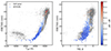 |
Fig. 8. Relation of EW(TiO) with Teff and log g. The dots color-coded by BP − RP are APOGEE measurements, while the gray dots are from Gaia GSP-phot parameters. There are 655 and 5934 stars with available APOGEE and GSP-phot parameters, respectively. |
The remaining 20 873 stars by this step include late-type red giant branch (RGB), RSG, and asymptotic giant branch (AGB) stars. There are two reasons to believe that the blue dots in Fig. 7 likely represent late-type RGB stars (i.e., stars close to the tip of the RGB). First, Dixon et al. (2023) identified metal-poor tip-RGB stars at high Galactic latitudes, with BP − RP ranging from 1.55 to 2.25. For sources with higher metallicity or lower Galactic latitudes, the color would be redder, which aligns with the stars with BP − RP < 3 (blue dots in Fig. 7). Second, these blue points generally exhibit EW(TiO) values below 5–10 nm, which correspond to sources with log g > 1 in Fig. 8, a characteristic of bright giants. Additionally, Fig. 9 shows a bimodal distribution of EW(TiO), further indicating the presence of two distinct stellar populations. To minimize contamination from late-type red giants, only sources with EW(TiO) > 10 nm are selected, leaving 13 316 stars.
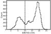 |
Fig. 9. Histogram of EW(TiO). The vertical black line marks the position where EW(TiO) = 10 nm. |
3.3.2. VO band
Both TiO and VO are excellent temperature indicators. After TiO, VO only starts to appear in extremely late-type stars, beginning with M6-type (Kirkpatrick et al. 1991; MacConnell et al. 1992). In Sect. 3.3.1, it is mentioned that the descending branch on the right side of Fig. 5 should indicate an increase in spectral type. To further support this point, the only VO band within the RVS spectral range at 8624 Å in air, (Dorda et al. 2016) is measured.
For this VO band, following the analysis of Dorda et al. (2016), its equivalent width is measured within the range 8624.25–8625.5 Å in air, corresponding to 862.66–862.79 nm in vacuum, and the value is denoted as EW(VO). Figure 10 presents the relation between EW(VO) and EW(TiO), showing all the sources with TiO absorption (i.e., including the sources excluded in Sect. 3.3.1 with EW(TiO) < 10 nm). The intensity of the TiO band increases with spectral type (i.e., as temperature decreases), which manifests as a vertical branch on the left side of the figure. TiO absorption saturates around M6, at which point VO begins to appear and strengthens, forming a horizontal branch on the right side. It is evident that the horizontal branch corresponds to redder sources indicated by a large BP − RP, which aligns with the far-right region in Fig. 5. This suggests that the latest-type stars are located in this region. However, since the red wing of the diffuse interstellar band near 8621 Å may invade the VO band (Zhao et al. 2021; Gaia Collaboration 2023a; Zhao et al. 2024), and this VO band is so weak that it is difficult to measure at low S/N, this analysis is only presented for demonstration and is not used as a selection criterion.
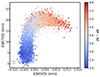 |
Fig. 10. EW(TiO) vs. EW(VO) diagram for all sources exhibiting TiO absorption. The dots are color-coded by BP − RP. |
3.3.3. Removal of AGB stars
At this point, the only potential contamination in the sample comes from AGB stars. Given that AGB stars are generally long-period variables (LPVs) with more significant mass loss and larger variation amplitudes than RSGs, the diagram of K − W3 versus BP amplitude and period–amplitude sequence are used to exclude mass-losing AGB stars and low mass-loss AGB stars, respectively.
The K and W3 magnitudes are taken from the Two Micron All Sky Survey (2MASS; Skrutskie et al. 2006) and the AllWISE catalog from Wide-field Infrared Survey Explorer mission (Cutri et al. 2013), respectively. The BP amplitude is defined by Belokurov et al. (2017) as

All the remaining sources are shown in Fig. 11 (left panel), together with the Galactic AGB stars identified by Suh (2021) using the Infrared Astronomical Satellite (IRAS) data (right panel). Considering the color index K − W3 is a well-known indicator sensitive to dust emission (Xue et al. 2016), and the AGB stars from Suh (2021) mostly have K − W3 > 0.5, such sources in our sample are identified as AGB stars and removed. This criterion is reinforced by the fact that the excluded sources also exhibit larger amplitudes. This process removed 6533 stars from our sample. It is important to note that ∼1400 stars in the K band and ∼100 stars in the W3 band in the sample have poor photometric quality, with their flags not marked with an “A” in the catalog. Further examination reveals that these sources are the brightest stars in the sample, with nearly all having K-band magnitude < 4.5 and W3-band magnitude < 0.5, respectively. Given that such bright stars are more likely to be RSGs, no restriction is applied to the photometric quality for this subset. Instead, only stars with K − W3 > 0.5 are excluded, as they are more likely to be AGB stars.
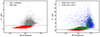 |
Fig. 11. K − W3 vs. BP amplitude diagram for stars that have EW(TiO) > 10 nm. The BP amplitude is defined by Eq. (2). The red dots in both panels are selected late-type RSG candidates, while the gray dots are stars considered to be AGB stars. The blue and green dots in the right panel are the oxygen-rich AGB (OAGB) and carbon-rich AGB (CAGB) stars identified by Suh (2021), respectively. |
Low mass-loss AGB stars can be identified by examining their period–amplitude sequences, for which the LPV catalog in Gaia DR3 (Lebzelter et al. 2023) provides an excellent opportunity. Observations of the LMC have confirmed that LPVs build at least five sequences on the period–luminosity diagram (PLD): A, B, C’, C, and D (see, e.g., Wood et al. 1999). Sequences A and B have been further divided into several sub-sequences to characterize small-amplitude red giant variables (Soszyński et al. 2007). The PLD is a powerful tool for tracing the evolution of LPVs, as different sequences are often associated with varying metallicity and mass-loss rates (Riebel et al. 2012). McDonald & Trabucchi (2019) studied the characteristics of mass-loss rates on the period–amplitude sequences, finding that sequences A and B typically consist of AGB stars with small amplitudes and low mass-loss rates (less than 10−9 M⊙ yr−1). On the other hand, Jiang et al. (2024) demonstrated that RSGs tend to fall on sequences a2 and C in the PLD. Given the well-studied PLD of the LMC, the RSGs in the LMC can be used to mark a reference region on the period–amplitude diagram, with sequences to the left of the region likely corresponding to low mass-loss AGB stars. By cross-matching the remaining sample with the Gaia DR3 LPV catalog (Lebzelter et al. 2023), there are 1,180 stars with available amplitude and period. Their distributions on the period–amplitude diagram are shown as black points in Fig. 12. For comparison, 235 LMC RSGs from the Ren et al. (2021b) sample, cross-matched with the Gaia DR3 LPV catalog, are displayed as red dots. As shown in Fig. 12, the black dots divide into two branches corresponding to shorter and longer periods, while RSGs generally exhibit periods longer than 100 days. This make sense because RSGs with pulsation periods shorter than 100 days are rarely detected (Ren et al. 2019; Chatys et al. 2019). RSGs with timescales shorter than 100 days usually exhibit irregular variation (Ren & Jiang 2020; Zhang et al. 2024), making it challenging to detect in Gaia’s long-cadence light curves. Consequently, the shorter-period branch in Fig. 12 likely consists of low mass-loss AGB stars. Based on the reference region for RSGs, we manually drew the blue line shown in Fig. 12 and excluded stars to the left of it from our sample. This process results in a final sample of 6196 late-type Galactic RSG candidates from Gaia RVS spectra, as listed in Table A.2.
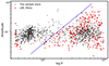 |
Fig. 12. Period–amplitude diagram of our sample stars (black dots) and the LMC RSGs from Ren et al. (2021b, red dots). The amplitude and period are taken from the Gaia DR3 LPV catalog (Lebzelter et al. 2023). The solid blue lines are manually drawn to separate the AGB star branch (short period) and the RSG candidate branch (long period). |
For these late-type RSG candidates, the σ(EW(CaT)) of ∼99.4% sources are lower than 0.07 nm, while ∼99.6% sources have σ(EW(CaT))/EW(CaT) below 20%, further demonstrating the reliability of the measurements. In Gaia’s spectraltype_esphs classifications, all 6196 stars are labeled as M-type, which is encouraging since the sample is indeed expected to contain only O-rich M-type stars. Again, due to the limitations in Gaia Apsis pipeline of bright late-type stars (Messineo 2023), nearly all of the ∼1900 stars with available GSP-phot parameters have logposterior_gspphot values below −1000, indicating that their GSP-phot parameters may be unreliable. Nevertheless, the majority of teff_gspphot values fall between 3200 and 3800 K (∼99%), and logg_gspphot values range from -0.4 to 0.9 (∼99%), which are consistent with the expected characteristics of RSGs. Among the 72 stars with APOGEE measurements, their Teff and log g range from 3300 to 3800 K and 0.1–1.2, respectively, further confirming the robustness of the selection criteria.
4. Discussion
4.1. The known RSGs
Among the 185 known Galactic RSGs mentioned in Sect. 3.1.1, 14 have RVS spectra with S/N > 100, and four of them are identified as late-type RSGs in our analysis. Of the remaining stars, two lack W3-band photometry, while eight have K − W3 color > 0.5. In addition, a cross-match with the RSGs identified by Messineo & Brown (2019) yield 23 stars, 15 of which are absent in the 185 known RSGs. Among these 15 stars, one of them lies to the left of the blue boundary in Fig. 5, and another has the XP spectra characteristics of S-type stars, both of which Messineo & Brown (2019) classified into the F-region, suggesting they are unlikely to be RSGs. Ten of the remaining stars have K − W3 > 0.5, leaving three confirmed as late-type RSG candidates in our sample. The RSGs retained and removed in this work are shown in Fig. 13 as purple (22) and blue crosses (7), respectively. None of the sources listed in other well-known Galactic RSG catalogs are present in the initial sample of this study (i.e., there is no RVS spectrum with a S/N > 100 in Gaia DR3).
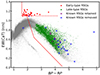 |
Fig. 13. Distribution of RSG candidates selected in this work in the EW(CaT) vs. BP − RP diagram. The red and green dots are the early-type and late-type candidates, respectively. The purple and blue crosses are known RSGs that were retained and removed in this work, respectively. |
4.2. Completeness and pureness
This study identified 30 early-type and 6196 late-type RSG candidates, respectively. Their distribution in the EW(CaT) versus BP − RP diagram is shown in Fig. 13. For early-type RSG candidates, the criteria of BP − RP > 1.584 and EW(CaT) > 1.1 nm ensure a sufficiently complete sample from the released RVS spectra, as these are fundamental characteristics of RSGs. However, potential contamination may arise from yellow supergiants, which share similar EW(CaT) values and slightly bluer BP − RP. If subject to significant extinction, these yellow supergiants could fall within our selection. Another influencing factor is the uncertainty in the EW(CaT) measurements. Taking into account the 6% relative error described in Sect. 3.2, under the most stringent conditions, only stars with EW(CaT) > 1.166 nm (i.e., 1.1 × 10⁶%) can be identified as early-type RSG candidates, resulting in eight such sources. Under the most lenient conditions, an EW(CaT) > 1.034 nm would be sufficient to consider a star an RSG candidate, leading to 394 sources.
For late-type RSGs, the requirement of EW(TiO) > 10 nm when analyzing the XP spectra excludes a portion of sources near BP − RP ∼ 2.5, as evidenced by the absence of candidates in this region in Fig. 13. Known RSGs from previous studies do occupy this region, as shown by the blue dots in the left panel of Fig. 5, indicating possible incompleteness in our sample. However, as described in Sect. 3.3.1, late-type red giants are present in this area, and EW(TiO) reflects stellar surface gravity, supporting the exclusion of stars with EW(TiO) < 10 nm to avoid contamination from red giants. This decision reflects a balance between pureness and completeness, where pureness takes priority.
In addition, the use of the K − W3 < 0.5 criterion likely results in the exclusion of some high-luminosity RSGs, which also possess abundant circumstellar dust caused by significant mass loss. This is indicated by the lack of sources in the lower right corner of Fig. 13, where such RSGs are expected to reside. The clustering of blue crosses at the red end in Fig. 13 confirms this again, as they are likely late-type high-luminosity RSGs. No constraints on photometric quality are used because sources with poorer photometric quality tend to be brighter, making them more likely to be RSGs. This decision is taken to enhance the completeness of our sample, while it may bring about some AGB stars to contamination. By incorporating additional diagnostics from the mid-infrared or far-infrared, it may be possible to improve the sample’s pureness further. Again, this also ensures a pure and relatively complete sample of late-type RSG candidates.
4.3. Application to a larger sample
By slightly lowering the S/N threshold to S/N > 50, the total number of available RVS spectra increases to ∼330 000. Applying the process described in Sect. 3 to these spectra results in the identification of 48 early-type and 11 491 late-type RSG candidates. Although the initial sample size has tripled, the final number of RSG candidates has only doubled. This is expected, as the S/N is correlated with apparent magnitude, meaning that lower S/N sources are likely fainter or of lower photometric quality. It is worth noting that the released RVS spectra do not provide uniform coverage across the sky (Gaia Collaboration 2023b), with noticeably fewer observations in the Galactic plane. Consequently, many RSGs are missed in our sample. We anticipate that the release of the complete RVS spectra in Gaia DR4 will provide a much more comprehensive perspective for identifying RSGs in the Milky Way.
5. Summary
Red supergiants play a crucial role in processes such as interstellar dust production and massive star evolution, making their identification vitally important. While samples of RSGs in nearby galaxies have been expanding greatly thanks to more precise observational data and more effective methods for excluding foreground sources, the search for RSGs within the Milky Way has been slower. This is partly due to the challenges in applying efficient photometric methods, which are hindered by the difficulties in accurately measuring extinction and distance within our galaxy. Moreover, spectroscopic observations have been too inefficient to yield large samples of RSGs. The release of approximately one million RVS spectra in Gaia DR3 offers new possibilities for the search for Galactic RSGs based on spectral features.
In this study, high-S/N (greater than 100) RVS spectra were selected as the initial sample. Firstly, the early-type stars were excluded by using the hydrogen Paschen 14 line. Then, by combining the intrinsic color BP − RP of RSGs of different spectral types with the EW(CaT), the bluest boundary of Galactic RSGs on the EW(CaT) versus BP − RP diagram could be defined. This allowed for the selection of early-type RSGs with BP − RP > 1.584 and EW(CaT) > 1.1 nm and the removal of dwarf stars and the majority of giants, leaving only late-type stars. The analysis of four TiO bands in the XP spectra helped us identify true O-rich M-type stars, thereby avoiding contamination from C-rich and S-type stars. The equivalent widths of the measured TiO bands were averaged and denoted as EW(TiO). Sources with EW(TiO) < 10 nm were considered late-type RGB stars based on their higher log g and bluer colors. The remaining sources were primarily contaminated by AGB stars; those with high mass-loss and low mass-loss were identified by K − W3 > 0.5 and period-amplitude sequences, respectively, and were excluded. This process yielded a final sample of 30 early-type RSG candidates and 6196 late-type RSG candidates.
Applying this method to the RVS spectra with S/N > 50 resulted in the identification of 48 early-type RSG candidates and 11 491 late-type RSG candidates. However, due to the uncertainties involved in processing low-S/N spectra, these numbers are highly uncertain. This work serves as a preliminary study in anticipation of Gaia DR4, when the release of a larger volume of spectra is expected to have profound implications for the study of Galactic RSGs.
Data availability
Tables A.2 is available at the CDS via anonymous ftp to cdsarc.cds.unistra.fr (130.79.128.5) or via https://cdsarc.cds.unistra.fr/viz-bin/cat/J/A+A/694/A152
Acknowledgments
We would like to thank the anonymous referee for the constructive suggestions that definitely improved this work. We thank Dr. R. Dorda for providing the line measurements of stars in the Perseus arm (Dorda et al. 2018). This work is supported by the National Natural Science Foundation of China (NSFC) through grants Nos. 12133002, 12203025, and 12373048. National Key R&D Program of China No. 2019YFA0405503, CMS-CSST-2021-A09 and Shandong Provincial Natural Science Foundation through project ZR2022QA064. H.Z. acknowledges the support of the National Natural Science Foundation of China (grant No. 12203099) and the Jiangsu Funding Program for Excellent Postdoctoral Talent. This work has also made use of data from the surveys by Gaia, APOGEE, 2MASS and WISE.
References
- Abdurro’uf, Accetta, K., Aerts, C., et al. 2022, ApJS, 259, 35 [NASA ADS] [CrossRef] [Google Scholar]
- Alexander, M. J., Kobulnicky, H. A., Clemens, D. P., et al. 2009, AJ, 137, 4824 [NASA ADS] [CrossRef] [Google Scholar]
- Andrae, R., Fouesneau, M., Sordo, R., et al. 2023, A&A, 674, A27 [CrossRef] [EDP Sciences] [Google Scholar]
- Astropy-Specutils Development Team 2019, Astrophysics Source Code Library [record ascl:1902.012] [Google Scholar]
- Beasor, E. R., Davies, B., Smith, N., et al. 2020, MNRAS, 492, 5994 [Google Scholar]
- Belokurov, V., Erkal, D., Deason, A. J., et al. 2017, MNRAS, 466, 4711 [Google Scholar]
- Carquillat, M. J., Jaschek, C., Jaschek, M., & Ginestet, N. 1997, A&AS, 123, 5 [NASA ADS] [CrossRef] [EDP Sciences] [Google Scholar]
- Cenarro, A. J., Cardiel, N., Gorgas, J., et al. 2001a, MNRAS, 326, 959 [NASA ADS] [CrossRef] [Google Scholar]
- Cenarro, A. J., Gorgas, J., Cardiel, N., et al. 2001b, MNRAS, 326, 981 [NASA ADS] [CrossRef] [Google Scholar]
- Cesetti, M., Pizzella, A., Ivanov, V. D., et al. 2013, A&A, 549, A129 [NASA ADS] [CrossRef] [EDP Sciences] [Google Scholar]
- Chatys, F. W., Bedding, T. R., Murphy, S. J., et al. 2019, MNRAS, 487, 4832 [CrossRef] [Google Scholar]
- Chiavassa, A., Pasquato, E., Jorissen, A., et al. 2011, A&A, 528, A120 [NASA ADS] [CrossRef] [EDP Sciences] [Google Scholar]
- Choi, J., Dotter, A., Conroy, C., et al. 2016, ApJ, 823, 102 [Google Scholar]
- Clark, J. S., Negueruela, I., Davies, B., et al. 2009, A&A, 498, 109 [NASA ADS] [CrossRef] [EDP Sciences] [Google Scholar]
- Contursi, G., de Laverny, P., Recio-Blanco, A., & Palicio, P. A. 2021, A&A, 654, A130 [NASA ADS] [CrossRef] [EDP Sciences] [Google Scholar]
- Creevey, O. L., Sordo, R., Pailler, F., et al. 2023, A&A, 674, A26 [NASA ADS] [CrossRef] [EDP Sciences] [Google Scholar]
- Cropper, M., Katz, D., Sartoretti, P., et al. 2018, A&A, 616, A5 [NASA ADS] [CrossRef] [EDP Sciences] [Google Scholar]
- Cutri, R. M., Wright, E. L., Conrow, T., et al. 2013, VizieR Online Data Catalog: AllWISE Data Release (Cutri+ 2013), VizieR On-line Data Catalog: II/328. Originally published in:IPAC/Caltech (2013) [Google Scholar]
- Davies, B., Figer, D. F., Kudritzki, R.-P., et al. 2007, ApJ, 671, 781 [NASA ADS] [CrossRef] [Google Scholar]
- Davies, B., Figer, D. F., Law, C. J., et al. 2008, ApJ, 676, 1016 [Google Scholar]
- Decin, L., Richards, A. M. S., Marchant, P., & Sana, H. 2024, A&A, 681, A17 [NASA ADS] [CrossRef] [EDP Sciences] [Google Scholar]
- Diaz, A. I., Terlevich, E., & Terlevich, R. 1989, MNRAS, 239, 325 [NASA ADS] [CrossRef] [Google Scholar]
- Dicenzo, B., & Levesque, E. M. 2019, AJ, 157, 167 [NASA ADS] [CrossRef] [Google Scholar]
- Dixon, M., Mould, J., Flynn, C., et al. 2023, MNRAS, 523, 2283 [NASA ADS] [CrossRef] [Google Scholar]
- Dorda, R., González-Fernández, C., & Negueruela, I. 2016, A&A, 595, A105 [NASA ADS] [CrossRef] [EDP Sciences] [Google Scholar]
- Dorda, R., Negueruela, I., & González-Fernández, C. 2018, MNRAS, 475, 2003 [CrossRef] [Google Scholar]
- Dotter, A. 2016, ApJS, 222, 8 [Google Scholar]
- Figer, D. F., MacKenty, J. W., Robberto, M., et al. 2006, ApJ, 643, 1166 [Google Scholar]
- Fouesneau, M., Frémat, Y., Andrae, R., et al. 2023, A&A, 674, A28 [NASA ADS] [CrossRef] [EDP Sciences] [Google Scholar]
- Gaia Collaboration (Prusti, T., et al.) 2016, A&A, 595, A1 [NASA ADS] [CrossRef] [EDP Sciences] [Google Scholar]
- Gaia Collaboration (Schultheis, M., et al.) 2023a, A&A, 674, A40 [CrossRef] [EDP Sciences] [Google Scholar]
- Gaia Collaboration (Vallenari, A., et al.) 2023b, A&A, 674, A1 [NASA ADS] [CrossRef] [EDP Sciences] [Google Scholar]
- Garmany, C. D., & Stencel, R. E. 1992, A&AS, 94, 211 [NASA ADS] [Google Scholar]
- Gehrz, R. 1989, in Interstellar Dust, eds. L. J. Allamandola, & A. G. G. M. Tielens, IAU Symp., 135, 445 [NASA ADS] [CrossRef] [Google Scholar]
- Ginestet, N., Carquillat, J. M., Jaschek, M., & Jaschek, C. 1994, A&AS, 108, 359 [NASA ADS] [Google Scholar]
- Healy, S., Horiuchi, S., Colomer Molla, M., et al. 2024, MNRAS, 529, 3630 [NASA ADS] [CrossRef] [Google Scholar]
- Humphreys, R. M. 1978, ApJS, 38, 309 [NASA ADS] [CrossRef] [Google Scholar]
- Humphreys, R. M., & Davidson, K. 1979, ApJ, 232, 409 [Google Scholar]
- Humphreys, R. M., Pennington, R. L., Jones, T. J., & Ghigo, F. D. 1988, AJ, 96, 1884 [Google Scholar]
- Humphreys, R. M., Helmel, G., Jones, T. J., & Gordon, M. S. 2020, AJ, 160, 145 [NASA ADS] [CrossRef] [Google Scholar]
- Jennings, J., & Levesque, E. M. 2016, ApJ, 821, 131 [NASA ADS] [CrossRef] [Google Scholar]
- Jiang, B., Ren, Y., & Yang, M. 2024, in IAU Symposium, eds. R. de Grijs, P. A. Whitelock, & M. Catelan, 376, 292 [NASA ADS] [Google Scholar]
- Katz, D., Sartoretti, P., Guerrier, A., et al. 2023, A&A, 674, A5 [NASA ADS] [CrossRef] [EDP Sciences] [Google Scholar]
- Kirkpatrick, J. D., Henry, T. J., & McCarthy, D. W., Jr. 1991, ApJS, 77, 417 [Google Scholar]
- Kiss, L. L., Szabó, G. M., & Bedding, T. R. 2006, MNRAS, 372, 1721 [Google Scholar]
- Lebzelter, T., Mowlavi, N., Lecoeur-Taibi, I., et al. 2023, A&A, 674, A15 [NASA ADS] [CrossRef] [EDP Sciences] [Google Scholar]
- Levesque, E. M., & Massey, P. 2012, AJ, 144, 2 [CrossRef] [Google Scholar]
- Levesque, E. M., Massey, P., Olsen, K. A. G., et al. 2005, ApJ, 628, 973 [Google Scholar]
- MacConnell, D. J., Wing, R. F., & Costa, E. 1992, AJ, 104, 821 [Google Scholar]
- Mallik, S. V. 1994, A&AS, 103, 279 [NASA ADS] [Google Scholar]
- Mallik, S. V. 1997, A&AS, 124, 359 [NASA ADS] [CrossRef] [EDP Sciences] [Google Scholar]
- Massey, P. 1998, ApJ, 501, 153 [Google Scholar]
- Massey, P., & Olsen, K. A. G. 2003, AJ, 126, 2867 [NASA ADS] [CrossRef] [Google Scholar]
- McDonald, I., & Trabucchi, M. 2019, MNRAS, 484, 4678 [Google Scholar]
- Messineo, M. 2023, A&A, 671, A148 [NASA ADS] [CrossRef] [EDP Sciences] [Google Scholar]
- Messineo, M., & Brown, A. G. A. 2019, AJ, 158, 20 [NASA ADS] [CrossRef] [Google Scholar]
- Nakamura, K., Horiuchi, S., Tanaka, M., et al. 2016, MNRAS, 461, 3296 [NASA ADS] [CrossRef] [Google Scholar]
- Negueruela, I., González-Fernández, C., Marco, A., Clark, J. S., & Martínez-Núñez, S. 2010, A&A, 513, A74 [NASA ADS] [CrossRef] [EDP Sciences] [Google Scholar]
- Negueruela, I., González-Fernández, C., Marco, A., & Clark, J. S. 2011, A&A, 528, A59 [NASA ADS] [CrossRef] [EDP Sciences] [Google Scholar]
- Negueruela, I., Marco, A., González-Fernández, C., et al. 2012, A&A, 547, A15 [NASA ADS] [CrossRef] [EDP Sciences] [Google Scholar]
- Paxton, B., Bildsten, L., Dotter, A., et al. 2011, ApJS, 192, 3 [Google Scholar]
- Paxton, B., Cantiello, M., Arras, P., et al. 2013, ApJS, 208, 4 [Google Scholar]
- Paxton, B., Marchant, P., Schwab, J., et al. 2015, ApJS, 220, 15 [Google Scholar]
- Recio-Blanco, A., de Laverny, P., Palicio, P. A., et al. 2023, A&A, 674, A29 [NASA ADS] [CrossRef] [EDP Sciences] [Google Scholar]
- Ren, Y., & Jiang, B.-W. 2020, ApJ, 898, 24 [NASA ADS] [CrossRef] [Google Scholar]
- Ren, Y., Jiang, B.-W., Yang, M., & Gao, J. 2019, ApJS, 241, 35 [NASA ADS] [CrossRef] [Google Scholar]
- Ren, Y., Jiang, B., Yang, M., et al. 2021a, ApJ, 907, 18 [Google Scholar]
- Ren, Y., Jiang, B., Yang, M., Wang, T., & Ren, T. 2021b, ApJ, 923, 232 [NASA ADS] [CrossRef] [Google Scholar]
- Riebel, D., Srinivasan, S., Sargent, B., & Meixner, M. 2012, ApJ, 753, 71 [NASA ADS] [CrossRef] [Google Scholar]
- Samus’, N. N., Kazarovets, E. V., Durlevich, O. V., Kireeva, N. N., & Pastukhova, E. N. 2017, Astronomy Reports, 61, 80 [CrossRef] [Google Scholar]
- Sartoretti, P., Katz, D., Cropper, M., et al. 2018, A&A, 616, A6 [NASA ADS] [CrossRef] [EDP Sciences] [Google Scholar]
- Sartoretti, P., Marchal, O., Babusiaux, C., et al. 2023, A&A, 674, A6 [NASA ADS] [CrossRef] [EDP Sciences] [Google Scholar]
- Schödel, R., Najarro, F., Muzic, K., & Eckart, A. 2010, A&A, 511, A18 [Google Scholar]
- Skiff, B. A. 2014, VizieR Online Data Catalog: Catalogue ofStellar Spectral Classifications (Skiff, 2009- ), VizieR On-lineData Catalog: B/mk. Originally published in: Lowell Observatory(October 2014) [Google Scholar]
- Skrutskie, M. F., Cutri, R. M., Stiening, R., et al. 2006, AJ, 131, 1163 [NASA ADS] [CrossRef] [Google Scholar]
- Soszyński, I., Dziembowski, W. A., Udalski, A., et al. 2007, Acta Astron., 57, 201 [EDP Sciences] [Google Scholar]
- Suh, K.-W. 2021, ApJS, 256, 43 [NASA ADS] [CrossRef] [Google Scholar]
- Vollmann, K., & Eversberg, T. 2006, Astronomische Nachrichten, 327, 862 [NASA ADS] [CrossRef] [Google Scholar]
- Wang, T., Jiang, B., Ren, Y., Yang, M., & Li, J. 2021, ApJ, 912, 112 [NASA ADS] [CrossRef] [Google Scholar]
- Wen, J., Gao, J., Yang, M., et al. 2024, AJ, 167, 51 [NASA ADS] [CrossRef] [Google Scholar]
- Wood, P. R., Alcock, C., Allsman, R. A., et al. 1999, in Asymptotic Giant Branch Stars, eds. T. Le Bertre, A. Lebre, & C. Waelkens, IAU Symp., 191, 151 [Google Scholar]
- Xue, M., Jiang, B. W., Gao, J., et al. 2016, ApJS, 224, 23 [NASA ADS] [CrossRef] [Google Scholar]
- Yang, M., & Jiang, B. W. 2012, ApJ, 754, 35 [NASA ADS] [CrossRef] [Google Scholar]
- Yang, M., Bonanos, A. Z., Jiang, B.-W., et al. 2019, A&A, 629, A91 [NASA ADS] [CrossRef] [EDP Sciences] [Google Scholar]
- Yang, M., Bonanos, A. Z., Jiang, B., et al. 2023, A&A, 676, A84 [NASA ADS] [CrossRef] [EDP Sciences] [Google Scholar]
- Zhang, Z., Ren, Y., Jiang, B., Soszyński, I., & Jayasinghe, T. 2024, ApJ, 969, 81 [NASA ADS] [CrossRef] [Google Scholar]
- Zhao, H., Schultheis, M., Recio-Blanco, A., et al. 2021, A&A, 645, A14 [NASA ADS] [CrossRef] [EDP Sciences] [Google Scholar]
- Zhao, H., Schultheis, M., Qu, C., & Zwitter, T. 2024, A&A, 683, A199 [NASA ADS] [CrossRef] [EDP Sciences] [Google Scholar]
Appendix A: Additional tables
30 early-type RSG candidates from Gaia RVS spectra
6196 late-type RSG candidates from Gaia RVS spectra
All Tables
All Figures
|
Fig. 1. Example of RVS spectrum re-normalization (source_id: 5836392511305856128). The upper panel shows the original spectrum, and the solid red line is obtained via linear fitting of the red dots. The blue on the bottom panel is the re-normalized spectrum, the histogram on the lower right is a distribution of red dots, and the dashed black line marks the mean of its Gaussian fitting, representing the continuum after re-normalization. The shaded colors are used to represent different absorption lines. |
| In the text | |
|
Fig. 2. Example of the RVS spectrum of a typical early-type star (source_id: 2270570062017774976). The position indicated by the arrow marks the Paschen line series P13-P16 for hydrogen. The gray and green shade mark the measuring ranges of P14 and CaT, respectively. |
| In the text | |
|
Fig. 3. Diagram used to remove early-type stars. The horizontal and vertical axes are EW(P14) and the slope mentioned in Sect. 2.1, respectively. The dashed black box defines the area of early-type stars, and the dots are color-coded by BP − RP. |
| In the text | |
|
Fig. 4. Spectral types vs. EW(CaT) for 185 known Galactic RSGs, with their EW(CaT) measurements from Cesetti et al. (2013), Dorda et al. (2018), and Dicenzo & Levesque (2019). For the only magenta asterisk, the results of Dorda et al. (2018) and Dicenzo & Levesque (2019) are represented after being averaged. The crosses denote the sources measured in this work from the Gaia RVS spectra. The solid black lines mark EW(CaT) = 1.1 nm (for K-type or early M-type RSGs) and the decreasing of EW(CaT) with spectral type (for RSGs later than M2). |
| In the text | |
|
Fig. 5. EW(CaT) vs. BP − RP color-coded by density for all selected RVS objects. Overlaid black dots are those with APOGEE measurements of log g. They are plotted separately to represent the positions of different types of stars. The blue dots in the left panel are the known Galactic RSGs mentioned in Sect. 3.1.1. The red asterisks mark the positions of zero-extinction K1 and M2-M5 RSGs. The solid red lines represent the bluest boundary of Galactic RSGs in this diagram, while the dashed red line marks the dividing line between the early- and late-type RSGs. |
| In the text | |
|
Fig. 6. Examples of three XP spectra of an oxygen-rich star (source_id: 5853243278519978112, solid red line), a carbon-rich star (source_id: 5716487091710504064, dashed gray line), and an S-type star (source_id: 5233074194539855360, dashed black line). The spectra are normalized to the maximum flux for comparison. The shaded color denotes the ranges of the four measured TiO bands. The four solid blue lines represent the pseudo-continuum of measuring equivalent width. |
| In the text | |
|
Fig. 7. Same as Fig. 5, but the regions for late-type RSG candidates are color-coded by EW(TiO) and the rest are shown as gray dots. |
| In the text | |
|
Fig. 8. Relation of EW(TiO) with Teff and log g. The dots color-coded by BP − RP are APOGEE measurements, while the gray dots are from Gaia GSP-phot parameters. There are 655 and 5934 stars with available APOGEE and GSP-phot parameters, respectively. |
| In the text | |
|
Fig. 9. Histogram of EW(TiO). The vertical black line marks the position where EW(TiO) = 10 nm. |
| In the text | |
|
Fig. 10. EW(TiO) vs. EW(VO) diagram for all sources exhibiting TiO absorption. The dots are color-coded by BP − RP. |
| In the text | |
|
Fig. 11. K − W3 vs. BP amplitude diagram for stars that have EW(TiO) > 10 nm. The BP amplitude is defined by Eq. (2). The red dots in both panels are selected late-type RSG candidates, while the gray dots are stars considered to be AGB stars. The blue and green dots in the right panel are the oxygen-rich AGB (OAGB) and carbon-rich AGB (CAGB) stars identified by Suh (2021), respectively. |
| In the text | |
|
Fig. 12. Period–amplitude diagram of our sample stars (black dots) and the LMC RSGs from Ren et al. (2021b, red dots). The amplitude and period are taken from the Gaia DR3 LPV catalog (Lebzelter et al. 2023). The solid blue lines are manually drawn to separate the AGB star branch (short period) and the RSG candidate branch (long period). |
| In the text | |
|
Fig. 13. Distribution of RSG candidates selected in this work in the EW(CaT) vs. BP − RP diagram. The red and green dots are the early-type and late-type candidates, respectively. The purple and blue crosses are known RSGs that were retained and removed in this work, respectively. |
| In the text | |
Current usage metrics show cumulative count of Article Views (full-text article views including HTML views, PDF and ePub downloads, according to the available data) and Abstracts Views on Vision4Press platform.
Data correspond to usage on the plateform after 2015. The current usage metrics is available 48-96 hours after online publication and is updated daily on week days.
Initial download of the metrics may take a while.