| Issue |
A&A
Volume 694, February 2025
|
|
|---|---|---|
| Article Number | A75 | |
| Number of page(s) | 10 | |
| Section | Extragalactic astronomy | |
| DOI | https://doi.org/10.1051/0004-6361/202452221 | |
| Published online | 04 February 2025 | |
Rotation Measure study of FRB 20180916B with the uGMRT
1
Max-Planck-Institute for Radio Astronomy, Auf dem Hügel 69, 53121 Bonn, Germany
2
Department of Astrophysical Sciences, Princeton University, Princeton, NJ 08544, USA
3
National Centre for Radio Astrophysics, Ganeshkhind, Post bag 3 411 007 Pune, India
4
Department of Physics, McGill University, 3600 rue University, Montréal, QC H3A 2T8, Canada
5
Trottier Space Institute, McGill University, 3550 rue University, Montréal, QC H3A 2A7, Canada
6
Jet Propulsion Laboratory, California Institute of Technology, Pasadena, CA 91109, USA
⋆ Corresponding author; This email address is being protected from spambots. You need JavaScript enabled to view it.
Received:
12
September
2024
Accepted:
11
December
2024
Abstract
Context. Fast Radio Burst 20180916B is a repeating FRB whose activity window has a 16.34-day periodicity that also shifts and varies in duration with the observing frequency. Recent observations report that the FRB has started to show an increasing trend in secular Rotation Measure (RM) after only showing stochastic variability around a constant value of −114.6 rad m−2 since its discovery. RM studies let us directly probe the magnetic field structure in the local environment of the FRB. The trend of the variability can be used to constrain progenitor models of the FRB. Hence, further study of the RM variability forms the basis of this work.
Aims. We studied the local environment of FRB 20180916B. We did so by focusing on polarization properties, namely RM, and studied how it varies with time. The data comes from the ongoing campaigns of FRB 20180916B using the upgraded Giant Metrewave Radio Telescope (uGMRT). The majority of the observations are in Band 4, which is centered at 650 MHz with 200 MHz bandwidth. Additionally, we used a few observations where we had simultaneous coverage in Band 4 and Band 5 (centered at 1100 MHz).
Methods. We applied a standard single-pulse search pipeline to search for bursts. In total, we detected 116 bursts with ∼36 hours of on-source time spanning 1200 days from December 2020 to February 2024, with two bursts detected during simultaneous frequency coverage observations. We developed and applied a polarization calibration strategy suited for our dataset. On the calibrated bursts, we used QU-fitting to measure RM. We verified the veracity of calibration solution and RM measurement by performing RM measurements on single pulses of PSR J0139+5814. We also measured various other properties such as rate, linear polarization fraction, and fluence distribution.
Results. Of the 116 detected bursts, we could calibrate 79 of them. We observed in our early observations that the RM continued to follow a secular linear trend, as already seen in past observations. However, our later observations suggest that the source switched from the linear trend to stochastic variations around a constant value of −58.75 rad m−2. It has ceased any secular variability and is only showing stochastic variability. Using the predicted Milky Way RM contribution, we report a tentative detection of a sign flip in the RM in the host galaxy host-frame. We also studied a cumulative rate against fluence and note that the rate at higher fluences (1.2 Jy ms) scales as γ = −1.09(7), whereas that at lower fluences (between 0.2 and 1.2 Jy ms) only scales as γ = −0.51(1), meaning the rate at the higher fluence regime is steeper than at the lower fluence regime. Finally, we qualitatively assess the two extremely large bandwidth bursts that we detected in our simultaneous multi-band observations.
Conclusions. Future measurements of RM variations would help place stronger constraints on the local environment. Moreover, any periodic behavior in the RM measurements would directly test progenitor models. Therefore, we motivate such endeavors.
Key words: instrumentation: interferometers / instrumentation: polarimeters / methods: data analysis / methods: observational / techniques: polarimetric
© The Authors 2025
 Open Access article, published by EDP Sciences, under the terms of the Creative Commons Attribution License (https://creativecommons.org/licenses/by/4.0), which permits unrestricted use, distribution, and reproduction in any medium, provided the original work is properly cited.
This article is published in open access under the Subscribe to Open model.
Open Access funding provided by Max Planck Society.
1. Introduction
Fast Radio Bursts (FRBs) are short timescale (∼1 ms) transient events at radio wavelengths (Lorimer et al. 2007; Petroff et al. 2019, 2022; Bailes 2022). Based on repeatability, there are two classes of FRBs: repeating FRBs (rFRBs) and apparent nonrepeating FRBs (nrFRBs). Detecting multiple bursts from the same source enables detailed and cumulative studies of the FRB. For example, rFRBs have been localized post-discovery by various interferometers, including the European Very Long Baseline Inteferometry Network (EVN; Chatterjee et al. 2017; Marcote et al. 2020; Kirsten et al. 2022; Nimmo et al. 2022b). For selected rFRBs that showed scintillation, detecting multiple bursts at multiple epochs enabled the scintillation screen location to be constrained (Main et al. 2022; Ocker et al. 2022), and even led to modeling the effect of orbital motion of Earth on the scintillation timescales (Main et al. 2023; Wu et al. 2024). Moreover, Kumar et al. (2024) and Nimmo et al. (2024) show how scintillation can place constraints on the location of the FRB emission region. Exhaustive follow-up of rFRBs, even with small telescopes, enables the detection of extremely rare bright events and can help in suggesting a link between rFRBs and nrFRBs on the basis of energy distributions (Kirsten et al. 2024). Similar follow-ups with sensitive instruments facilitates performing large number statistics on bursts from various rFRBs (Li et al. 2021; Jahns et al. 2023; Hewitt et al. 2022; Lanman et al. 2022; Zhou et al. 2022). The repeating nature makes it easy to perform a fine time resolution study of bursts, which can probe the underlying emission mechanism (Day et al. 2020; Nimmo et al. 2021, 2022a; Hewitt et al. 2023; Snelders et al. 2023). Certainly, rFRBs allow us to study the FRB phenomena in a much greater detail, which would help us understand the FRB phenomena. This paper focuses on a singular rFRB source and presents polarimetric results.
FRB 20180916B is a rFRB discovered by the Canadian Hydrogen Intensity Mapping Experiment/Fast Radio Burst (CHIME/FRB) experiment (CHIME/FRB Collaboration 2019). It is unique in that its activity windows are periodic with a 16.34-day period (Chime/Frb Collaboration 2020), and they shift and vary in length with observing frequency (Pleunis et al. 2021; Pastor-Marazuela et al. 2021; Bethapudi et al. 2023). In other words, the source exhibits periodicity and chromaticity. The source was localized to an edge of a spiral galaxy at a redshift of 0.0337 with EVN (Marcote et al. 2020). Tendulkar et al. (2021), using Hubble Space Telescope (HST) observations of the host galaxy, placed constraints on the age of the FRB source to be on the order of 10 Myr. Kaur et al. (2022) performed HI spectroscopy observations using the upgraded Giant Metrewave Radio Telescope (uGMRT); they report the host galaxy to be gas-rich and have a low star formation rate (SFR), suggesting the host galaxy might have undergone a minor merger in the recent past. Future sensitive observations would further illuminate the local environment and provide an additional constraint on possible source models.
Mckinven et al. (2023a, hereafter RM23), using CHIME/FRB, report that the Rotation Measure (RM) of bursts from FRB 20180916B has started to change. The RMs are consistent with a single value from its discovery until around MJD 59243, but since then they have started to exhibit an increasing trend. The trend is further corroborated by LOFAR detections (Gopinath et al. 2024, hereafter AG23). FRB 20180916B is not the only rFRB to exhibit significant RM variability. Mckinven et al. (2023b) report nearly all repeaters exhibit RM variability, which suggests that repeaters exist in dynamic magneto-ionic environments. This variability, which is local to the repeater, can be used to constrain the origins of FRB (see, e.g., Yang et al. 2023), which predicts RM variability for different FRB progenitor scenarios. However, Sherman et al. (2023) suggest that host galaxies of rFRBs have statistically larger magnetic fields than that of the Milky Way; that is, they suggest that the host galaxy ISM contributes significantly to the FRB RM. In such a case, decoupling host galaxy contribution and local environment would be particularly challenging, but nevertheless will be crucial to place limits on local environments.
This paper mainly presents polarization results from the ongoing observing campaign of FRB 20180916B with the upgraded Giant Metrewave Radio Telescope (uGMRT). In Sect. 2 we describe the observations and the search strategy utilized. Then, Sect. 3 covers the polarization calibration, flux scaling, and RM measurements. Finally, the results and discussions are presented in Sect. 4, and our conclusions in Sect. 5.
2. Observations and searches
2.1. Observations
Observations were performed using uGMRT (Swarup 1991; Gupta et al. 2017). It is a radio interferometer situated in Khodad, near Pune, India. It consists of 30 parabolic dishes, 45 meters in size, that can be used to perform imaging-mode and phased array-mode observations. It offers observation capability from 100 MHz to 1.4 GHz broken into five bands. Our observations used Band 4 (550–750 MHz) and Band 5 (1000–1200 MHz). Observations from GMRT Proposal Cycle 39 (from October 2020 to March 2021), Cycle 43 (from October 2022 to April 2023), and Cycle 45 (from October 2023 to April 2024), as well as one observation from Cycle 42 (from April 2022 to October 2022), are presented in this paper. Each cycle has its own observing strategy, chiefly the time resolution and frequency coverage. All observations were primarily done in Band 4. However, for five observations of Cycle-39, the entire GMRT array was split into two sub-arrays, where one sub-array performed observations in Band 4 and the other in Band 5. This way, simultaneous coverage of Bands 4 and 5 was achieved. All observations of Cycles 39, 43, and 45 have a time resolution of 327.68 μs, whereas the Cycle 42 observations only have a time resolution of 168.34 μs. The number of channels in all the observations was fixed to 2048. We note that all observations of Cycle 45 were strongly affected by strong ionospheric activity. The observations of Cycles 43 and 45 used the realtime radio frequency interference (RFI) filtering system of the uGMRT (Buch et al. 2022, 2023).
Each individual scan is listed in Table 1 for Band 4 and Table 2 for Band 5. In all the cycles, we recorded full coherency 16-bit phased array (PA) filterbank and Stokes-I 16-bit intensity array (IA) filterbank (Roy et al. 2018). The PA-beam is generated using voltages from individual antennas which are summed in phase, thus is a coherent beam. Instead, the IA-beam is constructed using total intensities of each antenna. All the observations are scheduled in the active windows as predicted by the periodicity and chromaticity model (Chime/Frb Collaboration 2020; Pleunis et al. 2021; Pastor-Marazuela et al. 2021; Bethapudi et al. 2023).
Band 4 Observations described in this paper (see the auxiliary material for a machine-readable csv file which include actual scan times).
Band 5 Observations described in this paper.
Each observation consists of science scans, which are bracketed by phasing scans of 0217+738 to phase up the signal from all antennas in the array. Unfortunately, our choice of calibrators and pulsars (for verifying the calibration pipeline) has not been consistent throughout the cycles. Altogether, we observed 3C138 (a polarized quasar), 3C48 and 3C468.1 (unpolarized quasars), noise diode scans (NG), and pulsars: PSR B0329+54 and PSR J0139+5814. Additionally, for some of the observations, we have noise diode scans during which we pointed at an empty patch of sky with the noise diode turned ON. We specify the auxiliary sources in the Aux. column of Table 1. When we discuss the various calibration strategies in Sect. 3.1, we used whichever strategy was possible for an observation based on the available source scans.
2.2. Searches
We subtracted the time aligned IA-beam from the PA-beam and created Stokes-I 8 bit filterbank data. Doing so gets rid of all the RFI common in both beams, while leaving untouched the astrophysical signal, which is only dominantly present in the PA-beam. We then applied a standard PRESTO (Ransom 2011) single-pulse search pipeline. Post subtraction, the data was already clean and we did not need to apply an additional RFI mitigation step (Roy et al. 2018). We searched at a dispersion measure (DM) of 348.82 pc cm−3 at the native time resolution. We searched for candidates that are up to 300 samples wide (100 ms). We manually vetted each of the candidates using a diagnostic plot. For each of the manually vetted candidates, we sliced the original 16bit PA-beam data to create a PSRFITS burst archive (Hotan et al. 2004). All the analysis from now on is carried out on these burst archives. The number of bursts we report are listed in Table 1 for Band 4 and Table 2 for Band 5.
We report a total of 116 bursts in Band 4 and seven bursts in Band 5. Out of the 116 Band 4 bursts, we were only able to polarization calibrate 79 of them because we did not schedule auxiliary sources in some observations (see Table 1). Moreover, we also report two simultaneous detections of bursts in Bands 4 and 5. Unfortunately, the Band 4 bursts of the two simultaneous detections could not be calibrated for the same reason as above. We defer polarization calibration of Band 5 bursts to future work.
3. Analysis
Having created PSRFITS burst archive from the PA-beam data, we first employed PAZI (Hotan et al. 2004) to perform extensive RFI cleaning. Then, we selected the burst region with a rectangle such that the visual extent of the entire burst (that is, where the burst is clearly above the background noise) is covered by it. We call this the ON-burst region. The length along time dimension is the width, defined from start of the burst envelope to its end. The length along frequency dimension is the bandwidth of the burst. We then performed polarization calibration and flux scaling as described in Sects. 3.1 and 3.2. Finally, we measured RM and, polarization fractions as described in Sect. 3.3.
3.1. Polarization calibration
uGMRT in Band 4 has a circular basis, which has two hands: Right Circular Polarized (RCP) and Left Circular Polarized (LCP). To calibrate the polarization response of uGMRT, we require a polarized source, such as 3C138 (polarized quasar) or noise diode (NG). 3C48 is unpolarized; however, we can use 3C48 in conjunction with any pulsar, for example PSR B0329+54 or PSR J0139+5814, to perform the calibration. We judiciously choose a calibration strategy based on whichever auxiliary observations are available (see Table 1). Unfortunately, we also have a few observations where no auxiliary source had been observed. We have no way of performing the polarization calibration, and are forced to omit them from the polarization analysis.
SINGLEAXIS is the simplest model for characterizing the polarization response of the system. This model involves GAIN, a scalar gain term that is a multiplicative factor; DGAIN, which accounts for the differential gain between the two hands; and DPHASE, which measures the cross-hand delay, that is, the delay between the RCP and LCP. We model DPHASE(ϕ) as a linear function of observing frequency (in GHz, denoted by fGHz) as ϕ = ψr + πDnsfGHz. The ψr is a constant term which, on a circular basis, is half the position angle of the infalling radiation. Dns is the cross-hand delay in nanoseconds and is also known as cable delay in the literature.
When computing GAIN and DGAIN using quasar scans, we assume that quasars possess no circular polarization (Perley & Butler 2013). In addition, while the quasar flux density is not flat over frequency (Perley & Butler 2017), we assume the quasar flux density to be same throughout the bandwidth of 200 MHz. We make this assumption because throughout the work, we average over the frequency and quote the measurements at one frequency (which is the central frequency of 650 MHz). Since a noise diode is designed to emit constant pure Stokes-U signal across the bandwidth, the assumptions we make above automatically hold true. Then, for all the quasar and noise diode scans, we subtracted OFF (when looking at an empty patch of sky or when the noise diode is turned OFF) from ON (when looking at the quasar or when the noise diode is turned ON) scans and averaged over time to produce Stokes products against frequency. Using this, we measured GAIN and DGAIN algebraically (Britton 2000, see Eq. 14)1.
We used the Bayesian nested sampling code ULTRANEST (Buchner 2021) to fit for Dns and ψr. The position angle-like term is fixed to be in ![Mathematical equation: $ [ \frac{-\pi}{2}, \frac{\pi}{2} ] $](/articles/aa/full_html/2025/02/aa52221-24/aa52221-24-eq1.gif) . The Dns is restricted to be in [ − 400, 400] ns. We note that the sign of the delay is not a consequence for calibration or RM measurements. We model
. The Dns is restricted to be in [ − 400, 400] ns. We note that the sign of the delay is not a consequence for calibration or RM measurements. We model
![Mathematical equation: $$ \begin{aligned} Q + jU = L_p\ I_{\rm smooth}\ \mathrm{exp} \big [ 1j \big ( \psi _{\rm r} + \pi \mathrm{D}_{\rm ns}f_{\rm GHz} \big ) \big ], \end{aligned} $$](/articles/aa/full_html/2025/02/aa52221-24/aa52221-24-eq2.gif) (1)
(1)
where Lp is the linear polarized fraction, and Ismooth is the Gaussian-smoothed Stokes-I profile over frequency. We used a standard Gaussian likelihood between observed data (Stokes-Q and Stokes-U against frequency) and the model predicted Stokes-Q and -U. Additionally, we treat standard deviation of the OFF scan to be the respective errors in Stokes-Q and -U, and use them in the likelihood. Measuring the cross-hand delay with noise diode scans is straightforward. However, measuring the same using either the 3C138 quasar or pulsars requires a preceding step.
While 3C138 is generally accepted to have zero RM (Perley & Butler 2013), Cotton et al. (1997) suggests the RM to be −2.1 rad m−2. Since we are operating at lower frequencies (compared to L-band and above where VLA operates) where the rotation is more enhanced, we have to take this Faraday rotation into account. In addition, there is also the ionospheric RM contribution, which also inadvertently causes Faraday rotation. The Faraday rotation affects the measurement of the cross-hand delay (ϕ) as both are degenerate. Then, if we incorrectly compensate for cross-hand delay and apply this solution to the bursts, we end up with incorrect RM measurements. Therefore, prior to fitting for ϕ, we de-rotated Stokes-Q and Stokes-U accordingly; that is, we compensated for the spurious RM along the line of sight.
We also measured cross-hand delay using two pulsars, PSR B0329+54 and PSR J0139+5814. Since the pulsars have position angles varying with phase, we do not average over the entire ON-region; instead, we picked just one phase bin which has the highest intensity. We made use of this slice to compute cross-hand delay. As done in the case of 3C138, we also corrected for the literature value of Rotation Measure and ionospheric RM along the line of sight. We estimate the ionospheric RM contribution using Mevius (2018).
3.2. Flux calibration
Flux calibration is performed using the quasar scans. Perley & Butler (2017) is used to estimate the flux scaling which is then applied to the bursts. We note that the flux scaling does not depend on the polarization dimensions, and only affects the scalar GAIN term. Therefore, we can perform flux scaling even for those observations for which we could not perform polarization calibration.
When the calibration is done using quasars (either polarized or unpolarized), the flux calibration is straightforward. When the calibration is done using noise-diode scans, the GAIN term is determined by the noise-diode whose strength is unknown. To circumvent this, we first applied the noise-diode derived calibration solution to the 3C48 quasar scan and then determine the flux scaling from the calibrated 3C48 quasar scan. To those bursts that cannot be polarization calibrated, flux scaling can still be performed because only a known flux source is needed. Having performed flux scaling to all the bursts, we measured the flux and fluence. We first collapsed the frequency axis by averaging over it. Then, we summed over the ON-region to compute the fluence in units of Jy ms. The maximum in the ON-region is the peak flux in mJy. We note that after flux calibration, the OFF-region statistics should be zero mean already, and therefore we do not have to do any OFF-region subtraction here. We tabulate the measurements in Table 3. We assume a 10% error in our flux and fluence measurements as per Nayana & Chandra (2021). For the observations of MJD 60303, MJD 60336 and MJD 60352 (GMRT cycle 45), we could not perform flux calibration because of the heightened ionospheric activity adversely affecting our observations.
Properties of the Band 4 bursts detected in this work.
3.3. RM and polarization fraction measurements
Faraday rotation introduces sinusoidal variations in Stokes-Q,-U as a function of λ2, where λ is the wavelength. We employ the method of QU-fitting to measure RM where we directly fit sinusoidals to Stokes-Q,-U as a function of λ2. We model Stokes-Q,-U as a function of wavelength as
![Mathematical equation: $$ \begin{aligned} Q + jU = L_p\ I_{\rm smooth}\ \mathrm{exp} \big [ 2j \big ( \mathrm{RM} (\lambda ^2 - \lambda _c^2) + \psi \big ) \big ], \end{aligned} $$](/articles/aa/full_html/2025/02/aa52221-24/aa52221-24-eq3.gif) (2)
(2)
where Lp is the linear polarization fraction, ψ is the position angle, Ismooth is the Gaussian smoothened Stokes-I profile as a function of frequency, and λc is the wavelength at the center of the burst frequency envelope. We perform the centering to assist in convergence of the fit. Without doing so, we noted a correlation between RM and ψ in our posterior sampling.
We sampled from the posterior using the nested sampling code ULTRANEST (Buchner 2021). We use a standard Gaussian likelihood function with errors in Stokes-Q and -U, and assume flat priors for all the parameters. Our prior on RM ranges from −400 rad m−2 to 400 rad m−2, and on Lp from 0 to 1. The prior on ψ is in ![Mathematical equation: $ [-\frac{\pi}{2},\frac{\pi}{2}] $](/articles/aa/full_html/2025/02/aa52221-24/aa52221-24-eq4.gif) . The nested sampling algorithm samples from the posterior distribution directly. We take the median and standard deviation of each of the parameters as the measured value and corresponding error. For every burst, we time-averaged the ON-burst and OFF-burst regions in all Stokes channels. Then, we subtracted OFF-burst from ON-burst and used the ON-OFF Stokes-parameters (which are a function of wavelength) for further analysis. We estimated the errors as the standard deviation of the OFF-burst regions. We find that the errors might be underestimated this way, and furthermore any error in calibration can also introduce systematics in the error that otherwise would be left unaccounted for. Therefore, we introduced EQUAD to the QU-fitting to artificially inflate the errors of Stokes-Q, -U. EQUAD is an additional parameter that is fitted for while measuring RM. The prior of EQUAD is also flat and is set to be in [0.,10.]. In the case that the posterior samples of EQUAD were converging to the boundary values, we re-ran the fitting after suitably increasing the EQUAD range. For each fitting, we produced and visually inspected diagnostic plots.
. The nested sampling algorithm samples from the posterior distribution directly. We take the median and standard deviation of each of the parameters as the measured value and corresponding error. For every burst, we time-averaged the ON-burst and OFF-burst regions in all Stokes channels. Then, we subtracted OFF-burst from ON-burst and used the ON-OFF Stokes-parameters (which are a function of wavelength) for further analysis. We estimated the errors as the standard deviation of the OFF-burst regions. We find that the errors might be underestimated this way, and furthermore any error in calibration can also introduce systematics in the error that otherwise would be left unaccounted for. Therefore, we introduced EQUAD to the QU-fitting to artificially inflate the errors of Stokes-Q, -U. EQUAD is an additional parameter that is fitted for while measuring RM. The prior of EQUAD is also flat and is set to be in [0.,10.]. In the case that the posterior samples of EQUAD were converging to the boundary values, we re-ran the fitting after suitably increasing the EQUAD range. For each fitting, we produced and visually inspected diagnostic plots.
The measured RMs and corresponding errors are listed in Table 3. Lastly, we verified our RM measurements in Appendix A.1, and we comment about the DPHASE variability and its affect on RM measurement in Appendix B.
3.3.1. Band 5
uGMRT Band 5 data is on a linear basis. We did not perform any calibration in Band 5 because of a lack of good quality calibrator data. Moreover, since we only have two bright bursts in Band 5, we leave the calibration work to future work. Fortunately, because of linear feeds, it is still possible to measure RM without calibration.
RM measurements are done as already mentioned above using ULTRANEST. The only difference is the addition of a Delay parameter. Starting with a pure linear polarized signal (in this formalism with Stokes-Q), the first transformation undergone by the infalling radiation is the Faraday rotation (parameterized by θ). Then the cross-hand delay is realized, which is parameterized by ϕ. These transformations are computed at every frequency channel with θ = PA + RM(λ2 − λc2) and ϕ = fGHz * π * Dns, Dns denotes the cross-hand delay in nanoseconds:
 (3)
(3)
As done with Band 4 RM measurements, we also included EQUAD to expand errors since we are not actually calibrating the bursts.
It should be noted that our assumption of pure Stokes-Q signal need not be the case. Our input (right-most vector) can be a mixed state, but it can be always be written as a rotation matrix applied to be a pure state. Such a rotation matrix would be a constant and can be absorbed into the right-most matrix. Given that in such a case recovering the position angle would not be straightforward, but since we are not measuring position angles, we are tempted to follow this procedure for the sake of simplicity. We applied this method to only two of the high S/N bursts. The measured RM and their uncertainties are mentioned in Sect. 4.2. We make note of the large errors, and attribute them to an inadequate bandwidth of only 200 MHz while measuring at high frequencies.
Prior to measuring the linear polarization fractions of the bursts, we first corrected each burst with the RM measured from it using PAM (Hotan et al. 2004). Then, we followed the procedure of Everett & Weisberg (2001) to de-bias and measure the linear polarization fractions of the bursts. This has already been specified in great detail (see Nimmo et al. 2021; Bethapudi et al. 2023; Gopinath et al. 2024), and hence is omitted here.
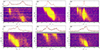 |
Fig. 1. Selection of polarization calibrated bursts. For each burst, we plot the de-dispersed dynamic spectra, frequency averaged total intensity (black) and RM corrected linear polarized (red) time series. The gray bands are RFI channels that have been zapped. The top left text in the time series panels is the burst ID. The rest of the plots can be found on zenodo. |
4. Results and discussions
4.1. Properties
We report a total of 116 bursts collected over 36.50 hours, with which we report a total rate of 3.1 ± 0.5 h−1. The error is 95% Poissonian error. Moreover, we computed the rate from each observing session as well as the total rate and plot it in Fig. 2 (top panel). We also computed the rate and total exposure as a function of activity phase taking into account all the observations (bottom panel). We used the latest measured period of Sand et al. (2023) to compute the phases of the bursts. Moreover, Sand et al. (2023) also report the period derivative, which is consistent with zero, implying that the computed phases of the bursts are valid even for a large time span of data, such as our dataset. Each observation is binned in phase-axis where every phase bin width is 0.03125 (12.25 hours). In the case when any bin was partially overlapped, we added a fractional weight proportional to the overlap. Thereafter, the exposure and number of bursts per each phase bin was computed, which gives rate as a function of phase. We denote the phase bins where we did not detect any bursts with green triangles. We do not see any rate variability over phase. Pastor-Marazuela et al. (2021) modeled rate as a function of phase using kernel density estimates. We cannot yet perform such an analysis because of insufficient sampling of the phase region. Quantitatively, our total observations compose of 36.5 hours, whereas the active window at 600 MHz is about 50 hours (Pleunis et al. 2021; Bethapudi et al. 2023). Therefore, we suggest we would need at least 100 hours of on-source time in total before we can confidently measure phase variability (Sand et al. 2023).
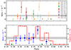 |
Fig. 2. Rate over activity phase of FRB 20180916B. The horizontal dotted black line is the total average rate. The error bars and the shaded region around the horizontal dotted line correspond to 95% error. Top: Rate per phase for each observation color-coded by activity cycle of the source. Detections are marked by diamonds with 95% error bars. Nondetections are marked by triangles. Bottom: Rate over activity phase when all observations are considered (see text for more details). The down-pointing green triangles denote nondetection of bursts. The blue squares correspond to rates with 95% error, with y-axis toward the left. The red circles mark the total exposure at the corresponding phase with y-axis toward the right. |
We investigated the cumulative rate distribution against fluence for our burst sample. Figure 3 shows the cumulative rate above fluence (F) versus fluence for GMRT-Band 4 burst sample as blue squares. We fit broken power laws, where each power law is of the form Rate(≥F)∝Fγ) to it. For our sample we required two break points, 0.18 Jy ms and 1.10 Jy ms, to fit the data. Between 0.18 Jy ms and 1.10 Jy ms, we compute γ = −0.51 ± 0.01, and beyond 1.10 Jy ms, γ = −1.09 ± 0.07. Of the two breakpoints, we treat the smallest fluence break point as the fluence completeness limit. The fluence completeness for our sample agrees well with what is computed using the radiometer assuming a S/N of 10, a maximum width of 40 ms, and RMS noise of 3.36 mJy2. We then repeated the same exercise with the CHIME/FRB FRB 20180916B burst sample (Chime/Frb Collaboration 2020; Pleunis et al. 2021). We plot the cumulative rate versus fluence in the same Fig. 3, but as red circles. For the CHIME sample we required only one breakpoint at 1.67 Jy ms, and γ was fitted to be −1.34 ± 0.11 above it. We note that the uGMRT fluence completeness is ten times smaller than CHIME/FRB, which obviously suggests that GMRT is a sensitive instrument that complements the shallow but daily observations of CHIME/FRB. Pastor-Marazuela et al. (2021) measure γ to be −1.5 ± 0.2 and −1.4 ± 0.1 at 150 MHz (with LOFAR and above 104 Jy ms) and 1370 MHz (with APERTIF and above 7.8 Jy ms), which suggests the γ measurements across frequencies are consistent up to 2σ. However, if it is so that γ at 600–650 MHz is not as steep as compared to other frequencies, it could mean that GMRT is probing a deeper energy regime that is not performed by other telescopes.
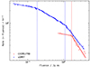 |
Fig. 3. Rate as a function of fluence for CHIME/FRB sample (Chime/Frb Collaboration 2020; Pleunis et al. 2021, in red) and our sample (in blue). Broken powerlaw are fitted to CHIME and our samples. The blue dotted lines are at 0.18 Jy ms and 1.10 Jy ms. The red dotted line is at 1.67 Jy ms. See text for the γ values. |
We do not observe any noticeable DM variations from the inspection of dynamic spectra of the bursts. This observation is strongly corroborated by Sand et al. (2023), which also do not report any DM variation. Additionally, we do not observe any frequency burst envelope variations between regimes when RM was nonvarying and when RM was varying (Mckinven et al. 2023a, cf. Fig. 4). The linear polarization fractions are consistent with measurements of RM23. Linear polarization of the bursts from this FRB undergo depolarization due to scatter in the RM (Feng et al. 2022). The RM scatter is only 0.12 rad m−2, which predicts bursts to be on average 95% linear polarized at our frequency of operation (650 MHz). We note the inverse variance weighted mean linear polarization fraction is 95.0(1)%, which agrees well with the predicted depolarization. Since our linear polarization fraction measurements did not hint at any variability, we did not attempt to fit for RM scatter either on a per observation basis or on the whole. Nevertheless, we encourage the proposition of checking RM scatter variability with time as it could provide a constraint on the temporal variations of RM. We did not measure, and thus, do not report any circular polarization.
4.2. Multi-band bursts
We report two instances where we detected bursts in both of the observing bands (550–750 MHz and 1000–1200 MHz) simultaneously. We plot them in Fig. 4 where we de-disperse both the bands to the same reference frequency of 1200 MHz (top of Band 5). In both the cases we observe the burst is brighter in the upper band that precedes the lower band component. In the case of the multi-frequency burst detected on MJD 59242, the Band 4 component follows the structure of the Band 5 component. Moreover, this burst has a bandwidth of at least 500 MHz and a temporal width of 12 ms. In the multi-frequency burst detected on MJD 59159, the frequency structure fades toward the lower edge of Band 5 and it only reappears from the lower edge of Band 4, implying that the frequency structure is discontinuous. The discontinuity could be at least for 450 MHz, as we do not know if there is a burst component in the missing frequency band from 750 MHz to 1000 MHz. Moreover, the burst structure in Band 4 does not closely match that in Band 5. With only two instances in the entire dataset, we refrain from discussing possible physical scenarios that could cause such bursts. However, we detected two instances with only six hours of observing time, which suggests that these instances are not rare phenomena; therefore, we highly recommend large bandwidth observations of not just FRB 20180916B but also other rFRBs.
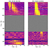 |
Fig. 4. Time-aligned filterbank data of Band 4 (550–750 MHz) and Band 5 (1000–1200 MHz) showing simultaneous detections. The filterbank data has been de-dispersed to 1200 MHz (top of Band 5). The gray region is random data plotted to show continuity. The white strips are manually flagged RFI. The time-frequency resolution and color-scale have been suitable chosen to clearly display the bursts. |
We tried to compare the RMs between the multi-frequency components. For the multi-frequency burst on MJD 59159, the Band 5 RM is −105.38 ± 3.6 rad m−2. For the multi-frequency burst on MJD 59242, the Band 5 RM is −120.4 ± 4.5 rad m−2. We could not measure Band 4 RM because we could not perform polarization calibration. For the MJD 59191 burst, we have no auxiliary scans (see Table 1). For the MJD 59242 burst, our DPHASE solution did not converge, and we could not generate a calibration solution. However, we know that on these MJDs, the RM had not started to change (see the following section). If we assume RM from the epoch when it was not changing (−114.6 rad m−2; Nimmo et al. 2021), the Band 5 RM measurements are within 3σ.
4.3. Band 4 RM
We plot our observed ionospheric corrected RMs against MJDs in Fig. 5 (blue squares). In the same figure, we plot measurements by CHIME/FRB (Mckinven et al. 2023a, red circles) and LOFAR (Pleunis et al. 2021; Gopinath et al. 2024, green diamonds). We highlight the strong consistency between our RM measurements and the CHIME/FRB measurements around MJD 59569. This agreement also musters confidence in our RM measurements. Prior to MJD 59300 the RM is not seen to vary. From MJD 59300 until until MJD 59700, the measurements vary in a linear fashion. RM23 fitted a linear trend to the RM against time with slope of 0.197(6) rad m−2 day−1. This trend is shown with a red broken line in Fig. 5. After MJD 59800, with one LOFAR detection (Gopinath et al. 2024, MJD 59802) and our detections, we see that the RM measurements no longer follow the linear trend of RM23. When seen altogether, we note that RM was exhibiting stochastic variability from MJD 58500 until MJD 59300, then from MJD 59300 to MJD 59700 it exhibited a secular variation, but from MJD 59800 until the end of our measurements at MJD 60352, the RM is seen to vary only stochastically. We also note that as of now, the stochastic variability before and after the linear trend is of the same duration. Future observations would be crucial not only to observe if the increasing trend resumes, but also to see if RM ever goes back to its original value.
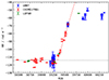 |
Fig. 5. Observed ionosphere corrected RM against MJD. CHIME/FRB RM23 are shown as red circles. LOFAR points are green diamonds AG23. This work’s points are plotted as blue squares. The dotted horizontal line is the reported RM before variability started (Nimmo et al. 2021). The dashed red line is the trend fitted by RM23. |
Mckinven et al. (2023b) shows that most rFRBs exhibit secular RM evolution, often with  . This is also seen in FRB 20180916B. Futhermore, FRB 20180916B is one of the few sources that shows time spans of secular RM variation as well as time spans of no RM variation. Other such sources are PSR J1745-2900 (Eatough et al. 2013), which exhibits RM variability and which parallels FRB 20180916B (Desvignes et al. 2018, see Fig. 3). The RM of PSR J1745-2900 was also seen to vary in a linear fashion (Mckinven et al. 2023a); however, further monitoring shows that the linear trend ceased, but the RM still continued to increase (Gregory Desvignes, priv. comm.). FRB 20121102A (Spitler et al. 2014) has a large absolute RM (∼105) and has exhibited decreasing RM evolution. It also has epochs where the evolution halts (Hilmarsson et al. 2021a; Plavin et al. 2022). There is also FRB 20190520B (Niu et al. 2022), which has an extreme |RM| value and variability. It has already undergone two sign flips within a span of 200 days (Anna-Thomas et al. 2023). FRB 20180301A (Luo et al. 2020), in addition to RM variability with one sign flip, also shows a clear dispersion measure (DM) variability (Kumar et al. 2023). FRB 20201124A (Lanman et al. 2022) showed substantial short-term variability (Hilmarsson et al. 2021b; Xu et al. 2022), but only for a span of 40 days, and became quiescent afterward. On the contrary, FRB 20220912A does not exhibit any RM variability when observed with FAST over s timescale of two months (Zhang et al. 2023).
We investigated if the increasing RM trend shows sign reversal. The Milky Way contribution of RM is estimated to be −98 ± 40 rad m−2 (Hutschenreuter et al. 2022). The largest predicted Milky Way contribution is −58 rad m−2 and the largest ionospheric RM corrected RM measured (on MJD 59993) is −48.8 ± 1.56 rad m−2. There is a tentative detection of sign flip. There are three possible scenarios for observed RM trend: (i) changing electron density, (ii) changing path length of the magnetized Faraday screen, and (iii) changing magnetic field (see also Mckinven et al. 2023b). Changing electron density or path lengths of the active media along the line of sight would cause correlated variations in the DM, which neither RM23 nor Sand et al. (2023) observe; we do not see these variations either. The presence of a sign flip in the RM would strongly suggest that the variations seen are due to changing magnetic fields. Future observations will be extremely crucial in probing if the tentative detection of sign flip is genuine. If that is the case, it would make FRB 20180916B the third FRB, after FRB 20190520B (Anna-Thomas et al. 2023) and FRB 20180301A (Kumar et al. 2023), to show a sign reversal. Lastly, we strongly urge efforts be made to study the large-scale magnetic field structure of the FRB host galaxy. Such a study would provide an alternative line of evidence for the average magnetic field measurements, and would elucidate the role that past mergers (Kaur et al. 2022) may have played in the creation of FRB sources.
There are multiple models involving persistent radio sources (PRSs) at the FRB location that predict RM (and DM) evolution. These models have been proposed for FRB 20121102A, FRB 20190520B, and FRB 20201124A, all of which have PRS detections (Chatterjee et al. 2017; Niu et al. 2022; Bruni et al. 2024). For instance, Piro & Gaensler (2018) postulate that an expanding shocked supernovae remnant (SNR) is the cause of DM and RM evolution. The FRB emitting object is within the SNR and the shocked boundary between the ejecta and background ISM provides the necessary conditions to affect DM and RM with time. Similarly, Margalit & Metzger (2018) propose that the FRB source, a magnetar, is embedded in a magnetized wind nebula (MWNe), which causes the DM and RM variations. Interestingly, Bruni et al. (2024) also attribute RM evolution with PRS, and propose a correlation between luminosity of the PRS and the magnitude of the observed RM. This relation holds for FRB 20121102A and FRB 20190520B, both of which have |RM| in 105 rad m−2 (Hilmarsson et al. 2021a; Anna-Thomas et al. 2023), and also for FRB 20201124A whose |RM| is on the order of 650 rad m−2 (Hilmarsson et al. 2021b; Xu et al. 2022). However, there has only been an upper limit on the luminosity of FRB 20180916B Marcote et al. (2020), which implies that the magnitude of RM of FRB 20180916B is low. This adds weight to the model. A common feature for the above models is the predicted monotonic RM trend. Testing for the monotonic nature of the RM variation can be easily performed by future measurements, but this could only form weak evidence for the presence of PRS. A lack of robust detection of PRS, as in the case of FRB 20180916B, makes applying RM evolution models, which require a PRS, a bit far-fetched.
Lastly, we highlight that on 29 January 2021, we observed a rate of 11.4 ± 3.4 hr−1. That rate is almost 5σ higher than the global rate. Thereafter, the RM variability was seen. We explored the possibility that this could be more than coincidence. On the one hand, the rate increase is statistically significant. However, the 29 January 2021 observation has around four hours of on-source time which is twice the usual on-source time. A period of nonvariability and a period of variability that are demarcated by a short period of heightened activity makes it plausible that the heightened activity could also have been caused by the same mechanism that is causing the observed RM trend. At this point, we merely make this speculation and hope future observations when such similar heightened rates are visible would make this connection more evident.
5. Conclusions
First, we devised multiple strategies to polarization calibrate the bursts in the dataset. Each strategy was designed to make use of the available auxiliary scans taken during the observing session (Sect. 3.1). Then, we implemented a pipeline to measure the RM of the polarization calibrated bursts using QU-fitting (Sect. 3.3). Using this fitting, we first corrected for the Faraday rotation and measured the polarization properties of the bursts (Sect. 3.3). We also verified the calibration solution using pulsar scans, and commented on how the calibration solution would affect subsequent RM measurements (Appendices A.1 and B).
From our observing campaign, we detected 116 bursts with 36.5 hours on source spanning over 1200 days. Our findings are the following:
-
For a few of the sessions, we performed simultaneous observations of FRB 20180916B in Band 4 (650 MHz) and Band 5 (1.1 GHz). We leave the proper calibration of the Band 5 bursts to a future work, but we tried to measure the RMs of the two uncalibrated brightest bursts in our sample (Sect. 3.3). The bursts show varied structures, and the fact that we detected two bursts within six hours of observing advocates for future large bandwidth observations (Sect. 4.2).
-
We plot the time variability of RM in Fig. 5. The linear trend seen by RM23 is no longer consistent with the data, and the source has entered a regime where the RM is only varying stochastically. We report a tentative detection of a sign flip in RM, strongly suggesting that the RM variations are driven by magnetic field variations. Future observations will trace the RM variations and would certainly provide new insights into possible scenarios. Lastly, we motivate a large-scale magnetic field study of the FRB host galaxy to elucidate any preferred magnetic field structure that could be causing the observed RM variations.
Data availability
All the code for GMRT Coherence data reduction and analysis is provided in GMRT-FRB. Machine-readable csv files of Tables 1 and 3, and the burst plots (Fig. 1) are available on zenodo. Tables 1 and 3 are available at the CDS via anonymous ftp to cdsarc.cds.unistra.fr (130.79.128.5) or via https://cdsarc.cds.unistra.fr/viz-bin/cat/J/A+A/694/A75. Any additional data will be made available on request.
There is an error in Britton (2000), as mentioned in SingleAxis.C of psrchive code.
Acknowledgments
SB would like to thank a lot of people: Simon Johnston for useful discussions about polarization calibration strategy, Frank Schinzel for helping understand time variability of calibration solutions, Gregory Desvignes for extensive and exhaustive help with the manuscript. We thank the staff of the GMRT that made these observations possible. VRM gratefully acknowledges the Department of Atomic Energy, Government of India, for its assistance under project No. 12-R&D-TFR-5.02-0700. GMRT is run by the National Centre for Radio Astrophysics of the Tata Institute of Fundamental Research. LGS is a Lise Meitner Independent Max Planck research group leader and acknowledges support from the Max Planck Society. Part of this research was carried out at the Jet Propulsion Laboratory, California Institute of Technology, under a contract with the National Aeronautics and Space Administration.
References
- Anna-Thomas, R., Connor, L., Dai, S., et al. 2023, Science, 380, 599 [NASA ADS] [CrossRef] [Google Scholar]
- Bailes, M. 2022, Science, 378, abj3043 [NASA ADS] [CrossRef] [Google Scholar]
- Bethapudi, S., Spitler, L. G., Main, R. A., Li, D. Z., & Wharton, R. S. 2023, MNRAS, 524, 3303 [NASA ADS] [CrossRef] [Google Scholar]
- Britton, M. C. 2000, ApJ, 532, 1240 [CrossRef] [Google Scholar]
- Bruni, G., Piro, L., Yang, Y.-P., et al. 2024, Nature, 632, 1014 [CrossRef] [Google Scholar]
- Buch, K. D., Kale, R., Naik, K. D., et al. 2022, J. Astron. Instrum., 11, 2250008 [Google Scholar]
- Buch, K. D., Kale, R., Muley, M., Kudale, S., & Ajithkumar, B. 2023, JApA, 44, 37 [Google Scholar]
- Buchner, J. 2021, J. Open Source Software, 6, 3001 [CrossRef] [Google Scholar]
- Chandra, P., Kumar, S. S., Kudale, S., et al. 2023, arXiv e-prints [arXiv:2310.04335] [Google Scholar]
- Chatterjee, S., Law, C. J., Wharton, R. S., et al. 2017, Nature, 541, 58 [NASA ADS] [CrossRef] [Google Scholar]
- CHIME/FRB Collaboration (Andersen, B. C., et al.) 2019, ApJ, 885, L24 [Google Scholar]
- Chime/Frb Collaboration (Amiri, M., et al.) 2020, Nature, 582, 351 [NASA ADS] [CrossRef] [Google Scholar]
- Cotton, W. D., Dallacasa, D., Fanti, C., et al. 1997, A&A, 325, 493 [NASA ADS] [Google Scholar]
- Day, C. K., Deller, A. T., Shannon, R. M., et al. 2020, MNRAS, 497, 3335 [NASA ADS] [CrossRef] [Google Scholar]
- Desvignes, G., Eatough, R. P., Pen, U. L., et al. 2018, ApJ, 852, L12 [Google Scholar]
- Eatough, R. P., Falcke, H., Karuppusamy, R., et al. 2013, Nature, 501, 391 [Google Scholar]
- Everett, J. E., & Weisberg, J. M. 2001, ApJ, 553, 341 [NASA ADS] [CrossRef] [Google Scholar]
- Feng, Y., Li, D., Yang, Y.-P., et al. 2022, Science, 375, 1266 [NASA ADS] [CrossRef] [Google Scholar]
- Gopinath, A., Bassa, C. G., Pleunis, Z., et al. 2024, MNRAS, 527, 9872 [Google Scholar]
- Gupta, Y., Ajithkumar, B., Kale, H. S., et al. 2017, Curr. Sci., 113, 707 [NASA ADS] [CrossRef] [Google Scholar]
- Hewitt, D. M., Snelders, M. P., Hessels, J. W. T., et al. 2022, MNRAS, 515, 3577 [NASA ADS] [CrossRef] [Google Scholar]
- Hewitt, D. M., Hessels, J. W. T., Ould-Boukattine, O. S., et al. 2023, MNRAS, 526, 2039 [NASA ADS] [CrossRef] [Google Scholar]
- Hilmarsson, G. H., Michilli, D., Spitler, L. G., et al. 2021a, ApJ, 908, L10 [NASA ADS] [CrossRef] [Google Scholar]
- Hilmarsson, G. H., Spitler, L. G., Main, R. A., & Li, D. Z. 2021b, MNRAS, 508, 5354 [NASA ADS] [CrossRef] [Google Scholar]
- Hotan, A. W., van Straten, W., & Manchester, R. N. 2004, PASA, 21, 302 [Google Scholar]
- Hutschenreuter, S., Anderson, C. S., Betti, S., et al. 2022, A&A, 657, A43 [NASA ADS] [CrossRef] [EDP Sciences] [Google Scholar]
- Jahns, J. N., Spitler, L. G., Nimmo, K., et al. 2023, MNRAS, 519, 666 [Google Scholar]
- Kaur, B., Kanekar, N., & Prochaska, J. X. 2022, ApJ, 925, L20 [NASA ADS] [CrossRef] [Google Scholar]
- Kirsten, F., Marcote, B., Nimmo, K., et al. 2022, Nature, 602, 585 [NASA ADS] [CrossRef] [Google Scholar]
- Kirsten, F., Ould-Boukattine, O. S., Herrmann, W., et al. 2024, Nat. Astron., 8, 337 [NASA ADS] [CrossRef] [Google Scholar]
- Kumar, P., Luo, R., Price, D. C., et al. 2023, MNRAS, 526, 3652 [NASA ADS] [CrossRef] [Google Scholar]
- Kumar, P., Beniamini, P., Gupta, O., & Cordes, J. M. 2024, MNRAS, 527, 457 [Google Scholar]
- Lanman, A. E., Andersen, B. C., Chawla, P., et al. 2022, ApJ, 927, 59 [NASA ADS] [CrossRef] [Google Scholar]
- Li, D., Wang, P., Zhu, W. W., et al. 2021, Nature, 598, 267 [CrossRef] [Google Scholar]
- Lorimer, D. R., Bailes, M., McLaughlin, M. A., Narkevic, D. J., & Crawford, F. 2007, Science, 318, 777 [Google Scholar]
- Luo, R., Wang, B. J., Men, Y. P., et al. 2020, Nature, 586, 693 [NASA ADS] [CrossRef] [Google Scholar]
- Main, R. A., Hilmarsson, G. H., Marthi, V. R., et al. 2022, MNRAS, 509, 3172 [Google Scholar]
- Main, R. A., Bethapudi, S., Marthi, V. R., et al. 2023, MNRAS, 522, L36 [NASA ADS] [CrossRef] [Google Scholar]
- Marcote, B., Nimmo, K., Hessels, J. W. T., et al. 2020, Nature, 577, 190 [NASA ADS] [CrossRef] [Google Scholar]
- Margalit, B., & Metzger, B. D. 2018, ApJ, 868, L4 [NASA ADS] [CrossRef] [Google Scholar]
- Mckinven, R., Gaensler, B. M., Michilli, D., et al. 2023a, ApJ, 950, 12 [NASA ADS] [CrossRef] [Google Scholar]
- Mckinven, R., Gaensler, B. M., Michilli, D., et al. 2023b, ApJ, 951, 82 [NASA ADS] [CrossRef] [Google Scholar]
- Mevius, M. 2018, RMextract: Ionospheric Faraday Rotation calculator, Astrophysics Source Code Library [record ascl:1806.024] [Google Scholar]
- Nayana, A. J., & Chandra, P. 2021, ApJ, 912, L9 [NASA ADS] [CrossRef] [Google Scholar]
- Nimmo, K., Hessels, J. W. T., Keimpema, A., et al. 2021, Nat. Astron., 5, 594 [NASA ADS] [CrossRef] [Google Scholar]
- Nimmo, K., Hessels, J. W. T., Kirsten, F., et al. 2022a, Nat. Astron., 6, 393 [NASA ADS] [CrossRef] [Google Scholar]
- Nimmo, K., Hewitt, D. M., Hessels, J. W. T., et al. 2022b, ApJ, 927, L3 [NASA ADS] [CrossRef] [Google Scholar]
- Nimmo, K., Pleunis, Z., Beniamini, P., et al. 2024, arXiv e-prints [arXiv:2406.11053] [Google Scholar]
- Niu, C. H., Aggarwal, K., Li, D., et al. 2022, Nature, 606, 873 [NASA ADS] [CrossRef] [Google Scholar]
- Ocker, S. K., Cordes, J. M., Chatterjee, S., et al. 2022, ApJ, 931, 87 [NASA ADS] [CrossRef] [Google Scholar]
- Pastor-Marazuela, I., Connor, L., van Leeuwen, J., et al. 2021, Nature, 596, 505 [NASA ADS] [CrossRef] [Google Scholar]
- Perley, R. A., & Butler, B. J. 2013, ApJS, 206, 16 [Google Scholar]
- Perley, R. A., & Butler, B. J. 2017, ApJS, 230, 7 [NASA ADS] [CrossRef] [Google Scholar]
- Petroff, E., Hessels, J. W. T., & Lorimer, D. R. 2019, A&A Rev., 27, 4 [NASA ADS] [CrossRef] [Google Scholar]
- Petroff, E., Hessels, J. W. T., & Lorimer, D. R. 2022, A&A Rev., 30, 2 [NASA ADS] [CrossRef] [Google Scholar]
- Piro, A. L., & Gaensler, B. M. 2018, ApJ, 861, 150 [NASA ADS] [CrossRef] [Google Scholar]
- Plavin, A., Paragi, Z., Marcote, B., et al. 2022, MNRAS, 511, 6033 [NASA ADS] [CrossRef] [Google Scholar]
- Pleunis, Z., Michilli, D., Bassa, C. G., et al. 2021, ApJ, 911, L3 [NASA ADS] [CrossRef] [Google Scholar]
- Ransom, S. 2011, Astrophysics Source Code Library [record ascl:1107.017] [Google Scholar]
- Roy, J., Chengalur, J. N., & Pen, U.-L. 2018, ApJ, 864, 160 [NASA ADS] [CrossRef] [Google Scholar]
- Sand, K. R., Breitman, D., Michilli, D., et al. 2023, ApJ, 956, 23 [NASA ADS] [CrossRef] [Google Scholar]
- Sherman, M. B., Connor, L., Ravi, V., et al. 2023, ApJ, 957, L8 [NASA ADS] [CrossRef] [Google Scholar]
- Snelders, M. P., Nimmo, K., Hessels, J. W. T., et al. 2023, Nat. Astron., 7, 1486 [NASA ADS] [CrossRef] [Google Scholar]
- Spitler, L. G., Cordes, J. M., Hessels, J. W. T., et al. 2014, ApJ, 790, 101 [NASA ADS] [CrossRef] [Google Scholar]
- Swarup, G. 1991, in IAU Colloq. 131: Radio Interferometry. Theory, Techniques, and Applications, eds. T. J. Cornwell, & R. A. Perley, ASP Conf. Ser., 19, 376 [Google Scholar]
- Tendulkar, S. P., Gil de Paz, A., Kirichenko, A. Y., et al. 2021, ApJ, 908, L12 [CrossRef] [Google Scholar]
- Wu, Z., Zhu, W., Zhang, B., et al. 2024, ApJ, 969, L23 [NASA ADS] [CrossRef] [Google Scholar]
- Xu, H., Niu, J. R., Chen, P., et al. 2022, Nature, 609, 685 [NASA ADS] [CrossRef] [Google Scholar]
- Yang, Y.-P., Xu, S., & Zhang, B. 2023, MNRAS, 520, 2039 [NASA ADS] [CrossRef] [Google Scholar]
- Zhang, Y.-K., Li, D., Zhang, B., et al. 2023, ApJ, 955, 142 [NASA ADS] [CrossRef] [Google Scholar]
- Zhou, D. J., Han, J. L., Zhang, B., et al. 2022, RAA, 22, 124001 [NASA ADS] [Google Scholar]
Appendix A: Verification of calibration
A.1. RM verification
We have seven observations of PSR J0139+5814. We perform a single-pulse search (as described in Sect. 2), polarization calibrate (see Sect. 3.1), and measure RM (Sect. 3.3) from each of the single pulses. We use this dataset of single pulses to verify RM measurements.
We show a boxplot of the measured ionospheric corrected RM in Fig. A.1. We also plot the literature RM value with the horizontal dotted line. With this plot, we want to highlight the spread in RM values seen with single pulses in a given observation. And, the quirk that RM measurements are not completely consistent from observation to observation suggesting some systematic at play. Similar deviation from literature value was detected for the same pulsar in Chandra et al. (2023). The large tail we observe in case of observations of MJD 60303, MJD 60336 and MJD 60352 is due to the strong ionospheric activity recorded in GMRT Cycle 45.
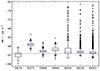 |
Fig. A.1. Boxplot of ionospheric corrected RM measurements of single pulses from PSR J0139+5814 taken on different days. The blue line in each box denotes the median. Each box spans for Inter-Quartile-Range. The horizontal dotted line is the literature RM value for the pulsar. The large number of outliers on MJDs 60303, 60336 and 60352 is due to the heightened ionospheric activity reported in the GMRT Cycle 45 observations. |
Appendix B: DPHASE variability
Rotational measurements are extremely sensitive to the cross-hand delay because the degeneracy described earlier. Therefore, we have to exercise extreme caution in measuring the delay and uncovering any systematics. GMRT being an interferometer where phasing operation is performed before every science scan, the DPHASE is susceptible to change on macroscopic variables (like ambient temperature and such). Investigating the underlying factors requires much more carefully planned study and is beyond the scope of this paper.
We plot the cross-hand delay we measure from scans of 3C138, noise diode and pulsar J0139+5814 against MJD, day-of-year and hour-of-day in Fig. B.1. The delay seems to vary from observation to observation. In almost all the cases, we only have a single measurement in an observation. However, observations of 12 Nov 2022 and 31 Dec 2022, we have noise diode scans and PSR J0139+5814 pulsar scans. The cross-hand delay measurement from all of them is consistent within an observation. The standard deviation of measurements of those observations is less than 0.1 ns. This can also be seen in the plot in the bottom panel where points follow a horizontal line.
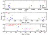 |
Fig. B.1. Cross-hand delay measurements from different scans: 3C138, noise diode, and PSR J0139+5814 plotted against MJD, day-of-year, and hour-of-day. The sign of the delay is purely a mathematical artifact. |
The fact that multiple delay measurements taken within an observation are consistent even with multiple phasings lends confidence to our RM measurements throughout the dataset. Alternatively, we investigate how much an error in cross-hand delay affects RM measurements. We take the B78 burst which was observed on MJD 59944. We construct multiple calibration solutions (PACV) files where GAIN and DGAIN are the same but only the cross-hand delay (Dns) is varied. We apply each calibration solution to the burst and perform RM measurement as mentioned in Sect. 3.3. We plot the cross-hand delay versus the measured RM in Fig. B.2. In the same figure, we plot the measured RM of B78 as red horizontal line and the black vertical line is the cross-hand delay used to calibrate this burst. We note that a 2 ns difference in the delay measurement causes 𝒪(10) difference in RM measurement. Nevertheless, as mentioned above, the variability we have seen in the delay measurement, which is less than 0.1 ns, does not affect our confidence in our measurements.
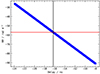 |
Fig. B.2. RM measurements when calibrating for different cross-hand delay. The black vertical line is the delay measurement from noise diode scan. The red horizontal line is the RM measurement. See text for details. |
All Tables
Band 4 Observations described in this paper (see the auxiliary material for a machine-readable csv file which include actual scan times).
All Figures
|
Fig. 1. Selection of polarization calibrated bursts. For each burst, we plot the de-dispersed dynamic spectra, frequency averaged total intensity (black) and RM corrected linear polarized (red) time series. The gray bands are RFI channels that have been zapped. The top left text in the time series panels is the burst ID. The rest of the plots can be found on zenodo. |
| In the text | |
|
Fig. 2. Rate over activity phase of FRB 20180916B. The horizontal dotted black line is the total average rate. The error bars and the shaded region around the horizontal dotted line correspond to 95% error. Top: Rate per phase for each observation color-coded by activity cycle of the source. Detections are marked by diamonds with 95% error bars. Nondetections are marked by triangles. Bottom: Rate over activity phase when all observations are considered (see text for more details). The down-pointing green triangles denote nondetection of bursts. The blue squares correspond to rates with 95% error, with y-axis toward the left. The red circles mark the total exposure at the corresponding phase with y-axis toward the right. |
| In the text | |
|
Fig. 3. Rate as a function of fluence for CHIME/FRB sample (Chime/Frb Collaboration 2020; Pleunis et al. 2021, in red) and our sample (in blue). Broken powerlaw are fitted to CHIME and our samples. The blue dotted lines are at 0.18 Jy ms and 1.10 Jy ms. The red dotted line is at 1.67 Jy ms. See text for the γ values. |
| In the text | |
|
Fig. 4. Time-aligned filterbank data of Band 4 (550–750 MHz) and Band 5 (1000–1200 MHz) showing simultaneous detections. The filterbank data has been de-dispersed to 1200 MHz (top of Band 5). The gray region is random data plotted to show continuity. The white strips are manually flagged RFI. The time-frequency resolution and color-scale have been suitable chosen to clearly display the bursts. |
| In the text | |
|
Fig. 5. Observed ionosphere corrected RM against MJD. CHIME/FRB RM23 are shown as red circles. LOFAR points are green diamonds AG23. This work’s points are plotted as blue squares. The dotted horizontal line is the reported RM before variability started (Nimmo et al. 2021). The dashed red line is the trend fitted by RM23. |
| In the text | |
|
Fig. A.1. Boxplot of ionospheric corrected RM measurements of single pulses from PSR J0139+5814 taken on different days. The blue line in each box denotes the median. Each box spans for Inter-Quartile-Range. The horizontal dotted line is the literature RM value for the pulsar. The large number of outliers on MJDs 60303, 60336 and 60352 is due to the heightened ionospheric activity reported in the GMRT Cycle 45 observations. |
| In the text | |
|
Fig. B.1. Cross-hand delay measurements from different scans: 3C138, noise diode, and PSR J0139+5814 plotted against MJD, day-of-year, and hour-of-day. The sign of the delay is purely a mathematical artifact. |
| In the text | |
|
Fig. B.2. RM measurements when calibrating for different cross-hand delay. The black vertical line is the delay measurement from noise diode scan. The red horizontal line is the RM measurement. See text for details. |
| In the text | |
Current usage metrics show cumulative count of Article Views (full-text article views including HTML views, PDF and ePub downloads, according to the available data) and Abstracts Views on Vision4Press platform.
Data correspond to usage on the plateform after 2015. The current usage metrics is available 48-96 hours after online publication and is updated daily on week days.
Initial download of the metrics may take a while.