| Issue |
A&A
Volume 694, February 2025
|
|
|---|---|---|
| Article Number | A91 | |
| Number of page(s) | 13 | |
| Section | Planets, planetary systems, and small bodies | |
| DOI | https://doi.org/10.1051/0004-6361/202452171 | |
| Published online | 05 February 2025 | |
Stellar obliquities of eight close-in gas giant exoplanets
1
Astronomical Institute of the Czech Academy of Sciences,
Fričova 298,
25165
Ondřejov,
Czech Republic
2
Faculty of Physics and Astronomy, Friedrich-Schiller-Universität,
Fürstengraben 1,
07743
Jena,
Germany
3
European Southern Observatory,
Karl-Schwarzschild-str. 2,
85748
Garching,
Germany
4
European Southern Observatory,
Casilla 13, Vitacura, Santiago,
Chile
5
Dipartimento di Fisica, La Sapienza Università di Roma,
Piazzale Aldo Moro 5,
Roma
00185,
Italy
6
Department of Theoretical Physics and Astrophysics, Masaryk Univesity,
Kotlářská 2,
60200
Brno,
Czech Republic
★ Corresponding author; This email address is being protected from spambots. You need JavaScript enabled to view it.
Received:
8
September
2024
Accepted:
9
January
2025
Abstract
The Rossiter–McLaughlin effect allows us to measure the projected stellar obliquity of exoplanets. From the spin-orbit alignment, planet formation and migration theories can be tested to improve our understanding of the currently observed exoplanetary population. Despite having the spin-orbit measurements for more than 200 planets, the stellar obliquity distribution is still not fully understood, warranting additional measurements to sample the full parameter space. We analyzed archival HARPS and HARPS-N spectroscopic transit time series of eight gas giant exoplanets on short orbits and derive their projected stellar obliquity λ. We report a prograde, but misaligned orbit for HAT-P-50b (λ = 41°−9+10), possibly hinting at previous high-eccentricity migration given the presence of a close stellar companion. We measure sky-projected obliquities that are consistent with aligned orbits for the rest of the planets: WASP- 48b (λ = −4° ± 4), WASP-59b (λ = 1°−21+20), WASP-140 Ab (λ = −1° ± 3), WASP-173 Ab (λ = 9° ± 5), TOI-2046b (λ = 1° ± 6), HAT-P-41 Ab (λ = − 4°−6+5), and Qatar-4b (λ = − 13°−19+15). We measure the true stellar obliquity ψ for four systems. We infer a prograde, but misaligned, orbit for TOI-2046b with ψ = 42−8+10 deg. Additionally, ψ = 30°−15+18 for WASP-140 Ab, ψ = 21°−10+9 for WASP-173 Ab, and ψ = 32°−13+14 for Qatar-4b. The aligned orbits are consistent with slow disk migration, ruling out violent events that would excite the orbits over the history of these systems. Finally, we provide a new age estimate for TOI-2046 of at least 700 Myr and for Qatar-4 of at least 350–500 Myr, contradicting previous results.
Key words: techniques: radial velocities / planets and satellites: atmospheres / planets and satellites: gaseous planets / planet–star interactions
© The Authors 2025
 Open Access article, published by EDP Sciences, under the terms of the Creative Commons Attribution License (https://creativecommons.org/licenses/by/4.0), which permits unrestricted use, distribution, and reproduction in any medium, provided the original work is properly cited.
This article is published in open access under the Subscribe to Open model. This email address is being protected from spambots. You need JavaScript enabled to view it. to support open access publication.
1 Introduction
Linking the observed exoplanetary population to the conditions in the protoplanetary disk is at the frontier of exoplanetary science. Exoplanetary atmospheres can provide a myriad of information on the system’s history (Madhusudhan 2019; Turrini et al. 2021). A complementary approach is to study the formation and evolution of exoplanetary systems through their dynamical parameters, that is the eccentricity, orbital period, and stellar obliquity1 (e.g., Turrini et al. 2020; Gajdoš & Vaňko 2023): we can indeed attempt to link the observed parameters of the planetary systems to the properties of their host stars and the environments in which they have formed (e.g., Öberg et al. 2011; Best & Petrovich 2022; Eistrup 2023; Gupta et al. 2024). In order to perform these studies with high significance, we need to measure these quantities over a wide range of parameter space.
The projected stellar obliquity (λ) is most commonly measured through the Rossiter–McLaughlin (R–M) effect – a spectroscopic anomaly that occurs when the disk of a companion passes in front of the spinning star. Currently, there are more than 215 measurements2 of the projected obliquity. Initially, the obliquity had been measured for hot Jupiters only, but advances in instrumentation (Mayor et al. 2003; Pepe et al. 2021; Seifahrt et al. 2022) have allowed the measurement of the spin-orbit alignment for Neptunian, sub-Neptunian, and even terrestrial planets. Such studies have revealed a complex architecture of exoplanetary systems with planetary orbits varying from well-aligned to slightly misaligned, and to planets on polar and even retrograde orbits. A more detailed description of the R–M effect is given in Triaud (2018) and Albrecht et al. (2022).
Misaligned and polar orbits are often thought of as indications of a violent history within the system as they contradict the standard formation processes where the planet and the star form from the same rotating disk. Hence, to explain these orbits, violent mechanisms, such as long-term interactions with a binary companion (Batygin 2012), close fly-bys of other stars (Bate et al. 2010), shifts of the stellar rotation axis relative to the disk due to the stellar magnetic field (Lai et al. 2011), gravitational scatterings among the planets (Chatterjee et al. 2008), or longterm perturbations due to a companion caused by Kozai-Lidov mechanism (Fabrycky & Tremaine 2007), are required.
The majority of stars are formed in binary or higher-multiplicity systems (Raghavan et al. 2010; El-Badry 2024). In addition to the spin-orbit orientation (between a planet and its host star3), orbit–orbit orientation (between the two components in a binary system) allows for more in-depth investigation of how the binary system could have formed (e.g., Rice et al. 2023). Several trends were identified in the exoplanetary population around host stars in binary pairs. In particular, Su et al. (2021) identified a population of massive short-period planets in close binaries that are almost absent in wide binaries or single stars. Some of the proposed explanations of this trend include enhanced planetary migration, collisions, and/or ejections in close binaries. Those are the same mechanisms that are also suggested for exciting the stellar obliquities of planetary systems. However, the exact role of stellar companions and planetary disks is not fully understood and requires further investigation to apprehend their interplay and the observed population (Barber et al. 2024).
The unprecedented astrometric sensitivity of the Gaia mission (Gaia Collaboration 2023) has allowed for the systematic study of both spin-orbit and orbit–orbit study (Christian et al. 2024). Rice et al. (2024) have studied the obliquity of 48 systems hosting an exoplanet and being part of a binary or triple system. From the observed line-of-sight orbit–orbit alignment and under-abundance of face-on systems that correspond to near-polar binary configuration, they suggest this might be due to viscous dissipation induced by nodal recession during the protoplanetary disk phase. Furthermore, they report that there is no clear correlation between spin-orbit misalignment and orbit–orbit misalignment, as initially reported by Behmard et al. (2022). However, further measurements are needed, as the sample is still quite limited.
In this study, we present, based on unpublished HARPS and HARPS-N archival data, the projected obliquity measurements of eight gas giants on short orbits around FGK dwarfs. At least five of them are part of binary or triple systems and three are astrometrically resolved.
2 Data sets and their analyses
2.1 Datasets
Our datasets come from two sources: two datasets (WASP-140 A and WASP-173 A) come from the HARPS instrument (Mayor et al. 2003) mounted at the ESO 3.6-m telescope at La Silla, Chile. The rest of the targets come from the HARPS-N instrument (Cosentino et al. 2012), mounted at the 3.58-m TNG telescope at La Palma, Canary Islands. The HARPS data were obtained from the ESO science archive4: program IDs 0102.C-0618(A), PI: Esposito; 0102.C-0319(A), PI: Anderson; while the HARPS-N data were obtained from the TNG archive5: program IDs CAT16B-119, PI: González; CAT17B-155, PI: Murgas Alcaíno; CAT18A-S, PI: IAC Service; OPT16A-49, PI: Ehrenreich, and CAT22A-9, PI: Orell. Table E.1 in the Appendix shows the properties of the data sets that were used. The downloaded data are fully reduced products as processed with the HARPS Data Reduction Software (DRS version 3.8). Each spectrum is provided as a merged 1D spectrum resampled onto a 0.001 nm uniform wavelength grid. The wavelength coverage of the spectra spans from 380 to 690 nm, with a resolving power of R ≈ 115 000, corresponding to 2.7 km s−1 per resolution element. The spectra are already corrected to the Solar system barycentric frame of reference. We further summarize the properties of the studied systems in Table 1.
2.2 Rossiter-–McLaughlin effect
The R-M effect causes a spectral line asymmetry, or, equivalently, an asymmetry in the cross-correlation function (CCF) that manifests as anomalous radial velocities during the transit of the exoplanet. We obtained the radial velocity measurements acquired from the HARPS and HARPS-N DRS pipelines together with their uncertainties. We combined the results from two nights when available. To measure the projected stellar obliquity of the system (λ), we followed the methodology of Zak et al. (2024a): we fitted the RVs with a composite model, which includes a Keplerian orbital component as well as the R-M anomaly. This model is implemented in the AROMEPY6 (Sedaghati et al. 2023) package, which utilizes the RADVEL python module (Fulton et al. 2018) for the formulation of the Keplerian orbit. AROMEPY is a Python implementation of the R–M anomaly described in the AROME code (Boué et al. 2013). We used the R–M effect function defined for RVs determined through the cross-correlation technique in our code. We set Gaussian priors for the RV semi-amplitude (K) and the systemic velocity (Γ). In the R–M effect model, we fixed the following parameters to values reported in the literature: the orbital period (P), the planet-to-star radius ratio (Rp /Rs), and the eccentricity (e). The parameter σ, which is the width of the CCF and represents the effects of the instrumental and turbulent broadening, was measured on the data and fixed. Furthermore, we used the ExoCTK7 tool to compute the quadratic limb-darkening coefficients with ATLAS9 model atmospheres (Castelli & Kurucz 2003) in the wavelength range of the HARPS and HARPS-N instruments (380–690 nm). We set Gaussian priors using the literature value and uncertainty derived from transit modeling (Table 1) on the following parameters during the fitting procedure8: the central transit time (TC), the orbital inclination (i), and the scaled semi-major axis (a/Rs). Uniform priors were set on the projected stellar rotational velocity (ν sin i*) and the sky-projected angle between the stellar rotation axis and the normal of the orbital plane (λ). To obtain the best fitting values of the parameters, we employed three independent Markov chain Monte Carlo (MCMC) ensemble simulations using the INFER9 implementation using the Affine-Invariant Ensemble Sampler. We initialized the MCMC at parameter values found by the Nelder-Mead method perturbed by a small value. We used 20 walkers each with 12 500 steps, burning the first 2 500. As a convergence check, we ensured that the Gelman-Rubin statistic (Gelman & Rubin 1992) is less than 1.001 for each parameter. Using this setup we obtain our results and present them in Sect. 3 and in Figs. 1 to E7 in the Appendix.
3 Projected stellar obliquities of eight gas giants
We measured the projected stellar obliquity (λ) of seven targets for the first time: WASP-48b, WASP-59b, WASP-140 Ab, WASP-173 Ab, TOI-2046b, HAT-P-50b, and Qatar-4b. HAT-P41 Ab has been previously studied by Johnson et al. (2017).
WASP-48b is an inflated hot Jupiter orbiting a G0V host star on a short 2.1-day orbit. The system potentially includes a wide stellar companion with ΔKs = 7.3 ± 0.1 (Ngo et al. 2016). The planet’s atmosphere has been studied by Murgas et al. (2017), who derived a flat transmission spectrum using the OSIRIS instrument mounted at the GTC. Recently, Bennett et al. (2023) used the HPF spectrograph at the Hobby–Eberly Telescope to report a non-detection of the helium feature that hints at a low planetary mass-loss rate. In our analysis, we infer an aligned orbit of WASP-48b with λ = −4 ± 4 deg.
WASP-59b is a warm Jupiter orbiting a K5 host star on a 7.95-day orbit. Fontanive & Bardalez Gagliuffi (2021) identified, using Gaia data, a wide (>9000 au) co-moving companion. We infer a prograde orbit with a broad but symmetric posterior in λ around alignment, with  deg.
deg.
WASP-140 Ab is a hot Jupiter orbiting a K0 host star on a 2.2-day orbit. The host star has a two magnitudes fainter companion, WASP-140 B, with a separation of 7″.24 ± 0″.01 and a position angle of 77.4 ± 0.1°, corresponding to a projected separation of 850 au. We infer an aligned orbit of WASP-140 Ab with λ = −1 ± 3 deg.
WASP-173 Ab is a massive hot Jupiter orbiting a G3 host star on a 1.4-day orbit (Hellier et al. 2019; Labadie-Bartz et al. 2019). The host star has a slightly less massive companion, WASP-173 B, with a separation of 6″.1 ± 0″.01 and a position angle of 110.1 ± 0.5°, corresponding to a projected separation of 1440 au. We infer an aligned orbit of WASP-173 Ab with λ = 9 ± 5 deg.
TOI-2046b is a hot Jupiter orbiting an F8 host star on a 1.5-day orbit. The reported age of the system between 100 and 400 Myr as determined from gyrochronology and the lithium method (Kabáth et al. 2022) would make it an amenable target for atmospheric escape study. Recently, Orell-Miquel et al. (2024) reported upper limits for Hα and He I excess absorption. We infer an aligned orbit of TOI-2046b with λ = 1 ± 6 deg., and show below that the star is likely much older.
HAT-P-41 Ab is an inflated hot Jupiter. It orbits its F6 host star on a 2.7-day orbit. Bohn et al. (2020) confirmed the binary companion HAT-P-41 B with a separation of 3″.621 ± 0″.004 and a position angle of 183.9 ± 0.1°, corresponding to a projected separation of 1240 au. Sheppard et al. (2021) reported high metal enrichment in the planetary atmosphere from Hubble Space Telescope’s (HST) transit spectroscopy; a result later confirmed by Jiang et al. (2024) with GTC/OSIRIS. In our analysis, we infer an aligned orbit with  deg. The stellar obliquity of HAT-P-41 Ab has been previously studied with the Doppler tomography method by Johnson et al. (2017) using the High-Resolution Spectrograph mounted at the Hobby-Eberly Telescope. They reported a prograde but slightly misaligned orbit with
  deg. Our result points at a more aligned orbit, but both results are consistent within 3 sigmas. Furthermore, as noted in Johnson et al. (2017), after the subtraction of their best fit model significant residuals remain and the authors have inflated their uncertainties by a factor of 2.5 to better account for possible systematics. We applied the Doppler shadow method on HARPS-N data in Appendix B deriving
  deg consistent with our classical R-M effect analysis.
HAT-P-50b is a hot Jupiter orbiting its F7 host star on a 3.1-day orbit (Hartman et al. 2015). Lester et al. (2021) reported the presence of a close binary companion with a separation of 0″.67 and a position angle of 321.1°, corresponding to a projected separation of 327 au. Due to the proximity the binary system is not astrometrically resolved in the Gaia DR3 data. We derive a prograde, yet misaligned, orbit with  deg.
deg.
Qatar-4b is a massive hot Jupiter. It orbits a supposedly moderately young (170 ± 10 Myr; but see below) K1 host star on a 1.8-day, possibly slightly eccentric (e = 0.06), orbit. We find that the orbit of Qatar-4b is well aligned, with  deg.
deg.
For all the stars considered, the obtained v sin i* values in our R-M effect analysis are in 3-σ agreement with the ones reported in the literature from the spectral synthesis. The largest discrepancy is observed for WASP-48. Hence, we measured the v sin i* from our HARPS-N stacked spectra, using iSpec (Blanco-Cuaresma et al. 2014). We obtain a value of v sin i* = 11.0 ± 0.6 km/s, in a better agreement with the value obtained from our R–M effect analysis in Table E.2.
The results of our fits are shown in Figs. 1 and E1–E7, while the MCMC results are shown in Appendix that is available on Zenodo (see Data availability). The derived values from the MCMC analysis are displayed in Table E.2 in the Appendix.
Properties of the targets (star and planet).
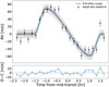 |
Fig. 1 Rossiter–McLaughlin effect of WASP-48b observed with HARPS-N. The observed data points (black) are shown with their error bars. The systemic and Keplerian orbit velocities were removed. The blue line shows the best fitting model to the data, together with 1-σ (dark grey) and 3-σ (light grey) confidence intervals. |
4 Discussion
4.1 Stellar rotation and true obliquity ψ
By detecting variations in the light curve, we can determine the stellar rotation periods (e.g., Skarka et al. 2022). This is crucial for estimating the stellar inclination i*, which in turn helps to determine the true obliquity. We attempted to derive the stellar rotation periods by analyzing ASAS-SN g-band light curves (Kochanek et al. 2017) using a Lomb-Scargle periodogram (Lomb 1976; Scargle 1982). We were able to detect a periodic modulation of WASP-140 A with a period of 10.44 ± 0.05 days (with False Alarm Probability (FAP)=1.6 × 10⁻¹¹), in agreement with the rotational period of 10.4 ± 0.1 days reported by Hellier et al. (2017) using Wide Angle Search for Planets (WASP) survey data. For Qatar-4, we detect a period of 7.07 ± 0.08 days (FAP=1.6 × 10⁻⁹). For WASP-173 A, we detect a period of 7.97 ± 0.05 days (FAP=1.6 × 10⁻¹²), also in agreement with the rotational period of 7.9 ± 0.1 days reported by Hellier et al. (2019) from WASP data. Furthermore, we have explored TESS data (Ricker et al. 2015) in search of rotational modulation. TOI-2046 was observed in 7 sectors. We detect a periodic modulation of TOI-2046 with a period of 4.05 ± 0.05 days (FAP=10 × 10−9 ) from the long cadence data in 3 sectors and a period of 4.29 ± 0.05 days (FAP=10 × 10−4) using the short cadence data in four different sectors. Such variability is present in many F-type stars showing rotational variability (e.g., Henriksen et al. 2023). Due to the higher signal-to-noise ratio detection, we adopt the former period. This periodicity, that we assume to be due to differential rotation, was not detected in the ASAS-SN data due to the small amplitude. For the other targets, we were not able to detect any signal with high significance. The phase curves figures of the four stars with detected rotational variability are available on Zenodo (see Data availability).
From the derived rotational periods we derived the equatorial velocity veq of 4.2 ± 0.2 km/s for WASP-140 A, 7.0 ± 0.4 km/s for WASP-173 A, 15.1 ± 1.1 km/s for TOI-2046, and 6.1 ± 0.5 km/s for Qatar-4. These values are in good agreement with the v sin i* values reported in Tables 1 and E.2. The different methods of deriving the rotational velocities might produce slight variations as, for example, the spectral synthesis method might not be able to distinguish various broadening mechanisms as opposed to the values derived from the R-M effect analysis that should provide only the rotational velocity. Another origin of the small variations can be a differential rotation of the star. Reinhold et al. (2013) found that the differential rotation increases with effective temperature and above 6000 K can be quite scattered. For example, if a planet is transiting over high stellar latitudes, the derived v sin i* may be lower compared to the rotational velocity originating from stellar spots in lower latitudes where the rotation is faster. Finally, as thoroughly discussed in Brown et al. (2017), the Boué model (Boué et al. 2013) for the Rossiter–McLaughlin effect, which we employed and that was developed to be used with instruments like HARPS, is known to provide a lower value of v sin i* compared to other models such as the Hirano model (Hirano et al. 2011) developed for the iodine cell or the Doppler shadow method (Collier Cameron et al. 2010), yet they agree on the derived projected obliquity value.
For these four planets, we are thus able to infer the true stellar obliquity ψ (i.e., the angle between the stellar spin-axis and the normal to the orbital plane) using the spherical law of cosines, cos ψ = sin i* sin i cos |λ| + cos i* cos i with the approach suggested by Masuda & Winn (2020) accounting for the dependency between v and v sin i*. We obtain  deg for WASP-140 Ab,
  deg for WASP-173 Ab,
  deg for TOI-2046b, and
  deg for Qatar-4b. From the true obliquity measurements, TOI-2046b shows a rather misaligned orbit. For the rest of the targets we can conclude that the orbits are clearly prograde, yet not exactly aligned with their host stars, although the misalignment that we measure is not statistically significant. In the following sections, we discuss the tidal alignment timescale and how the R–M effect and atmospheric characterization are in high synergy to unravel the history of the system.
4.2 Obliquity of young systems
The stellar obliquities of young systems are still not well characterized. There are only a handful of obliquity measurements for systems with ages below 200 Myr. These young systems offer a unique opportunity to study the primordial misalignment as, generally, the tidal forces have not had enough time to alter the architecture of the system. Currently, all the planets younger than 200 Myr seem to be well aligned with their host stars (Albrecht et al. 2022). Qatar-4 with a reported age of 170 ± 10 Myr (Alsubai et al. 2017) and TOI-2046 with its reported age between 100–400 Myr (Kabáth et al. 2022) would have been valuable additions to the few known systems. In Appendix C, we determined the age of Qatar-4 and TOI-2046 with several methods (lithium depletion, gyrochronology and R′HK index) and we provide evidence for Qatar-4 to be at least 350–500 Myr old and TOI-2046 being at least 700 Myr old. Hence, they do not belong to the moderately young population of exoplanets below 200 Myr.
4.3 Dynamical timescale
To better understand the evolution of the studied systems and their relevance, here we compare the age of the system and the tidal alignment timescale that can be used to study whether the spin-orbit angle has changed since the formation of the system. It provides only a limit on the possible realignment as the spin-orbit misalignment does not have to happen at the same time as the system’s formation. For cool stars below the Kraft break (Kraft 1967, that is, with convective envelopes), the tidal alignment timescale can be approximated (Albrecht et al. 2012) as
 (1)
(1)
This allows us to compute the tidal alignment timescale for all the studied planets but HAT-P-41 Ab, and derive the following timescales: τCe = 4 · 1010 yr for WASP-48b, 4 · 1014 yr for WASP- 59b, 1 · 1011 yr for WASP-140 Ab, 3 · 109 yr for WASP-173 Ab, 5 · 1010 yr for TOI-2046b, 8 · 1010 yr for HAT-P-50b, and 1 · 1010 yr for Qatar-4b.
HAT-P-41 A, with its spectral type F6, is classified as a hot star and thus lies above the Kraft break, having a radiative envelope – this structural difference has implications on the tidal forces and a different formula of the tidal alignment timescale (Albrecht et al. 2012) should be used:
 (2)
(2)
leading to τRA = 2 · 1015 yr for HAT-P-41 Ab.
Due to its short orbital period and large mass, WASP-173 Ab is likely older than its tidal alignment timescale and, hence, the high-eccentricity migration scenario cannot be ruled out from the stellar obliquity measurements alone. From the derived tidal alignment timescales of the rest of the planets, we can conclude that the current spin-orbit angles were likely not significantly changed from their initial values through tidal forces.
The only misaligned planet in our sample is HAT-P-50b. Given the reported presence of a close companion, this would be consistent with high-eccentricity migration via the Kozai-Lidov mechanism (Fabrycky & Tremaine 2007). We have therefore estimated the Kozai-Lidov timescale τKL to check whether such a scenario is viable, using the following formula (Naoz 2016):
 (3)
(3)
where MA and MB are the masses of the primary and secondary components of the binary system, PB is the orbital period of the binary system, Pb the orbital period of the exoplanet and eB the eccentricity of the binary pair. We have used values of MB=0.62 M⊙ and PB =4 440 yr (Lester et al. 2021). As the eccentricity of the binary system remains unconstrained, we calculate the τKL for values of eB between 0 to 0.9, leading to τKL ∼ 1 Gyr for eB=0 and τKL ∼ 0.1 Gyr for eB=0.9. From the derived values and their comparison to the age of the system of  Gyr (Hartman et al. 2015), we find that the Kozai-Lidov mechanism has possibly had enough time to change the orbital configuration of the system. Additionally, this timescale would be even shorter in the likely scenario that the planet has formed on a wider than currently observed orbit. To further confirm this orbital evolution hypothesis, measurements of the planetary atmospheres are warranted (Penzlin et al. 2024), but as shown in Table D.1 in the Appendix, HAT-P-50b is rather not an amenable target for atmospheric studies.
The low values of the spin-orbit angle of the remaining planets are consistent with slow disk migration (Baruteau et al. 2014). Planets undergoing disc migration are expected to have a distinct composition to those arriving via high-eccentricity migration (Kirk et al. 2024) and we comment on the future atmospheric prospects of HAT-P-41 Ab in the section D of the Appendix.
We show the comparison with the rest of the population in Fig. 2. HAT-P-50b lies in the less populated region of Hot Jupiters with misaligned orbits. These planets are important pieces in unraveling whether misaligned planets are distributed isotropically as suggested by Dong & Foreman-Mackey (2023) and Siegel et al. (2023) or whether the misaligned population shows a preference for polar and retrograde orbits as suggested by Albrecht et al. (2021) and Attia et al. (2023). Furthermore, HAT-P-50 lies on the position of the metallicity-dependent Kraft break as derived by Spalding & Winn (2022) where convective envelopes persist in a lower metallicity environment for slightly higher temperatures. The rest of our targets join the large population of Hot Jupiters on prograde and aligned orbits around their host stars.
As discussed in Hellier et al. (2017), WASP-140 Ab has a very short circularisation timescale, τcir, estimated to be between ~1 and 100 Myr (for a quality factor Qp = 105 and 106, respectively), hence a circular orbit is expected. However, the system retains a small but non-zero eccentricity. A recent migration event could explain the non-circular orbit, together with  derived above. Another plausible explanation is that an outer planetary companion in the WASP-140 A system is dynamically maintaining the non-zero eccentricity. This hypothesis makes the WASP-140 A system an excellent target for further investigation to resolve this ambiguity.
4.4 Obliquity in multi-star systems
The spin-orbit alignment is being investigated in multi-star systems to understand how planets form and evolve in binary systems and how the presence of the binary companion affects the proto-planetary disk environment (Christian et al. 2024). This can be done by investigating the orbital orientation between exoplanets and wide-orbiting binary companions. Christian et al. (2024) reported the existence of an alignment between the orbits of small planets and binary systems with semimajor axes below 700 au. Rice et al. (2024) have studied the obliquity distribution of multi-star systems. They reported no clear correlation between spin-orbit misalignment and orbit– orbit misalignment. Furthermore, they reported the discovery of an overabundance of systems that are consistent with joint orbit–orbit and spin–orbit alignment.
In the sample presented here, three planets are in astro- metrically resolved binary systems: WASP-140, WASP-173 and HAT-P-41. This allows us to compute the orbit–orbit angle γ using Gaia DR3 data:
 (4)
(4)
where r ≡ [Δα, Δδ] and ![Mathematical equation: ${\bf{\v }} \equiv \left[ {\Delta \mu _\alpha ^*,\Delta {\mu _\delta }} \right]$](/articles/aa/full_html/2025/02/aa52171-24/aa52171-24-eq30.png) . Here, Δα and Δδ denote the positional differences between the primary and secondary in the right ascension (RA) and declination (Dec) directions, while
. Here, Δα and Δδ denote the positional differences between the primary and secondary in the right ascension (RA) and declination (Dec) directions, while  and Δμδ are the proper motion differences in the RA and Dec directions. Gaia DR3 reports a
  value that has already the cos δ corrective factor in the RA direction incorporated10 (Rice et al. 2024).
The angle γ quantifies the alignment between a binary system’s relative position vector, r, and relative velocity vector, v. Values of γ near 0° or 180° suggest that the binary’s motion is predominantly along our line of sight, characteristic of an edge-on orientation (orbit–orbit alignment). Conversely, γ values near 90° indicate motion primarily perpendicular to our line of sight, aligning with a face-on orientation (orbit–orbit misalignment). However, interpreting γ for individual systems involves complexities: orbital eccentricity can cause variations in r and v that affect γ. Furthermore, the planet-hosting star can be oriented in within the sky-plane hence accurately determining the alignment between the planetary orbit and the binary orbit is difficult. Therefore, while γ offers insights into the system’s geometry, caution is necessary when interpreting its value due to these potential degeneracies. Significant improvements will be brought by the next Gaia data releases as the current astrometry data are based solely on 34 months of observations (Gaia Collaboration 2023).
For WASP-140 Ab, we infer a well-aligned spin-orbit angle of λ = −1 ± 3 deg. Furthermore, we derive an almost face-on orbit-orbit orientation with γ = 80.3 ± 6.3 deg and a binary inclination of 78.8 ± 5.9 deg. For WASP-173 Ab we derive a well-aligned orbit with λ = 9 ± 5 deg; additionally, we derive the orbit-orbit orientation of γ = 136.8 ± 4.2 deg and a binary inclination of 65.1 ± 7.0 deg. Finally, our R-M effect result  puts HAT-P-41 into the group of systems with spin-orbit alignment and orbit-orbit misalignment (γ = 72.7 ± 2.9 deg).
Since the study by Rice et al. (2024), two more systems in multi-star systems had their obliquity measured (WASP-77 and HD 110067). WASP-77 is a binary system with 1.00 ± 0.07 M⊙ and 0.71 ± 0.06 M⊙ components. The primary star hosts a hot Jupiter on a 1.4-day orbit (Maxted et al. 2013). Zak et al. (2024a) reported  deg for WASP-77 Ab. Using Gaia DR3 astrometry (Gaia Collaboration 2023), we can now also compute the orbit-orbit alignment, γ = 14.4 ± 12.1 deg, together with the binary inclination of 86.5 ± 15.1 deg. Hence, the WASP-77 system joins 8 other systems identified by Rice et al. (2024) that also show such a high degree of alignment. HD 110067 hosts six transiting sub-Neptunes in resonant chain orbits. The primary has an equal mass binary companion at separation of 13 400 au making this a triple system with the highest number of known exoplanets (Luque et al. 2023; Apps & Luque 2023). Zak et al. (2024b) inferred an aligned orbit for HD 110067c with
  deg. We now report also the orbit-orbit alignment of γ = 156.5 ± 23.2 deg, hinting at a possible slight deviation from a fully edge-on orbit.
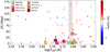 |
Fig. 2 Projected obliquity versus stellar effective temperature. Our targets are plotted with squares. The gray area shows the position of the Kraft break as derived in Spalding & Winn (2022). The literature values were retrieved from the TEPCat catalogue (Southworth 2011). |
5 Summary
Understanding the spin-orbit orientation in compact systems and how planetary orbits align or misalign with the orbits of multi-star systems and what pathways these planets might follow to achieve their observed configuration (e.g., the reported preference for line-of-sight orbit–orbit alignment) still remains unanswered. To improve our understanding of these pathways we studied the projected stellar obliquity of eight gas giants on short orbits around FGK stars with five systems being part of multi-star systems. From the archival HARPS and HARPS-N data, we measured the Rossiter–McLaughlin effect and infer the projected spin-orbit alignment of WASP-40b, WASP-59b, WASP-140 Ab, WASP-173 Ab, TOI-2046b, HAT-P-50b, and Qatar-4b for the first time and we update the value for HAT-P41 Ab using a new dataset. We report a prograde but misaligned orbit for HAT-P-50b  consistent with a Kozai-Lidov mechanism triggered by the close stellar companion. We derive potentially aligned orbits for the rest of the studied systems ruling out highly excited orbits due to the presence of stellar companions. For four systems, we also derive their true (3-D) obliquity with TOI-2046b having a misaligned orbit with
  deg. Additionally, we derive
  deg for WASP-140 Ab,
  deg for WASP-173 Ab, and
  deg for Qatar-4b. We provide a refined age estimate for the previously reported moderately young (100–400 Myr) system TOI-2046 and (~170 Myr) system Qatar-4; we rather conclude that the systems are at least 700 Myr and 350–500 Myr old, respectively. Finally, we report the orbit–orbit angle for five multi-star systems hosting exoplanets for the first time identifying two systems with line-of-sight orbit–orbit misalignment. Further studies of the spin-orbit orientation in multi-star systems are highly encouraged especially with the upcoming Gaia DR4 release coming in 2026 providing astrometry data based on 66 months of observations to enhance the orbit–orbit constraints.
Data availability
Phase curves of WASP-140, Qatar-4, WASP-173, and TOI-2046 showing rotational variability and corner plots of the MCMC analysis of the R-M effect of all systems are in Appendix that is available on Zenodo (https://zenodo.org/records/14633245).
Acknowledgements
The authors would like to thank the anonymous referee for their insightful report. JZ and PK acknowledge support from GACR:22-30516K. AB is supported by the Italian Space Agency (ASI) with Ariel grant no. 2021.5.HH.0. MS acknowledges the financial support of the Inter-transfer grant no. LTT-20015.
Appendix A TESS photometry of WASP-59
We analyzed photometric data of WASP-59 (TIC 91051152) using observations from TESS (Ricker et al. 2015). The target was observed in a single Sector 56, during September 2022 at a 120-second cadence. A total of three transits of WASP-59b were captured, which were used to improve the planetary transit parameters. We utilized the Pre-search Data Conditioning SAP (PDCSAP) flux, which provides light curves corrected for instrumental systematics and stellar variability. To model the observed transits, we employed the exoplanet package (Foreman-Mackey et al. 2021), a Bayesian framework for transit modeling.
The transit model assumed a Keplerian orbit and included a Gaussian Process (GP) to account for residual stellar variability. The stellar radius (R⋆) was constrained with a Gaussian prior centered on the value reported by Hébrard et al. (2013). Similarly, the orbital period (P) was modeled using a Gaussian prior based on previously determined ephemeris values. The transit depth (δ) was also constrained with a Gaussian prior informed by earlier observations. A uniform prior between 0 and 1 was applied to the impact parameter (b). We adopted a quadratic limb-darkening law following Kipping (2013). The limb-darkening coefficients (u1 , u2) were sampled with uniform priors constrained to the range between 0 and 1. The eccentricity e and argument of periastron ω were fixed to values from Hébrard et al. (2013). To model residual stellar variability in the PDCSAP flux, we used a Matern-3/2 Gaussian Process kernel (Foreman-Mackey et al. 2017; Foreman-Mackey 2018). We initialized the model using estimates for the orbital period, planetary radius, and reference transit time obtained from a Box Least Squares (BLS) periodogram analysis. The model parameters were first optimized using the maximum a posteriori (MAP) estimate. This was followed by Markov Chain Monte Carlo (MCMC) sampling using the No-U-Turn Sampler (NUTS). We performed 2000 tuning steps and sampled the posterior distributions with 7000 draws using three independent ensembles ensuring R-hat  value below 1.001 for all parameters. The obtained results are in good agreement with the literature values and are shown in Table A.1 and the phase curve shown in Fig. A.1.
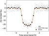 |
Fig. A.1 Phase curve of WASP-59b using TESS data centered around the primary transit. Observed data are shown in gray, binned data in black and the obtained transit model in orange color. |
Obtained parameters of WASP-59b from fitting TESS data.
Appendix B Doppler Shadow of HAT-P-41 Ab
Doppler tomography, a technique (Collier Cameron et al. 2010) used to measure the stellar obliquity independently on the classical method provides a high-fidelity representation of the integrated stellar line profile, which is essential for detecting distortions induced during a planetary transit. By subtracting individual in-transit CCFs from a master out-of-transit CCF, which represents the underlying Gaussian-approximated line shape, one can isolate the characteristic time-varying distortion, known as the “Doppler shadow.” This shadow encodes valuable information about the projected rotational velocity of the stellar surface (v sin i∗) and the sky-projected obliquity (λ). We analyzed HARPS-N data of HAT-P-41. Using the Doppler tomography method, we successfully detected the Doppler shadow, as shown in Figure B.1. To fit the shadow of HAT-P-41 Ab, we employed TRACIT, a Python module11 developed and described in Knud- strup & Albrecht (2022) that implements MCMC method.
Setting a uniform uninformative prior on λ did not allow us to meaningfully distinguish between the results from Johnson et al. (2017) and the results we previously derived. Hence, we set a Gaussian prior on λ to -13.1 deg as the mean value between the λ from Johnson et al. (2017), and the one that we previously derived using the classical RM effect. The same approach was applied for v sin i∗, where we set the central value 17.7 km/s (the mean of 19.6 and 15.8 km/s), coming from mentioned sources, respectively. We ran three independent MCMC realizations using 100 walkers with 12000 draws, burning 6000 with the corner plot shown in Fig. B.2. The priors we used are listed in Table B.1, together with the obtained results. The used values for microturbulence ζ, and macroturbulence ξ velocities utilized were taken from Bruntt et al. (2010) and Doyle et al. (2014), respectively. The limb darkening values q1 and q2 were obtained from the ExoCTK tool. The Gelman-Rubin statistic for each parameter was below 1.004. The obtained result of  deg favors an aligned orbit of the planet in agreement with our classical R-M effect analysis.
Priors and results of the HAT-P-41 Ab Doppler shadow analysis.
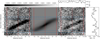 |
Fig. B.1 Doppler shadow analysis. Left: Doppler shadow of HAT-P-41 Ab as it appears in the observed data (depth is indicated by the upper, horizontal colorbar); middle: a best-fitting model of the Doppler shadow, right: residuals of the best-fitting model after subtraction from the actual data. The blue solid and dashed lines mark the boundaries for the full and total transit times, respectively. |
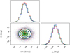 |
Fig. B.2 Corner plot representing the posterior distributions of the projected rotational velocity (v sin i∗) and projected obliquity (λ) of our Doppler Shadow analysis of HAT-P-41 Ab. Shown are three MCMC initializations. The result |

Appendix C Stellar ages
We tried to improve the age determination of the supposedly young stars TOI-2046 and Qatar-4 using the lithium method. Despite increasing the signal by stacking all the HARPS-N spectra, we report a non-detection of lithium in the stellar spectrum of both TOI-2046 and Qatar-4 (Fig. C.1). Hence, we can only derive lower age limits: using lithium models from Jeffries et al. (2023) for the given effective temperature of TOI-2046 and Qatar-4, we infer that TOI-2046 is at least 700 Myr old and Qatar-4 is at least 500 Myr old.
Additionally, we applied the R′HK index method. We measured the median value of log R′HK = −4.66 ± 0.01 for TOI-2046 and log R′HK = -4.53 ± 0.02 for Qatar-4. Using the calibrations from Mamajek & Hillenbrand (2008) we infer activity age of 1.6 ±0.1 Gyr for TOI-2046 and 0.75 ± 0.10 Gyr for Qatar-4.
Subsequently, we tried to infer the age of the Qatar-4 using isochrones. From the stacked spectra we determined the stellar parameters of Qatar-4. We have used the iSpec software (Blanco-Cuaresma et al. 2014; Blanco-Cuaresma 2019) together with MARCS atmosphere models (Gustafsson et al. 2008). We derive Teff =5220 ± 45 K, log 𝑔 = 4.49 ± 0.09, [Fe/H]= 0.09 ± 0.10 and v sini∗ = 5.7 ± 0.3 km/s. The derived parameters are in agreement with previous work using TRES spectra (Alsubai et al. 2017). Using the above-derived parameters as well as the Gaia magnitudes, we were not able to put any meaningful constraint on the age from only the isochrones fitting (Fig. C.2).
We have also determined the age of Qatar-4 using gyrochronology. The gyrochronology method employs the agerotation relation to infer the ages of stars. Such a method is based on the observations of stellar clusters that showed that stellar rotation slows down as the stars become older. First, we checked that the Renormalised Unit Weight Error (RUWE) value in the Gaia DR3 catalog is not above 1.25, which would imply a poor astrometric solution possibly hinting at an unresolved binary companion that could bias subsequent analysis. The retrieved RUWE value of 1.02 points towards a well-behaved astrometric solution. We have used the python package gyro-interp12 based on the work of Bouma et al. (2023). For the stellar rotational period and the effective temperature of Qatar-4, we derive an age of  Myr. As an independent check, we have also used the stardate13 python tool that combines isochrone fitting with gyrochronology (Angus et al. 2019). We derive an age of
  Myr. Hence, Qatar-4 does not appear to belong to the moderately young (< 200 Myr) population of stars hosting exoplanets. Following the same steps, we also derive an age of
  Gyr for TOI-2046, using the gyro-interp tool, and
  Gyr using stardate. Repeating -the steps we derive an age of 0.9 ± 0.1 Gyr for WASP-140, using the gyro-interp tool, and
  Gyr using stardate. Age determinations that rely on different methods (e.g., isochrone fitting, gyrochronology, lithium abundance, and chromospheric activity) can yield variations because each approach is sensitive to a distinct combination of stellar properties and evolutionary stages (e.g., Soderblom 2010). Isochrone fitting is often more robust for stars that have evolved off the Zero-Age Main Sequence. Gyrochronology, on the other hand, leverages the relationship between rotation period and age, which has been calibrated primarily for solar-like dwarfs in clusters of known ages (e.g., Bouma et al. 2024). As a consequence, this technique can suffer biases for stars that do not follow the standard spin-down tracks (e.g., due to tidal interactions, unusual magnetic activity, or past merging events) and is less reliable for F-type stars, which may spin down more slowly or exhibit weaker magnetic braking (van Saders et al. 2016). Similarly, lithium abundance can provide an age estimate by tracing depletion over time in G/K dwarfs, yet there is significant star-to-star scatter at a given age, and this method is more sensitive in younger populations when Li depletion is rapid (e.g., Jeffries et al. 2023). Chromospheric activity indices (e.g., R′HK) also correlate with stellar age, but the calibration has intrinsic scatter and may be affected by shortterm stellar variability and/or episodic activity cycles (Mamajek & Hillenbrand 2008). The differences found for TOI-2046 and Qatar-4 are therefore consistent with the typical systematic limitations of each technique. Nonetheless, the broad agreement among the various indicators is that these systems are older than previously reported.
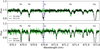 |
Fig. C.1 Spectral region around the lithium doublet (blue vertical lines) together with iron and calcium lines. The top panel shows stacked spectra of TOI-2046 (green) alongside with TOI-1135 (black) with similar spectral type and an age ~ 650 Myr (Mallorquín et al. 2024). The bottom panel shows stacked spectra of Qatar-4 (green) alongside with TOI-2048 (black) with similar spectral type and an age ~ 300 Myr (Newton et al. 2022). Both TOI-2046 and Qatar-4 show clear non-detection of the lithium hinting at an older age. |
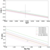 |
Fig. C.2 Isochrone fitting of Qatar-4. Top: H-R diagram, using effective temperature and luminosity of Qatar-4. Bottom: Gaia color-magnitude diagram. In both cases, the position of Qatar-4 is indicated, while the colored lines show distinct isochrones, as indicated in the legend. This clearly indicates that isochrones only cannot be used to derive a precise age. |
Appendix D Future atmospheric characterization
The composition of exoplanetary atmospheres can be used in a complementary way to study the formation and evolution of exoplanetary systems (Dawson & Johnson 2018). In particular, the elemental ratios (e.g., C/O, N/O, O/H, S/N) can be used to constrain the system’s history as well as to investigate the chemically diverse environment in protoplanetary disk (e.g., Turrini et al. 2021; Pacetti et al. 2022). Since the launch of the JWST, we have now more than a dozen systems with measured atmospheric composition with an unattainable precision a few years ago. This number will steadily grow in the future. These data will be complemented by the ESA Ariel mission (Tinetti et al. 2018) that will obtain homogeneous spectroscopic data for hundreds of atmospheres (Bocchieri et al. 2023). We computed the transmission and emission spectroscopy metric (Kempton et al. 2018) to assess which targets from our sample are the most amenable to future follow-up. As can be seen from Table D.1, the most amenable target for transmission spectroscopy is HAT-P-41 Ab.
Transmission (TSM) and emission (ESM) spectroscopy metrics for our sample.
The atmosphere of HAT-P-41 Ab has been studied by Sheppard et al. (2021) and Jiang et al. (2024), who reported one of the highest metallicities of the known hot Jupiters. Such a high metallicity (especially O/H) supports the migration of the planets through the disk via viscous torques over other mechanisms (disk-free migration or formation via pebble accretion whereby the oxygen-rich solids are locked in the core). As discussed in Sheppard et al. (2021), the previously reported moderately misaligned orbit of the HAT-P-41 Ab is in tension with the disk migration hypothesis. HAT-P-41 Ab was initially considered for detailed atmospheric study with JWST, however, due to the reported misalignment it has been withdrawn from the otherwise homogeneous sample (Kirk et al. 2024). Our value of  deg is in better agreement with the disk migration scenario where the planet has formed outside of the H2O snowline and migrated inward while accreting substantial mass in planetesimals.
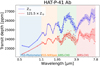 |
Fig. D.1 Simulated Ariel transmission spectrum of HAT-P-41 Ab’s atmosphere. The solid lines represent the unscattered spectra. The shaded colored areas correspond to the 1-σ confidence levels of the Ariel observations simulated in Tier 3 of the mission (Edwards et al. 2019). The dots are noisy data representing observed spectra. In red, we show a spectrum with enhanced metallicity, consistent with Sheppard et al. (2021). In blue, we show a spectrum with solar metallicity as derived by Changeat et al. (2022). Ariel will be able to distinguish between these two models with high confidence with three observed transits due to its broad wavelength coverage and high stability. |
However, the enhanced metallicity result was not confirmed by the independent analysis of the HST data by Changeat et al. (2022) who reported sub-solar to solar metallicity. The main limiting factor when deriving precise metallicity and the C/O ratio with the HST data is the narrow wavelength coverage of the HST and the presence of complex systematics (Gibson et al. 2011). Ariel will provide simultaneous coverage from 0.6 to 7.8 µm, allowing the determination of the chemical composition with high confidence. In Fig. D.1 we provide the Ariel simulated transmission spectrum of HAT-P-41 Ab obtained with three transits. We provide Ariel spectrum rather than one from JWST as a conservative estimate due to the smaller mirror diameter of Ariel. Ariel is set to perform a homogeneous study of hundreds of planetary atmospheres. We used the same setup (Mugnai et al. 2020; Mugnai et al. 2023) as in Zak et al. (2024a) to simulate the Ariel spectra. Ariel data will be able to unambiguously distinguish between solar-like and enhanced metallicity. The most prominent features for the metallicity determination are H2O and CO2. With a day-side temperature of ∼ 2300 K HAT-P-41 Ab lies in the transitional region between hot and ultra-hot Jupiters where physical processes such as molecular dissociation and H− opacity become important. By understanding the thermal structure of the atmosphere it will be possible to narrow down the onset conditions of these processes. The inferred well-aligned orbit of HAT-P-41 Ab would be consistent with the outcome of disk migration where the formation models expect an oxygen-rich atmosphere with high-atmospheric metallicity (Madhusudhan et al. 2014). High-confidence confirmation of the enhanced metallicity is hence important for testing our current planet formation models. If, on the other hand, sub-solar to solar metallicity is derived, consistently with the results by Changeat et al. (2022), this would hint at different processes at play.
Appendix E Additional tables and figures
Observing logs for all eight planets. The number in parenthesis represents the number of frames taken in-transit.
MCMC analysis results. 𝒩 denotes priors with a normal distribution and 𝒰 priors with a uniform distribution.
References
- Albrecht, S., Winn, J. N., Johnson, J. A., et al. 2012, ApJ, 757, 18 [NASA ADS] [CrossRef] [Google Scholar]
- Albrecht, S. H., Marcussen, M. L., Winn, J. N., et al. 2021, ApJ, 916, L1 [NASA ADS] [CrossRef] [Google Scholar]
- Albrecht, S. H., Dawson, R. I., & Winn, J. N. 2022, PASP, 134, 082001 [NASA ADS] [CrossRef] [Google Scholar]
- Alexoudi, X. 2022, Astron. Nachr., 343, e24012 [NASA ADS] [CrossRef] [Google Scholar]
- Alsubai, K., Mislis, D., Tsvetanov, Z. I., et al. 2017, AJ, 153, 200 [Google Scholar]
- Angus, R., Morton, T. D., Foreman-Mackey, D., et al. 2019, AJ, 158, 173 [Google Scholar]
- Apps, K., & Luque, R. 2023, RNAAS, 7, 264 [NASA ADS] [Google Scholar]
- Attia, O., Bourrier, V., Delisle, J. B., et al. 2023, A&A, 674, A120 [NASA ADS] [CrossRef] [EDP Sciences] [Google Scholar]
- Barber, M. G., Mann, A. W., Vanderburg, A., et al. 2024, Nature, 635, 574 [NASA ADS] [CrossRef] [Google Scholar]
- Baruteau, C., Crida, A., Paardekooper, S. J., et al. 2014, in Protostars and Planets VI, eds. H. Beuther, R. S. Klessen, C. P. Dullemond, et al., 667 [Google Scholar]
- Bate, M. R., Lodato, G., & Pringle, J. E. 2010, MNRAS, 401, 1505 [NASA ADS] [CrossRef] [Google Scholar]
- Batygin, K. 2012, Nature, 491, 418 [NASA ADS] [CrossRef] [Google Scholar]
- Behmard, A., Dai, F., & Howard, A. W. 2022, AJ, 163, 160 [NASA ADS] [CrossRef] [Google Scholar]
- Bennett, K. A., Redfield, S., Oklopcic, A., et al. 2023, AJ, 165, 264 [NASA ADS] [CrossRef] [Google Scholar]
- Best, S., & Petrovich, C. 2022, ApJ, 925, L5 [NASA ADS] [CrossRef] [Google Scholar]
- Blanco-Cuaresma, S. 2019, MNRAS, 486, 2075 [Google Scholar]
- Blanco-Cuaresma, S., Soubiran, C., Heiter, U., et al. 2014, A&A, 569, A111 [NASA ADS] [CrossRef] [EDP Sciences] [Google Scholar]
- Bocchieri, A., Mugnai, L. V., Pascale, E., et al. 2023, Exp. Astron., 56, 605 [NASA ADS] [CrossRef] [Google Scholar]
- Bohn, A. J., Southworth, J., Ginski, C., et al. 2020, A&A, 635, A73 [NASA ADS] [CrossRef] [EDP Sciences] [Google Scholar]
- Boué, G., Montalto, M., Boisse, I., et al. 2013, A&A, 550, A53 [NASA ADS] [CrossRef] [EDP Sciences] [Google Scholar]
- Bouma, L. G., Palumbo, E. K., & Hillenbrand, L. A. 2023, ApJ, 947, L3 [NASA ADS] [CrossRef] [Google Scholar]
- Bouma, L. G., Hillenbrand, L. A., Howard, A. W., et al. 2024, ApJ, 976, 234 [NASA ADS] [CrossRef] [Google Scholar]
- Brown, D. J. A., Triaud, A. H. M. J., Doyle, A. P., et al. 2017, MNRAS, 464, 810 [Google Scholar]
- Bruntt, H., Bedding, T. R., Quirion, P. O., et al. 2010, MNRAS, 405, 1907 [Google Scholar]
- Castelli, F., & Kurucz, R. L. 2003, in Modelling of Stellar Atmospheres, 210, eds. N. Piskunov, W. W. Weiss, & D. F. Gray, A20 [NASA ADS] [Google Scholar]
- Changeat, Q., Edwards, B., Al-Refaie, A. F., et al. 2022, ApJS, 260, 3 [NASA ADS] [CrossRef] [Google Scholar]
- Chatterjee, S., Ford, E. B., Matsumura, S., et al. 2008, ApJ, 686, 580 [Google Scholar]
- Christian, S., Vanderburg, A., Becker, J., et al. 2024, arXiv e-prints [arXiv:2405.10379] [Google Scholar]
- Collier Cameron, A., Guenther, E., Smalley, B., et al. 2010, MNRAS, 407, 507 [NASA ADS] [CrossRef] [Google Scholar]
- Cosentino, R., Lovis, C., Pepe, F., et al. 2012, SPIE Conf. Ser., 8446, 84461V [Google Scholar]
- Dawson, R. I., & Johnson, J. A. 2018, ARA&A, 56, 175 [Google Scholar]
- Dong, J., & Foreman-Mackey, D. 2023, AJ, 166, 112 [NASA ADS] [CrossRef] [Google Scholar]
- Doyle, A. P., Davies, G. R., Smalley, B., et al. 2014, MNRAS, 444, 3592 [NASA ADS] [CrossRef] [Google Scholar]
- Edwards, B., Mugnai, L., Tinetti, G., Pascale, E., & Sarkar, S. 2019, AJ, 157, 242 [NASA ADS] [CrossRef] [Google Scholar]
- Eistrup, C. 2023, ACS Earth Space Chem., 7, 260 [NASA ADS] [CrossRef] [Google Scholar]
- El-Badry, K. 2024, New A Rev., 98, 101694 [NASA ADS] [CrossRef] [Google Scholar]
- Enoch, B., Anderson, D. R., Barros, S. C. C., et al. 2011, AJ, 142, 86 [NASA ADS] [CrossRef] [Google Scholar]
- Fabrycky, D., & Tremaine, S. 2007, ApJ, 669, 1298 [NASA ADS] [CrossRef] [Google Scholar]
- Fontanive, C., & Bardalez Gagliuffi, D. 2021, Front. Astron. Space Sci., 8, 16 [NASA ADS] [CrossRef] [Google Scholar]
- Foreman-Mackey, D. 2018, RNAAS, 2, 31 [NASA ADS] [Google Scholar]
- Foreman-Mackey, D., Agol, E., Ambikasaran, S., et al. 2017, AJ, 154, 220 [NASA ADS] [CrossRef] [Google Scholar]
- Foreman-Mackey, D., Luger, R., Agol, E., et al. 2021, J. Open Source Softw., 6, 3285 [NASA ADS] [CrossRef] [Google Scholar]
- Fulton, B. J., Petigura, E. A., Blunt, S., et al. 2018, PASP, 130, 044504 [NASA ADS] [CrossRef] [Google Scholar]
- Gaia Collaboration (Vallenari, A., et al.) 2023, A&A, 674, A1 [NASA ADS] [CrossRef] [EDP Sciences] [Google Scholar]
- Gajdoš, P., & Vanko, M. 2023, MNRAS, 518, 2068 [Google Scholar]
- Gelman, A., & Rubin, D. B. 1992, Statist. Sci., 7, 457 [NASA ADS] [Google Scholar]
- Gibson, N. P., Pont, F., & Aigrain, S. 2011, MNRAS, 411, 2199 [Google Scholar]
- Gupta, A. F., Millholland, S. C., Im, H., et al. 2024, Nature, 632, 50 [NASA ADS] [CrossRef] [Google Scholar]
- Gustafsson, B., Edvardsson, B., Eriksson, K., et al. 2008, A&A, 486, 951 [NASA ADS] [CrossRef] [EDP Sciences] [Google Scholar]
- Hartman, J. D., Bakos, G. Á., Béky, B., et al. 2012, AJ, 144, 139 [NASA ADS] [CrossRef] [Google Scholar]
- Hartman, J. D., Bhatti, W., Bakos, G. Á., et al. 2015, AJ, 150, 168 [NASA ADS] [CrossRef] [Google Scholar]
- Hébrard, G., Collier Cameron, A., Brown, D. J. A., et al. 2013, A&A, 549, A134 [NASA ADS] [CrossRef] [EDP Sciences] [Google Scholar]
- Hellier, C., Anderson, D. R., Collier Cameron, A., et al. 2017, MNRAS, 465, 3693 [NASA ADS] [CrossRef] [Google Scholar]
- Hellier, C., Anderson, D. R., Bouchy, F., et al. 2019, MNRAS, 482, 1379 [CrossRef] [Google Scholar]
- Henriksen, A. I., Antoci, V., Saio, H., et al. 2023, MNRAS, 524, 4196 [NASA ADS] [CrossRef] [Google Scholar]
- Hirano, T., Suto, Y., Winn, J. N., et al. 2011, ApJ, 742, 69 [NASA ADS] [CrossRef] [Google Scholar]
- Jeffries, R. D., Jackson, R. J., Wright, N. J., et al. 2023, MNRAS, 523, 802 [NASA ADS] [CrossRef] [Google Scholar]
- Jiang, C., Chen, G., Murgas, F., et al. 2024, A&A, 682, A73 [NASA ADS] [CrossRef] [EDP Sciences] [Google Scholar]
- Johnson, M. C., Cochran, W. D., Addison, B. C., et al. 2017, AJ, 154, 137 [NASA ADS] [CrossRef] [Google Scholar]
- Kabáth, P., Chaturvedi, P., MacQueen, P. J., et al. 2022, MNRAS, 513, 5955 [CrossRef] [Google Scholar]
- Kempton, E. M. R., Bean, J. L., Louie, D. R., et al. 2018, PASP, 130, 114401 [Google Scholar]
- Kipping, D. M. 2013, MNRAS, 435, 2152 [Google Scholar]
- Kirk, J., Ahrer, E.-M., Penzlin, A. B. T., et al. 2024, RAS Tech. Instrum., 3, 691 [Google Scholar]
- Knudstrup, E., & Albrecht, S. H. 2022, A&A, 660, A99 [NASA ADS] [CrossRef] [EDP Sciences] [Google Scholar]
- Kochanek, C. S., Shappee, B. J., Stanek, K. Z., et al. 2017, PASP, 129, 104502 [Google Scholar]
- Kraft, R. P. 1967, ApJ, 150, 551 [Google Scholar]
- Labadie-Bartz, J., Rodriguez, J. E., Stassun, K. G., et al. 2019, ApJS, 240, 13 [NASA ADS] [CrossRef] [Google Scholar]
- Lai, D., Foucart, F., & Lin, D. N. C. 2011, MNRAS, 412, 2790 [NASA ADS] [CrossRef] [Google Scholar]
- Lester, K. V., Matson, R. A., Howell, S. B., et al. 2021, AJ, 162, 75 [NASA ADS] [CrossRef] [Google Scholar]
- Lomb, N. R. 1976, Ap&SS, 39, 447 [Google Scholar]
- Luque, R., Osborn, H. P., Leleu, A., et al. 2023, Nature, 623, 932 [NASA ADS] [CrossRef] [Google Scholar]
- Maciejewski, G. 2022, Acta Astron., 72, 1 [NASA ADS] [Google Scholar]
- Madhusudhan, N. 2019, ARA&A, 57, 617 [NASA ADS] [CrossRef] [Google Scholar]
- Madhusudhan, N., Amin, M. A., & Kennedy, G. M. 2014, ApJ, 794, L12 [Google Scholar]
- Mallorquín, M., Lodieu, N., Béjar, V. J. S., et al. 2024, A&A, 685, A90 [NASA ADS] [CrossRef] [EDP Sciences] [Google Scholar]
- Mamajek, E. E., & Hillenbrand, L. A. 2008, ApJ, 687, 1264 [Google Scholar]
- Masuda, K., & Winn, J. N. 2020, AJ, 159, 81 [NASA ADS] [CrossRef] [Google Scholar]
- Maxted, P. F. L., Anderson, D. R., Collier Cameron, A., et al. 2013, PASP, 125, 48 [NASA ADS] [CrossRef] [Google Scholar]
- Mayor, M., Pepe, F., Queloz, D., et al. 2003, The Messenger, 114, 20 [NASA ADS] [Google Scholar]
- Mugnai, L. V., Bocchieri, A., & Pascale, E. 2023, J. Open Source Softw., 8, 5348 [NASA ADS] [CrossRef] [Google Scholar]
- Mugnai, L. V., Pascale, E., Edwards, B., et al. 2020, Exp. Astron., 50, 303 [NASA ADS] [CrossRef] [Google Scholar]
- Murgas, F., Pallé, E., Parviainen, H., et al. 2017, A&A, 605, A114 [NASA ADS] [CrossRef] [EDP Sciences] [Google Scholar]
- Naoz, S. 2016, ARA&A, 54, 441 [Google Scholar]
- Newton, E. R., Rampalli, R., Kraus, A. L., et al. 2022, AJ, 164, 115 [Google Scholar]
- Ngo, H., Knutson, H. A., Hinkley, S., et al. 2016, ApJ, 827, 8 [Google Scholar]
- Öberg, K. I., Murray-Clay, R., & Bergin, E. A. 2011, ApJ, 743, L16 [Google Scholar]
- Orell-Miquel, J., Murgas, F., Pallé, E., et al. 2024, A&A, 689, A179 [NASA ADS] [CrossRef] [EDP Sciences] [Google Scholar]
- Pacetti, E., Turrini, D., Schisano, E., et al. 2022, ApJ, 937, 36 [NASA ADS] [CrossRef] [Google Scholar]
- Penzlin, A. B. T., Booth, R. A., Kirk, J., et al. 2024, MNRAS, 535, 171 [NASA ADS] [CrossRef] [Google Scholar]
- Pepe, F., Cristiani, S., Rebolo, R., et al. 2021, A&A, 645, A96 [NASA ADS] [CrossRef] [EDP Sciences] [Google Scholar]
- Raghavan, D., McAlister, H. A., Henry, T. J., et al. 2010, ApJS, 190, 1 [Google Scholar]
- Reinhold, T., Reiners, A., & Basri, G. 2013, A&A, 560, A4 [NASA ADS] [CrossRef] [EDP Sciences] [Google Scholar]
- Rice, M., Gerbig, K., & Vanderburg, A. 2024, AJ, 167, 126 [NASA ADS] [CrossRef] [Google Scholar]
- Rice, M., Wang, S., Gerbig, K., et al. 2023, AJ, 165, 65 [NASA ADS] [CrossRef] [Google Scholar]
- Ricker, G. R., Winn, J. N., Vanderspek, R., et al. 2015, J. Astron. Telesc. Instrum. Syst., 1, 014003 [Google Scholar]
- Scargle, J. D. 1982, ApJ, 263, 835 [Google Scholar]
- Sedaghati, E., Jordán, A., Brahm, R., et al. 2023, AJ, 166, 130 [NASA ADS] [CrossRef] [Google Scholar]
- Seifahrt, A., Bean, J. L., Kasper, D., et al. 2022, SPIE Conf. Ser., 12184, 121841G [NASA ADS] [Google Scholar]
- Sheppard, K. B., Welbanks, L., Mandell, A. M., et al. 2021, AJ, 161, 51 [NASA ADS] [CrossRef] [Google Scholar]
- Siegel, J. C., Winn, J. N., & Albrecht, S. H. 2023, ApJ, 950, L2 [NASA ADS] [CrossRef] [Google Scholar]
- Skarka, M., Žák, J., Fedurco, M., et al. 2022, A&A, 666, A142 [NASA ADS] [CrossRef] [EDP Sciences] [Google Scholar]
- Soderblom, D. R. 2010, ARA&A, 48, 581 [Google Scholar]
- Southworth, J. 2011, MNRAS, 417, 2166 [Google Scholar]
- Spalding, C., & Winn, J. N. 2022, ApJ, 927, 22 [NASA ADS] [CrossRef] [Google Scholar]
- Su, X.-N., Xie, J.-W., Zhou, J.-L., et al. 2021, AJ, 162, 272 [NASA ADS] [CrossRef] [Google Scholar]
- Tinetti, G., Drossart, P., Eccleston, P., et al. 2018, Exp. Astron., 46, 135 [NASA ADS] [CrossRef] [Google Scholar]
- Triaud, A. H. M. J. 2018, in Handbook of Exoplanets, eds. H. J. Deeg, & J. A. Belmonte, 2 [Google Scholar]
- Turrini, D., Zinzi, A., & Belinchon, J. A. 2020, A&A, 636, A53 [NASA ADS] [CrossRef] [EDP Sciences] [Google Scholar]
- Turrini, D., Schisano, E., Fonte, S., et al. 2021, ApJ, 909, 40 [Google Scholar]
- van Saders, J. L., Ceillier, T., Metcalfe, T. S., et al. 2016, Nature, 529, 181 [Google Scholar]
- Zak, J., Bocchieri, A., Sedaghati, E., et al. 2024a, A&A, 686, A147 [NASA ADS] [CrossRef] [EDP Sciences] [Google Scholar]
- Zak, J., Boffin, H. M. J., Sedaghati, E., et al. 2024b, A&A, 687, L2 [NASA ADS] [CrossRef] [EDP Sciences] [Google Scholar]
The measured orbital inclination is not an intrinsic property of the system as it depends on the line of sight.
Retrieved from the TEPCat (Southworth 2011) on July 31st, 2024.
For clarity, in this work we talk only about s-type planets, that are those that orbit around one star in a binary pair.
Except for WASP-59 for which we have analyzed previously unpublished TESS photometry and present results in Appendix A.
See the pmra definition in the Gaia DR3 source documentation at https://gea.esac.esa.int/archive/documentation/GDR3/Gaia_archive/chap_datamodel/sec_dm_main_source_catalogue/ssec_dm_gaia_source.html
All Tables
Observing logs for all eight planets. The number in parenthesis represents the number of frames taken in-transit.
MCMC analysis results. 𝒩 denotes priors with a normal distribution and 𝒰 priors with a uniform distribution.
All Figures
|
Fig. 1 Rossiter–McLaughlin effect of WASP-48b observed with HARPS-N. The observed data points (black) are shown with their error bars. The systemic and Keplerian orbit velocities were removed. The blue line shows the best fitting model to the data, together with 1-σ (dark grey) and 3-σ (light grey) confidence intervals. |
| In the text | |
|
Fig. 2 Projected obliquity versus stellar effective temperature. Our targets are plotted with squares. The gray area shows the position of the Kraft break as derived in Spalding & Winn (2022). The literature values were retrieved from the TEPCat catalogue (Southworth 2011). |
| In the text | |
|
Fig. A.1 Phase curve of WASP-59b using TESS data centered around the primary transit. Observed data are shown in gray, binned data in black and the obtained transit model in orange color. |
| In the text | |
|
Fig. B.1 Doppler shadow analysis. Left: Doppler shadow of HAT-P-41 Ab as it appears in the observed data (depth is indicated by the upper, horizontal colorbar); middle: a best-fitting model of the Doppler shadow, right: residuals of the best-fitting model after subtraction from the actual data. The blue solid and dashed lines mark the boundaries for the full and total transit times, respectively. |
| In the text | |
|
Fig. B.2 Corner plot representing the posterior distributions of the projected rotational velocity (v sin i∗) and projected obliquity (λ) of our Doppler Shadow analysis of HAT-P-41 Ab. Shown are three MCMC initializations. The result |
| In the text | |
|
Fig. C.1 Spectral region around the lithium doublet (blue vertical lines) together with iron and calcium lines. The top panel shows stacked spectra of TOI-2046 (green) alongside with TOI-1135 (black) with similar spectral type and an age ~ 650 Myr (Mallorquín et al. 2024). The bottom panel shows stacked spectra of Qatar-4 (green) alongside with TOI-2048 (black) with similar spectral type and an age ~ 300 Myr (Newton et al. 2022). Both TOI-2046 and Qatar-4 show clear non-detection of the lithium hinting at an older age. |
| In the text | |
|
Fig. C.2 Isochrone fitting of Qatar-4. Top: H-R diagram, using effective temperature and luminosity of Qatar-4. Bottom: Gaia color-magnitude diagram. In both cases, the position of Qatar-4 is indicated, while the colored lines show distinct isochrones, as indicated in the legend. This clearly indicates that isochrones only cannot be used to derive a precise age. |
| In the text | |
|
Fig. D.1 Simulated Ariel transmission spectrum of HAT-P-41 Ab’s atmosphere. The solid lines represent the unscattered spectra. The shaded colored areas correspond to the 1-σ confidence levels of the Ariel observations simulated in Tier 3 of the mission (Edwards et al. 2019). The dots are noisy data representing observed spectra. In red, we show a spectrum with enhanced metallicity, consistent with Sheppard et al. (2021). In blue, we show a spectrum with solar metallicity as derived by Changeat et al. (2022). Ariel will be able to distinguish between these two models with high confidence with three observed transits due to its broad wavelength coverage and high stability. |
| In the text | |
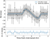 |
Fig. E1 Same as Fig. 1 for WASP-59b. |
| In the text | |
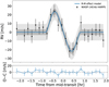 |
Fig. E2 Same as Fig. 1 for WASP-140 Ab with HARPS. |
| In the text | |
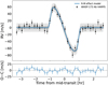 |
Fig. E3 Same as Fig. 1 for WASP-173 Ab with HARPS. |
| In the text | |
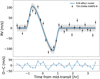 |
Fig. E4 Same as Fig. 1 for TOI-2046b. |
| In the text | |
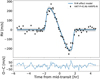 |
Fig. E5 Same as Fig. 1 for HAT-P-41 Ab. |
| In the text | |
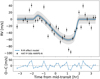 |
Fig. E6 Same as Fig. 1 for HAT-P-50b. |
| In the text | |
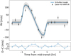 |
Fig. E7 Same as Fig. 1 for Qatar-4b. |
| In the text | |
Current usage metrics show cumulative count of Article Views (full-text article views including HTML views, PDF and ePub downloads, according to the available data) and Abstracts Views on Vision4Press platform.
Data correspond to usage on the plateform after 2015. The current usage metrics is available 48-96 hours after online publication and is updated daily on week days.
Initial download of the metrics may take a while.