| Issue |
A&A
Volume 679, November 2023
|
|
|---|---|---|
| Article Number | A70 | |
| Number of page(s) | 17 | |
| Section | Planets and planetary systems | |
| DOI | https://doi.org/10.1051/0004-6361/202244940 | |
| Published online | 08 November 2023 | |
TOI-858 B b: A hot Jupiter on a polar orbit in a loose binary★,★★
1
Départment d’astronomie de l’Université de Genève,
Chemin Pegasi 51,
1290
Versoix, Switzerland
e-mail: This email address is being protected from spambots. You need JavaScript enabled to view it.
2
European Southern Observatory,
Karl-Schwarzschild-Straße 2,
85748
Garching bei München, Germany
3
Steward Observatory, University of Arizona,
933 North Cherry Avenue,
Tucson, AZ
85721, USA
4
Department of Astrophysical Sciences, Princeton University,
4 Ivy Ln,
Princeton, NJ
08544, USA
5
Cahill Center for Astrophysics, California Institute of Technology,
1216 East California Boulevard,
Pasadena, CA
91125, USA
6
Cerro Tololo Inter-American Observatory,
Casilla 603,
La Serena, Chile
7
Center for Astrophysics – Harvard & Smithsonian,
60 Garden Street,
Cambridge, MA
02138, USA
8
Department of Astronomy, Yale University,
266 Whitney Avenue,
New Haven, CT
06511, USA
9
El Sauce Observatory, Río Hurtado,
Coquimbo Province, Chile
10
Bryant Space Science Center, Department of Astronomy, University of Florida,
Gainesville, FL
32611, USA
11
Astrophysics Group, Keele University,
Staffordshire
ST5 5BG, UK
12
European Southern Observatory,
Alonso de Córdova 3107, Vitacura, Casilla
19001,
Santiago, Chile
13
Department of Physics and Astronomy, The University of North Carolina at Chapel Hill,
120 E. Cameron Ave., Phillips Hall CB3255,
Chapel Hill, NC
27599-3255, USA
14
Brierfield Observatory,
Bowral NSW
2576, Australia
15
Space Telescope Science Institute,
3700 San Martin Drive,
Baltimore, MD
21218, USA
16
Department of Earth, Atmospheric, and Planetary Sciences, Massachusetts Institute of Technology,
77 Massachusetts Avenue,
Cambridge, MA
02139, USA
17
Department of Physics and Kavli Institute for Astrophysics and Space Research, Massachusetts Institute of Technology,
77 Massachusetts Avenue,
Cambridge, MA
02139, USA
18
Department of Aeronautics and Astronautics, Massachusetts Institute of Technology,
77 Massachusetts Avenue,
Cambridge, MA
02139, USA
19
Department of Physics and Astronomy, Vanderbilt University,
PMB 401807,
2301 Vanderbilt Place,
Nashville, TN
37235, USA
20
Hazelwood Observatory,
Victoria, Australia
21
Department of Astronomy, Indiana University,
727 East 3rd Street, Swain West 318,
Bloomington, IN
47405, USA
22
Dunlap Institute for Astronomy and Astrophysics, University of Toronto,
50 St. George Street, Toronto,
Ontario
M5S 3H4, Canada
Received:
9
September
2022
Accepted:
17
August
2023
Abstract
We report the discovery of a hot Jupiter on a 3.28-day orbit around a 1.08 M⊙ G0 star that is the secondary component in a loose binary system. Based on follow-up radial velocity observations of TOI-858 B with CORALIE on the Swiss 1.2 m telescope and CHIRON on the 1.5 m telescope at the Cerro Tololo Inter-American Observatory (CTIO), we measured the planet mass to be 1.10−0.07+0.08 MJ. Two transits were further observed with CORALIE to determine the alignment of TOI-858 B b with respect to its host star. Analysis of the Rossiter-McLaughlin signal from the planet shows that the sky-projected obliquity is λ = 99.3−3.7+3.8°. Numerical simulations show that the neighbour star TOI-858 A is too distant to have trapped the planet in a Kozai–Lidov resonance, suggesting a different dynamical evolution or a primordial origin to explain this misalignment. The 1.15 M⊙ primary F9 star of the system (TYC 8501-01597-1, at ρ ~11″) was also observed with CORALIE in order to provide upper limits for the presence of aplanetary companion orbiting that star.
Key words: planets and satellites: detection / planets and satellites: individual: TOI-858B / planets and satellites: individual: TOI-858A / planets and satellites: dynamical evolution and stability / binaries: visual
Tables A.1–A.3 are available at the CDS via anonymous ftp to cdsarc.cds.unistra.fr (130.79.128.5) or via https://cdsarc.cds.unistra.fr/viz-bin/cat/J/A+A/679/A70
Based on observations collected at the European Southern Observatory, Chile with the CORALIE echelle spectrograph mounted on the 1.2 m Swiss telescope at La Silla Observatory and with ESO HARPS Open Time (123.C-0123, 123.C-0123).
© The Authors 2023
 Open Access article, published by EDP Sciences, under the terms of the Creative Commons Attribution License (https://creativecommons.org/licenses/by/4.0), which permits unrestricted use, distribution, and reproduction in any medium, provided the original work is properly cited.
This article is published in open access under the Subscribe to Open model. This email address is being protected from spambots. You need JavaScript enabled to view it. to support open access publication.
1 Introduction
The thousands of exoplanets that have already been discovered show not only a wide variety in size, density, interior, and atmospheric structure but also in orbital configuration. With every survey based on new or improved detection and characterisation techniques, this variety grows (see reviews in Udry & Santos 2007; Bowler 2016; Zhu & Dong 2021, and references therein).
Such surveys have made it possible to highlight the strong connection between a host star’s properties and those of its orbiting planets, which are often directly linked to their formation history, such as metallicity favouring giant planet formation (e.g., Santos et al. 2004; Fischer & Valenti 2005). These surveys also revealed that small-planet occurrence is not affected by the stellar host properties (Sousa et al. 2008; Buchhave et al. 2012) or the fact that late type stars tend to host smaller planets (Bonfils et al. 2013; Mulders et al. 2015).
Another important link has been shown with the presence of a stellar companion, such as the suppression of planet formation in close binaries, with a limit found to be at 47 au or 58 au by Kraus et al. (2016) and Ziegler et al. (2021), respectively. Indeed, Hirsch et al. (2021) reported a strong drop in planet occurrence rate at binary separations of 100 au, with planet occurrence rates of ~20% for binary separations larger than 100 au and of 4% within 100 au. Moreover, an overabundance, by a factor of about three, of hot Jupiters has also been noted when a stellar companion was found (Law et al. 2014; Ngo et al. 2016; Wang et al. 2017), as well as an increase in eccentricities (Moutou et al. 2017). To a wider extent, Fontanive & Bardalez Gagliuffi (2021) have shown that the influence of a stellar companion is strongest for high mass planets and short orbital periods. However, these demographic results are mainly inferred from the planetary parameters accessible through transit and radial velocity (RV) observations, such as the orbital periods, masses, radii, eccentricities, stellar host properties, and dynamics in the case of systems with multiple planets and even multiple stars.
An important additional parameter that is difficult to obtain is the orbital obliquity, or spin-orbit angle, which is the angle between the stellar spin axis and the axis of the orbital plane. Various approaches have been developed to measure it, namely, the analysis of disc-integrated RVs (Queloz et al. 2010), Doppler tomography (Collier Cameron et al. 2010), and the reloaded Rossiter-McLaughlin effect (Rossiter 1924; McLaughlin 1924; Cegla et al. 2016), which requires performing high-resolution spectroscopy during a planet’s transit.
The spin-orbit angle is a tracer of a planet’s history, shedding light on its formation and evolution (see reviews by Triaud 2018 and Albrecht et al. 2022). Measuring the spin-orbit angle can help one distinguish between a smooth dynamical history that keeps the system aligned, such as migration within the protoplanetary disc (e.g., Winn & Fabrycky 2015), and more disruptive scenarios in which the planetary orbit is tilted through gravitational interactions with the star or with outer companions (e.g., Fabrycky & Tremaine 2007, Teyssandier et al. 2013). Misaligned spin-orbit angles can have either a primordial (i.e., occurring during the star-planet formation) or a post-formation origin (taking place after disc dispersal). Primordial mechanisms, such as magnetic warping or chaotic accretion, tend to produce mild misalignments (Albrecht et al. 2022), unless a distant stellar companion exists, which can either enhance the magnetic warping of the inner disc (Foucart & Lai 2011) or gravitationally tilt the disc (Batygin 2012). While the latter process has recently been disfavoured due to planet-star coupling damping the effect (Zanazzi & Lai 2018), the magnetic warping aided by a stellar companion could lead to a large distribution of obliquities, including retrograde planets (Foucart & Lai 2011). Post-formation misalignments are driven by gravitational interactions involving a third body (planet or star). While planet-planet scattering can produce misalignments of up to 60 degrees (Chatterjee et al. 2008), a close encounter with another star would yield an isotropic distribution of obliquities, although this process is only expected in a very dense cluster environment (Hamers & Tremaine 2017). The post-formation gravitational interactions can also lead to high-eccentricity tidal migration, where a planet that is originally far from its central star acquires high eccentricity, and its orbit is later circularised (and shrunk) due to the strong stellar tides suffered near periastron. In this process, the driver of the increase in eccentricity is the Kozai–Lidov effect induced by a third massive external companion, such as a star or a brown dwarf (Kozai 1962). This mechanism has been proposed as a source of hot Jupiters (Dawson & Johnson 2018) and can also lead to spin-orbit misalignment (Fabrycky & Tremaine 2007). Recently, Vick et al. (2023) showed that if the system already has a primordial misalignment (from companion-disc interaction, stellar spin-disc interaction, and disc dispersal), Kozai–Lidov oscillations lead to predominantly retrograde stellar obliquities, with the distribution of angles peaking at a misalignment of around 90 degrees (i.e., polar orbits) for hot Jupiters.
In this work, we focused our exoplanet search around the wide stellar binary system TOI-858 A-B, which has an angular separation of ρ ~ 11″ (~3000 au; Gaia Collaboration 2021). Wide binaries (i.e., binary separations in the range of 300–20 000 au) are common in our galaxy (Offner et al. 2023), yet their origin remains a mystery because they easily become disrupted in dense star-forming regions (Offner et al. 2023). The most accepted formation channel for wide binaries is during the phase of star cluster dissolution (Kouwenhoven et al. 2010; Moeckel & Bate 2010).
In this study, we apply the latest Rossiter-McLaughlin technique (i.e., Revolutions, or RMR; Bourrier et al. 2021) to two transits of TOI-858 B b observed with the CORALIE spectrograph on the 1.2 m Swiss telescope at La Silla Observatory (Sect. 4.1) in order to measure the spin-orbit angle between TOI-858 B b and TOI-858 B. The paper is structured as follows. We first describe the discovery and follow-up observations of the 1.08 M⊙ G0 (Pecaut & Mamajek 2013) star TOI-858 B and its nearby and similarly bright (ΔmagTESS = 0.248) 1.15 M⊙ F9 stellar companion TOI-858 A (Sect. 2). Then, we present the joint analysis of the acquired data leading to the confirmation of the planet (Sect. 3). Further investigation of the orbital architecture of the TOI-858 B system along with the link to the nearby star TOI-858 A is given in Sect. 4. Finally, the results are discussed in Sect. 5.
2 Observations
A summary of the photometry and high-resolution spectroscopy data used in the joint analysis of TOI-858 B b can be found in Tables 1 and 2. Additionally, SOAR speckle imaging was used to rule out nearby stellar companions, as described in Sect. 2.5.
2.1 TESS discovery photometry
The star TOI-858 B (TIC 198008005) was observed by the Transiting Exoplanet Survey Satellite (TESS; Ricker et al. 2015) in Camera 3 in sectors 3, 4, 29, 30, and 31. For the first two sectors, 30-min cadence full-frame images (FFIs) are available. TOI-858 B b was identified as a TESS Object of Interest (TOI) based on the MIT Quick Look Pipeline data products (QLP; Huang et al. 2020a,b). In our joint analysis, for sectors 3 and 4, we used the extracted photometry from the QLP pipeline. During the third year of the TESS mission, TOI-858 B was observed with a 2-min cadence in sectors 29, 30, and 31. The light curves used in our joint analysis from these sectors are publicly available at the Simple Aperture Photometry flux with Pre-search Data Conditioning (PDC-SAP; Stumpe et al. 2014, 2012; Smith et al. 2012; Jenkins et al. 2010) provided by the Science Processing Operations Center (SPOC; Jenkins et al. 2016).
Within the large 21″ TESS pixels, TOI-858 B is completely blended with a slightly brighter star, TOI-858 A (TIC-198008002). The two sources are separated by 10.7″. Based on the TESS data alone, it is not possible to determine around which of the two stars the transits are taking place. A combination of seeing-limited ground-based photometry and RV measurements helped determine which of the two stars host the planet (discussed in Sect. 2.2 and 2.4).
Summary of the discovery TESS photometry, archival WASP-South photometry, and ground-based follow-up photometry of TOI-858 B.
Summary of the RV observations of TOI-858 B.
2.2 Ground-based follow-up photometry
The TESS pixel scale is ~21″ pixel−1, and photometric apertures typically extend out to roughly 1 arcmin, generally causing multiple stars to blend in the TESS photometric aperture. To determine the true source of the TESS detection, we acquired ground-based time-series follow-up photometry of the field around TOI-858 B as part of the TESS Follow-up Observing Program (TFOP; Collins et al. 2018)1. The follow-up light curves were also used to confirm the transit depth and thus the TESS photometric de-blending factor as well as to refine the TESS ephemeris and place constraints on transit depth differences across optical filter bands. We used the TESS Transit Finder, which is a customised version of the Tapir software package (Jensen 2013), to schedule our transit observations. The photometric data were extracted using the AstroImageJ (AIJ) software package (Collins et al. 2017). The observations are summarised in the following subsections and in Table 3. As shown in Fig. 1, they confirm that the TESS-detected transit-like event is occurring around TOI-858 B.
2.2.1 Hazelwood Observatory
We observed an ingress of TOI-858 B b in Sloan i′-band on UTC 2019 August 28 from Hazelwood Observatory near Churchill, Victoria, Australia. The 0.32 m telescope is equipped with a 2184 × 1472 SBIG STT3200 camera. The image scale is (0″.55 pixel−1, resulting in a 20′ × 14′ field of view. The photometric data were extracted using a circular 5″.9 photometric aperture.
2.2.2 Brierfield Observatory
We observed a full transit in B-band on UTC 2019 November 5 from Brierfield Observatory near Bellingen, New South Wales, Australia. The 0.36 m telescope is equipped with a 4096 × 4096 Moravian 16803 camera. The image scale after binning 2×2 is 1″.47 pixel−1, resulting in a 50′ × 50′ field of view. The photometric data were extracted using a circular 4″.4 photometric aperture.
2.2.3 Evans 0.36 m Telescope
We observed a full transit in B-band on UTC 2019 December 5 from the Evans 0.36 m telescope at El Sauce Observatory in Coquimbo Province, Chile. The telescope is equipped with a 1536 × 1024 SBIG STT-1603-3 camera. The image scale after binning 2×2 is 1″.47 pixel−1, resulting in an 18.8′ × 12.5′ field of view. The photometric data were extracted using a circular 5″.9 photometric aperture.
2.3 WASP-South archival photometry
The TOI-858 B system was observed in 2010 and 2011 by the WASP-South survey when it was equipped with 200-mm, f/1.8 lenses observing with a 400–700 nm passband (Pollacco et al. 2006). The 48-arcsec extraction aperture encompasses both stars of the binary. A total of 6445 photometric data points were obtained, spanning 110 nights starting in 2010 August and then another 170 nights starting 2011 August. The standard WASP transit-search algorithms (Collier Cameron et al. 2006) detect the 3.27-day periodicity (though the object was never selected as a WASP candidate) and report an ephemeris of JD(TDB) = 245 5982.41565(13) + E × 3.279765(13).
TFOP photometric follow-up observation log.
2.4 High-resolution follow-up spectroscopy
The high-resolution spectrographs CORALIE, HARPS, and CHIRON were utilised to fully characterise the TOI-858 B system. Multi-epoch monitoring allowed us to measure the reflex motion of the star(s) induced by the planet. Furthermore, we observed two spectroscopic transits of TOI-858 B b with the aim of determining the spin-orbit angle of TOI-858 B b.
2.4.1 CORALIE
Both TOI-858 B and TOI-858 A were observed with the CORALIE spectrograph mounted on the Swiss 1.2 m Euler telescope at La Silla Observatory, Chile (Queloz et al. 2001b). CORALIE has a resolution of R = 60 000 and is fed by a 2″ on-sky A fibre. An additional B fibre can be used to either provide simultaneous Fabry-Pérot (FP) RV drift monitoring or on-sky monitoring of the background contamination.
We obtained 22 spectra between 2019 August13 and 2021 January 18 UT with simultaneous FP to monitor the RV of TOI-858 B as it was orbited by TOI-858 B b. The exposure times ranged between 1800 and 1200 s, depending on the observing schedule, resulting in an average S/N per pixel of 15 at 5500 Å.
Two spectroscopic transits were also observed on 2019 December 5 and 2021 January 18 UT. On both nights, we obtained 11 spectra with individual exposure times of 1800s. During the first visit (2019-12-05) one spectrum was obtained before transit, seven spectra during transit, and three after transit. We observed without any simultaneous wavelength calibration in order to enable correction for sky contamination monitored with the B fibre. In this mode, the wavelength solution originates from the calibration acquired during daytime. Instrumental drift during the night is not taken into account but were expected to be smaller than or on-par with the expected RV uncertainty for this target. After receiving ambiguous results, we repeated the observations on the second night (2021-01-18) with simultaneous FP. During this visit, we took one spectrum before transit, six spectra during transit, and four after transit.
For TOI-858 A, we acquired nine CORALIE spectra between 2019 October 17 and 2020 March 12 UT in order to check for additional stars and giant planets in the system. All spectra were taken with simultaneous FP, and nearly all had exposure times of 1800 s, while one was set to 1200 s. The average S/N per pixel were 19 at 5500 Å.
All spectra were reduced with the standard CORALIE Data Reduction Software (DRS). Spectra for both stars were cross-correlated with a G2 binary mask (Baranne et al. 1996) to extract RV measurements as well as cross-correlation function (CCF) line diagnostics, such as bisector-span (Queloz et al. 2001a) and full width at half maximum (FWHM). We also derived H-α activity indicators for each spectrum. Two spectra taken on 2019 September 29 and 2019 September 30 UT were rejected by the automatic quality control of the DRS due to a large instrument drift of more than 150 m s−1, which can lead to less precise drift correction of a few m s−1. For the analysis of TOI-858 B b, we deemed these drift-corrected RVs to still be useful, as the obtained RV uncertainties are larger than the error on the drift correction. Furthermore, the measured RV semi-amplitude is more than 100 m s−1 (Tables A.1 and A.3).
2.4.2 HARPS
With the HARPS spectrograph on the 3.6 m ESO telescope at the La Silla Observatory, Chile (Pepe et al. 2002b), half a spectroscopic transit was observed on 2019 December 5. This took place during technical time, when the new HARPS+NIRPS front end (Bouchy et al. 2017) was being commissioned. In total, six spectra were obtained in high efficiency mode (EGGS), which trades spectral resolution for up to twice the throughput by using a slightly larger on-sky fibre (1.4 ″) than the high accuracy mode (HAM, 1″) but is still small enough to prevent contamination from the secondary star. The first two spectra have exposure times of 900 s, which was then decreased to 600 s to get a better time resolution during transit. The spectra have S/N 40−30 per pixel at 5500 Å, and RV uncertainties of 3.5–5 m s−1. Only one spectrum was taken out of transit.
All HARPS spectra were reduced with the offline HARPS DRS hosted at the Geneva Observatory. Using a sufficiently wide velocity window of 60 km s−1, CCFs were derived with a G2 binary mask.
2.4.3 CHIRON
We obtained spectroscopic data of TOI-858 B using the CHIRON spectrograph (Tokovinin et al. 2013), a high-resolution fibre-fed spectrograph mounted on the 1.5 m telescope at the Cerro Tololo Inter-American Observatory (CTIO) in Chile. We obtained in total seven different spectra between 2019 August 9 and 2019 September 1. For these observations, we used the image slicer mode (resolving power ~80 000) and an exposure time of 600 s, leading to a relatively low S/N per pixel of ~8– 10 at 5500 Å and RV uncertainties of 20–40 m s−1. In addition, a ThAr lamp was taken before each observation, from which a new wavelength solution was computed. The data were reduced using the Yale pipeline, and the RVs were computed following the method described in Jones et al. (2019), which has shown a long-term RV precision on τ Ceti of ~ 10–15 m s−1. We note that our method computes relative RVs with respect to a template that is built by stacking all of the individual spectra. Therefore, the systemic velocity is not included in the final RVs, which explains the large offset between the CHIRON and CORALIE velocities. The Barycentric Julian Date (BJD), RV, and the corresponding 1σ RV uncertainties are listed in Table A.2.
2.5 Speckle imaging
Additional nearby companion stars not previously detected in seeing-limited imaging can result in photometric contamination, reducing the apparent transit depth. We searched for nearby sources of TOI-858 B with SOAR speckle imaging (Tokovinin 2018) on 2019 August 8 UT in I-band, a visible bandpass similar to TESS. Further details of the observations from the SOAR TES S survey are available in Ziegler et al. (2020). We detected no nearby stars within 3″of TOI-858 B within the 5σ detection sensitivity of the observation, which is plotted along with the speckle auto-correlation function (ACF) in Fig. 2.
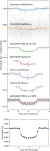 |
Fig. 1 Photometric transit observations of TOI-858 B b in 20 min bins. The vertical dashed lines represent meridian flips. The bottom panel shows all light curves phase folded and overplotted. |
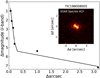 |
Fig. 2 SOAR speckle imaging in Cousins I-band excluding nearby stars down to A Imag ~5 within 3″ of TOI-858 B. The inset is the speckle ACF centred on the target star. |
3 Analysis
3.1 Spectral analysis
Stellar atmospheric parameters for TOI-858 B and TOI-858 A were derived using SPECMATCH-EMP (Yee et al. 2017). For TOI-858 B, we stacked the six HARPS-EGGS spectra to get one high-fidelity spectrum for the analysis, and for TOI-858 A, we ran SPECMATCH-EMP on the stacked spectrum created from nine CORALIE spectra.
The SPECMATCH-EMP tool matches the input spectrum to a large spectral library of stars with well-determined parameters that have been derived with interferometry, optical and near-infrared (NIR) photometry, asteroseismology, and local thermodynamic equilibrium (LTE) analysis of high-resolution optical spectra. The wavelength range encompassing the Mg I b triplet (5100–5340 Å) was utilised to match our spectra to the built-in SPECMATCH-EMP spectral library through χ2 minimisation. A weighted linear combination of the five best matching spectra were used to extract Teff, Rs, and [Fe/H]. For TOI-858 B, we obtained Teff of 5948 + 110 K, Rs = 1.27 + 0.18R⊙, and [Fe/H] = 0.17 + 0.09 (dex). For TOI-858 A, the spectral analysis yielded Teff = 5911 + 110 K, Rs = 1.47 + 0.18R⊙, and [Fe/H]= 0.21 + 0.09 (dex). The Teff and [Fe/H] were used as priors in the joint analysis detailed in Sects. 3.3 and 3.4, which models the system using broadband photometry, Gaia information, stellar evolutionary models, and (when available) transit light curves. The final stellar parameters are listed in Tables 4 and 5.
3.2 Stellar rotation
The projected rotational velocity, v sin i, was computed for each star using the calibration between v sin i and the width of the CORALIE CCF. This calibration was first presented in Santos et al. (2002), and it has since been updated as CORALIE has undergone several updates (Raimbault 2020). For TOI-858 B, we obtained v sin i = 5.80 ± 0.25 km s−1, and for TOI-858 A, we obtained υ sin i = 6.40 ± 0.25 km s−1. Using the stellar radii listed in Tables 6 and 5, the projected rotational velocities correspond to Prot/ sin i of 11.5 ± 0.7 days and 10.8 ± 0.7 days, respectively.
We observed clear rotational modulation in both the TESS and WASP-South light curves. From top to bottom, Fig. 3 shows the Lomb–Scargle periodograms computed for the WASP-South data before and after the change to the 85 mm lenses in 2010 and 2011, the TESS QLP light curve without de-trending (SAP), and the SPOC-de-trended (PDCSAP) light curve. The transits of TOI-858 B b were masked to avoid picking up the planetary signal. A clear and persistent modulation can be seen at a period of 6.2–6.4 days in both the WASP-South and TESS data, having an amplitude varying between 2 and 3 mmags. The TESS light curves cover only a few stellar rotations, whereas the two WASP-South data sets each cover multiple seasons.
Using the WASP-South data only and a modified Lomb-Scargle periodogram approach that is tailored to the noise characteristics of WASP data, as discussed in Maxted et al. (2011), we found a rotation period of Prot = 6.42 ± 0.10 days. Since TOI-858 B and TOI-858 A are fully blended in both WASP-South and TESS, we could not determine which of the stars is responsible for the rotational modulation. There are no signs of two distinct rotational signals in the photometry nor at the Prot/ sin i derived from the CORALIE CCFs. For TOI-858 B, an inclination of 34° is needed to align the Prot measured from the light curves with the spectroscopic Prot/ sin i, and for TOI-858 A, it is 36°.
For Prot = 6.42 ± 0.02 days, gyro-chronology yields an age of 0.3–0.4 Gyr (Barnes 2007) for either of the two stars. This is not in agreement with the ages derived in Sect. 3.3 based on a spectral energy distribution (SED) fitting with the Mesa Isochrones and Stellar Tracks (MIST) evolutionary models. Moreover, following the approach described in Bouma et al. (2021), we found no sign of Li absorption in the high S/N stacked spectra for either star, which could otherwise support a hypothesis of a young age. The discrepancy between the stellar age derived with gyro-chronology and MIST could indicate that the planet-hosting star TOI-858 B has been spun-up by the planet, as such is the case for HAT-P-llb (Bakos et al. 2010), which shows evidence of tidal spin and high stellar activity (Morris et al. 2017; Tejada Arevalo et al. 2021). We note that the rotation period of 6.42 + 0.02 days is close to twice the planetary orbital period, Pb = 3.28 days. The similar usin; measured for the two stars could in this case be explained by differences in inclination.
Stellar properties for TOI-858 B.
Stellar parameters for TOI-858 A.
Median values and 68% confidence intervals for the TOI-858 B system.
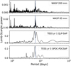 |
Fig. 3 Periodograms showing the stellar rotational modulation in the WASP-South and TESS data, spanning 11 years in total. All data sets indicate a rotation period of 6.4−6.2 days. The vertical blue lines in all four panels indicate Prot = 6.42 days, determined using the WASP-South data (200 mm and 85 mm). |
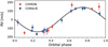 |
Fig. 4 Phase folded CORALIE and CHIRON RV measurements for TOI-858 B. |
3.3 Joint modelling of radial velocities and transit light curves
The TESS photometry, ground-based follow-up transit photometry, WASP-South archival light curves, and RV measurements from CORALIE and CHIRON were jointly modelled using EXOFASTv2 (Eastman et al. 2013, 2019). In this approach, both stellar and planetary parameters are derived for any number of transits and RV instruments while exploring the large parameter space through a differential evolution Markov chain and Metropolis-Hastings Monte Carlo sampler (MCMC).
The transit model is based on the analytical expressions in Mandel & Agol (2002), and the RVs are modelled as a classic Keplerian orbit. The planet properties are described by seven free parameters: RV semi-amplitude (K), planet radius (Rp), orbital inclination (i), orbital period (P), time of conjunction (TC), eccentricity (e), and argument of periastron (ω*). Two additional RV terms, systemic velocity and RV jitter, are also fitted for each instrument (CORALIE & CHIRON). Because the CHIRON RVs are derived with respect to a median spectral template, the systemic velocity for the instrument is therefore close to zero (Fig. 4).
For the transit light curves, a set of two limb-darkening coefficients for each photometric band were evaluated by interpolating tables from Claret & Bloemen (2011); Claret (2017). This was done within EXOFASTv2 at each MCMC step. The limb-darkening coefficients are fitted along with the out-of-transit baseline flux and variance. The WASP-South data were heavily blended, with more than 50% of the flux in the aperture coming from TOI-858 A. To take this into account, we fitted a dilution parameter to the WASP-South light curves. A Gaussian prior on the dilution factor, based on the Gaia GRP magnitudes of the two stars, was imposed. Similarly, we also included a dilution term for the TESS data to take imperfect de-blending into account and to propagate the error that might come with it. The light curves from Hazelwood and Brierfield include meridian flips, indicated by the dashed lines in Fig. 1. Any offset between the data obtained before and after a meridian flip was modelled as a multiplicative de-trending term that multiplies the flux after the meridian flip with a constant. Furthermore, the El Sauce light curve was multiplicatively de-trended with airmass within EXOFASTv2. The Brierfield time series was likewise detrended against total flux counts. (For more information on the de-trending, see Sect. 11 of Eastman et al. 2019.)
Along with the planetary properties, the stellar parameters were also modelled at each step in the MCMC. This allowed us to utilise the information on transit duration and orbital eccentricity embedded in the transit light curves and RVs to constrain the stellar density (Seager & Mallén-Ornelas 2003; Kipping et al. 2012; Eastman et al. 2023). We imposed Gaussian priors on Teff and [Fe/H] from the spectral analysis presented in Sect. 3.1 while fitting the SED based on archival broadband photometry presented in Table 4. When including the Gaia DR3 parallax as a Gaussian prior, we obtained a tight constraint on the stellar radius. We also included an upper limit on the V-band extinction from Schlegel et al. (1998) and Schlafly & Finkbeiner (2011) to constrain line-of-sight reddening. Table 7 lists the informative priors described in this section and summarises the values applied. To improve the stellar mass we obtained from combining the stellar radius with the stellar density from the transit light curve, we queried the MIST models (Dotter 2016; Choi et al. 2016). This meant comparing the fitted stellar model parameters to viable MIST values at each step of the MCMC. The joint model was penalised for the difference between the two. This method uses MIST to guide the stellar parameters rather than to define them and can help break degeneracies encountered when using only isochrone models. Despite EXO-FASTv2 having the ability to include Doppler tomography and the Rossiter-McLaughlin effect in its joint model, we found that a more sophisticated analysis of the spectroscopic transit data was needed, as outlined in the Sect. 4.1.
Informative priors invoked in the EXOFASTv2 model for the TOI-858 B system.
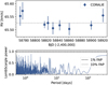 |
Fig. 5 CORALIE RV measurements of TOI-858 A. Top panel: RV time series showing no clear signs of a giant planet in a short period orbit. Lower panel: Lomb–Scargle periodogram for the RVs with no significant signals detected. The false alarm probability (FAP) levels of 1% and 10% are indicated as horizontal lines. |
3.4 Stellar properties of TOI-858A
We derived stellar parameters for TOI-858 A in a similar way as outlined for TOI-858 B in Sect. 3.3, using EXOFASTv2 to perform an SED fit combined with MIST, while no additional information on stellar density from a transit light curve was available. We used Gaussian priors on Teff = 5911 ± 110 K, [Fe/H] = 0.21 ± 0.09 (dex) and parallax of 4.0181 ± 0.0146 (mas). For the V-band extinction, an upper limit from dust maps of 0.04 mag was used. The final stellar properties of TOI-858 A are listed in Table 5. The ages we got for TOI-858 B and TOI-858 A are in agreement with each other, though poorly constrained.
The CORALIE RVs of TOI-858 A showed no sign of planets, though only giant planets in relatively short period orbits could be ruled out. Figure 5 shows the RV time series with a generalised Lomb–Scargle periodogram at the bottom. No periodic signals were detected down to a false alarm probability of 10%. We found the systemic velocity of TOI-858 A measured with CORALIE to be 65.523 ± 0.006 km s−1, which is in agreement with the Gaia EDR3 RV of 65.5 ± 0.6 km s−1 and similar to the 64.7 ± 0.7 km s−1 of TOI-858 B found by Gaia (Gaia Collaboration 2021).
4 Analysis of TOI-858 B orbital architecture
We further investigated the orbital architecture of the TOI-858 B, TOI-858 B b, and TOI-858 A ensemble. To carry out this study, we characterised the planet orbit through a Rossiter-McLaughlin observation (described in Sect. 4.1), and we analysed the link between the two stars and their possible impact on the planet orbit (Sect. 4.2).
4.1 Rossiter-McLaughlin Revolutions analysis
4.1.1 Transit observations
We utilised the two data sets obtained with CORALIE during the transit of TOI-858 Bb on 2019 December 5 (Visit 1) and 2021 January 18 (Visit 2). Spectra were extracted from the detector images and corrected and calibrated by version 3.8 of the DRS (Baranne et al. 1996; Queloz et al. 1999; Bouchy et al. 2001) pipeline. One of the corrections concerns the colour effect caused by the variability of extinction induced by Earth’s atmosphere (e.g., Bourrier & Hébrard 2014; Bourrier et al. 2018; Wehbe et al. 2020). The flux balance of the TOI-858 B spectra was reset to a Kl stellar spectrum template before the spectra were passed through weighted cross-correlation (Baranne et al. 1996; Pepe et al. 2002a) with a G2 numerical mask to compute the CCFs. Since the CCFs are oversampled by the DRS with a step of 0.5 km s−1, for a pixel width of about 1.7 km s−1, we kept one in three points in all CCFs prior to their analysis. We analysed the two CORALIE visits using the RMR technique, which follows three successive steps that are described hereafter (a full description can be found in Bourrier et al. 2021).
4.1.2 Extraction of the planet-occulted CCFs
In the first step of the RMR technique, the disc-integrated CCFDI were aligned by shifting their velocity table with the Keplerian motion of the star, as calculated using the median values for the stellar and planet properties from the joint fit analysis done in EXOFASTv2, as given in Table 6. The continuum of the CCFDI was then scaled to the same flux outside of the transit and to the flux simulated during transit with the batman package (Kreidberg 2015). The transit depth was taken from Table 6, and limb-darkening coefficients were calculated with the EXOFAST calculator (Eastman et al. 2013) for the stellar properties listed in Table 6. This yielded u1 = 0.45 and u2 = 0.27 in the visible band, representative of the CORALIE spectral range. The CCFDI outside of the transits were co-added to build master-out CCFs representative of the unocculted star. Gaussian profiles were fitted to the master-out CCFDI to determine the RV zero points in Visit 1 (64.353+0.015 km s−1) and Visit 2 (64.358+0.013 km s−1), which were then used to shift all CCFDI to the star rest frame. The CCFs from the planet-occulted regions were retrieved by subtracting the scaled CCFDI from their corresponding master-out. They were finally normalised to a common flux level by dividing their continuum with the flux scaling applied to the CCFDI, yielding intrinsic CCFintr that directly trace variations in the local stellar line profiles (Fig. 6). Flux errors were assigned to the CCFintr as the standard deviation in their continuum flux.
4.1.3 Analysis of individual exposures
In the second step, a Gaussian profile was fitted to the CCFintr in each exposure, over [−30, 30] km s−1 in the star rest frame. We sampled the posterior distributions of its RV centroid, FWHM, and contrast using emcee MCMC (Foreman-Mackey et al. 2013). We set uniform priors on the RV centroid with a boundary between −5 to 10 km s−1, on the FWHM with a boundary between 0 and 20 km s−1, and on the contrast (bounded between −2 and 2). One hundred walkers were run for 2000 steps, with a burn-in phase of 500 steps, to ensure that the resulting chains converged and are well mixed.
As shown in Fig. 6, the stellar line is clearly detected in most individual CCFintr with narrow and well-defined posterior distribution functions (PDFs) for their model parameters (Figs. B.2 and B.3), which allowed us to extract the time series of the local stellar line properties (Fig. 7). The only exception is the first exposure in Visit 2, which was excluded from further analysis. Surprisingly, the local RV series displays larger values overall in Visit 1 than in Visit 2. Nonetheless, both series are positive and constant at the first order, showing that TOI-858 B b transits the stellar hemisphere, rotating away from the observer at about the same stellar longitude. There is no evidence for centre-to-limb variations in the local stellar line shape, as the local contrast and FWHM series remain roughly constant along the transit chord. The width of the local line, however, appears to be broader in the second visit, suggesting a possible change in the stellar surface properties.
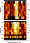 |
Fig. 6 Maps of the CCFintr during the transit of TOI-858 B b in Visit 1 (upper panel) and Visit 2 (lower panel). Transit contacts are shown as green horizontal dashed lines. Values are coloured as a function of their normalised flux and plotted as a function of RV in the stellar rest frame (in abscissa) and orbital phase (in ordinate). The stellar lines from the planet-occulted regions are clearly visible in both visits. The green solid lines show the best-fit model for the stellar surface RVs derived from a joint RMR fit to both data sets. The green vertical dashed lines show the spectroscopic, sky-projected stellar rotational velocity. |
4.1.4 Joint transit analysis
In the third step, all CCFintr were fitted together with a joint model. Based on step two, the local stellar line was modelled as a Gaussian profile with a constant contrast and an FWHM along the transit chord but with values specific to each visit. The RV centroids of the theoretical lines were set by the surface RV model described in Cegla et al. (2016) and Bourrier et al. (2017), assuming solid-body rotation for the stellar photosphere and oversampling each exposure to account for the blur induced by the planet motion (a conservative oversampling factor of five was used). The time series of the theoretical stellar lines were convolved with the CORALIE instrumental response and then fitted to the CCFintr in both visits using emcee MCMC. The model parameters used as jump parameters for the MCMC were the line contrast and FWHM, the sky-projected obliquity λ, and stellar rotational velocity υ sin i*. Uniform priors were set on all parameters: over the same range as in step two for the contrast and FWHM, between [0–30] km s−1 for υ sin i*, and over its definition range ([−180, 180]°) for λ.
Posterior distribution functions for the model parameters are shown in Fig. B.1. The best fit yielded a reduced χ2 of 1.3 (χ2 = 634 for 474 degrees of freedom) with models that reproduce the local stellar lines along the transit chord well, as can be seen in the residual maps shown in Fig. 8. Properties of the best-fit line model convolved with the CORALIE response are shown in Fig. 7. The local line has a similar contrast in the two visits ( for Visit 1 and 74.1+5.2% for Visit 2), but it is significantly broader in the second visit (
 km s−1 for Visit 1 and 10.44+0.75 km s−1 for Visit 2). Whether the origin of this variation is stellar or not, we note that λ and υ sin i* are not correlated with the contrast and FWHM of the fitted lines (Fig. B.1). We derived υ sin i* = 7.09±0.52 km s−1, which is larger than the value of 5.80 ± 0.25 km s−1 obtained from a spectroscopic analysis of the CORALIE data. The main result from our analysis is the derivation of the projected spin–orbit angle,
  , which shows that TOI-858 B b is on a polar orbit.
We performed two tests to assess the reliability of this conclusion. First, as the derived local line contrasts depend on the accuracy of the transit light curve used to scale the CCFDI (Sect. 4.1.2), we thus varied the transit depth of TOI-858 B b within its 3σ uncertainties. We found that it changes λ by less than 0.5°. Then, we fitted the two visits independently. We found significant differences between the derived υ sin i* (8.2±0.6 km s−1 in Visit 1 and 3.6±0.9 km s−1 in Visit 2), neither of which is similar with the value derived from the CORALIE CCF-width in Sect. 3.2 (5.80±0.25 km s−1). Interestingly, the latter is consistent with the weighted mean of Visit 1 and 2 values (6.8±0.5 km s−1). In the present case of a polar orbit, the rotational velocity is directly constrained by the overall level of the surface RV series, which explains why we derived different values for the two visits (Fig. 7). The physical origin of this difference, however, is unclear. No detrimental contamination was identified in Fibre B of CORALIE, which was pointing on-sky in Visit 1. It is possible that an instrumental drift may have biased the RVs during the visit, which is why we put Fibre B on the FP simultaneous reference in Visit 2. The first half of the transit in Visit 2 was obtained with lower S/N (down to 12 in the first exposures compared to 17 afterwards, as measured in order 46), possibly due to a change in sky conditions. This makes it difficult to determine which data set is the most accurate, considering that they mainly differ during the first half of the transit. The projected spin-orbit angle, however, is less affected by these variations than υ sin i* and remains consistent within 1σ between the two visits ( in Visit 1 and
  in Visit 2), confirming the misalignment of the TOI-858 B b orbital plane.
To calculate the actual obliquity (as opposed to its sky projection), we needed information about the inclination of the stellar rotation axis relative to the line of sight. Such information can be obtained from the combination of the stellar radius, rotation period, and projected rotation velocity (υ sin i★). In this case, the rotation period of the planet-hosting star, TOI-858 B, is uncertain. A photometric period of 6.4 days was detected in the TESS and WASP-South light curves, but the period might belong to TOI-858 A instead. Bearing this caveat in mind and assuming the period belongs to B, we derived constraints on the stellar inclination angle using an MCMC procedure, following Masuda & Winn (2020). The free parameters were cos i★, which was subject to a uniform prior; R★/R⊙, which was subject to a Gaussian prior with a mean of 1.308 and standard deviation of 0.038 (see Table 6); and Prot, which was subject to a Gaussian prior with a mean of 6.42 days and a standard deviation of 0.64 days (enlarged to 10% to account for systematic effects such as differential rotation). The log-likelihood was taken to be
 (1)
(1)
based on the CORALIE-based measurement of υ sin i★. The result for cos i★ was  . We combined this result with the measurements of λ = 99.3 + 3.8 degrees and i0 = 86.8 + 0.5 degrees to arrive at two possibilities for the stellar obliquity: ψ = 92.7 + 2.5 degrees or 98.0 + 2.5 degrees (the discrete degeneracy arises because we do not know the relative signs of cos i★ and cos i0). Thus, under these assumptions, the stellar spin axis and normal to the orbital plane are nearly perpendicular (Fig. 9).
This conclusion does not depend strongly on the exact constraints on υ sin i★. For example, if we use the constraint υ sin i★ = 7.09 + 0.52 km s−1, based on the RM analysis, the results for ψ are modified to 94.5 + 3.0 and 98.9 + 3.0 degrees. In fact, because λ is so well constrained, the conclusion that the axes are nearly perpendicular does not even depend strongly on the assumption that the rotation period is 6.4 days. When we repeated the calculation for any choice of rotation period between 0.1 and 11 days, the best-fit value of ψ varied between 87 and 100 degrees.
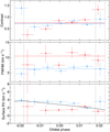 |
Fig. 7 Properties of the stellar surface regions occulted by TOI-858 B b. in blue for Visit 1 and red for Visit 2. The dashed vertical lines are the transit contacts. The horizontal bars indicate the duration of each exposure. The vertical bars indicate the 1σ HDI intervals. The solid curves are the best models to each property, derived from a joint RMR fitted to both visits (excluding the first exposure in Visit 2). The RV model is common to both visits. The model contrast and FWHM are specific to each visit and are shown here after convolution of the model line by the CORALIE line spread function (LSF). |
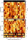 |
Fig. 8 Maps of the out-oſ-transit residuals and of the in-transit residuals between CCFintr and their best-fit model in Visit 1 (top panel) and Visit 2 (bottom panel). Transit contacts are shown as green dashed lines. The green vertical dashed lines show the spectroscopic, sky-projected stellar rotational velocity. |
4.2 Dynamical analysis
4.2.1 The TOI-858 B-TOI-858A system
The two stars, TOI-858 B and TOI-858 A, are separated by ρ ~11″ (~3000 au; Gaia Collaboration 2021) and have similar proper motion and parallax values in Gaia EDR3, suggesting they represent a wide binary pair and are a good target for examination of angular momentum vector alignment between binary and transiting planet orbits. However, the escape velocity for a system of two stars with these given masses and uncertainties at a separation of ~3000 AU is 0.09 + 0.06 km s−1, while the relative velocity vector given by EDR3 proper motions and RV for both stars is 3.8 + 0.2 km s−1, nearly 18-σ higher than the escape velocity. Thus, only unbound, hyperbolic trajectories are consistent with these relative velocities.
Both have high quality EDR3 astrometric solutions as measured by the re-normalised unit weight error (RUWE): TOI-858 B RUWE = 1.009 and TOI-858 A RUWE = 1.0166, where RUWE ≈1 is a well-behaved solution (Lindegren 2018)2. The TOI-858 A–B pair is not resolved in Hipparcos or Tycho. There are two additional astrometric measurements of the pair, both from 1894, in the Washington Double Star Catalogue (WDS; Mason et al. 2001), with ρ = 11.5″ and position angle (PA) = 164° in 1894, compared to ρ = 10.94903 + 1 × 10⁻⁵″, PA = 169.90649 + 6 × 10⁻⁵ deg in Gaia EDR3. The plane-of-sky relative velocity given by those measurements (~ 12 km s−1) is larger than the Gaia EDR3 relative velocity. Neither star is in the El-Badry et al. (2021) catalogue of binaries identified in Gaia EDR3. Following the method described in Pearce et al. (2021, Sect. 3.1.1), we determined the probability of a chance alignment to be ~1 × 10⁻⁶, given the density of all objects in Gaia EDR3 within a 10° radius and 1−σ of the TOI-858 B proper motion and parallax. We conclude that TOI-858 B and TOI-858 A either (1) are a formerly bound binary that recently became unbound, (2) have inaccurate solutions in Gaia EDR3 despite the low RUWE values, or (3) are a chance alignment, despite the low probability. We can thus conclude that the system is either a binary that recently became unbound (conclusion 1) or a binary that has inaccurate Gaia EDR3 solutions (conclusion 2).
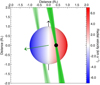 |
Fig. 9 Projection of TOI-858 B in the plane of sky for the best-fit orbital architecture. The black arrow shows the sky-projected stellar spin. The stellar disc is coloured as a function of its surface RV field. The normal to the orbital plane of TOI-858 B b is shown as a green arrow. The thick green solid curve represents the best-fit orbital trajectory. The thin lines surrounding it show orbits obtained for orbital inclination, semi-major axis, and sky-projected obliquity values drawn randomly within 1σ from their probability distributions. The star, planet (black disc), and orbits are to scale. |
4.2.2 Assessment of a Kozai–Lidov evolution
Given the polar orbit of TOI-858 Bb, we examined the possibility of this architecture being caused by the action of the stellar binary companion. Under some circumstances, a distant third body can trigger the Kozai–Lidov effect (Kozai 1962; Lidov 1962; Naoz 2016), a secular dynamical mechanism that makes the inner orbit’s eccentricity and inclination oscillate. The Kozai–Lidov resonance has been invoked as a possible explanation for misaligned orbits (e.g., Fabrycky & Tremaine 2007; Anderson et al. 2016; Bourrier et al. 2018), but in some cases it can be quenched due to short-range forces of the star (Liu et al. 2015).
Indeed, some short-range forces induce precession of the periapsis in the direction opposite of the Kozai–Lidov effect, possibly suppressing the resonance if they are strong enough (e.g., Wei et al. 2021). Thus, one necessary condition for the onset of the Kozai–Lidov mechanism is that its associated precession rate  must be higher than the precession rate
  of the short-range-forces. Using the parameters in Tables 4 and 5, we computed the
  ratio for a broad range of initial semi-major axes a0 and eccentricities e0 as well as four different values of the companion’s eccentricity ec so as to investigate in which region of the parameter space a Kozai–Lidov resonance could be triggered. The short-range forces we included in
  are general relativity, static tides, and rotational forces (with the same formalism as in e.g., Eggleton & Kiseleva-Eggleton 2001).
Figure 10 illustrates the results. We show the  threshold as a typical value below which the Kozai–Lidov effect can take place as well as the co-rotation radius beyond (resp. inside) which tides widen (resp. shrink) the orbit of the planet. The parameter space regions where the Kozai– Lidov mechanism can be strongly active (i.e., regions where the
  ratio is low) are nearly all located beyond the co-rotation radius. Hence, even though TOI-858 B b formed with a favourable orbital configuration for the launch of the Kozai– Lidov effect, reaching the present-day close-in orbit would have been prevented by tidal forces. Indeed, they would always increase the semi-major axis, except for extremely high eccentricities of the binary companion (ec > 0.99) when favourable architectures can be found inside the co-rotation radius. We checked the validity of these analytical results with comprehensive numerical simulations using the JADE code (Attia et al. 2021) for a representative subset of the parameter space, and they corroborated our conclusions.
In summary, if the binary companion’s eccentricity is not implausibly high, the Kozai–Lidov scenario can be excluded as a possible explanation for the polar orbit of TOI-858 B b. As TOI-858 A is far away, compatible Kozai–Lidov effects would be quenched by short-range forces generated by TOI-858 B.
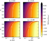 |
Fig. 10 Ratio of short-range forces to Kozai–Lidov precession rate as a function of the initial semi-major axis and eccentricity of TOI-858 B b’s orbit for four different values of TOI-858 A’s orbital eccentricity. The white dashed lines show |

5 Discussion and conclusions
The planet TOI-858 B b may represent another case of a “perpendicular planet”, adding statistical weight to the trend identified by Albrecht et al. (2021). Even though we lack an unambiguous measurement of the stellar inclination in order to disentangle the sky-projected and the true spin-orbit angle, we can still assert the polar nature of the orbit, as λ is very well constrained (Sect. 4.1.4). Moreover, the sky-projected and the 3D spin-orbit angle tend to be close when the former is near 90° (Fabrycky & Winn 2009). In any case, because of TOI-858 A’s wide separation, a Kozai–Lidov mechanism is unlikely to be the origin of TOI-858 B b’s highly misaligned orbit. With the current orbital parameters, such an effect raised by the binary companion would be cancelled out by short-range forces between TOI-858 B and its orbiting planet. Other explanations for a polar orbit include stellar flybys (e.g., Rodet et al. 2021), secular resonance crossings (Petrovich et al. 2020), and magnetic warping (e.g., Romanova et al. 2021). The flyby scenario would be compatible with the orbit of the companion star TOI-858 A; however, more precise astrometry would be needed to determine the exact nature of its orbit. Alternatively, the present wide binary stars TOI-858 A and B could have been closer together in the past, allowing for the high-eccentricity tidal migration to take place. This could explain the origin of the discovered hot Jupiter TOI-858 B b as well as the polar spin-angle misalignment that we measured in this study (Vick et al. 2023). Theoretical work is needed to assess the feasibility of such a scenario. Future observations will reveal if hot and misaligned giant planets correlate with the presence of a distant stellar companion.
In this publication, we have reported the discovery of a Jovian planet transiting TOI-858 B on a polar orbit. The combined analysis of photometric, high-resolution spectroscopic, astrometric, and imaging observations has led to the following main results:
From the joint transit photometry and RV analysis of planet TOI-858 B b, we find that it is on a 3.2797178 ± 0.0000014 day orbit around its 1.08 M⊙ G0 host star. The planet has a mass of
 MJ and a radius of 1.255 ± 0.039 RJ;
The Rossiter-McLaughlin Revolutions analysis leads to the conclusion that the planet is on a polar orbit with a sky-projected obliquity of
 ;
;Assuming that the photometric periodicity is from the host star, we find that the stellar spin axis and normal to the orbital plane are nearly perpendicular, and due to the fact that λ is so well constrained, this result does not strongly depend on the assumed rotation period;
From our combined RV-astrometry analysis, we conclude that TOI-858 B and TOI-858 A are indeed the two components of a binary system, and if the Gaia EDR3 solutions are accurate, they recently became unbound;
From our dynamical study, we conclude that Kozai-Lidov can be excluded as a possible explanation for the polar orbit of TOI-858 Bb. However, a stellar flyby would be compatible with the current astrometry of the companion star TOI-858 A.
Acknowledgements
We would like to thank the anonymous referee for the very constructive comments which significantly improved the scientific quality of the article. J.H. is supported by the Swiss National Science Foundation (SNSF) through the Ambizione grant #PZ00P2_180098. L.D.N. thanks the SNSF for support under Early Postdoc.Mobility grant #P2GEP2_200044. V.B. is supported by the National Centre for Competence in Research “PlanetS” from the SNSF. V.B. and M.A. are funded by the ERC under the European Union’s Horizon 2020 research and innovation programme (project SPICE DUNE, grant agreement no. 947634). A.B.D. was supported by the National Science Foundation Graduate Research Fellowship Program under Grant Number DGE-1122492. J.V. acknowledges support from the Swiss National Science Foundation (SNSF) under the Ambizione grant #PZ00P2_208945. Funding for the TESS mission is provided by NASA’s Science Mission Directorate. We acknowledge the use of public TESS data from pipelines at the TESS Science Office and at the TESS Science Processing Operations Center. This research has made use of the Exoplanet Follow-up Observation Program website, which is operated by the California Institute of Technology, under contract with the National Aeronautics and Space Administration under the Exoplanet Exploration Program. This work has made use of data from the European Space Agency (ESA) mission Gaia (https://www.cosmos.esa.int/gaia), processed by the Gaia Data Processing and Analysis Consortium (DPAC, https://www.cosmos.esa.int/web/gaia/dpac/consortium). Funding for the DPAC has been provided by national institutions, in particular the institutions participating in the Gaia Multilateral Agreement. This research has made use of the Washington Double Star Catalog maintained at the US Naval Observatory, of the SIMBAD database, operated at CDS, Strasbourg, France, and of NASA’s Astrophysics Data System Bibliographic Services. This work made use of Astropy a community-developed core Python package and an ecosystem of tools and resources for astronomy (Astropy Collaboration 2013, 2018, 2022). It also made us of the python packages pandas (pandas development team 2020; McKinney 2010), scipy (Virtanen et al. 2020), matplotlib (Hunter 2007), and numpy (Harris et al. 2020).
Appendix A Radial velocity measurements of TOI-858 Band TOI-858 A
CORALIE radial velocity follow-up observations of TOI-858 B.
CHIRON radial velocity follow-up observations of TOI-858 B.
CORALIE radial velocity follow-up observations of TOI-858 A.
Appendix B Correlation diagrams for the global RMR analysis
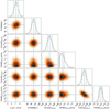 |
Fig. B.1 Correlation diagrams for the PDFs of the RMR model parameters. The CORALIE contrast and FWHM have been derived from the corresponding jump parameters to allow comparison with the observed line. The green and blue lines show the 1 and 2a simultaneous 2D confidence regions that contain, respectively, 39.3% and 86.5% of the accepted steps. The 1D histograms correspond to the distributions projected on the space of each line parameter, with the green dashed lines limiting the 68.3% HDIs. The blue lines and squares show median values. |
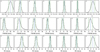 |
Fig. B.2 Posterior distribution functions of the contrast (upper panels), FWHM (middle panels), and RV centroids (lower panels) of the Gaussian line model fitted to individual CCFintr in Visit 1. The deep blue lines indicate the PDF median values, and the green dashed lines show the lσ highest density intervals. In-transit exposure indexes are shown in each subplot. |
References
- Albrecht, S. H., Marcussen, M. L., Winn, J. N., Dawson, R. I., & Knudstrup, E. 2021, ApJ, 916, L1 [NASA ADS] [CrossRef] [Google Scholar]
- Albrecht, S. H., Dawson, R. I., & Winn, J. N. 2022, PASP, 134, 082001 [NASA ADS] [CrossRef] [Google Scholar]
- Anderson, K. R., Storch, N. I., & Lai, D. 2016, MNRAS, 456, 3671 [NASA ADS] [CrossRef] [Google Scholar]
- Astropy Collaboration (Robitaille, T. P., et al.) 2013, A&A, 558, A33 [NASA ADS] [CrossRef] [EDP Sciences] [Google Scholar]
- Astropy Collaboration (Price-Whelan, A. M., et al.) 2018, AJ, 156, 123 [Google Scholar]
- Astropy Collaboration (Price-Whelan, A. M., et al.) 2022, ApJ, 935, 167 [NASA ADS] [CrossRef] [Google Scholar]
- Attia, M., Bourrier, V., Eggenberger, P., et al. 2021, A&A, 647, A40 [NASA ADS] [CrossRef] [EDP Sciences] [Google Scholar]
- Bakos, G. Torres, G., Pál, A., et al. 2010, ApJ, 710, 1724 [NASA ADS] [CrossRef] [Google Scholar]
- Baranne, A., Queloz, D., Mayor, M., et al. 1996, A&AS, 119, 373 [NASA ADS] [CrossRef] [EDP Sciences] [Google Scholar]
- Barnes, S. A. 2007, ApJ, 669, 1167 [Google Scholar]
- Batygin, K. 2012, Nature, 491, 418 [NASA ADS] [CrossRef] [Google Scholar]
- Bonfils, X., Delfosse, X., Udry, S., et al. 2013, A&A, 549, 109 [Google Scholar]
- Bouchy, F., Pepe, F., & Queloz, D. 2001, A&A, 374, 733 [NASA ADS] [CrossRef] [EDP Sciences] [Google Scholar]
- Bouchy, F., Doyon, R., Artigau, É., et al. 2017, The Messenger, 169, 21 [NASA ADS] [Google Scholar]
- Bouma, L. G., Curtis, J. L., Hartman, J. D., Winn, J. N., & Bakos, G. Á. 2021, AJ, 162, 197 [NASA ADS] [CrossRef] [Google Scholar]
- Bourrier, V., & Hébrard, G. 2014, A&A, 569, A65 [NASA ADS] [CrossRef] [EDP Sciences] [Google Scholar]
- Bourrier, V., Cegla, H. M., Lovis, C., & Wyttenbach, A. 2017, A&A, 599, A33 [NASA ADS] [CrossRef] [EDP Sciences] [Google Scholar]
- Bourrier, V., Lovis, C., Beust, H., et al. 2018, Nature, 553, 477 [NASA ADS] [CrossRef] [Google Scholar]
- Bourrier, V., Lovis, C., Cretignier, M., et al. 2021, A&A, 654, A152 [NASA ADS] [CrossRef] [EDP Sciences] [Google Scholar]
- Bowler, B. P. 2016, PASP, 128, 102001 [Google Scholar]
- Buchhave, L. A., Latham, D. W., Johansen, A., et al. 2012, Nature, 486, 375 [NASA ADS] [Google Scholar]
- Cegla, H. M., Lovis, C., Bourrier, V., et al. 2016, A&A, 588, A127 [NASA ADS] [CrossRef] [EDP Sciences] [Google Scholar]
- Chatterjee, S., Ford, E. B., Matsumura, S., & Rasio, F. A. 2008, ApJ, 686, 580 [NASA ADS] [CrossRef] [Google Scholar]
- Choi, J., Dotter, A., Conroy, C., et al. 2016, ApJ, 823, 102 [Google Scholar]
- Claret, A. 2017, A&A, 600, A30 [NASA ADS] [CrossRef] [EDP Sciences] [Google Scholar]
- Claret, A., & Bloemen, S. 2011, A&A, 529, A75 [NASA ADS] [CrossRef] [EDP Sciences] [Google Scholar]
- Collier Cameron, A., Pollacco, D., Street, R. A., et al. 2006, MNRAS, 373, 799 [Google Scholar]
- Collier Cameron, A., Bruce, V. A., Miller, G. R. M., Triaud, A. H. M. J., & Queloz, D. 2010, MNRAS, 403, 151 [NASA ADS] [CrossRef] [Google Scholar]
- Collins, K. A., Kielkopf, J. F., Stassun, K. G., & Hessman, F. V. 2017, AJ, 153, 77 [Google Scholar]
- Collins, K., Quinn, S. N., Latham, D. W., et al. 2018, in Am. Astron. Soc. Meeting Abstracts, 231, 439.08 [NASA ADS] [Google Scholar]
- Dawson, R. I., & Johnson, J. A. 2018, ARA&A, 56, 175 [Google Scholar]
- Dotter, A. 2016, ApJS, 222, 8 [Google Scholar]
- Eastman, J., Gaudi, B. S., & Agol, E. 2013, PASP, 125, 83 [Google Scholar]
- Eastman, J. D., Rodriguez, J. E., Agol, E., et al. 2019, ArXiv e-prints [arXiv: 1907.09480] [Google Scholar]
- Eastman, J. D., Diamond-Lowe, H., & Tayar, J. 2023, AJ, 166, 132 [NASA ADS] [CrossRef] [Google Scholar]
- Eggleton, P. P., & Kiseleva-Eggleton, L. 2001, ApJ, 562, 1012 [NASA ADS] [CrossRef] [Google Scholar]
- El-Badry, K., Rix, H.-W., & Heintz, T. M. 2021, MNRAS, 506, 2269 [NASA ADS] [CrossRef] [Google Scholar]
- Fabrycky, D., & Tremaine, S. 2007, ApJ, 669, 1298 [NASA ADS] [CrossRef] [Google Scholar]
- Fabrycky, D. C., & Winn, J. N. 2009, ApJ, 696, 1230 [NASA ADS] [CrossRef] [Google Scholar]
- Fischer, D. A., & Valenti, J. 2005, ApJ, 622, 1102 [NASA ADS] [CrossRef] [Google Scholar]
- Fontanive, C., & Bardalez Gagliuffi, D. 2021, Front. Astron. Space Sci., 8, 16 [NASA ADS] [CrossRef] [Google Scholar]
- Foreman-Mackey, D., Hogg, D. W., Lang, D., & Goodman, J. 2013, PASP, 125, 306 [Google Scholar]
- Foucart, F., & Lai, D. 2011, MNRAS, 412, 2799 [NASA ADS] [CrossRef] [Google Scholar]
- Gaia Collaboration (Prusti, T., et al.) 2016, A&A, 595, A1 [NASA ADS] [CrossRef] [EDP Sciences] [Google Scholar]
- Gaia Collaboration (Brown, A. G. A., et al.) 2021, A&A, 649, A1 [NASA ADS] [CrossRef] [EDP Sciences] [Google Scholar]
- Hamers, A. S., & Tremaine, S. 2017, AJ, 154, 272 [NASA ADS] [CrossRef] [Google Scholar]
- Harris, C. R., Millman, K. J., van der Walt, S. J., et al. 2020, Nature, 585, 357 [NASA ADS] [CrossRef] [Google Scholar]
- Hirsch, L. A., Rosenthal, L., Fulton, B. J., et al. 2021, AJ, 161, 134 [NASA ADS] [CrossRef] [Google Scholar]
- Høg, E., Fabricius, C., Makarov, V. V., et al. 2000, A&A, 355, A27 [NASA ADS] [Google Scholar]
- Huang, C. X., Vanderburg, A., Pál, A., et al. 2020a, RNAAS, 4, 204 [Google Scholar]
- Huang, C. X., Vanderburg, A., Pál, A., et al. 2020b, RNAAS, 4, 206 [NASA ADS] [Google Scholar]
- Hunter, J. D. 2007, Comput. Sci. Eng., 9, 90 [NASA ADS] [CrossRef] [Google Scholar]
- Jenkins, J. M., Chandrasekaran, H., McCauliff, S. D., et al. 2010, Proc. SPIE, 7740, 77400D [NASA ADS] [CrossRef] [Google Scholar]
- Jenkins, J. M., Twicken, J. D., McCauliff, S., et al. 2016, Proc. SPIE, 9913, 99133E [Google Scholar]
- Jensen, E. 2013, Astrophysics Source Code Library [record ascl:1306.007] [Google Scholar]
- Jones, M. I., Brahm, R., Espinoza, N., et al. 2019, A&A, 625, A16 [NASA ADS] [CrossRef] [EDP Sciences] [Google Scholar]
- Keivan, G., Oelkers, R. J., Paegert, M., et al. 2019, AJ, 158, 138 [NASA ADS] [CrossRef] [Google Scholar]
- Kipping, D. M., Dunn, W. R., Jasinski, J. M., & Manthri, V. P. 2012, MNRAS, 421, 1166 [NASA ADS] [CrossRef] [Google Scholar]
- Kouwenhoven, M. B. N., Goodwin, S. P., Parker, R. J., et al. 2010, MNRAS, 404, 1835 [NASA ADS] [Google Scholar]
- Kozai, Y. 1962, AJ, 67, 591 [Google Scholar]
- Kraus, A. L., Ireland, M. J., Huber, D., Mann, A. W., & Dupuy, T. J. 2016, AJ, 152, 8 [NASA ADS] [CrossRef] [Google Scholar]
- Kreidberg, L. 2015, PASP, 127, 1161 [Google Scholar]
- Law, N. M., Morton, T., Baranec, C., et al. 2014, ApJ, 791, 35 [NASA ADS] [CrossRef] [Google Scholar]
- Lidov, M. L. 1962, Planet. Space Sci., 9, 719 [Google Scholar]
- Lindegren, L. 2018, GAIA-C3-TN-LU-LL-124, Technical Note [Google Scholar]
- Liu, B., Muñoz, D. J., & Lai, D. 2015, MNRAS, 447, 747 [NASA ADS] [CrossRef] [Google Scholar]
- Mandel, K., & Agol, E. 2002, ApJ, 580, L171 [Google Scholar]
- Mason, B. D., Wycoff, G. L., Hartkopf, W. I., Douglass, G. G., & Worley, C. E. 2001, AJ, 122, 3466 [Google Scholar]
- Masuda, K., & Winn, J. N. 2020, AJ, 159, 81 [NASA ADS] [CrossRef] [Google Scholar]
- Maxted, P. F. L., Anderson, D. R., Collier Cameron, A., et al. 2011, PASP, 123, 547 [NASA ADS] [CrossRef] [Google Scholar]
- McKinney, W. 2010, in Proceedings of the 9th Python in Science Conference, eds. Stéfan van der Walt, & Jarrod Millman, 56 [CrossRef] [Google Scholar]
- McLaughlin, D. B. 1924, ApJ, 60, 22 [Google Scholar]
- Moeckel, N., & Bate, M. R. 2010, MNRAS, 404, 721 [NASA ADS] [CrossRef] [Google Scholar]
- Morris, B. M., Hawley, S. L., Hebb, L., et al. 2017, ApJ, 848, 58 [NASA ADS] [CrossRef] [Google Scholar]
- Moutou, C., Vigan, A., Mesa, D., et al. 2017, A&A, 602, A87 [NASA ADS] [CrossRef] [EDP Sciences] [Google Scholar]
- Mulders, G. D., Pascucci, I., & Apai, D. 2015, ApJ, 798, 112 [Google Scholar]
- Naoz, S. 2016, ARA&A, 54, 441 [Google Scholar]
- Ngo, H., Knutson, H. A., Hinkley, S., et al. 2016, ApJ, 827, 8 [Google Scholar]
- Offner, S. S. R., Moe, M., Kratter, K. M., et al. 2023, ASP Conf. Ser., 534, 275 [NASA ADS] [Google Scholar]
- pandas development team 2020, https://doi.org/10.5281/zenodo.8301632 [Google Scholar]
- Pearce, L. A., Kraus, A. L., Dupuy, T. J., Mann, A. W., & Huber, D. 2021, ApJ, 909, 216 [NASA ADS] [CrossRef] [Google Scholar]
- Pecaut, M. J., & Mamajek, E. E. 2013, ApJS, 208, 9 [Google Scholar]
- Pepe, F., Mayor, M., Galland, F., et al. 2002a, A&A, 388, 632 [NASA ADS] [CrossRef] [EDP Sciences] [Google Scholar]
- Pepe, F., Mayor, M., Rupprecht, G., et al. 2002b, The Messenger, 110, 9 [NASA ADS] [Google Scholar]
- Petrovich, C., Muñoz, D. J., Kratter, K. M., & Malhotra, R. 2020, ApJ, 902, L5 [NASA ADS] [CrossRef] [Google Scholar]
- Pollacco, D. L., Skillen, I., Collier Cameron, A., et al. 2006, PASP, 118, 1407 [NASA ADS] [CrossRef] [Google Scholar]
- Queloz, D., Casse, M., & Mayor, M. 1999, ASP Conf. Ser., 185, 13 [NASA ADS] [Google Scholar]
- Queloz, D., Henry, G. W., Sivan, J. P., et al. 2001a, A&A, 379, 279 [NASA ADS] [CrossRef] [EDP Sciences] [Google Scholar]
- Queloz, D., Mayor, M., Udry, S., et al. 2001b, The Messenger, 105, 1 [NASA ADS] [Google Scholar]
- Queloz, D., Anderson, D. R., Collier Cameron, A., et al. 2010, A&A, 517, A1 [Google Scholar]
- Raimbault, M. 2020, PhD thesis, University of Geneva, Switzerland [Google Scholar]
- Ricker, G. R., Winn, J. N., Vanderspek, R., et al. 2015, J. Astron. Telesc. Instrum. Syst., 1, 014003 [Google Scholar]
- Rodet, L., Su, Y., & Lai, D. 2021, ApJ, 913, 104 [NASA ADS] [CrossRef] [Google Scholar]
- Romanova, M. M., Koldoba, A. V., Ustyugova, G. V., et al. 2021, MNRAS, 506, 372 [NASA ADS] [CrossRef] [Google Scholar]
- Rossiter, R. A. 1924, ApJ, 60, 15 [Google Scholar]
- Santos, N. C., Mayor, M., Naef, D., et al. 2002, A&A, 392, 215 [NASA ADS] [CrossRef] [EDP Sciences] [Google Scholar]
- Santos, N. C., Israelian, G., & Mayor, M. 2004, A&A, 415, 1153 [NASA ADS] [CrossRef] [EDP Sciences] [Google Scholar]
- Schlafly, E. F., & Finkbeiner, D. P. 2011, ApJ, 737, 103 [Google Scholar]
- Schlegel, D. J., Finkbeiner, D. P., & Davis, M. 1998, ApJ, 500, 525 [Google Scholar]
- Seager, S., & Mallén-Ornelas, G. 2003, ApJ, 585, 1038 [Google Scholar]
- Skrutskie, M. F. et al. 2006, AJ, 131, 1163 [NASA ADS] [CrossRef] [Google Scholar]
- Smith, J. C., Stumpe, M. C., Van Cleve, J. E., et al. 2012, PASP, 124, 1000 [Google Scholar]
- Sousa, S. G., Santos, N. C., Mayor, M., et al. 2008, A&A, 487, 373 [NASA ADS] [CrossRef] [EDP Sciences] [Google Scholar]
- Stumpe, M. C., Smith, J. C., Van Cleve, J. E., et al. 2012, PASP, 124, 985 [Google Scholar]
- Stumpe, M. C., Smith, J. C., Catanzarite, J. H., et al. 2014, PASP, 126, 100 [Google Scholar]
- Tejada Arevalo, R. A., Winn, J. N., & Anderson, K. R. 2021, ApJ, 919, 138 [NASA ADS] [CrossRef] [Google Scholar]
- Teyssandier, J., Terquem, C., & Papaloizou, J. C. B. 2013, MNRAS, 428, 658 [NASA ADS] [CrossRef] [Google Scholar]
- Tokovinin, A. 2018, PASP, 130, 035002 [Google Scholar]
- Tokovinin, A., Fischer, D. A., Bonati, M., et al. 2013, PASP, 125, 1336 [NASA ADS] [CrossRef] [Google Scholar]
- Triaud, A. H. M. J. 2018, The Rossiter-McLaughlin Effect in Exoplanet Research (Springer International Publishing AG), 2 [Google Scholar]
- Udry, S., & Santos, N. C. 2007, ArA&A, 45, 397 [NASA ADS] [CrossRef] [Google Scholar]
- Vick, M., Su, Y., & Lai, D. 2023, ApJ, 943, L13 [NASA ADS] [CrossRef] [Google Scholar]
- Virtanen, P., Gommers, R., Oliphant, T. E., et al. 2020, Nat. Methods, 17, 261 [Google Scholar]
- Wang, S., Wu, D.-H., Barclay, T., & Laughlin, G. P. 2017, ArXiv e-prints [arXiv: 1704.04290] [Google Scholar]
- Wehbe, B., Cabral, A., Martins, J. H. C., et al. 2020, MNRAS, 491, 3515 [CrossRef] [Google Scholar]
- Wei, L., Naoz, S., Faridani, T., & Farr, W. M. 2021, ApJ, 923, 118 [NASA ADS] [CrossRef] [Google Scholar]
- Winn, J. N., & Fabrycky, D. C. 2015, ARA&A, 53, 409 [Google Scholar]
- Wright, E. L., Eisenhardt, P. R. M., Mainzer, A. K., et al. 2010, AJ, 140, 1868 [Google Scholar]
- Yee, S. W., Petigura, E. A., & von Braun, K. 2017, ApJ, 836, 77 [Google Scholar]
- Zanazzi, J. J., & Lai, D. 2018, MNRAS, 478, 835 [NASA ADS] [CrossRef] [Google Scholar]
- Zhu, W., & Dong, S. 2021, ARA&A, 59, 291 [NASA ADS] [CrossRef] [Google Scholar]
- Ziegler, C., Tokovinin, A., Briceño, C., et al. 2020, AJ, 159, 19 [Google Scholar]
- Ziegler, C., Tokovinin, A., Latiolais, M., et al. 2021, AJ, 162, 192 [NASA ADS] [CrossRef] [Google Scholar]
All Tables
Summary of the discovery TESS photometry, archival WASP-South photometry, and ground-based follow-up photometry of TOI-858 B.
All Figures
|
Fig. 1 Photometric transit observations of TOI-858 B b in 20 min bins. The vertical dashed lines represent meridian flips. The bottom panel shows all light curves phase folded and overplotted. |
| In the text | |
|
Fig. 2 SOAR speckle imaging in Cousins I-band excluding nearby stars down to A Imag ~5 within 3″ of TOI-858 B. The inset is the speckle ACF centred on the target star. |
| In the text | |
|
Fig. 3 Periodograms showing the stellar rotational modulation in the WASP-South and TESS data, spanning 11 years in total. All data sets indicate a rotation period of 6.4−6.2 days. The vertical blue lines in all four panels indicate Prot = 6.42 days, determined using the WASP-South data (200 mm and 85 mm). |
| In the text | |
|
Fig. 4 Phase folded CORALIE and CHIRON RV measurements for TOI-858 B. |
| In the text | |
|
Fig. 5 CORALIE RV measurements of TOI-858 A. Top panel: RV time series showing no clear signs of a giant planet in a short period orbit. Lower panel: Lomb–Scargle periodogram for the RVs with no significant signals detected. The false alarm probability (FAP) levels of 1% and 10% are indicated as horizontal lines. |
| In the text | |
|
Fig. 6 Maps of the CCFintr during the transit of TOI-858 B b in Visit 1 (upper panel) and Visit 2 (lower panel). Transit contacts are shown as green horizontal dashed lines. Values are coloured as a function of their normalised flux and plotted as a function of RV in the stellar rest frame (in abscissa) and orbital phase (in ordinate). The stellar lines from the planet-occulted regions are clearly visible in both visits. The green solid lines show the best-fit model for the stellar surface RVs derived from a joint RMR fit to both data sets. The green vertical dashed lines show the spectroscopic, sky-projected stellar rotational velocity. |
| In the text | |
|
Fig. 7 Properties of the stellar surface regions occulted by TOI-858 B b. in blue for Visit 1 and red for Visit 2. The dashed vertical lines are the transit contacts. The horizontal bars indicate the duration of each exposure. The vertical bars indicate the 1σ HDI intervals. The solid curves are the best models to each property, derived from a joint RMR fitted to both visits (excluding the first exposure in Visit 2). The RV model is common to both visits. The model contrast and FWHM are specific to each visit and are shown here after convolution of the model line by the CORALIE line spread function (LSF). |
| In the text | |
|
Fig. 8 Maps of the out-oſ-transit residuals and of the in-transit residuals between CCFintr and their best-fit model in Visit 1 (top panel) and Visit 2 (bottom panel). Transit contacts are shown as green dashed lines. The green vertical dashed lines show the spectroscopic, sky-projected stellar rotational velocity. |
| In the text | |
|
Fig. 9 Projection of TOI-858 B in the plane of sky for the best-fit orbital architecture. The black arrow shows the sky-projected stellar spin. The stellar disc is coloured as a function of its surface RV field. The normal to the orbital plane of TOI-858 B b is shown as a green arrow. The thick green solid curve represents the best-fit orbital trajectory. The thin lines surrounding it show orbits obtained for orbital inclination, semi-major axis, and sky-projected obliquity values drawn randomly within 1σ from their probability distributions. The star, planet (black disc), and orbits are to scale. |
| In the text | |
|
Fig. 10 Ratio of short-range forces to Kozai–Lidov precession rate as a function of the initial semi-major axis and eccentricity of TOI-858 B b’s orbit for four different values of TOI-858 A’s orbital eccentricity. The white dashed lines show |
| In the text | |
|
Fig. B.1 Correlation diagrams for the PDFs of the RMR model parameters. The CORALIE contrast and FWHM have been derived from the corresponding jump parameters to allow comparison with the observed line. The green and blue lines show the 1 and 2a simultaneous 2D confidence regions that contain, respectively, 39.3% and 86.5% of the accepted steps. The 1D histograms correspond to the distributions projected on the space of each line parameter, with the green dashed lines limiting the 68.3% HDIs. The blue lines and squares show median values. |
| In the text | |
|
Fig. B.2 Posterior distribution functions of the contrast (upper panels), FWHM (middle panels), and RV centroids (lower panels) of the Gaussian line model fitted to individual CCFintr in Visit 1. The deep blue lines indicate the PDF median values, and the green dashed lines show the lσ highest density intervals. In-transit exposure indexes are shown in each subplot. |
| In the text | |
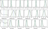 |
Fig. B.3 Same as Fig. B.2 but for Visit 2. |
| In the text | |
Current usage metrics show cumulative count of Article Views (full-text article views including HTML views, PDF and ePub downloads, according to the available data) and Abstracts Views on Vision4Press platform.
Data correspond to usage on the plateform after 2015. The current usage metrics is available 48-96 hours after online publication and is updated daily on week days.
Initial download of the metrics may take a while.