| Issue |
A&A
Volume 686, June 2024
|
|
|---|---|---|
| Article Number | A147 | |
| Number of page(s) | 19 | |
| Section | Planets and planetary systems | |
| DOI | https://doi.org/10.1051/0004-6361/202349084 | |
| Published online | 10 June 2024 | |
Stellar obliquity measurements of six gas giants
Orbital misalignment of WASP-101b and WASP-131b
1
European Southern Observatory,
Karl-Schwarzschild-str. 2,
85748
Garching,
Germany
e-mail: This email address is being protected from spambots. You need JavaScript enabled to view it.
2
Astronomical Institute of the Czech Academy of Sciences,
Fričova 298,
25165
Ondřejov,
Czech Republic
3
Faculty of Physics and Astronomy, Friedrich-Schiller-Universität,
Fürstengraben 1,
07743
Jena,
Germany
4
Dipartimento di Fisica, La Sapienza Università di Roma,
Piazzale Aldo Moro 5,
Roma
00185,
Italy
5
European Southern Observatory,
Casilla 13,
Vitacura,
Santiago, Chile
6
European Space Agency (ESA), ESA Office, Space Telescope Science Institute (STScI),
Baltimore,
MD
21218,
USA
7
Department of Theoretical Physics and Astrophysics, Masaryk University,
Kotlářská 2,
61137
Brno,
Czech Republic
8
Thueringer Landessternwarte Tautenburg,
Sternwarte 5,
07778
Tautenburg,
Germany
Received:
22
December
2023
Accepted:
19
March
2024
Abstract
One can infer the orbital alignment of exoplanets with respect to the spin of their host stars using the Rossiter-McLaughlin effect, thereby giving us the chance to test planet formation and migration theories and improve our understanding of the currently observed population. We analyzed archival HARPS and HARPS-N spectroscopic transit time series of six gas giant exoplanets on short orbits, namely WASP-77 Ab, WASP-101b, WASP-103b, WASP-105b, WASP-120b, and WASP-131b. We find a moderately misaligned orbit for WASP-101b (λ = 34° ± 3) and a highly misaligned orbit for WASP-131b (λ = 161° ± 5), while the four remaining exoplanets appear to be aligned: WASP-77 Ab (λ = −8°−18+19), WASP-103b (λ = −2°−36+35), WASP-105b (λ = −14°−24+28), and WASP-120b (λ = −2° ± 4). For WASP-77 Ab, we are able to infer its true orbital obliquity (Ψ = 48°−21+22). We additionally performed transmission spectroscopy of the targets in search of strong atomic absorbers in the exoatmospheres, but were unable to detect any features, most likely due to the presence of high-altitude clouds or Rayleigh scattering muting the strength of the features. Finally, we comment on future perspectives on studying these planets with upcoming space missions to investigate their evolution and migration histories.
Key words: techniques: radial velocities / planets and satellites: atmospheres / planets and satellites: gaseous planets / planet-star interactions
© The Authors 2024
 Open Access article, published by EDP Sciences, under the terms of the Creative Commons Attribution License (https://creativecommons.org/licenses/by/4.0), which permits unrestricted use, distribution, and reproduction in any medium, provided the original work is properly cited.
This article is published in open access under the Subscribe to Open model. This email address is being protected from spambots. You need JavaScript enabled to view it. to support open access publication.
1 Introduction
The formation and evolution of exoplanets and how this is linked to the properties of their host stars and the environments in which they formed are long-standing questions. One possible clue may come from measuring the relative angle of the rotation axis of the star with that of the planetary orbital angular momentum. The planets of the Solar System, for example, are almost co-planar, as these angles – called stellar obliquities – are all very small, leading to the idea of planet formation within a disk. The sky-projected stellar obliquity can be inferred through the observations of the Rossiter-McLaughlin (R-M) effect, which is a spectroscopic anomaly that occurs when the disk of a companion passes in front of the spinning star. As usual in astronomy, this effect is misnamed, as it was first described by Holt (1893), and then actually detected in the binary system β Lyrae by Rossiter (1924). The same year, and using the methodology of Rossiter, McLaughlin (1924) applied it to a study of Algol, while the first application of the R-M effect to exoplanets was carried out by Queloz et al. (2000) on HD 209458. For a more detailed review of this history, the reader is encouraged to refer to Albrecht et al. (2011, 2022). At first, only Jupiter-mass planets were characterized, but later development of instrumentation allowed for the characterization of Neptunian (Bourrier et al. 2018), sub-Neptunian (Dalal et al. 2019), and even terrestrial planets (Hirano et al. 2020; Zhao et al. 2022). Such studies have revealed a complex architecture of exoplanetary systems with planetary orbits varying from well aligned, to slightly misaligned, to planets on polar and even retrograde orbits.
The R-M effect is thus a valuable tool as it can provide an insight into planetary formation and evolution (Triaud 2018). It can be used to test theories of planetary migration, for example to understand if the planet formed in situ or if it migrated to its current location. Polar and retrograde orbits are indicative of a violent history within the system, as such orbits seem to oppose the standard formation processes for the planetary systems where both the star and the planets form from the same rotating disk. Several mechanisms have been proposed to explain these extreme orbits, such as long-term interactions with a binary companion (Batygin 2012), close flybys of other stars (Bate et al. 2010), the shift of the stellar rotation axis relative to the disk due to the effects of the stellar magnetic field (Lai et al. 2011), gravitational scattering among the planets (Chatterjee et al. 2008), or long-term perturbations due to a companion caused by the Kozai-Lidov mechanism (Fabrycky & Tremaine 2007). Breslau & Pfalzner (2019) showed that retrograde orbits can also be the outcome of prograde flybys.
Despite the large number (over 150) of R-M effect measurements, there are no definitive trends in the planetary population when plotting the projected obliquity versus other parameters.
However, some trends have been tentatively proposed. Albrecht et al. (2012) and Dawson (2014) identified two populations of hot Jupiters, based on the effective temperature of the host star, with the division being located at the Kraft break – an abrupt decrease in the stars’ average rotation rates at about 6200 K (Kraft 1967). Rice et al. (2022) find evidence that warm Jupiters in single-star systems form more quiescently compared to their hot analogues. Hamer & Schlaufman (2022) find that hot Jupiter host stars with larger-than-median obliquities are older than hot Jupiter host stars with smaller-than-median obliquities. In this study, we present the projected obliquity measurements of six gas giants on short orbital periods around F-G-K dwarfs with previously unpublished HARPS and HARPS-N archival data.
Observing logs of all six planets.
2 Datasets and their analyses
We have used datasets for five exoplanets from ESO’s HARPS instrument mounted at the 3.6-m telescope at La Silla, Chile. Furthermore, the data for one planet (WASP-103) were obtained with the HARPS-N instrument mounted at the 3.5-m TNG telescope at La Palma, Canary Islands. The HARPS data were downloaded from the ESO science archive1 (program IDs 0102.C-0618, 096.C-0331, 094.C-0090, 0102.C-0319, and 095.C-0105), while the HARPS-N data (program ID A33TAC17) were obtained from the TNG archive2. Table 1 displays the properties of the datasets that were used. The downloaded data are fully reduced products as processed with the HARPS Data Reduction Software (DRS version 3.8). Each spectrum is provided as a merged 1D spectrum resampled onto a 0.001 nm uniform wavelength grid. The wavelength coverage of the spectra spans from 380 to 690 nm, with a resolving power of R ≈ 115 000 corresponding to 2.7 km s−1 per resolution element. The spectra are already corrected to the Solar system barycentric frame of reference. We further summarize the properties of the studied systems in Table 2.
2.1 Rossiter–McLaughlin effect
The radial velocities measured during the transit show the anomaly produced by the R-M effect. We retrieved the radial velocity measurements that were obtained from the HARPS and HARPS-N DRS pipeline together with their uncertainties. To measure the projected stellar obliquity of the system (λ), we fit the radial velocity data with a subroutine from the RADVEL package (Fulton et al. 2018) that assumes a Keplerian orbit and the R-M effect formulation of AROMEPY3 (Sedaghati et al. 2023), which is a Python translation of the AROME code (Boué et al. 2013). We used the R-M effect function defined for radial velocities determined through the cross-correlation technique in our code. We fixed the radial velocity semi-amplitude, K, to the literature value and allowed the systemic velocity, γ, to be a free parameter. In the R-M effect model, we fixed the following parameters to those reported in the literature: the orbital period, P, the planet-to-star radius ratio, Rp/Rs, and the eccentricity, e. The parameter σ, which is the width of the cross-correlation function (CCF) (full width at half maximum of a Gaussian fit to the CCF), was measured on the data and fixed. Furthermore, we used the EXOCTK4 tool to compute the quadratic limb-darkening coefficients in the wavelength range of the HARPS and HARPS-N instruments (380–690 nm). We allowed the following parameters to be free during the fitting procedure within the priors from photometry: the central transit time, TC, the projected stellar rotational velocity, υ sin i*, the sky-projected angle between the stellar rotation axis and the normal of the orbital plane, λ, the orbital inclination, i, and the scaled semi-major axis, a/Rs. To obtain the best-fitting values of the parameters we employed three independent Markov chain Monte Carlo (MCMC) simulations, each with 250 000 steps, burning the first 50 000. Using this setup, we obtained our results, which we present in Sect. 3.1 and in Figs. 1–6.
2.2 Transmission spectroscopy
We performed transmission spectroscopy of our targets, following the methodology performed by Wyttenbach et al. (2015) and Žák et al. (2019). First, to correct for telluric emission lines we used fiber B, which was aimed at the adjacent sky, and we used the Molecfit software (Smette et al. 2015; Kausch et al. 2015). Molecfit uses synthetic modeling of the Earth’s atmospheric spectrum with a line-by-line approach. We carefully selected nine telluric wavelength regions in the range of 589–651 nm. These regions contain unblended telluric lines produced by H2O and O2. The best-fit Molecfit solution was applied to the whole HARPS spectra. As the next step, we shifted all the spectra to the stellar rest frame. We performed a wavelength cut to isolate the region of interest and performed flux normalization for the spectra. Normalization was done in IRAF (Tody 1986) using the task continuum and on the regions of the spectra without strong lines. Subsequently, we averaged all out-of-transit spectra to create a stellar template. We divided each spectrum during transit by this template to obtain individual transmission spectra. Such spectra need to be corrected for the planetary motion of the planet. These corrected residuals were summed up and normalized to unity. Finally, unity was subtracted to obtain the final transmission spectrum,  :
:
 (1)
(1)
In principle, stellar activity might hinder our ability to retrieve any planetary signal (e.g., Barnes et al. 2017). To assess the impact of stellar activity on the transmission spectra, we repeated our methodology on several control lines (Mg I and Ca I). We retrieve a flat spectrum consistent with a negligible effect of the stellar activity.
Properties of the targets (star and planet).
3 Results
3.1 Projected stellar obliquity measurement
We measured the projected stellar obliquity (λ) of four targets for the first time: WASP-77 Ab, WASP-101b, WASP-105b, and WASP-120b. WASP-103b has been previously studied by Addison et al. (2016) using the UCLES spectrograph. WASP-131b had its spin-orbit alignment measured by Doyle et al. (2023) using ESPRESSO during the advanced stages of preparing this manuscript.
WASP-77 Ab is an inflated hot Jupiter orbiting a G8 host star on a short 1.4 day orbit. The host star has a fainter companion at a distance of 3 arcsec (Maxted et al. 2013). We infer an aligned orbit of WASP-77 Ab, with  .
.
WASP-101b is a highly inflated hot Jupiter orbiting a F6 host star on a 3.5 day orbit. We infer a misaligned orbit of WASP-101b, with λ = 34 ± 3 deg.
WASP-103b is an ultrahot Jupiter orbiting an F8 host star on a 0.92 day orbit. Wöllert & Brandner (2015) discovered a nearby source that Southworth & Evans (2016) characterized as a 0.72 ± 0.08 M⊙ star in the WASP-103 system. The system has been frequently observed (e.g., Maciejewski et al. 2018; Delrez et al. 2018; Patra et al. 2020) for possible period changes. Recent CHEOPS observations found a hint of an orbital period increase due to tidal decay (Barros et al. 2022). We infer an aligned orbit of WASP-103b with  . The derived projected obliquity is in agreement with the results of Addison et al. (2016) who obtained λ = 3 ± 33 deg.
WASP-105b is a warm Jupiter-sized planet. It orbits its K2 host star on a 7.8 day orbit. We infer an aligned orbit, with  .
.
WASP-120b is a massive hot Jupiter. It orbits its F5 host star on a 3.6 day, slightly eccentric orbit (e = 0.05). Bohn et al. (2020) found a possible binary companion, but furtherastromet-ric data are needed to confirm the tertiary nature of the system. We find that the orbit of WASP-120b is well aligned, with λ = −2 ± 4 deg.
WASP-131b is a highly inflated hot Saturn. It orbits its G0 host star on a 5.3 day orbit. WASP-131 has a low-mass stellar companion (Bohn et al. 2020; Southworth et al. 2020). We infer a highly misaligned orbit of WASP-131b, with λ =161 ± 5 deg. Our results based on HARPS data are in excellent agreement with the results from ESPRESSO,  (Doyle et al. 2023).
The results of our fits are shown in Figs. 1–6, while the MCMC results are shown in Figs. B1–B6 of the appendix. The derived values from the MCMC analysis are displayed in Table 3.
The values of υ sin i* that we derived in our R-M effect analysis are generally in agreement with the ones reported in the literature from spectral synthesis. A discrepancy is, however, observed for WASP-77 A. Hence, we measured the υ sin i* from our HARPS stacked spectra using iSpec (Blanco-Cuaresma et al. 2014). We obtained a value of υ sin i* = 2.6 ± 0.4 km s−1, in better agreement with the value obtained from our R-M effect analysis in Table 3.
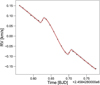 |
Fig. 1 Rossiter-Mclaughlin effect of WASP-77 Ab observed with HARPS. The observed data points (black) are shown with their error bars, which in this case are smaller than the symbol size. The systemic velocity was removed for better visibility. The red line shows the model that fits the data best, together with 1σ (dark gray) and 3σ (light gray) confidence intervals. |
MCMC analysis results.
3.2 Transmission spectroscopy
With the same datasets that were used to measure the projected stellar obliquity we also performed transmission spectroscopy to search for strong optical absorbers such as sodium (589 nm doublet) and hydrogen (Balmer alpha). The most amenable targets are WASP-101b and WASP-131b, thanks to their high transmission spectroscopy metric (TSM), which rates the suitability of the target for atmospheric characterization (Kempton et al. 2018) – see Table 4. For all the targets, we derive featureless spectra and show in Figs. 7 and 8 the sodium doublet regions forWASP-101b and WASP-131b around the sodium doublet. The results for WASP-101b are in agreement with the previous studies using the Hubble Space Telescope (HST) in the near-infrared (NIR) and optical region (Wakeford et al. 2017a; Rathcke et al. 2023) that found featureless spectra and attributed them to the presence of thick clouds. While in Fig. 7 the sodium D1 appears to have two points in the absorption, we do not claim a detection, especially as the sodium D2 line is predicted to have a more profound line profile (Gebek & Oza 2020) that we do not detect in our spectra. We have compared the observed spectrum with a clear atmosphere model and a featureless spectrum using a χ2 test and the featureless model is preferred.
WASP-103b is an accessible target for the investigation of Balmer-driven mass loss due to its proximity to the host star (García Muñoz & Schneider 2019). We derive a featureless spectrum around the H-alpha region. We provide the first transmission spectrum of WASP-131b which is expected to have a large atmospheric signal. The derived spectrum shows no absorption features and possibly hints at either, the presence of clouds, Rayleigh scattering muting the strength of the absorption features, and/or processes depleting sodium (Iro et al. 2005).
Transmission (TSM) and emission (ESM) spectroscopy metrics for our sample, as defined in Kempton et al. (2018).
4 Discussion
4.1 Misaligned planets
We compare our results to the known sample5 of exoplan-ets with measured spin-orbit alignment (Fig. 9). WASP-131b resides in the less populated region of highly-misaligned planets with host star temperature lower than 6250 K. This temperature corresponds to the Kraft break, which separates stars with deep convective envelopes and efficient magnetic dynamos from those without (Maeder 2009; Avallone et al. 2022). As noted in Albrecht et al. (2022), most of the planets that are on retrograde orbits around cooler stars are planets with Neptunian masses. WASP-131b is one of the most misaligned Saturn-mass planets known and is an especially intriguing target for migration theories as it is known that its host has a stellar companion on wide orbit (Bohn et al. 2020). The Kozai-Lidov mechanism (Fabrycky & Tremaine 2007) can put a planet on a retrograde orbit in the presence of a wide stellar companion. As the orbit has already been circularized through tidal interactions with the host star, we cannot confirm this scenario. However, future atmospheric chemistry studies may be able to provide clues about the position in the disk where the planet formed (Madhusudhan et al. 2014).
WASP-101b with its projected obliquity of 34 degrees joins a less populated region of misaligned planets (Figs. 9 and 10). A trend (Albrecht et al. 2021; Attia et al. 2023) suggests that misaligned planets do not equally cover the full range of obliquities but they rather show a preference for polar orbits (λ ~ 90 deg). However, the mechanisms responsible for this trend are still under debate (Lai 2012; Petrovich et al. 2020; Siegel et al. 2023). Furthermore, Dong & Foreman-Mackey (2023) reported that misaligned systems have nearly isotropic stellar obliquities with no strong clustering near 90 degrees. These contradictory findings warrant a further investigation of the distribution of misaligned planets. The other targets join a well-populated parameter space of aligned gas giant exoplanets.
We tried to assess whether misaligned Jupiter-mass planets around hot stars belong to a different population of exoplanets. To this end, we performed6 a two-dimensional KS test (Peacock 1983) to study the parameter space Teff−Mp and compared the misaligned population (λ ≥ 20 deg) to the whole gas giant population. The test reveal that, with a p-value of 1 × 10⁻¹¹, we can reject the null hypothesis that both groups originate from the same planetary population.
 |
Fig. 7 Transmission spectrum for WASP-101b showing a non-detection of any absorbers. The blue dashed lines indicate the position of the Na D2 and D1 lines. We show in cyan a simulated spectrum corresponding to a clear atmosphere model. In red we show a featureless spectrum. The latter model is preferred by a χ2 test. |
 |
Fig. 8 Transmission spectrum for WASP-131 b showing a non-detection of any absorbers. The blue dashed lines indicate the position of the Na D2 and D1 lines. |
4.2 Stellar rotation and true obliquity Ψ
Photometric light curves can sometimes be used to derive the stellar rotation periods (e.g., Skarka et al. 2022) due to modulations imprinted by the presence of active regions on the spinning star – a key ingredient to derive the stellar inclination i* and thus the true obliquity. We have tried to infer the stellar rotation periods using TESS (Ricker et al. 2015) and ASAS-SN g band (Kochanek et al. 2017) light curves, using a Lomb-Scargle periodogram (Lomb 1976; Scargle 1982). We were able to detect a periodic modulation of WASP-77 A with a period of 16.1 ± 0.15 days in the ASAS-SN data (FAP = 1 × 10⁻⁵, Fig. B7). This is in agreement with a literature value for rotational modulation for WASP-77 A detected by Maxted et al. (2013) who reported a value of 15.4 ± 0.4 days in the WASP light curve. For other targets, we were not able to detect any signal with high significance. Using the values above we infer i* = 41 ± 11 deg for WASP-77 A7. Combining the λ and i* measurements we are able to infer the true stellar obliquity Ψ using the spherical law of cosines, cosΨ = sin i* sin i cos|λ| + cos i* cos i. We obtain  degrees8.
4.3 Future atmospheric characterization
The high-resolution transmission spectroscopy method can probe the upper atmospheres of exoplanets by resolving the deep line cores of strong atomic features. Optical spectra of exoplan-ets are valuable tools for atmospheric retrievals using broadband infrared data. Such retrievals suffer from severe degeneracies as multiple combinations of parameters can fit the same dataset well. These degeneracies can be lifted by constraints provided with optical data (Welbanks & Madhusudhan 2019). The presence of the refractory elements is used to study the evolution of gas planets (Lothringer et al. 2021; Hands & Helled 2022). Our results from Sect. 3.2 will aid future missions in obtaining more precise abundances of these gas giants to unravel their history.
In the future, space and airborne missions (e.g., Ariel, Tinetti et al. 2018, Twinkle, Edwards et al. 2019b, and EXCITE, Nagler et al. 2022) will provide a homogeneous sample of exoplanetary atmospheric spectra. The European Space Agency’s Ariel9 mission, scheduled for launch in 2029, is specifically designed to conduct the first unbiased survey of a statistically significant sample of around 1000 transiting exoplanets across the visible and NIR spectrum. With limited prior information on the targets (mainly limited to their existence, radius, mass, and equilibrium temperature), Ariel’s observational strategy is based on four distinct tiers (Edwards et al. 2019a; Bocchieri et al. 2023). Tier 3 consists of repeated observations of a select group of benchmark planets (approximately 50–100) around bright stars to characterize their atmospheres in detail.
Knowing the spin-orbit orientation of planetary systems will complement the information obtained by these missions, especially in regard to the planetary formation and evolution questions. In the following subsections, we summarize atmospheric prospects for WASP-77Ab, WASP-101b, WASP-103b, and WASP-131b as these planets are the most amenable to future atmospheric studies, as is suggested by their TSMs and emission spectroscopy metrics (ESMs), reported in Table 4.
For WASP-77Ab, WASP-101b, and WASP-131b, we show the simulated atmospheric transmission spectra as would be obtained by Ariel. These spectra were produced by combining forward models from TauREx 3 (Al-Refaie et al. 2021) with the Ariel radiometric simulator, ArielRad (Mugnai et al. 2020), following the same methodology as presented in Mugnai et al. (2021). That is, for a given planet and atmospheric model, we used TauREx 3 to generate the high-resolution transmission spectrum. Then, we binned the raw spectrum to the Tier-3 spectral grid (R = 20, 100, and 30, in NIRSpec, AIRS-CH0, and AIRS-CH1, respectively) and added the associated noise predicted by ArielRad for each spectral bin. ArielRad is a wrapper of ExoRad (Mugnai et al. 2023) (the instrument-independent version of the radiometric simulator, available on GitHub10) and ArielRad-Payloads, the repository of configuration files for the payload maintained by the Ariel Consortium. For reproducibility, we report the code versions in Table 5. Finally, for WASP-103b, we show predicted JWST MIRI observations. The results for individual planets are presented in Appendix A.
 |
Fig. 9 Projected obliquity versus stellar effective temperature. Our targets are plotted with stars. The dashed vertical black line shows the position of the Kraft break. |
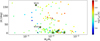 |
Fig. 10 Projected obliquity versus the ratio of the planetary to the stellar mass. Our targets are plotted with stars. |
Codes used to produce the simulated Ariel spectra.
5 Summary
We analyzed HARPS and HARPS-N archival data of six gas giant planets on short orbits around F-G-K dwarfs. We studied the R-M effect and measured the spin orbit alignment for the first time for four planets. We find that WASP-131b is on a highly misaligned orbit and joins a small number of highly misaligned planets around a host star with an effective temperature below 6250 K. WASP-101b is on a misaligned orbit, while WASP-77 Ab, WASP-103b, WASP-105b, and WASP-120b are on aligned orbits. We also derived the true (3-D) obliquity of WASP-77 Ab,  . We further performed transmission spectroscopy in order to search for strong atomic absorbers (sodium doublet and H-alpha), but obtained featureless spectra, likely due to a cloud deck at high altitudes and/or Rayleigh scattering muting the strength of the features. Finally, we discussed future perspectives on studying these planets with space missions that will be able to constrain the planets’ evolution and migration histories via atmospheric chemistry studies.
Acknowledgements
The authors would like to thank the anonymous referee for their insightful report. We would like to also thank Prune C. August for sending us model spectra. M.V. and M.S. would like to acknowledge the funding from MSMT LTT-20015. P.K. would like to acknowledge the funding from GACR 22-30516K. The funding from ANID-23-05 and HORIZON project number 101086149 enabled the mobility between Czech and Chilean colleagues (M.V. and P.K.).
Appendix A Future atmospheric characterization: Results for individual planets
Appendix A.1 WASP-77Ab
WASP-77 Ab is listed as a Tier-3 object in a recently proposed Ariel candidate sample (Edwards & Tinetti 2022), with emission spectroscopy as the preferred observing mode. Line et al. (2021) found a solar C/O ratio and subsolar metallicity in the planetary atmosphere using the Gemini telescope. The subsolar metallicity was later confirmed using the NIRSpec instrument on JWST (August et al. 2023). Line et al. (2021) suggest that WASP-77 Ab accreted its envelope interior to its parent pro-toplanetary disk’s H2O ice line from carbon-depleted gas with little subsequent planetesimal accretion or core erosion. Such mechanisms are hard to reconcile with the nonsolar abundance ratios of WASP-77 A published by Reggiani et al. (2022). They find that WASP-77 Ab likely formed outside of its parent proto-planetary disk’s H2O ice line (~ 4.5 AU) based on an enhanced C/O ratio and then migrated inwards. Khorshid et al. (2023), using the SimAb code, studied the possible pathways for the formation of this planet with different initial disk conditions. They find that the planet likely initiated its migration within the CO2 ice line (~ 15 AU) and was moved inward via disk-free migration. Our measurement of an apparent alignment of the planet’s orbit with the stellar rotation axis is in agreement with this. Finally, Changeat et al. (2022) find hints of TiO in the atmosphere. Our results find a featureless spectrum that could hint either at the presence of hazes in the optical wavelengths or at a lower abundance of refractory materials. However, future studies with higher signal-to-noise ratio (S/N) are needed to confirm the origin of the muted features.
Future characterization of WASP-77 Ab with Ariel and JWST will measure several carbon- and oxygen-bearing molecular species (such as H2O, CO, and CO2) to determine its C/O ratio with unprecedented precision and accuracy, and hence shed more light on its formation pathways. We show a simulated spectrum using one eclipse in Fig. A.1. We generated the spectrum assuming equilibrium chemistry with metallicity and C/O ratio values taken from Smith et al. (2024). A single Ariel observation will be able to unambiguously distinguish between the two currently competing models thanks to its continuous wavelength coverage from 0.5 to 7.8 µm observed simultaneously.
As is suggested by Turrini et al. (2021), additional elemental ratios (e.g., N/O, C/N, and S/N) may present a better opportunity to study the planetary formation and will provide crucial information in unambiguously determining planetary history pathways. Charnay et al. (2022) show that WASP-77 Ab would be an excellent target for studying the redistribution of the thermal energy via obtaining phase curves during various orbital phases of the planetary orbit. Phase curve studies will cover the whole orbital phase; the night side with a temperature ≈ 1000 K (Keating et al. 2019) offers the best opportunity to infer nitrogen abundances (in order to obtain the C/N and N/O ratios). Based on detailed models by Ohno & Fortney (2023), NH3 has the best chance of being detected by the JWST-MIRI instrument targeting its strong absorption band at 11 µm.
Appendix A.2 WASP-101b
Due to its high TSM, WASP-101b was initially considered as a prime candidate for transmission spectroscopy using JWST in the Early Release Science (ERS) program. However, Wakeford et al. (2017a) later measured a featureless spectrum. They observed WASP-101b in the spectral region from 1.1 to 1.7µm with HST and from the lack of spectral features inferred the possible presence of a cloud deck or of water vapor depletion. This apparently disqualified WASP-101b from the JWST ERS. A later study using HST in the optical region obtained a flat spectrum and inferred the presence of clouds (Rathcke et al. 2023). In our analysis, we have obtained results consistent with the presence of clouds yielding a featureless spectrum. Nevertheless, Kawashima et al. (2019) have shown that, even in the presence of clouds, the redder part of the JWST or Ariel spectrum can still provide useful information about the atmospheric composition. WASP-101b is categorized as a Tier-3 object in Edwards & Tinetti (2022), with transmission spectroscopy as the preferred observing mode, and we provide here a simulated transmission spectrum as would be observed by Ariel.
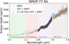 |
Fig. A.1 Simulated Ariel emission spectrum of WASP-77Ab’s atmosphere. In orange and blue we show two competing models presented in August et al. (2023). Ariel will be able to distinguish between these two models with high confidence with a single observed eclipse due to its broad wavelength coverage. |
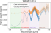 |
Fig. A.2 Simulated Ariel transmission spectra of WASP-101b’s atmosphere. In orange, we show a model with thick clouds consistent with previous HST data. In blue, we display a model with a clear atmosphere. The colors correspond to the different instruments and channels of Ariel. |
The simulated spectrum using two transits is presented in Fig. A.2. In blue, the spectrum corresponds to equilibrium chemistry with solar elemental ratios with a clear atmosphere. In orange, the simulated spectrum corresponds to equilibrium chemistry and is consistent with the muted spectral features observed with HST. This shows that, even when considering gray clouds (opaque at all wavelengths), a worst-case assumption, this does not preclude the possibility of atmospheric characterization. The spectral region between 2 and 4 µm still contains valuable information about the molecular composition – in particular, features of CO and CO2 can still be accessible for analysis, especially as CO2 is an atmospheric metallicity indicator in giant planet atmospheres (Lodders & Fegley 2002). These observations will improve our understanding of the environment where aerosols form, especially as WASP-101b might belong to a sparse class of cloudy exoplanets with an equilibrium temperature above 1 500 K. Hence, future JWST observations with the MIRI instrument might shed more light on the possible presence, origin, and composition of the aerosols (Wakeford et al. 2017b). Furthermore, MIRI will cover the strong SO2 band between 7 and 8 µm. As SO2 is expected to be present in higher layers of the atmosphere, it is less likely to be obscured, even in the presence of aerosols. SO2 has recently been suggested as a promising tracer of metallicity in giant exoplanet atmospheres (Polman et al. 2023; Tsai et al. 2023).
Appendix A.3 WASP-103b
WASP-103b is ranked in Ariel tier 3 for emission spec-troscopy (Edwards & Tinetti 2022). The atmosphere of WASP-103b has been studied by several teams in the past. Lendl et al. (2017) found the presence of strong alkali metals using the Gemini telescope. However, this result has not been confirmed by subsequent atmospheric studies (Wilson et al. 2020; Kirk et al. 2021). Our results are consistent with the null detection reported by the later studies. Changeat (2022) found hints of thermal inversion and presence of H2O, FeH, CO, and CH4 features using HST data. Recent observations with the Canada–France–Hawaii Telescope (Shi et al. 2023) confirmed the presence of thermal inversion and also detected a super-solar metallicity composition.
Due to its high temperature (2 500 K) and reportedly detected thermal inversion, WASP-103b is an excellent candidate for the detection of ionic species (Fe II, Ti II) and of metal oxides such as TiO and VO in the optical and SiO in the NIR (Gandhi & Madhusudhan 2019). Lothringer et al. (2022) report the detection of SiO for the first time in the atmosphere of an ultrahot Jupiter, WASP-178b, with a similar equilibrium temperature (~ 2450 K) to that of WASP-103b. We used TauREx3 (Al-Refaie et al. 2021) with the GGchem chemical code (Woitke et al. 2018) and the atmospheric parameters (T-p profiles, metallicity, and C/O ratios) inferred in Changeat (2022) to simulate the day-and night-side spectrum of WASP-103b with JWST MIRI phase-curve observations (noise estimated via Pandexo: Batalha et al. (2017)). We included a semi-opaque silicate cloud layer in our simulations. Our models show that SiO can easily be detected for 5x the solar Si/O ratio Fig. A.3. SiO is a refractory material and has been proposed as one of the possible origins of thermal inversions alongside other refractory materials such as TiO and VO. The detection of SiO would provide a key insight into the origin of thermal inversions, which is not fully understood (Parmen-tier et al. 2018). For ultrahot Jupiters (as they are hot enough to largely avoid the condensation of refractory species), the ratio of refractory-to-volatile elements (e.g., Si/O) combined with other ratios provides a unique insight into planetary formation and migration, as is emphasized by Lothringer et al. (2021).
Furthermore, MIRI observations may provide additional information on the condensation of silicates on the night side as the temperature should be low enough for the Si to be mostly present in the condensate form of aerosols (Gao et al. 2020), producing a strong feature at 10 µm, as is found in WASP-107b (Dyrek et al. 2024). WASP-103b hence represents an intriguing target for future JWST observations to characterize the thermal structure and origin of aerosols (Grant et al. 2023).
The low density of the atmosphere with the detected tidal deformation (Barros et al. 2022) also makes WASP-103 b a good target for the detection of mass loss due to Roche lobe overflow (Gillon et al. 2014), as the gravity cannot bind all the gas that escapes to the stellar environment. Roche lobe overflow has been detected in a few Jupiter-mass planets (e.g., Haswell et al. 2012; Yan & Henning 2018; Czesla et al. 2022) using strong hydrogen lines, as such indicators are well suited for detecting mass loss (Wyttenbach et al. 2020), especially in the recombination-limited regime (Lampón et al. 2023).
Our results yield no detectable feature around the H-alpha region, which is hard to reconcile with theoretical predictions (García Muñoz & Schneider 2019). In future, high-resolution spectrographs mounted on large telescopes (e.g., ESPRESSO and ANDES) offer the best opportunity of detecting these features in the optical, while space instruments such as NIR-Spec/grism are best suited to detect Paschen lines in the NIR (Sánchez-López et al. 2022). Furthermore, the NIR Helium triplet feature has been also used as a tracer of planetary mass loss (Spake et al. 2018), but this feature is mostly amenable to detection in systems orbiting K and late-G-type stars (Oklopčić 2019). Recent detections of a Helium triplet in the upper atmosphere of an ultrahot Jupiter, WASP-76b (Casasayas-Barris et al. 2021), and a hot Jupiter, HAT-P-32 b (Czesla et al. 2022), both orbiting F-type stars, might suggest that this feature is also accessible for detection around planets orbiting hotter stars. Helium triplet detection is now commonly done with ground-based high-resolution spectrographs. Future observations can also be done with JWST NIRISS/SOSS, which has recently been shown to deliver firm He detections (Fu et al. 2022). The atmospheric conditions needed for atmospheric mass loss and the specific properties of the upper atmosphere are still poorly understood (Wong et al. 2021; Lampón et al. 2023; Bourrier et al. 2023).
Appendix A.4 WASP-131b
WASP-131b, with its high TSM, is a suitable target for further atmospheric follow-up with the transmission spectroscopy method (Kabáth et al. 2019). We detect no feature in the transmission spectrum, possibly hinting at high-altitude clouds or processes depleting sodium, but future higher-S/N data are needed to confirm this.
Fig. A.4 shows the Ariel simulated spectra with the Tier 3 category, following Edwards & Tinetti (2022), using four transits. The prime species for detection are H2O, CO, and CO2 molecules. Such molecules will be crucial for constraining the C/O ratio, which will be able to trace the formation and migration history (Brewer et al. 2017), especially as WASP-131b is on a highly misaligned orbit. We show in blue a spectrum with a high C/O ratio, which would hint at a formation past the ice line of the system, while in orange we show a spectrum with a low C/O ratio, hinting at a formation inside the ice line. These two scenarios would have distinct histories that can be unraveled by atmospheric studies, especially as the orbit has already been circularized by tidal forces. Furthermore, as is suggested by Turrini et al. (2021), using additional abundance ratios (e.g., N/O, C/N, and S/N) where possible significantly improves the insights gained into the formation pathways of giant planets. To this end, future measurements with JWST-NIRSpec targeting H2S, may further strengthen the evolution investigation. Temperatures around 1 500 K are quite favorable for the production of H2S. The wavelength region around 3.78 µm has been shown to be the most favorable for H2S detection (Polman et al. 2023).
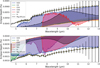 |
Fig. A.3 JWST MIRI simulated spectra for day- (top) and night-side (bottom) of WASP-103b with phase curve observations. Yellow points mark the simulated spectra and with colored areas we show the relative contributions of various species. SiO (in red) as a tracer of refractory elements, represents a promising window into a characterization of thermal inversions in ultra-hot-Jupiters as well as their origin. |
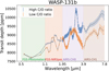 |
Fig. A.4 Simulated Ariel transmission spectra of WASP-131b’s atmosphere. With colors, we distinguish two models with distinct C/O ratios corresponding to different histories of the planet. |
Appendix B Additional figures
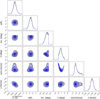 |
Fig. B1 MCMC results of WASP-77 Ab |
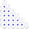 |
Fig. B2 MCMC results of WASP-101b |
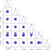 |
Fig. B3 MCMC results of WASP-103b |
 |
Fig. B4 MCMC results of WASP-105b |
 |
Fig. B5 MCMC results of WASP-120b |
 |
Fig. B6 MCMC results of WASP-131b |
 |
Fig. B7 Top: Periodogram of the ASAS-SN g band data of WASP-77 A. We detect the strongest peak with PRot =16.2 d, corresponding to the stellar rotation. Bottom: Phased ASAS-SN data with the detected stellar rotation period |
References
- Addison, B. C., Tinney, C. G., Wright, D. J., et al. 2016, ApJ, 823, 29 [NASA ADS] [CrossRef] [Google Scholar]
- Albrecht, S., Winn, J. N., Carter, J. A., et al. 2011, ApJ, 726, 68 [NASA ADS] [CrossRef] [Google Scholar]
- Albrecht, S., Winn, J. N., Johnson, J. A., et al. 2012, ApJ, 757, 18 [NASA ADS] [CrossRef] [Google Scholar]
- Albrecht, S. H., Marcussen, M. L., Winn, J. N., et al. 2021, ApJ, 916, L1 [NASA ADS] [CrossRef] [Google Scholar]
- Albrecht, S. H., Dawson, R. I., & Winn, J. N. 2022, PASP, 134, 082001 [NASA ADS] [CrossRef] [Google Scholar]
- Al-Refaie, A. F., Changeat, Q., Waldmann, I. P., & Tinetti, G. 2021, ApJ, 917, 37 [NASA ADS] [CrossRef] [Google Scholar]
- Anderson, D. R., Collier Cameron, A., Delrez, L., et al. 2017, A&A, 604, A110 [NASA ADS] [CrossRef] [EDP Sciences] [Google Scholar]
- Attia, O., Bourrier, V., Delisle, J. B., et al. 2023, A&A, 674, A120 [NASA ADS] [CrossRef] [EDP Sciences] [Google Scholar]
- August, P. C., Bean, J. L., Zhang, M., et al. 2023, ApJ, 953, L24 [CrossRef] [Google Scholar]
- Avallone, E. A., Tayar, J. N., van Saders, J. L., et al. 2022, ApJ, 930, 7 [NASA ADS] [CrossRef] [Google Scholar]
- Barnes, J. R., Jeffers, S. V., Anglada-Escudé, G., et al. 2017, MNRAS, 466, 1733 [NASA ADS] [CrossRef] [Google Scholar]
- Barros, S. C. C., Akinsanmi, B., Boué, G., et al. 2022, A&A, 657, A52 [NASA ADS] [CrossRef] [EDP Sciences] [Google Scholar]
- Batalha, N. E., Mandell, A., Pontoppidan, K., et al. 2017, PASP, 129, 064501 [Google Scholar]
- Bate, M. R., Lodato, G., & Pringle, J. E. 2010, MNRAS, 401, 1505 [NASA ADS] [CrossRef] [Google Scholar]
- Batygin, K. 2012, Nature, 491, 418 [NASA ADS] [CrossRef] [Google Scholar]
- Blanco-Cuaresma, S., Soubiran, C., Heiter, U., et al. 2014, A&A, 569, A111 [NASA ADS] [CrossRef] [EDP Sciences] [Google Scholar]
- Bocchieri, A., Mugnai, L. V., Pascale, E., Changeat, Q., & Tinetti, G. 2023, Exp. Astron., 56, 605 [NASA ADS] [CrossRef] [Google Scholar]
- Bohn, A. J., Southworth, J., Ginski, C., et al. 2020, A&A, 635, A73 [NASA ADS] [CrossRef] [EDP Sciences] [Google Scholar]
- Boué, G., Montalto, M., Boisse, I., et al. 2013, A&A, 550, A53 [NASA ADS] [CrossRef] [EDP Sciences] [Google Scholar]
- Bourrier, V., Lovis, C., Beust, H., et al. 2018, Nature, 553, 477 [NASA ADS] [CrossRef] [Google Scholar]
- Bourrier, V., Attia, O., Mallonn, M., et al. 2023, A&A, 669, A63 [NASA ADS] [CrossRef] [EDP Sciences] [Google Scholar]
- Breslau, A., & Pfalzner, S. 2019, A&A, 621, A101 [NASA ADS] [CrossRef] [EDP Sciences] [Google Scholar]
- Brewer, J. M., Fischer, D. A., & Madhusudhan, N. 2017, AJ, 153, 83 [NASA ADS] [CrossRef] [Google Scholar]
- Casasayas-Barris, N., Orell-Miquel, J., Stangret, M., et al. 2021, A&A, 654, A163 [NASA ADS] [CrossRef] [EDP Sciences] [Google Scholar]
- Changeat, Q. 2022, AJ, 163, 106 [CrossRef] [Google Scholar]
- Changeat, Q., Edwards, B., Al-Refaie, A. F., et al. 2022, ApJS, 260, 3 [NASA ADS] [CrossRef] [Google Scholar]
- Charnay, B., Mendonça, J. M., Kreidberg, L., et al. 2022, Exp. Astron., 53, 417 [NASA ADS] [CrossRef] [Google Scholar]
- Chatterjee, S., Ford, E. B., Matsumura, S., et al. 2008, ApJ, 686, 580 [Google Scholar]
- Czesla, S., Lampón, M., Sanz-Forcada, J., et al. 2022, A&A, 657, A6 [NASA ADS] [CrossRef] [EDP Sciences] [Google Scholar]
- Dalal, S., Hébrard, G., Lecavelier des Étangs, A., et al. 2019, A&A, 631, A28 [NASA ADS] [CrossRef] [EDP Sciences] [Google Scholar]
- Dawson, R. I. 2014, ApJ, 790, L31 [NASA ADS] [CrossRef] [Google Scholar]
- Delrez, L., Madhusudhan, N., Lendl, M., et al. 2018, MNRAS, 474, 2334 [NASA ADS] [CrossRef] [Google Scholar]
- Dong, J., & Foreman-Mackey, D. 2023, AJ, 166, 112 [NASA ADS] [CrossRef] [Google Scholar]
- Doyle, L., Cegla, H. M., Anderson, D. R., et al. 2023, MNRAS, 522, 4499 [NASA ADS] [CrossRef] [Google Scholar]
- Dyrek, A., Min, M., Decin, L., et al. 2024, Nature, 625, 51 [Google Scholar]
- Edwards, B., & Tinetti, G. 2022, AJ, 164, 15 [NASA ADS] [CrossRef] [Google Scholar]
- Edwards, B., Mugnai, L., Tinetti, G., Pascale, E., & Sarkar, S. 2019a, AJ, 157, 242 [NASA ADS] [CrossRef] [Google Scholar]
- Edwards, B., Rice, M., Zingales, T., et al. 2019b, Exp. Astron., 47, 29 [NASA ADS] [CrossRef] [Google Scholar]
- Fabrycky, D., & Tremaine, S. 2007, ApJ, 669, 1298 [NASA ADS] [CrossRef] [Google Scholar]
- Fu, G., Espinoza, N., Sing, D. K., et al. 2022, ApJ, 940, L35 [NASA ADS] [CrossRef] [Google Scholar]
- Fulton, B. J., Petigura, E. A., Blunt, S., et al. 2018, PASP, 130, 044504 [NASA ADS] [CrossRef] [Google Scholar]
- Gandhi, S., & Madhusudhan, N. 2019, MNRAS, 485, 5817 [Google Scholar]
- Gao, P., Thorngren, D. P., Lee, E. K. H., et al. 2020, Nat. Astron., 4, 951 [NASA ADS] [CrossRef] [Google Scholar]
- García Muñoz, A., & Schneider, P. C. 2019, ApJ, 884, L43 [Google Scholar]
- Gebek, A., & Oza, A. V. 2020, MNRAS, 497, 5271 [Google Scholar]
- Gillon, M., Anderson, D. R., Collier-Cameron, A., et al. 2014, A&A, 562, L3 [NASA ADS] [CrossRef] [EDP Sciences] [Google Scholar]
- Grant, D., Lewis, N. K., Wakeford, H. R., et al. 2023, ApJ, 956, L29 [Google Scholar]
- Hamer, J. H., & Schlaufman, K. C. 2022, AJ, 164, 26 [NASA ADS] [CrossRef] [Google Scholar]
- Hands, T. O., & Helled, R. 2022, MNRAS, 509, 894 [Google Scholar]
- Haswell, C. A., Fossati, L., Ayres, T., et al. 2012, ApJ, 760, 79 [Google Scholar]
- Hellier, C., Anderson, D. R., Collier Cameron, A., et al. 2014, MNRAS, 440, 1982 [NASA ADS] [CrossRef] [Google Scholar]
- Hellier, C., Anderson, D. R., Collier Cameron, A., et al. 2017, MNRAS, 465, 3693 [NASA ADS] [CrossRef] [Google Scholar]
- Hirano, T., Gaidos, E., Winn, J. N., et al. 2020, ApJ, 890, L27 [NASA ADS] [CrossRef] [Google Scholar]
- Holt, J. R. 1893, A&A, 12, 646 [Google Scholar]
- Iro, N., Bézard, B., & Guillot, T. 2005, A&A, 436, 719 [NASA ADS] [CrossRef] [EDP Sciences] [Google Scholar]
- Kabáth, P., Zák, J., Boffin, H. M. J., et al. 2019, PASP, 131, 085001 [CrossRef] [Google Scholar]
- Kausch, W., Noll, S., Smette, A., et al. 2015, A&A, 576, A78 [NASA ADS] [CrossRef] [EDP Sciences] [Google Scholar]
- Kawashima, Y., Hu, R., & Ikoma, M. 2019, ApJ, 876, L5 [Google Scholar]
- Keating, D., Cowan, N. B., & Dang, L. 2019, Nat. Astron., 3, 1092 [NASA ADS] [CrossRef] [Google Scholar]
- Kempton, E. M. R., Bean, J. L., Louie, D. R., et al. 2018, PASP, 130, 114401 [Google Scholar]
- Khorshid, N., Min, M., & Désert, J. M. 2023, A&A, 675, A95 [NASA ADS] [CrossRef] [EDP Sciences] [Google Scholar]
- Kirk, J., Rackham, B. V., MacDonald, R. J., et al. 2021, AJ, 162, 34 [NASA ADS] [CrossRef] [Google Scholar]
- Kochanek, C. S., Shappee, B. J., Stanek, K. Z., et al. 2017, PASP, 129, 104502 [Google Scholar]
- Kraft, R. P. 1967, ApJ, 150, 551 [Google Scholar]
- Lai, D. 2012, MNRAS, 423, 486 [NASA ADS] [CrossRef] [Google Scholar]
- Lai, D., Foucart, F., & Lin, D. N. C. 2011, MNRAS, 412, 2790 [NASA ADS] [CrossRef] [Google Scholar]
- Lampón, M., López-Puertas, M., Sanz-Forcada, J., et al. 2023, A&A, 673, A140 [NASA ADS] [CrossRef] [EDP Sciences] [Google Scholar]
- Lendl, M., Cubillos, P. E., Hagelberg, J., et al. 2017, A&A, 606, A18 [NASA ADS] [CrossRef] [EDP Sciences] [Google Scholar]
- Line, M. R., Brogi, M., Bean, J. L., et al. 2021, Nature, 598, 580 [NASA ADS] [CrossRef] [Google Scholar]
- Lodders, K., & Fegley, B. 2002, Icarus, 155, 393 [Google Scholar]
- Lomb, N. R. 1976, Ap&SS, 39, 447 [Google Scholar]
- Lothringer, J. D., Rustamkulov, Z., Sing, D. K., et al. 2021, ApJ, 914, 12 [CrossRef] [Google Scholar]
- Lothringer, J. D., Sing, D. K., Rustamkulov, Z., et al. 2022, Nature, 604, 49 [NASA ADS] [CrossRef] [Google Scholar]
- Maciejewski, G., Fernández, M., Aceituno, F., et al. 2018, Acta Astron., 68, 371 [NASA ADS] [Google Scholar]
- Madhusudhan, N., Amin, M. A., & Kennedy, G. M. 2014, ApJ, 794, L12 [Google Scholar]
- Maeder, A. 2009, Physics, Formation and Evolution of Rotating Stars (Berlin: Springer) [Google Scholar]
- Maxted, P. F. L., Anderson, D. R., Collier Cameron, A., et al. 2013, PASP, 125, 48 [NASA ADS] [CrossRef] [Google Scholar]
- McLaughlin, D. B. 1924, ApJ, 60, 22 [Google Scholar]
- Mugnai, L. V., Pascale, E., Edwards, B., Papageorgiou, A., & Sarkar, S. 2020, Exp. Astron., 50, 303 [NASA ADS] [CrossRef] [Google Scholar]
- Mugnai, L. V., Al-Refaie, A., Bocchieri, A., et al. 2021, AJ, 162, 288 [CrossRef] [Google Scholar]
- Mugnai, L. V., Bocchieri, A., & Pascale, E. 2023, J. Open Source Softw., 8, 5348 [NASA ADS] [CrossRef] [Google Scholar]
- Nagler, P. C., Bernard, L., Bocchieri, A., et al. 2022, SPIE Conf. Ser., 12184, 121840V [NASA ADS] [Google Scholar]
- Ohno, K., & Fortney, J. J. 2023, ApJ, 956, 125 [CrossRef] [Google Scholar]
- Oklopčić, A. 2019, ApJ, 881, 133 [Google Scholar]
- Parmentier, V., Line, M. R., Bean, J. L., et al. 2018, A&A, 617, A110 [NASA ADS] [CrossRef] [EDP Sciences] [Google Scholar]
- Patra, K. C., Winn, J. N., Holman, M. J., et al. 2020, AJ, 159, 150 [NASA ADS] [CrossRef] [Google Scholar]
- Peacock, J. A. 1983, MNRAS, 202, 615 [NASA ADS] [Google Scholar]
- Petrovich, C., Muñoz, D. J., Kratter, K. M., et al. 2020, ApJ, 902, L5 [NASA ADS] [CrossRef] [Google Scholar]
- Polman, J., Waters, L. B. F. M., Min, M., et al. 2023, A&A, 670, A161 [NASA ADS] [CrossRef] [EDP Sciences] [Google Scholar]
- Queloz, D., Eggenberger, A., Mayor, M., et al. 2000, A&A, 359, L13 [NASA ADS] [Google Scholar]
- Rathcke, A. D., Buchhave, L. A., Mendonça, J. M., et al. 2023, MNRAS, 522, 582 [NASA ADS] [CrossRef] [Google Scholar]
- Reggiani, H., Schlaufman, K. C., Healy, B. F., et al. 2022, AJ, 163, 159 [NASA ADS] [CrossRef] [Google Scholar]
- Rice, M., Wang, S., Wang, X.-Y., et al. 2022, AJ, 164, 104 [NASA ADS] [CrossRef] [Google Scholar]
- Ricker, G. R., Winn, J. N., Vanderspek, R., et al. 2015, J. Astron. Telesc. Instrum. Syst., 1, 014003 [Google Scholar]
- Rossiter, R. A. 1924, ApJ, 60, 15 [Google Scholar]
- Sánchez-López, A., Lin, L., Snellen, I. A. G., et al. 2022, A&A, 666, L1 [NASA ADS] [CrossRef] [EDP Sciences] [Google Scholar]
- Scargle, J. D. 1982, ApJ, 263, 835 [Google Scholar]
- Sedaghati, E., Jordán, A., Brahm, R., et al. 2023, AJ, 166, 130 [NASA ADS] [CrossRef] [Google Scholar]
- Shi, Y., Wang, W., Zhao, G., et al. 2023, MNRAS, 522, 1491 [NASA ADS] [CrossRef] [Google Scholar]
- Siegel, J. C., Winn, J. N., & Albrecht, S. H. 2023, ApJ, 950, L2 [NASA ADS] [CrossRef] [Google Scholar]
- Skarka, M., Žák, J., Fedurco, M., et al. 2022, A&A, 666, A142 [NASA ADS] [CrossRef] [EDP Sciences] [Google Scholar]
- Smette, A., Sana, H., Noll, S., et al. 2015, A&A, 576, A77 [NASA ADS] [CrossRef] [EDP Sciences] [Google Scholar]
- Smith, P. C. B., Line, M. R., Bean, J. L., et al. 2024, AJ, 167, 110 [NASA ADS] [CrossRef] [Google Scholar]
- Southworth, J., & Evans, D. F. 2016, MNRAS, 463, 37 [NASA ADS] [CrossRef] [Google Scholar]
- Southworth, J., Bohn, A. J., Kenworthy, M. A., et al. 2020, A&A 635, A74 [NASA ADS] [CrossRef] [EDP Sciences] [Google Scholar]
- Spake, J. J., Sing, D. K., Evans, T. M., et al. 2018, Nature, 557, 68 [Google Scholar]
- Tinetti, G., Drossart, P., Eccleston, P., et al. 2018, Exp. Astron., 46, 135 [NASA ADS] [CrossRef] [Google Scholar]
- Tody, D. 1986, SPIE Conf. Ser., 627, 733 [Google Scholar]
- Triaud, A. H. M. J. 2018, in Handbook of Exoplanets, eds. H. J. Deeg, & J. A. Belmonte (Berlin: Springer), 2 [Google Scholar]
- Triaud, A. H. M. J., Gillon, M., Ehrenreich, D., et al. 2015, MNRAS, 450, 2279 [NASA ADS] [CrossRef] [Google Scholar]
- Tsai, S.-M., Lee, E. K. H., Powell, D., et al. 2023, Nature, 617, 483 [CrossRef] [Google Scholar]
- Turner, O. D., Anderson, D. R., Collier Cameron, A., et al. 2016, PASP, 128, 064401 [NASA ADS] [CrossRef] [Google Scholar]
- Turrini, D., Schisano, E., Fonte, S., et al. 2021, ApJ, 909, 40 [Google Scholar]
- Wakeford, H. R., Stevenson, K. B., Lewis, N. K., et al. 2017a, ApJ, 835, L12 [NASA ADS] [CrossRef] [Google Scholar]
- Wakeford, H. R., Visscher, C., Lewis, N. K., et al. 2017b, MNRAS, 464, 4247 [NASA ADS] [CrossRef] [Google Scholar]
- Welbanks, L., & Madhusudhan, N. 2019, AJ, 157, 206 [NASA ADS] [CrossRef] [Google Scholar]
- Wilson, J., Gibson, N. P., Nikolov, N., et al. 2020, MNRAS, 497, 5155 [NASA ADS] [CrossRef] [Google Scholar]
- Woitke, P., Helling, C., Hunter, G. H., et al. 2018, A&A, 614, A1 [NASA ADS] [CrossRef] [EDP Sciences] [Google Scholar]
- Wöllert, M., & Brandner, W. 2015, A&A, 579, A129 [NASA ADS] [CrossRef] [EDP Sciences] [Google Scholar]
- Wong, I., Shporer, A., Zhou, G., et al. 2021, AJ, 162, 256 [NASA ADS] [CrossRef] [Google Scholar]
- Wyttenbach, A., Ehrenreich, D., Lovis, C., et al. 2015, A&A, 577, A62 [NASA ADS] [CrossRef] [EDP Sciences] [Google Scholar]
- Wyttenbach, A., Mollière, P., Ehrenreich, D., et al. 2020, A&A, 638, A87 [EDP Sciences] [Google Scholar]
- Yan, F., & Henning, T. 2018, Nat. Astron., 2, 714 [Google Scholar]
- Žák, J., Kabáth, P., Boffin, H. M. J., et al. 2019, AJ, 158, 120 [CrossRef] [Google Scholar]
- Zhao, L. L., Kunovac, V., Brewer, J. M., et al. 2022, Nat. Astron., 7, 198 [Google Scholar]
Retrieved from https://exoplanetarchive.ipac.cal.tech.edu/
We used the 2D KS test Python implementation available at https://github.com/syrte/ndtest
We used the obtained υ sin i* from the R-M effect as the value from spectroscopy is a combination of several broadening mechanisms (e.g., Triaud et al. 2015) and is therefore not a good indicator of the rotation period of the star.
We note that given the error bars the system is still aligned within just over 2 sigmas.
All Tables
Transmission (TSM) and emission (ESM) spectroscopy metrics for our sample, as defined in Kempton et al. (2018).
All Figures
|
Fig. 1 Rossiter-Mclaughlin effect of WASP-77 Ab observed with HARPS. The observed data points (black) are shown with their error bars, which in this case are smaller than the symbol size. The systemic velocity was removed for better visibility. The red line shows the model that fits the data best, together with 1σ (dark gray) and 3σ (light gray) confidence intervals. |
| In the text | |
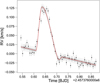 |
Fig. 2 Same as Fig.1 but for WASP-101b. |
| In the text | |
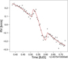 |
Fig. 3 Same as Fig.1 but for WASP-103b. |
| In the text | |
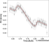 |
Fig. 4 Same as Fig.1 but for WASP-105b. |
| In the text | |
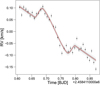 |
Fig. 5 Same as Fig.1 but for WASP-120b. |
| In the text | |
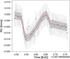 |
Fig. 6 Same as Fig.1 but for WASP-131b. |
| In the text | |
|
Fig. 7 Transmission spectrum for WASP-101b showing a non-detection of any absorbers. The blue dashed lines indicate the position of the Na D2 and D1 lines. We show in cyan a simulated spectrum corresponding to a clear atmosphere model. In red we show a featureless spectrum. The latter model is preferred by a χ2 test. |
| In the text | |
|
Fig. 8 Transmission spectrum for WASP-131 b showing a non-detection of any absorbers. The blue dashed lines indicate the position of the Na D2 and D1 lines. |
| In the text | |
|
Fig. 9 Projected obliquity versus stellar effective temperature. Our targets are plotted with stars. The dashed vertical black line shows the position of the Kraft break. |
| In the text | |
|
Fig. 10 Projected obliquity versus the ratio of the planetary to the stellar mass. Our targets are plotted with stars. |
| In the text | |
|
Fig. A.1 Simulated Ariel emission spectrum of WASP-77Ab’s atmosphere. In orange and blue we show two competing models presented in August et al. (2023). Ariel will be able to distinguish between these two models with high confidence with a single observed eclipse due to its broad wavelength coverage. |
| In the text | |
|
Fig. A.2 Simulated Ariel transmission spectra of WASP-101b’s atmosphere. In orange, we show a model with thick clouds consistent with previous HST data. In blue, we display a model with a clear atmosphere. The colors correspond to the different instruments and channels of Ariel. |
| In the text | |
|
Fig. A.3 JWST MIRI simulated spectra for day- (top) and night-side (bottom) of WASP-103b with phase curve observations. Yellow points mark the simulated spectra and with colored areas we show the relative contributions of various species. SiO (in red) as a tracer of refractory elements, represents a promising window into a characterization of thermal inversions in ultra-hot-Jupiters as well as their origin. |
| In the text | |
|
Fig. A.4 Simulated Ariel transmission spectra of WASP-131b’s atmosphere. With colors, we distinguish two models with distinct C/O ratios corresponding to different histories of the planet. |
| In the text | |
|
Fig. B1 MCMC results of WASP-77 Ab |
| In the text | |
|
Fig. B2 MCMC results of WASP-101b |
| In the text | |
|
Fig. B3 MCMC results of WASP-103b |
| In the text | |
|
Fig. B4 MCMC results of WASP-105b |
| In the text | |
|
Fig. B5 MCMC results of WASP-120b |
| In the text | |
|
Fig. B6 MCMC results of WASP-131b |
| In the text | |
|
Fig. B7 Top: Periodogram of the ASAS-SN g band data of WASP-77 A. We detect the strongest peak with PRot =16.2 d, corresponding to the stellar rotation. Bottom: Phased ASAS-SN data with the detected stellar rotation period |
| In the text | |
Current usage metrics show cumulative count of Article Views (full-text article views including HTML views, PDF and ePub downloads, according to the available data) and Abstracts Views on Vision4Press platform.
Data correspond to usage on the plateform after 2015. The current usage metrics is available 48-96 hours after online publication and is updated daily on week days.
Initial download of the metrics may take a while.