| Issue |
A&A
Volume 694, February 2025
|
|
|---|---|---|
| Article Number | A293 | |
| Number of page(s) | 10 | |
| Section | Planets, planetary systems, and small bodies | |
| DOI | https://doi.org/10.1051/0004-6361/202452124 | |
| Published online | 20 February 2025 | |
PANOPTICON: A novel deep learning model to detect single transit events with no prior data filtering in PLATO light curves
1
Aix Marseille Univ, CNRS, CNES, Institut Origines, LAM,
Marseille,
France
2
Institute for Astronomy, KU Leuven,
Celestijnenlaan 200D bus 2401,
3001
Leuven,
Belgium
3
Université Paris Cité, Université Paris-Saclay, CEA, CNRS, AIM,
91191
Gif-sur-Yvette,
France
★ Corresponding author; hugo.vivien@lam.fr
Received:
5
September
2024
Accepted:
22
January
2025
Aims. To prepare for the analyses of the future PLATO light curves, we develop a deep learning model, PANOPTICON, to detect transits in high precision photometric light curves. Since PLATO’s main objective is the detection of temperate Earth-sized planets around solar-type stars, the code is designed to detect individual transit events. The filtering step, required by conventional detection methods, can affect the transit, which could be an issue for long and shallow transits. To protect the transit shape and depth, the code is also designed to work on unfiltered light curves.
Methods. The PANOPTICON model is based on the Unet family architecture, but it is able to more efficiently extract and combine features of various length scale, leading to a more robust detection scheme. We trained the model on a set of simulated PLATO light curves in which we injected, at the pixel level, planetary, eclipsing binary, or background eclipsing binary signals. We also included a variety of noises in our data, such as granulation, stellar spots, and cosmic rays. We then assessed the capacity of PANOPTICON to detect transits in a separate dataset.
Results. The approach is able to recover 90% of our test population, including more than 25% in the Earth-analog regime, directly in unfiltered light curves. We report that the model also recovers transits irrespective of the orbital period, and it is therefore able to reliably retrieve transits on a single event basis. These figures were obtained when accepting a false alarm rate of 1%. When keeping the false alarm rate low (<0.01%), PANOPTICON is still able to recover more than 85% of the transit signals. Any transit deeper than ~180 ppm is essentially guaranteed to be recovered.
Conclusions. This method is able to recover transits on a single event basis, and it does so with a low false alarm rate. Due to the nature of machine learning, the inference time is minimal, around 0.2 s per light curve of 126 720 points. Thanks to light curves being one dimensional, the model training is also fast, on the order of a few hours per model. This speed in training and inference, coupled with the recovery effectiveness and precision of the model, make this approach an ideal tool to complement or be used ahead of classical approaches.
Key words: techniques: photometric / planets and satellites: detection
© The Authors 2025
 Open Access article, published by EDP Sciences, under the terms of the Creative Commons Attribution License (https://creativecommons.org/licenses/by/4.0), which permits unrestricted use, distribution, and reproduction in any medium, provided the original work is properly cited.
This article is published in open access under the Subscribe to Open model. Subscribe to A&A to support open access publication.
1 Introduction
Out of the currently ∼5700 confirmed planets, close to 3900 have been discovered using transits1. This approach was first successfully used to record the predicted transit of HD209458b in 1999 (Charbonneau et al. 2000), and the first candidate detection came quickly after in 2002 (Udalski et al. 2002) and was later confirmed in 2003 (Konacki et al. 2003). Since then, space-based missions such as CoRoT (Auvergne et al. 2009) and Kepler/K2 (Borucki et al. 2010; Howell et al. 2014) have been designed to acquire the photometry of multiple stars simultaneously, scaling up the ability to detect transits. Additionally, this is the only method allowing direct measurement of certain physical parameters, such as planetary radius, when it is coupled to asteroseismology. To this effect, the second generation of space missions, TESS (Ricker et al. 2015) and CHEOPS (Benz et al. 2021), now provide high-precision photometry of multiple targets.
However, even in high-precision photometry, stellar activity can prevent transit detection and proper characterization. This becomes even more of a problem for long-period planets, where folding the light curve to increase the signal-to-noise ratio might not be an option. So far, the usual approach is to perform a periodicity analysis of the signal, for example with the box least square (BLS; Kovács et al. 2002) or the transit least square2 (TLS; Hippke & Heller 2019) algorithms. For a single transit event, it is mandatory to filter out the stellar activity perfectly to be able to assert the nature of the signal. Currently, using Gaussian processes to fit empirical models has proven effective, but it is quite costly in computation time. Because of the stochastic nature of Gaussian processes, this method requires human supervision in order to avoid affecting the shape and depth of the transit.
Both the prior filtering and the search for a periodic signal set stringent detection limits on the detectable population of exoplanets. For the forthcoming PLATO mission (Rauer et al. 2014, 2024), whose primary goal is the detection and characterization of Earth analogs, this limit is going to become even more prevalent. Indeed the mission’s main challenge will be to detect single transit events that are likely to be Earth-type in order to ascertain the planetary nature of candidates and begin follow-up campaigns as quickly as possible.
The recent and rapid rise of machine learning (ML) methods and its extension, deep learning (DL), for widespread data analysis and its fast paced development offer new opportunities both in applications and methodology. Its use in astrophysics has so far remained somewhat uncommon, despite proving effective at both identification and classification problems, even without prior data filtering. The exoplanet field appears well suited for ML and DL applications, but surprisingly few studies have looked into the possible use cases. Most of the studies so far have focused on vetting of planet candidates in Kepler/K2 (McCauliff et al. 2015; Ansdell et al. 2018; Shallue & Vanderburg 2018; Dattilo et al. 2019), Kepler and TESS (Valizadegan et al. 2022), and NGTS (Armstrong et al. 2018). Fewer still have looked at direct detection: Zucker & Giryes (2018) injected periodic signals in synthetic noisy light curves, and Malik et al. (2022) investigated long-period planets in TESS light curves.
In this work, we present PANOPTICON, a DL model designed to detect single events in unfiltered light curves. The aim of avoiding signal filtering prior to detection is to prevent shallow transits from being phased out in fitted models (as could occur with a Gaussian processes). This approach therefore improves the detection of long-period planets. We trained and tested our approach on simulated PLATO light curves, and we extracted the position of likely threshold crossing events (TCE) in the light curves.
The work is organized as follows: first we describe the architecture of the model in Sect. 2 and our dataset in Sect. 3. We detail our results and performances in Sect. 4. Finally, we present our conclusions in Sect. 5.
2 Deep learning model
In this paper, we present a DL model that is able to identify transit signals in a light curve. This is done by localizing the position of transit events. We do this in the context of the forthcoming ESA PLATO mission, which is designed to determine the frequency of Earth-sized planets orbiting Sun-like stars. We opted for a classifier approach that rates the probability that a transit is occurring at each point of a light curve. This allows our approach to retrieve an arbitrary number of transits in a light curve, including the case of mono-transits. Additionally, we rely on the DL ability to extract and classify features in order to properly identify the events to bypass the filtering process3.
2.1 Architectures
We implemented a custom one-dimensional version of the Unet family: Unet, Unet++, and Unet3+ (Ronneberger et al. 2015; Zhou et al. 2018; Huang et al. 2020). This architecture is a type of fully convolutional neural network that adds successive upsampling layers to the usual contracting networks. By combining the features extracted from the contracting steps with the outputs of the upsampling process, the model can yield a high- resolution output. For our light curves, the output generated acts as a one-to-one map of the input, where each point is classified individually based on the neighboring context.
A Unet model can be seen as an auto-encoder with skip connections between the layers of the encoder part and the decoder part. The encoder extracts contextual information from the input, while the decoder builds the output point by point. During the encoding process, the input is iteratively downsampled, allowing a fixed-size kernel to extract information over a larger window at each step. Then, the decoder iteratively upsamples the output of the encoder, combining it with the features previously extracted at various timescales. The output of the decoder is therefore a segmentation map covering the input point to point, and it allows for precise localization of the object of interest in the input light curve. Moreover, a DL model with skip connections is beneficial, as they have been shown to increase training speed and allow for deeper networks (Drozdzal et al. 2016).
Because this approach is a point-wise detection, it presents a few advantages. First and foremost, it allows any transit in a light curve to be detected individually, as points are classified based on local context. Second, the T0 and duration for an arbitrary number of transits in a given light curve can be extracted. Third, because the output yields a probability, it is possible to define the confidence level depending on the required certainty to extract the TCEs. Finally, because DL builds an internal noise model, there is no need for prior filtering of the light curves. Bypassing this step ensures that no shallow signal will be removed by mistake and simplifies the detection process significantly. The theoretical detection of a transit in a light curve by our model is illustrated in Fig. 1, and the models architectures are given in Figs. A.1, A.2 and A.3.
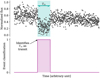 |
Fig. 1 Theoretical input-output scheme of the model. A light curve, normalized between zero and one, is given as input to the model (top panel). We highlight the transit with the blue region. The model returns a classification map for the whole light curve, in purple (bottom panel). |
2.2 Implementation
All of our models are implemented in the PyTorch framework, and the three variants, Unet, Unet++, and Unet3+, are illustrated in Figs. A.1, A.2, and A.3, respectively. The encoder and decoder can be seen as a series of nodes, either extracting features or combining them, respectively. Each node is built on a basic convolution block, illustrated in Fig. 2. This block consists of three basic operations: a convolution, a batch normalization, and a rectified linear unit. An additional, optional, dropout layer can be included at the beginning of the block. The node of the backbone makes use of two consecutive blocks in the cases of Unet and Unet++ and uses a single block for Unet3+.
We identify the nodes of the model as xi, j. The index i corresponds to the depth of the node in the network. It increases with each downsample operation and decreases with each upsample. Conversely, index j tracks the number of upsampling steps to reach a given node. We can therefore easily identify every node in the models. The backbone of the models corresponds to nodes xi,0. Reciprocally, the decoder is made up of the nodes xi,j>0. The backbone is common to all models and can be computed using
 (1)
(1)
where 𝒩 is the operation assigned to the node using the default block, described above. The term 𝒟 corresponds to the downsampling operation (Max Pooling; see Appendix A for details on the operations). The key point of each node is that the length (duration) of the channels is halved, while the number of feature channels is doubled. This is what enables the model to assess the data over multiple scales and efficiently combine the features extracted at each of the previous steps.
Conversely, the decoders of each model can then be computed as follows:
![${x^{i,j > 0}} = \left\{ {\matrix{ {{\cal N}\left( {\left[ {{x^{i,0}},{\cal U}\left( {{x^{i + 1,j - 1}}} \right)} \right]} \right),} \hfill & {{\rm{ Unet }}} \hfill \cr {{\cal N}\left( {\left[ {\left[ {{x^{i,k}}} \right]_{k = 0}^{j,{\cal U}\left( {{x^{i + 1,j - 1}}} \right)}} \right]} \right),} \hfill & {{\rm{ Unet + + }}} \hfill \cr {{\cal N}\left( {\left[ {\matrix{ {\left[ {{\cal N}\left( {{\cal D}\left( {{x^{k,0}}} \right)} \right)} \right]_{k = 0}^{i - 1},} \cr {{\cal N}\left( {{x^{i,0}}} \right),} \cr {\left[ {{\cal N}\left( {{\cal U}\left( {{x^{0,k}}} \right)} \right)} \right]_{k = 0}^{j - 1}} \cr } } \right),} \right.} \hfill & {{\rm{ Unet3 +, }}} \hfill \cr } } \right.$](/articles/aa/full_html/2025/02/aa52124-24/aa52124-24-eq2.png) (2)
(2)
where 𝒟 remains the downsampling operation and 𝒰 is the upsampling operation (transpose convolution for Unet and Unet++ or upsample for Unet3+). The upsampling operation is set up so that it upsamples the data to the same length as the target node. Anything contained within [] is concatenated feature-wise.
The values of the convolution kernel are the trainable parameters of the model. The kernel size is thus key in two aspects: (i) the number of trainable parameters and (ii) the coverage of the signal it offers. A larger kernel can increase the quality of the feature identification at the cost of a longer training time. Additionally, the kernel must be large enough to encompass recognizable features within the signal. To achieve a good balance between feature quality, training time, and feature coverage, we make substantial use of kernel dilation:
 (3)
(3)
where ks is the total length of the kernel, kt is the number of active parameters in the kernel, and d is the dilation factor, namely, the spacing between active points in the kernel. For a default kernel where all active points are next to each other, the dilation factor is one. This allows us to increase the size of the kernel for a fixed number of trainable parameters, at the cost of a lower resolution per feature. The typical kernel size for each architecture is shown in Table 1 for a constant depth of four, and the number of initial feature channels is set to eight. The number of learnable kernel parameters has a strong impact, while each model appears fairly similar. The Unet3+ version displays the smallest number of parameters for a given kernel size, showing the advantage of the full skip connection over the nested skip connections of Unet++.
As described above, the goal of the model is to identify transit events directly within the stellar noise. We therefore limit the model to a binary classification scheme that distinguishes two classes: “continuum” and “event.” Each point in the light curve is assigned a likelihood score of belonging to either the continuum (0) or an event (1). To retrieve the classification, a threshold to separate the two classes needs to be defined. Given the intrinsic class imbalance present within our data, which is caused by the short nature of the transits compared with that of the light curve, it is not guaranteed that setting the threshold to 0.5 will yield the best results (Li et al. 2019). To more effectively constrain the best threshold value, we evaluate the performance of the model for values ranging from 0.05 to 0.95.
Finally, to compare the method’s performance, we trained it over a wide range of parameters, thus leading to multiple versions of the model. This allowed us to compare the aforementioned kernel sizes and coverage of the features. We limited the model to use a binary cross entropy (BCE) loss function, which has proven effective. We used the AdamW optimizer (see Kingma & Ba 2014; Loshchilov & Hutter 2017) with γ = 0.001, β1 = 0.9, and β2 = 0.999. The preliminary test runs showed that a dropout rate of ≈10% yielded the best results, and therefore we set it to this value for all models presented here.
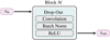 |
Fig. 2 Basic convolution block used in the model. For Unet and Unet++, each node is made up of two consecutive occurrences of this block, while a single one is used for the nodes of Unet3+. The dropout layer encompasses all the other layers in a node, and is used to randomly forgo the computation of feature channels. |
Typical number of parameters for each architecture.
3 Dataset and environment
To prepare a realistic dataset tailored for the PLATO instrument while controlling the astrophysics content of the light curves, we took advantage of the mission end-to-end camera simulator PlatoSim (Jannsen et al. 2024). PlatoSim has been developed to accurately generate realistic images that simulate what will be received from the PLATO satellite. It includes a wide range of instrumental noise sources at different levels: platform; camera, with realistic point spread functions; and detector. With stars that can be observed by a variable number of cameras and the complexity of the instrument, which accommodates 26 cameras on a single optical bench, to control the observation conditions for a given star, we used PlatoSim’s toolkit called PLATOnium. Based on the PLATO input catalog (PIC; Montalto et al. 2021; Nascimbeni et al. 2022), it enables the simulator to be programmed in a user-friendly way. In addition to a realistic representation of the instrument, the other advantage of using PlatoSim is that the signal is injected at the pixel level. While not fundamental to merely test detection capability, the pixel-level injection of the signal is central for later identifying our capacity to sort false positives generated by background eclipsing binaries and bona fide planets.
The initial aim of these simulations was to test algorithms for the filtering of planetary transit candidates in order to prepare the PLATO mission’s exoplanet pipeline, Exoplanet Analysis System (EAS). For the vetting modules of the EAS, this filtering focuses on the suite of tests that could be performed in order to distinguish planetary transits from those caused by eclipsing binaries or background binaries. For the first two cases where the signal is on the target, we could have done this study with data generated with the PLATO solar-like light curve simulator (PSLS; Samadi et al. 2019). Having realistic simulations of background binaries means injecting the signal at the pixel level, hence the use of PlatoSim. It was a project task completely separate from the current study. The dataset is a combination of multiple simulation runs, and each has various internal parameters, leading to the peculiar final distribution. When we started training the ML software, it became clear to us that it would be beneficial to train the software in conditions as close as possible to those of the future instrument and its main scientific objective. Doing so would also provide a good basis for future extensions on classification aspects, for example.
To build our simulated dataset, we chose stars identified in the PIC as potential targets for the prime sample (P1, main sequence stars with Vmag < 11), as the signal-to-noise ratio of these stars enables a detection of an Earth-like planet. We then simulated those stars, including various astrophysical signals: stellar activity effects that include granulation, stochastic oscillations, and stellar spots; exoplanet transits, simulated with BATMAN (Kreidberg 2015); and eclipsing binaries, simulated with ellc (Maxted 2016).
We could thus simulate a target by combining all of these effects to produce either a transiting planet in front of an active star, an eclipsing binary on the target, or an eclipsing binary on a nearby contaminant. All the physical characteristics used to generate the signal (masses, radii, effective temperature, orbital period, ephemerides, eccentricity, rotation period of the star, pulsation frequency, etc.) were also documented and saved.
The prime sample stars can potentially be observed by up to 24 cameras, and the simulator generates the resulting signals and light curve individually for each camera. We included all main effects that are currently implemented in PlatoSim, including the photometry module. At the time when the dataset was generated, only onboard algorithms were implemented by this module. This means that once the full processing chain is complete, the flux is extracted at the pixel level using optimal aperture photometry (see Marchiori et al. 2019). We emphasize that the photometry for bright stars will eventually be derived by point spread function fitting. This prevented us from making use of centroids for the targets. However, since we have control over the simulation, this is a great baseline to evaluate the performance of the method. To reduce the computational cost, the simulations were not performed on a complete PLATO field of view (i.e., simulating full-frame CCD images) but star per star on a CCD subfield of 10 × 10 pixels. We also chose to reduce the cadence from the nominal 25 sec to 1 min and limit the simulations to the first four quarters to cover a one-year time span. We stress that our objective was not to assess the performances of the instrument but to test the ability of our software to detect transit-like events. Depending on the type of simulation (planetary transit, eclipsing binary, number of contaminants, etc.) and the version of the simulator, the computation time for a single target on one quarter and for one camera takes on the order of ≃12 minutes for version 3.6 of PlatoSim, while previous versions took around ≃7 minutes. Finally, still in an effort to save computational resources, we decided to adapt the simulation to the orbital period of the transiting body and did not generate light curves on a given quarter when no transit is expected to occur. As a result, the number of quarters for a given star and a given astrophysical signal is not constant, but it is tailored to the orbital period of the transit signal.
Table 2 gives a summary of the number of different astrophysical signals used in this study. Taking into account the fact that simulations cover a one-year time span and that we do not include quarters where no transit is present, we ended up with a total of 16 094 quarters that were treated as independent light curves. This approach is all the more relevant since the periodic nature of transits does not come into play in our approach and since the light curves were not corrected from any trend, such as instrument aging or even cosmic impacts. We show the resulting distribution of radii and the period of the transiting bodies in Fig. 3.
We further filtered the dataset by removing edge cases where, due to numerical errors, the transits were not visible in the quarters. We also truncated the dataset to remove cases where nonphysical parameters were used to generate light curves. For instance, we removed cases where the stellar radius is greater than 2.5 R⊙ or where the transit depth is is less than 50 ppm. This left us with 14 594 light curves that we randomly split into two datasets: 85% training and 15% validation, that is, 12 405 and 2189 quarters, respectively. The final counts of the signals in the dataset are shown in the right column of Table 2.
Number of simulations per type of signal injected.
4 Performances
While our model returns transits indiscriminately of their planetary or stellar origin, its output is bound to be subsequently analyzed to ascertain the transit parameters. We decided to quantify the limiting factors preventing detection and found that >99% of binary transits are recovered (see Fig. 4), and thus we focus on the model’s results regarding planetary transits.
Evaluation of the performance of the model can be done in two ways: first, by directly evaluating the raw output compared to the desired label and, second, by assessing the ability of the model to detect transit events, or lack thereof. The former is achieved by computing conventional metrics, such as precision, recall, average precision, F1 score, and Jaccard score (or intersection over union). The latter is done by comparing the positions of the ground truths of the events to the positions predicted by the model. While the direct approach allows for a straight-forward evaluation of the model, it also does not reflect its actual ability to detect transits. We therefore focused our estimates on the ability of the model to recover transits as well as its false positive rate (FAR). We deemed a transit to be successfully recovered if an overlap between the prediction and the ground truth exists. The FAR is defined as the fraction of false positives to the total number of predicted events.
The models were trained on A40 GPUs in the in-house cluster of the laboratory. We trained a total of 16 models using the Unet3+ architecture, which we expected to perform the best. We tested multiple initial kernel lengths and trainable parameters, using four or eight initial features, and did this for up to 70 training epochs, using batches of 40 light curves per training pass. To find the best-performing versions of the models, we checked the recovery and FAR performance on the last 20 epochs. We explored two options: a conservative approach that takes the model that has the lowest FAR at the 0.95 confidence threshold and another that finds the version of the models that retrieves the most planets for a constant FAR of 1%. We show a summary of the parameters and their associated results in Table 3.
When taking the models in their conservative regime, we found that our models are able to retrieve more than 80% of our test population, and with a FAR under 0.1%, there is less than one false positive for 1000 predictions. When fixing the FAR to 1%, we found that we are able to retrieve 90% of the planets in our test dataset. These performances demonstrate that this approach is not only viable, but beneficial. The inference mechanism is very fast (∼0.2 seconds per light curve on a CPU), allowing for the processing of large amounts of data, which will be the case for PLATO. In this case, keeping the number of false positives small is key to enabling rapid and accurate processing of the vast amount of light curves.
As highlighted in Table 3, we considered three models that offer the best performances. Model A retrieves the largest fraction of the test population, model B yields a FAR of less than 0.01% while still recovering more than 85% of the planets, and finally model C provides a solid compromise between recovery and FAR. Interestingly, models B and C originate from the same training run and share the same hyper parameters. However, they correspond to two distinct training epochs, leading to different weights in their kernels. We used these models as an illustration for our approach on the population of our dataset. We show in Fig. 5 the effectiveness of model C at 1% FAR at recovering the planets in our test population. The limiting factor for detection that emerges is the depth of the transits and their associated S/N. We computed the S/N by following the approach of Howard et al. (2012):
 (4)
(4)
where δ is the depth of the transit, σCDPP is the combined differential photometric precision, ntr is the number of observed transits, and tdur is the transit duration. While the recovery rate noticeably drops for depths lower than ∼150 ppm (S/N of ∼15), Earth-analogs are detectable by the model. Figure 5c shows the depths of the events, where the expected Earth depth is highlighted as a black vertical line, and neighboring planets are recovered at a rate between 25% and 33%. Additionally, the duration of transits is found to have little impact on the recovery rate (panel d), and crucially, the orbital period also has no impact on transit recovery (panel e). This holds true even for planets with orbital periods longer than a single quarter, indicating that transits are indeed identified on a single event basis. We therefore find that our approach should be able to robustly identify at least 25% of the Earth-analogs.
We subsequently trained the Unet and Unet++ architectures in order to compare their performance relative to the best Unet3+ versions. We find that these alternative models perform slightly worse. Namely, we find that the recovery is lower at equal FAR, especially in the small planets regime. We therefore limited our analysis to the best-performing Unet3+ models.
To better highlight the performance of the models, we illustrate in Fig. 6 the trade-off between the recovery rate and the FAR in a receiver operating characteristic (ROC). We show the three selected models and their compromise, identifying the FAR selected in Table 3. We observed for each case that the number of planets recovered increases with the FAR. Importantly, we find that even for the lowest possible FAR, here model B with <0.01%, a sizable 85.81% of the population is successfully recovered. In Fig. 7, we illustrate the recovery for various depths of transits. The figure clearly shows that the recovery rate rapidly rises above ∼180 ppm, essentially reaching 100% (as also visible in panel c of Fig. 5 for model C).
In addition to the planetary parameters, we highlight the impact stellar activity parameters have on the ability of the model to recover transits in Fig. 8. We found no strong correlation between any activity indicator and our ability to recover transit. Similarly, the rate of false positives and false negatives do not show a clear correlation with the activity of the host star. This indicates that the model is able to internally discern the differences of signal types, even in the cases of signals with similar timescales as those of transits. The only clear limiting factor displaying strong correlation to our detection ability is the S/N of the transit signal.
We illustrate the detection of an Earth-analog signal (RP = 1.11 R⊕, RS = 1.23 R⊙, δ = 83.16 ppm) in Fig. 9 using model C. This single event is recovered with a confidence level of more than 0.65, making this planet detected at a corresponding FAR of less than 0.3%. While not strictly equivalent to the false alarm probability, it is sufficiently analogous to provide insight into the likelihood that this event is a true positive.
We also point out that while training was conducted exclusively on light curves containing transits, this has no bearing on the false positives returned by the model. Since the model in effect operates as a sliding window on the light curve, it only sees a small fraction of a light curve at a given time. Even in the case of our dataset, it in fact had many cases where no transits are present. We illustrate this in Fig. 10, which takes the same light curve as previously shown, but the data have been subdivided into six independent segments. The model was used on each individual segment shown in the figure, and we compared the results to the prediction made on the whole light curve. The only noticeable differences are at the start and end of the segments since this is where the available data are different. Importantly, in the five segments without transits, the model correctly assessed their absence.
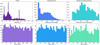 |
Fig. 3 Histograms of the radii and periods of the bodies in our dataset. The left, center, and right columns respectively correspond to the planets, the eclipsing binaries, and the background eclipsing binaries. The three spikes in the planetary population correspond to an erroneous simulation run that did not include the sampling of radii around the central values of the distribution. |
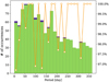 |
Fig. 4 Eclipsing binary transit recovery capabilities. We show the number of recovered transits compared to the total number of binary transits in the dataset, with the corresponding fraction overplotted in orange. The values were found with model B, but all of our models show quasiidentical results for binaries. |
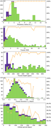 |
Fig. 5 Recovery capabilities of model C. Each panel shows a physical characteristic of our test population, in purple, as well as the fraction recovered by the model, in green. Overlaid in orange is the fraction of the recovered transits per bin. Panel b illustrates that the main cause of missed transits is low S/N. Additionally, panel e shows that the ability to detect transits is not linked to the orbital period, and single transits are therefore detected. |
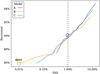 |
Fig. 6 Receiver operating characteristic curve of the three models. The ROC shows the trade-off between the recovery rate of the model and its FAR. Each model’s ROC curve is shown, illustrating the recovery-FAR balance highlighted in Table 3. |
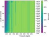 |
Fig. 7 Recovery and FAR of model B. We show the recovered fraction of the transits, binned per depth, depending on the prediction threshold. For each threshold, we also give the FAR resulting from that cutoff value. |
Parameters and performance of every model.
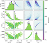 |
Fig. 8 Recovery rate depending on the stellar activity using model A. Each panel of this corner plot illustrates the recovered fraction of planets, for any two stellar activity parameters, while the diagonal shows the recovery for the corresponding parameter. The upper-right corner shows the distribution of the complete dataset. |
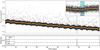 |
Fig. 9 Example detection of an Earth-analog with a depth of 83.16 ppm (S/N of 0.88) using model C. The top panel shows the light curve in black dots, and its one-hour bin is in orange, with the ground truth of the transit shown as a blue span. The bottom panel shows the associated prediction map of the model in purple, with the associated FARs of the model shown as dashed lines. The zoomed-in section highlights the transit, and the model’s predicted position of the transit is indicated with a purple line, extracted at the 1% FAR. |
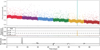 |
Fig. 10 Same example as in Fig. 9, but the light curve is segmented into six individual portions. The sections can be identified by their color. We ran the model on each individual segment and show the resulting predictions with their respective color code. The residuals illustrate the difference between the segmented predictions and the whole light curve prediction. |
5 Discussion
We have presented PANOPTICON, a DL approach designed to detect single transit events in unfiltered PLATO light curves. We trained 16 versions of the model using various hyperparameters to test the robustness of the method and find the bestperforming iterations. We featured three versions of the model corresponding to the best versions for recovery rate (A), lowest FAR (B), and best trade-off between recovery and FAR (C). We trained and tested our method on simulated PLATO light curves generated using the Platosim package. Our dataset contained a total of 14 594 light curves, which we split into training (85%) and testing (15%) subsets.
By fixing the FAR at 1%, we were able to retrieve 90% of the test population in our dataset. Reciprocally, for the model with the lowest FAR, <0.01%, the recovery rate is still of 85.81%. Finally, the model presenting the best mixed characteristics is able to retrieve 89.64% of the population at 1% FAR and has an 85.91% recovery rate at 0.05% FAR. We find that the only limiting factor in detection is the apparent depth (and subsequent S/N), while neither the duration of the event nor the period prevent detection. This means that single transits are indeed recovered successfully without requiring any prior detrending. Additionally, we note that Earth-analog signals, that is, single and shallow transits, are also recovered at a rate between 25% and 30%. Given the ease of use and speed of the method, this range is extremely encouraging and indicates that an even greater recovery of shallow signals is possible. Any signals resulting in a depth greater than 180 ppm are almost systematically recovered, even at a low FAR. Crucially, we report that periodicity is not a factor in the detection process, and even single transits are reliably detected.
We also report that >99% of eclipsing binary transits are also recovered by the model at the same FAR. As it stands, the model does not discriminate between planetary and stellar transit, as not enough information is present in the light curves to reliably allow for such a prediction. However, a version of the model that uses the centroids of the target as additional inputs is considered, which would allow for such a classification scheme to be implemented.
The ability of the model to work without prior filtering of the data significantly simplifies the process of finding and investigating TCEs, for example, by avoiding the drowning of small signals during filtering. Also, with the detection being based on single events, the model is able to reliably detect long-period exoplanets that might only appear once in a dataset. The computation time for detection is essentially instantaneous, making it a very easy tool to use. This is achieved with a training time of around 10 hours per model using our training dataset of 12 405 light curves.
In this paper, we have successfully applied our approach to PLATO data, and work is currently underway to adapt it to TESS light curves. This will enable the characterization of the impact of real-world data rather than simulated data and provide a baseline to compare the abilities of methods with different approaches. Direct comparison to other methods will also be presented in the upcoming release of the results of the PLATO data challenge. To further the capacity of the model, it is possible to develop an approach coupling our model in the high-FAR, high-recovery regime to a vetting model. This would allow for a fair increase of the recall without increasing the FAR. Additionally, when PLATO becomes operational, using the bestperforming model as a baseline to train a dedicated model incorporating annotated real-world data will not only be efficient but ensure a solid foundation.
Acknowledgements
HV and MD acknowledge funding from the Institut Univer- sitaire de France (IUF) that made this work possible, and was also supported by CNES, focused on PLATO. This research made use of the computing facilities operated by the CeSAM data center at the LAM, Marseille, France. We also would like to thank our anonymous referee for their well thought-out comments that improved the clarity of this manuscript.
Appendix A Nomenclature and architectures
In this appendix we give a quick overview of the nomenclature used, as well as the schematics of the model itself.
Channels. We refer to any one-dimensional signal as a channel. Depending on the nature of the data, the channels are considered to be of different type. For example, the input light curve is a data channel, and the output of the first node consists of Ninit feature channels.
Convolution. In the context of deep learning, a convolution layer contains, in fact, multiple convolution kernels. These are used to combine multiple channels together, where the number of input and output channels are set hyper-parameters. In the backbone of the model, the convolutions are set-up to increase the number of channels, while in the decoder they reduce the number of channels until the desired output dimensionality is reached.
Batch normalization. Originally described in Ioffe & Szegedy (2015), this operation is designed to increase model training speeds by re-scaling each training mini-batch. The normalization is computed such that any data channel has a fixed mean and variance, leading to more stability during training. Note that this layer also includes 2 learnable parameters per data channel, that allows for each channel to be treated individually.
ReLU. The rectified linear unit is a type of activation function, which simply returns the max(0, x) of an input x. This simple but important steps drastically reduces the vanishing gradient problem during back-propagation.
Dropout. The dropout operation randomly zeroes out certain channels during inference, nullifying their gradients. This allows for more independence between feature channels to be learned during the back-propagation step. This not only improves the detection capabilities, but also reduces computer resources usage by removing redundant computations.
Max pooling. This operation is used as a downsampling layer for the data. It does so by returning the maximum value within its kernel length. In our case, we set the kernel of length and stride to 2, resulting in the halving of the length of the channels.
Transpose convolution. Working as a counterpart to the convolution, this operation constructs its output by convolving a padded version of the input. For the exact methodology relating to convolution arithmetic, see Dumoulin & Visin (2016).
Upsample. Computation of a channel with more points than the input. In the PyTorch framework, this operation is implemented with a variety of method, and in this work we use a simple linear scheme to compute the new points.
Concatenation. The concatenation procedure is such that the 1-dimensional channels are concatenated along the features axis. For example, when concatenating N channels of length L, the output has dimension [N, L].
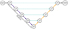 |
Fig. A.1 Architecture of Unet presented here with a depth of four. The architecture makes use of downsampling and upsampling steps of the original input. This allows the extraction of features of various sizes, and recombining them during decoding via the plain skip connections. Solid purple (resp. orange) arrows represent the downsampling (resp. upsampling), and the dashed lines are the skip connections between the nodes. |
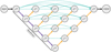 |
Fig. A.2 Architecture of Unet++ of the same depth as Fig. A.1. This version introduces a more complex recombination during decoding. Each encoding level is upsampled individually and combined in nested dense skip connections. This gives a better merging of various feature sizes when creating the output. |
 |
Fig. A.3 Architecture of Unet3+ of the same depth as Figs. A.1 and A.2. The skip connections are here not upsampled for each encoder level, but are included directly when computing the decoder levels, and merged with previous decoder levels. This creates a simpler decoding process, limiting the number of free parameters compared to Unet++, as there are no in between convolution layer. |
References
- Ansdell, M., Ioannou, Y., Osborn, H. P., et al. 2018, ApJ, 869, L7 [NASA ADS] [CrossRef] [Google Scholar]
- Armstrong, D. J., Günther, M. N., McCormac, J., et al. 2018, MNRAS, 478, 4225 [NASA ADS] [CrossRef] [Google Scholar]
- Auvergne, M., Bodin, P., Boisnard, L., et al. 2009, A&A, 506, 411 [NASA ADS] [CrossRef] [EDP Sciences] [Google Scholar]
- Benz, W., Broeg, C., Fortier, A., et al. 2021, Exp. Astron., 51, 109 [Google Scholar]
- Borucki, W. J., Koch, D., Basri, G., et al. 2010, Science, 327, 977 [Google Scholar]
- Charbonneau, D., Brown, T. M., Latham, D. W., & Mayor, M. 2000, ApJ, 529, L45 [Google Scholar]
- Dattilo, A., Vanderburg, A., Shallue, C. J., et al. 2019, AJ, 157, 169 [NASA ADS] [CrossRef] [Google Scholar]
- Drozdzal, M., Vorontsov, E., Chartrand, G., Kadoury, S., & Pal, C. 2016, in International Workshop on Deep Learning in Medical Image Analysis, International Workshop on Large-scale Annotation of Biomedical Data and Expert Label Synthesis (Springer), 179 [Google Scholar]
- Dumoulin, V., & Visin, F. 2016, arXiv e-prints [arXiv:1603.07285] [Google Scholar]
- Hippke, M., & Heller, R. 2019, A&A, 623, A39 [NASA ADS] [CrossRef] [EDP Sciences] [Google Scholar]
- Howard, A. W., Marcy, G. W., Bryson, S. T., et al. 2012, ApJS, 201, 15 [Google Scholar]
- Howell, S. B., Sobeck, C., Haas, M., et al. 2014, PASP, 126, 398 [Google Scholar]
- Huang, H., Lin, L., Tong, R., et al. 2020, arXiv e-prints [arXiv:2004.08790] [Google Scholar]
- Ioffe, S., & Szegedy, C. 2015, arXiv e-prints [arXiv:1502.03167] [Google Scholar]
- Jannsen, N., De Ridder, J., Seynaeve, D., et al. 2024, A&A, 681, A18 [NASA ADS] [CrossRef] [EDP Sciences] [Google Scholar]
- Kingma, D. P., & Ba, J. 2014, arXiv e-prints [arXiv:1412.6980] [Google Scholar]
- Konacki, M., Torres, G., Jha, S., & Sasselov, D. D. 2003, Nature, 421, 507 [NASA ADS] [CrossRef] [Google Scholar]
- Kovács, G., Zucker, S., & Mazeh, T. 2002, A&A, 391, 369 [Google Scholar]
- Kreidberg, L. 2015, PASP, 127, 1161 [Google Scholar]
- Li, Z., Kamnitsas, K., & Glocker, B. 2019, arXiv e-prints [arXiv:1907.10982] [Google Scholar]
- Loshchilov, I., & Hutter, F. 2017, arXiv e-prints [arXiv:1711.05101] [Google Scholar]
- Malik, S. A., Eisner, N. L., Lintott, C. J., & Gal, Y. 2022, arXiv e-prints [arXiv:2211.06903] [Google Scholar]
- Marchiori, V., Samadi, R., Fialho, F., et al. 2019, A&A, 627, A71 [NASA ADS] [CrossRef] [EDP Sciences] [Google Scholar]
- Maxted, P. F. L. 2016, A&A, 591, A111 [NASA ADS] [CrossRef] [EDP Sciences] [Google Scholar]
- McCauliff, S. D., Jenkins, J. M., Catanzarite, J., et al. 2015, ApJ, 806, 6 [NASA ADS] [CrossRef] [Google Scholar]
- Montalto, M., Piotto, G., Marrese, P. M., et al. 2021, A&A, 653, A98 [NASA ADS] [CrossRef] [EDP Sciences] [Google Scholar]
- Nascimbeni, V., Piotto, G., Börner, A., et al. 2022, A&A, 658, A31 [NASA ADS] [CrossRef] [EDP Sciences] [Google Scholar]
- Rauer, H., Catala, C., Aerts, C., et al. 2014, Exp. Astron., 38, 249 [Google Scholar]
- Rauer, H., Aerts, C., Cabrera, J., et al. 2024, arXiv e-prints [arXiv:2406.05447] [Google Scholar]
- Ricker, G. R., Winn, J. N., Vanderspek, R., et al. 2015, J. Astron. Telesc. Instrum. Syst., 1, 014003 [Google Scholar]
- Ronneberger, O., Fischer, P., & Brox, T. 2015, arXiv e-prints [arXiv:1505.04597] [Google Scholar]
- Samadi, R., Deru, A., Reese, D., et al. 2019, A&A, 624, A117 [NASA ADS] [CrossRef] [EDP Sciences] [Google Scholar]
- Shallue, C. J., & Vanderburg, A. 2018, AJ, 155, 94 [NASA ADS] [CrossRef] [Google Scholar]
- Udalski, A., Zebrun, K., Szymanski, M., et al. 2002, Acta Astron., 52, 115 [Google Scholar]
- Valizadegan, H., Martinho, M. J. S., Wilkens, L. S., et al. 2022, ApJ, 926, 120 [NASA ADS] [CrossRef] [Google Scholar]
- Zhou, Z., Mahfuzur Rahman Siddiquee, M., Tajbakhsh, N., & Liang, J. 2018, arXiv e-prints [arXiv:1807.10165] [Google Scholar]
- Zucker, S., & Giryes, R. 2018, AJ, 155, 147 [NASA ADS] [CrossRef] [Google Scholar]
Data from https://exoplanet.eu/
The v1.0.0 of the code is available at https://github.com/At0micBee/Panopticon/tree/v1.0.0
All Tables
All Figures
|
Fig. 1 Theoretical input-output scheme of the model. A light curve, normalized between zero and one, is given as input to the model (top panel). We highlight the transit with the blue region. The model returns a classification map for the whole light curve, in purple (bottom panel). |
| In the text | |
|
Fig. 2 Basic convolution block used in the model. For Unet and Unet++, each node is made up of two consecutive occurrences of this block, while a single one is used for the nodes of Unet3+. The dropout layer encompasses all the other layers in a node, and is used to randomly forgo the computation of feature channels. |
| In the text | |
|
Fig. 3 Histograms of the radii and periods of the bodies in our dataset. The left, center, and right columns respectively correspond to the planets, the eclipsing binaries, and the background eclipsing binaries. The three spikes in the planetary population correspond to an erroneous simulation run that did not include the sampling of radii around the central values of the distribution. |
| In the text | |
|
Fig. 4 Eclipsing binary transit recovery capabilities. We show the number of recovered transits compared to the total number of binary transits in the dataset, with the corresponding fraction overplotted in orange. The values were found with model B, but all of our models show quasiidentical results for binaries. |
| In the text | |
|
Fig. 5 Recovery capabilities of model C. Each panel shows a physical characteristic of our test population, in purple, as well as the fraction recovered by the model, in green. Overlaid in orange is the fraction of the recovered transits per bin. Panel b illustrates that the main cause of missed transits is low S/N. Additionally, panel e shows that the ability to detect transits is not linked to the orbital period, and single transits are therefore detected. |
| In the text | |
|
Fig. 6 Receiver operating characteristic curve of the three models. The ROC shows the trade-off between the recovery rate of the model and its FAR. Each model’s ROC curve is shown, illustrating the recovery-FAR balance highlighted in Table 3. |
| In the text | |
|
Fig. 7 Recovery and FAR of model B. We show the recovered fraction of the transits, binned per depth, depending on the prediction threshold. For each threshold, we also give the FAR resulting from that cutoff value. |
| In the text | |
|
Fig. 8 Recovery rate depending on the stellar activity using model A. Each panel of this corner plot illustrates the recovered fraction of planets, for any two stellar activity parameters, while the diagonal shows the recovery for the corresponding parameter. The upper-right corner shows the distribution of the complete dataset. |
| In the text | |
|
Fig. 9 Example detection of an Earth-analog with a depth of 83.16 ppm (S/N of 0.88) using model C. The top panel shows the light curve in black dots, and its one-hour bin is in orange, with the ground truth of the transit shown as a blue span. The bottom panel shows the associated prediction map of the model in purple, with the associated FARs of the model shown as dashed lines. The zoomed-in section highlights the transit, and the model’s predicted position of the transit is indicated with a purple line, extracted at the 1% FAR. |
| In the text | |
|
Fig. 10 Same example as in Fig. 9, but the light curve is segmented into six individual portions. The sections can be identified by their color. We ran the model on each individual segment and show the resulting predictions with their respective color code. The residuals illustrate the difference between the segmented predictions and the whole light curve prediction. |
| In the text | |
|
Fig. A.1 Architecture of Unet presented here with a depth of four. The architecture makes use of downsampling and upsampling steps of the original input. This allows the extraction of features of various sizes, and recombining them during decoding via the plain skip connections. Solid purple (resp. orange) arrows represent the downsampling (resp. upsampling), and the dashed lines are the skip connections between the nodes. |
| In the text | |
|
Fig. A.2 Architecture of Unet++ of the same depth as Fig. A.1. This version introduces a more complex recombination during decoding. Each encoding level is upsampled individually and combined in nested dense skip connections. This gives a better merging of various feature sizes when creating the output. |
| In the text | |
|
Fig. A.3 Architecture of Unet3+ of the same depth as Figs. A.1 and A.2. The skip connections are here not upsampled for each encoder level, but are included directly when computing the decoder levels, and merged with previous decoder levels. This creates a simpler decoding process, limiting the number of free parameters compared to Unet++, as there are no in between convolution layer. |
| In the text | |
Current usage metrics show cumulative count of Article Views (full-text article views including HTML views, PDF and ePub downloads, according to the available data) and Abstracts Views on Vision4Press platform.
Data correspond to usage on the plateform after 2015. The current usage metrics is available 48-96 hours after online publication and is updated daily on week days.
Initial download of the metrics may take a while.