| Issue |
A&A
Volume 665, September 2022
|
|
|---|---|---|
| Article Number | A11 | |
| Number of page(s) | 19 | |
| Section | Planets and planetary systems | |
| DOI | https://doi.org/10.1051/0004-6361/202141640 | |
| Published online | 01 September 2022 | |
Transit least-squares survey
IV. Earth-like transiting planets expected from the PLATO mission
1
Max-Planck-Institut für Sonnensystemforschung,
Justus-von-Liebig-Weg 3,
37077
Göttingen, Germany
e-mail: This email address is being protected from spambots. You need JavaScript enabled to view it.
2
Institute of Planetary Research, German Aerospace Center,
Rutherfordstrasse 2,
12489
Berlin, Germany
e-mail: This email address is being protected from spambots. You need JavaScript enabled to view it.
3
LESIA, Observatoire de Paris, Université PSL, CNRS, Sorbonne Université, Université Paris Diderot, Sorbonne Paris Cité,
5 place Jules Janssen,
92195
Meudon, France
e-mail: This email address is being protected from spambots. You need JavaScript enabled to view it.
Received:
25
June
2021
Accepted:
20
June
2022
Abstract
In its long-duration observation phase, the PLATO satellite (scheduled for launch in 2026) will observe two independent, non-overlapping fields, nominally one in the northern hemisphere and one in the southern hemisphere, for a total of four years. The exact duration of each pointing will be determined two years before launch. Previous estimates of PLATO’s yield of Earth-sized planets in the habitable zones (HZs) around solar-type stars ranged between 6 and 280. We use the PLATO Solar-like Light curve Simulator (PSLS) to simulate light curves with transiting planets around bright (mV ≤ 11) Sun-like stars at a cadence of 25 s, roughly representative of the >15 000 targets in PLATO’s high-priority P1 sample (mostly F5-K7 dwarfs and subdwarfs). Our study includes light curves generated from synchronous observations of 6, 12, 18, and 24 of PLATO’s 12 cm aperture cameras over both 2 and 3yr of continuous observations. Automated detrending is done with the Wotan software, and post-detrending transit detection is performed with the transit least-squares (TLS) algorithm. Light curves combined from 24 cameras yield true positive rates (TPRs) near unity for planets ≥1.2 R⊕ with two transits. If a third transit is in the light curve, planets as small as 1 R⊕ are recovered with TPR ~ 100%. We scale the TPRs with the expected number of stars in the P1 sample and with modern estimates of the exoplanet occurrence rates and predict the detection of planets with 0.5 R⊕ ≤ Rp ≤ 1.5 R⊕ in the HZs around F5-K7 dwarf stars. For the long-duration observation phase (2yr + 2yr) strategy we predict 11–34 detections, and for the (3 yr + 1 yr) strategy we predict 8–25 discoveries. These estimates neglect exoplanets with monotransits, serendipitous detections in stellar samples P2–P5, a dedicated removal of systematic effects, and a possible bias of the P1 sample toward brighter stars and high camera coverage due to noise requirements. As an opposite effect, Earth-sized planets might typically exhibit transits around P1 sample stars shallower than we have assumed since the P1 sample will be skewed toward spectral types earlier than the Sun-like stars assumed in our simulations. Moreover, our study of the effects of stellar variability on shallow transits of Earth-like planets illustrates that our estimates of PLATO’s planet yield, which we derive using a photometrically quiet star similar to the Sun, must be seen as upper limits. In conclusion, PLATO’s detection of about a dozen Earth-sized planets in the HZs around solar-type stars will mean a major contribution to this as yet poorly sampled part of the exoplanet parameter space with Earth-like planets.
Key words: methods: data analysis / occultations / planets and satellites: detection / stars: solar-type / techniques: photometric
© R. Heller et al. 2022
 Open Access article, published by EDP Sciences, under the terms of the Creative Commons Attribution License (https://creativecommons.org/licenses/by/4.0), which permits unrestricted use, distribution, and reproduction in any medium, provided the original work is properly cited.
This article is published in open access under the Subscribe-to-Open model.
Open Access funding provided by Max Planck Society.
1 Introduction
The science of extrasolar planets is driven to a large extent by transiting planets, that is, planets passing in front of their host stars once every orbit as seen from Earth (Charbonneau et al. 2000). In fact, most of the planets known beyond the Solar System have been found via the transit method in the long-term stellar light curves from space-based missions, starting with 37 planets and brown dwarfs from the CoRoT mission (2009–2013; Auvergne et al. 2009; Deleuil et al. 2018), over 2700 exo-planets and about 2100 candidates yet to be validated1 from the Kepler primary mission (2009–2013; Borucki et al. 2010), more than 500 transiting planets and almost 1000 candidates1 from the extended Kepler mission, called K2 (2014–2018; Howell et al. 2014), and the addition of over 200 exoplanets1 discovered with the ongoing TESS mission (since 2018; Ricker et al. 2015).
Despite the rapid increase in the number of known planets by about three orders of magnitude within three decades (Heller & Kiss 2019), it remains extremely challenging to find Earth-sized planets in Earth-like orbits around Sun-like stars. As a result, it is hard to constrain their occurrence rates, even with four years of continuous observations from the Kepler primary mission (Mulders et al. 2019; Hsu et al. 2019; Kunimoto & Matthews 2020; Bryson et al. 2021). The key challenges for Kepler were the small number of transits of these planets (Kepler required three), a systematic effect in the Kepler data known as the rolling-band effect (Van Cleve & Caldwell 2016; Thompson et al. 2018; Bryson et al. 2021), and the fact that stars are more variable than predicted via the scaling of the solar power spectrum (Gilliland et al. 2011, 2015). Even detections of super-Earth-sized planets in one-year orbits around Sun-like stars such as Kepler-452b (Jenkins et al. 2015) and KOI-456.04 (Heller et al. 2020) have been challenging due to these caveats (Mullally et al. 2018).
The science objective of the PLATO mission (Rauer et al. 2014), with an expected launch in December 2026, is to find terrestrial planets in the habitable zones (HZs; Kasting et al. 1993) of solar-like stars and to determine their bulk properties2. To achieve this goal, PLATO’s 24 normal cameras3 will observe over 15 000 bright (mV ≤ 11) dwarfs and subgiants of spectral types F5-K7 with a precision of 50ppm in 1hr of integration (Montalto et al. 2021). This subset of the hundreds of thousands of stars that PLATO will observe in total is referred to as the P1 stellar sample, and it will be given the highest priority of all the samples. Over 5000 stars with mV ≤ 11 will have their bulk densities measured using asteroseismology. The P1 sample will be observed during the long-duration observation phase, which will take a total of four years, and be compiled from the northern PLATO field (NPF) and the southern PLATO field (SPF). Figure 1 shows the distribution of the PLATO fields that include the preliminary NPF and SPF on the celestial plane. A more up-to-date definition of these fields, which are referred to as Long-duration Observation Phase North 1 (LOPN1) and Long-duration Observation Phase South 1 (LOPS1), is given in (Nascimbeni et al. 2022).
The Gaia mission has already provided highly accurate parallax and optical photometry measurements of essentially all main-sequence stars with mV ≲ 20 (Gaia Collaboration 2016, 2021). In combination with effective temperature measurements from PLATO’s ground-based high-resolution spectroscopy follow-up, stellar radii will be determined with an accuracy of 1–2%, masses will be inferred with an accuracy of 10%, and ages will be estimated using stellar evolution models with an accuracy of 10% for over 5000 F5-K7 stars.
The PLATO Definition Study Report predicted PLATO’s yield of Earth-sized transiting planets in the HZ around Sunlike stars to range between 6 and 280. The details depend on PLATO’s observing strategy, that is, whether it observes its two independent long-duration observation phase fields for 2 yr each (the 2yr + 2yr scenario) or one field for 3yr and the other one for 1 yr (the 3 yr + 1 yr scenario). These yield predictions were derived with exoplanet occurrence rates that were still very uncertain at the time (Fressin et al. 2013). The PLATO Definition Study Report considered an occurrence rate of planets in the HZ with radii smaller than two Earth radii (Rp < 2 R⊕) of between 2 and 100%, with a nominal value of 40%. The most recent and comprehensive statistical analysis of the completeness and reliability of the Kepler survey by Bryson et al. (2021) suggests that the occurrence rate of planets with 0.5 R⊕ ≤ Rp ≤ 1.5 R⊕ and orbital periods between 340 d and 760 d (the conservative HZ; Kopparapu et al. 2014) around G and K dwarf stars is closer to 60%. Moreover, previous yield predictions for PLATO were necessarily based on analytical estimates of the expected signal-to-noise ratio (S/N) of the transits and taking the activity of Sun-like stars observed with Kepler into account.
With the launch date of the PLATO mission approaching, great progress has been made in the simulation of light curves that can be expected from PLATO. The PLATOSim software (Marcos-Arenal et al. 2014) provides end-to-end simulations from the charge-coupled device (CCD) level to the final light curve product. The PLATO Solar-like Light curve Simulator (PSLS), following a much more pragmatic and computationally efficient approach, allows simulations of a large number of PLATO-like light curves with realistic treatment of the main sources of astrophysical and systematic noise (Samadi et al. 2019). As for transit detection, the Wotan detrending software for stellar light curves has been optimized with a particular focus on the preservation of exoplanet transits (Hippke et al. 2019). This optimization was achieved based on extended benchmarking tests invoking detrending and transit searches in light curves from the Kepler primary mission, K2, and TESS. Finally, the release of the transit least-squares (TLS) software provides enhanced detection sensitivity for small planets over the traditional box least-squares (BLS) algorithm (Kovács et al. 2002). As shown by Hippke & Heller (2019), for a parameterization of TLS and BLS that produces a false positive rate (FPR) of 1% in a search for transits of Earth-like planets around Sun-like stars, the true positive rate (TPR) of TLS is about 93%, while it is roughly 76% for BLS. This sensitivity gain of TLS over BLS will be vital for PLATO’s discovery of Earth-sized planets in the HZs around Sun-like stars.
The key objectives of this paper are to update PLATO’s expected yield of Earth-like planets in the HZs around Sun-like stars and to test if currently available transit search software would be sufficient to find these planets in PLATO data and enable PLATO to achieve its science objectives.
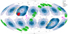 |
Fig. 1 Provisional pointing of PLATO’s northern (NPF) and southern (SPF) long-duration phase fields in an all-sky Aitoff projection using Galactic coordinates (an updated version is available in Nascimbeni et al. 2022). The centers of the NPF and SPF are covered by 24 cameras (light blue). Increasingly darker blue tones refer to a coverage by 18, 12, and 6 cameras, respectively. Provisional step-and-stare field pointings (STEP01 – STEP10) use dark blue tones for an overlap of 24 cameras and lighter blue tones for 18, 12, and 6 cameras, respectively. The fields of CoRoT (pink), Kepler (red), K2 (green), and the TESS continuous viewing zone (yellow) are also shown. |
2 Methods
The principal approach of our study is as follows. We used PSLS to simulate a sufficiently large number (~10 000) of PLATOlike light curves for Sun-like stars, including stellar variability and systematic effects, some with transits of Earth-like planets, some without any transits. Then we used Wotan to automatically detrend the light curves from any stellar and systematic variability while preserving any possible transit signals. To infer the detectability of the injected transits as well as the corresponding false alarm probability, we searched for the transits using TLS. A comparison of the injected signals with our results from the recovery tests then yielded the true and FPRs, which we scaled with literature values for the planet occurrence rates to predict the number of Earth-like planets to be detected with PLATO.
2.1 PLATO Solar-Like Light Curve Simulator
Our analysis starts with the generation of synthetic PLATO-like light curves with the publicly available4 PSLS (v1.3) Python software (Samadi et al. 2019). PSLS simulates Poisson noise characteristic for a given stellar magnitude, instrumental effects, systematic errors, and stellar variability.
In a first step, PSLS reads the input YAML file to simulate the stellar signal in Fourier space. Then random noise is added (Anderson et al. 1990) to mimic the stochastic behavior of the signal and finally the signal is transformed back into the time domain to generate the light curve.
The stellar oscillation spectrum is computed as a sum of resolved and unresolved differential modes, which are modeled with specific Lorentzian profiles in the power spectral density space (Berthomieu et al. 2001; Samadi et al. 2019). The mode frequencies, mode heights, and mode line widths for main-sequence and subgiant stars are precomputed with the Aarhus adiabatic pulsation package (ADIPLS) (Christensen-Dalsgaard 2008). Stellar activity phenomena such as magnetic activity (star spots), p-mode oscillations, and granulation lead to time-dependent variability for the disk-integrated flux of a solar-like star. The stellar activity component is simulated in PSLS with a Lorentzian profile in frequency space, and it includes an amplitude (σA, subscript “A” referring to activity) and a characteristic timescale (τA), both of which can be adjusted in PSLS (Samadi et al. 2019). Stellar granulation, caused by convection currents of plasma within the star’s convective zone, occurs on a scale from granules the size of ~0.5 Mm (~0.08 R⊕) to supergranules with diameters of ~16 Mm (~2.5 R⊕), all of which appear stochastically over time (Morris et al. 2020). Granulation is simulated in PSLS using the two pseudo-Lorentzian functions with characteristic timescales τ1,2 (Samadi et al. 2019).
Systematic errors of the PLATO instrument are simulated in PSLS using the Plato Image Simulator (PIS), developed at the Laboratoire d’études spatiales et d’instrumentation en astrophysique (LESIA) at the Observatoire de Paris. PIS models different sources of noise and other perturbations, like photon noise, readout noise, smearing, long-term drift, satellite jitter, background signal, intra-pixel response nonuniformity, pixel response nonuniformity, digital saturation (Janesick 2001; Marcos-Arenal et al. 2014), charge diffusion (Lauer 1999), and charge transfer inefficiency (Short et al. 2013). In our simulations we used the beginning-of-life setup tables for systematics, where charge transfer inefficiency is not included in simulating systematics. We also turned off jitter in PIS as it demands substantial amounts of CPU time. Furthermore, according to the PLATO Study Definition Report, the pointing errors are expected to be sufficiently low that they will be negligible to the overall noise (see also Marchiori et al. 2019). Light curves for the P1 sample will not be extracted from aperture masks but from the downloaded imagettes using the point-spread function fitting method. The resulting systematic effects, including jumps in the light curves at the quarterly repositioning of the stars on the PLATO CCDs after satellite rotation, are properly taken into account in PSLS.
Finally, planetary transits can be automatically simulated in PSLS data using the Mandel & Agol (2002) model. The actual implementation in PSLS is based on the Python code of Ian Crossfield5. PSLS users can specify the transit parameters, including the planet radius (Rp), the orbital period (P), the planet semimajor axis (a), and the orbital inclination. Transits assume a quadratic limb darkening law as per Mandel & Agol (2002), and the two quadratic limb darkening coefficients of the star can be manually adjusted.
For all our simulations, we chose a solar-type star with solar radius and mass and with Sun-like stellar activity to represent the expected 15 000 to 20 000 F5-K7 stars in the P1 sample. As for the amplitude and characteristic timescale of stellar photometric activity, we assumed activity parameters close to those of 16 Cyg B, that is, σA = 20 ppm and τA = 0.27 d. This is similar to the values used in the default parameterization of the PSLS YAML input file, as described in Samadi et al. (2019, Appendix A therein). 16 Cyg B is a solar-type oscillating main-sequence star, for which stellar activity, asteroseismology, and rotation periods have been well constrained using Kepler data (Davies et al. 2015). In Appendix C we examine the effects of different levels of stellar variability on transit detection with PLATO.
The resulting PSLS light curves are derived as averages from 6, 12, 18, or 24 light curves (corresponding to the number of cameras) and have a cadence of 25 s, representative of the data that will be extracted for the P1 sample. For reference, a PSLS light curve worth of 2yr (3yr) of simulated observations contains about 2.5 (3.7) million data points.
2.2 Light Curve Detrending with Wōtan
Wōtan is a publicly available6 Python software for the detrending of stellar light curves under optimized preservation of exoplanet transit signatures (Hippke et al. 2019). The key value of Wōtan is in its removal of instrumental and stellar variability from light curves to prepare them for transit searches. Woōtan features many different detrending methods. Among all these detrending filters, Hippke et al. (2019) identified the biweight method as the optimal choice in most cases.
We thus use the biweight method in this work with a window size of three times the expected maximum transit duration, as suggested by Hippke et al. (2019), to preserve the transit signatures while removing any other type of variability from the simulated light curves from PSLS. It is worth noting that while we restrict our search to transits of planets in Earth-like orbits and, hence, Earth-like transit durations, in an unrestricted search for transits of different durations the window size of the detrending algorithm would need to be adapted accordingly. Wotan’s treatment of jumps in the PSLS light curves is described in Sect. 4.3.
2.3 Transit Least-Squares
The transit search is executed with the publicly available7 TLS algorithm (Hippke & Heller 2019). TLS is optimized for finding small planets. The principal sensitivity gain over the BLS algorithm (Kovács et al. 2002) is in TLS’s accurate modeling of the planetary ingress and egress and stellar limb-darkening. The template of TLS’s transit search function is parameterized by two limb darkening coefficients required to feed the analytical solution for the light curve with a quadratic limb darkening law (Mandel & Agol 2002).
TLS finds the minimum χ2 value for a range of trial orbital periods (P), transit times t0, and transit durations d. The orbital eccentricity is assumed to be zero, but the transit sequence of planets in highly eccentric orbits are typically found with TLS as long as the transits are periodic. TLS does not fit for transit timing variations (TTVs), but transits are usually recovered as long as the TTV amplitude is smaller than the transit duration.
The key search metric for TLS is the signal detection efficiency (SDE), which is a measure for the significance of the χ2 minimum compared to the surrounding χ2 landscape as a function of the period. Hippke & Heller (2019), using simulated transits of Earth-like planets around Sun-like stars in synthetic light curves with a white noise component of 110 ppm per 30 min integration (corresponding to a photometrically quiet mV = 12 star observed with Kepler), found that a detection threshold of SDE ≥ 9 results in an FPR < 10−4 for TLS. At the same time, various studies have demonstrated that this threshold is sufficiently low for TLS to detect Earth-sized planets around low-mass stars in Kepler (Heller et al. 2019b,a) and TESS (Trifonov et al. 2021; Rao et al. 2021; Feliz et al. 2021) data, super-Earths around solar-type stars (Heller et al. 2020), and possibly even Mars-sized planets in close orbits around subdwarfs from Kepler (Van Grootel et al. 2021). Hence, we use SDE = 9 in this work as well. Moreover, we require S/N > 7 for any candidate signal to count as a detection. This threshold has been shown to yield one statistical false alarm in a sample of 100 000 photometrically quiet stars from the Kepler mission with normally distributed noise (Jenkins et al. 2002, Sect. 2.3 therein). TLS calculates the S/N as (δ/σo)n1/2, where δ is the mean depth of the trial transit, σo is the standard deviation of the out-of-transit data, and n is the number of in-transit data points (Pont et al. 2006). We do not use any binning of the light curves in TLS because our focus is completeness rather than computational speed. We mask out any residual jumps in the light curve after detrending using the transit_mask parameter in TLS.
In Fig. 2 we summarize the sequence of steps executed with PSLS, Woōtan, and TLS. In panel a, trends are dominantly caused by spacecraft drift, inducing changes of the camera pointings and a motion of the target star across CCD pixels with different quantum sensitivities. Jumps result from satellite rotation and the resulting repositioning of the star on the PLATO CCDs at the beginning of each PLATO quarter. Panel b shows the detrended light curve, which we obtain by dividing the simulated light curve from PSLS (black points in a) by the trend computed with Wotan (red line in a). Panel c presents the phase-folded light curve of the transit detected with TLS, including the phase-folded PSLS data (black dots), the TLS best fitting transit model (red line), and the 21-bin walking median of the data (blue line). In this example, TLS produces SDE = 7.3 and S/N = 24.5. We point out that the purpose of TLS is not exoplanet characterization but exoplanet detection. A Markov chain Monte Carlo fitting procedure that takes into account the stellar mass and radius as well as the best-fit values for t0, P, and d from TLS as priors (as in Heller et al. 2020) can improve the system parameter estimates substantially.
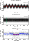 |
Fig. 2 Illustration of our transit injection and retrieval experiment. Simulations include two transits of an Earth-sized planet with an orbital period of 364 d in a 2yr light curve of an mV = 9 Sun-like star. (a) PLATO-like light curve generated with PSLS. The red line shows the trend computed with Wōtan. (b) Light curve after detrending with Wōtan. The simulated transits occur at about 91 d and 455 d (highlighted with green points), that is, near quarterly reorientations of the spacecraft. This example was deliberately chosen to illustrate that Woōtan and TLS can master non-well-behaved systems. (c) Phase-folded light curve of the transit detected with TLS. The best model fit is shown with a red line. The 21-bin walking median (ten data points symmetrically around each data point) is shown with a blue line. |
2.4 Exoplanet Occurrence Rates and Transit Probability
Petigura et al. (2013) showed that the occurrence rate of exo-planets with 2 R⊕ < Rp < 4 R⊕ and 200 d < P < 400 d around Sun-like stars is 5 (± 2.1)%. The occurrence rate of smaller planets in this period range was unconstrained. A thorough treatment of Kepler’s false positive transit events by Bryson et al. (2021) resulted in an occurrence rate of planets with radii 0.5 R⊕ < Rp < 1.5 R⊕ and inside the conservative HZs around GK stars close to ~60%, details depending on the parameterization of the HZ as a function of the stellar properties and on the reliability of exoplanet detections against systematic false positives (Bryson et al. 2020). For our purpose of estimating PLATO’s Earth-like planet yield, we assume a 37% occurrence rate in the conservative scenario and 88% in the optimistic scenario, referring to stellar population Model 1 and hab2 stars in Table 3 of Bryson et al. (2021).
PLATO’s P1 sample contains at least 15 000 and up to 20000 dwarf and subgiant bright (mV ≤ 11) stars with spectral types F5-K7. Detailed histograms for the mass, radius, effective temperature, distance, and Gaia magnitude distributions of the PLATO stellar sample have recently been published by Montalto et al. (2021), but were not available before the end of our simulations. We consider 15000 stars for our conservative scenario and 20 000 stars for our optimistic scenario. We assume that the P1 stars will be equally distributed over the NPF and SPF during the long-duration observation phase (Fig. 1), that is, we assume 7500 (or 10000) stars in each of the two fields. Hence, the (2 yr + 2 yr) strategy will contribute 15 000 stars in the conservative and 20 000 stars in the optimistic scenario. In contrast, the (3 yr + 1 yr) strategy will only contribute 7500 (or 10 000) stars to our experiment since we assume that the 1 yr field will not yield any periodic transits (only mono transits) of Earth-like planets in the HZs around Sun-like stars.
As for our neglect of finding mono transits in PLATO’s hypothetical 1 yr long-duration observation field, TLS (like BLS and similar phase-folding algorithms) is most sensitive to periodic signals. Although large-scale human inspection of thousands of light curves from the Kepler (Wang et al. 2013, 2015) and K2 missions (LaCourse & Jacobs 2018) have revealed about 200 mono transit candidates in total, the corresponding planets are all substantially larger than Earth. There have also been serendipitous mono transit discoveries with dedicated follow-up observations to confirm rare long-period transiting candidates as planets (Giles et al. 2018) and progress has been made on the methodological side with the development of new automatized search tools for mono transits (Foreman-Mackey et al. 2016; Osborn et al. 2016). But in none of these cases mono transits from Earth-sized planets have been shown to be detectable.
The geometric transit probability of an exoplanet can be approximated as Pgeo ~ Rs/a. In our case of planets at 1AU around solar-type stars we have R⊙/1 AU ~ 0.5%. We thus expect PLATO to observe (but not necessarily deliver detectable signal of) 15 000 × 37% × 0.5% ~ 28 transiting planets with 0.5 R⊕ ≤ Rp ≤ 1.5 R⊕ and orbital periods between 340 d and 760 d (within the conservative HZ) around F5-K7 dwarf stars in the conservative scenario. In the optimistic scenario, we expect observations of 20 000 × 88% × 0.5% ~ 88 such planets. The question we want to answer with our transit injection and retrieval experiment in simulated PLATO data is how many of these transits a state-of-the-art transit detection software would be able to detect.
2.5 PLATO Field of View and Star Count
For the purpose of computing PLATO’s expected planet yield, we weight the planet detection rates for different camera counts (6, 12, 18, 24) with the relative areas of the camera count coverage on the celestial plane. The combined field of view of PLATO’s 24 normal cameras is 2132 deg2. The provisional pointings of the long-duration observation fields (NPF and SPF)8 as well as the provisional pointings during the step-and-stare phase are shown in Fig. 1. Both the NPF and SPF are centered around a Galactic latitude of 30°. Though not perfectly identical, the stellar densities in the NPF and SPF are extremely similar (Fig. 8 in Nascimbeni et al. 2022). The central area of the PLATO field, which is covered by all 24 normal cameras, is 294 deg2 (13.8% of the combined field of view). The area covered by 18 cameras has a size of 171 deg2 (8.0%), by 12 cameras 796 deg2 (37.3%), and by 6 cameras 871 deg2 (40.9%) (Pertenais et al. 2021).
We also weight the planet detection rates with the relative star count as a function of apparent magnitude in these areas. We examine the Gaia Early Data Release 3 (EDR3; Gaia Collaboration 2016, 2021) and find a total of 1,247,240 stars with a G-band magnitude mG ≤ 11 in the NPF and SPF. We then broke the Gaia EDR3 star counts into the following magnitude bins, assuming similar relative star counts in the PLATO wavelength band:

The purpose of this binning was to obtain the weighting factors for the TPRs from our injection-retrieval tests that include stars of different magnitude. As for the spectral types, the distribution of stellar spectral types in the NPF and SPF was unknown at the time of our writing, and the all-sky PLATO input catalog has only been published very recently (Montalto et al. 2021). It would not have been helpful to take spectral type counts from Gaia because additional conditions are applied to the selection of the P1 sample stars in addition to magnitude cuts. Hence, we chose a Sun-like star for reference. This choice follows the procedure of using Sun-like benchmark targets in the PLATO Definition Study Report (p. 111 therein). This approximation certainly affects the expected planet yields significantly, the extent of which could be examined in future studies.
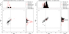 |
Fig. 3 SDE vs. S/N distribution obtained with TLS for 100 simulated 2yr light curves from 24 PLATO cameras for bright (mV = 8) Sun-like stars. (a) Light curves containing two transits of an Rp = 0.8 R⊕ planet, (b) Light curves containing two transits of an Rp = 0.9 R⊕ planet. Black lines at SDE = 9 and S/N = 7 define our nominal detection threshold. Black dots in quadrant I are true positives. Red open circles in quadrant I are false positives that are not related to quarterly jumps in the light curves. Red crossed circles in quadrant I are related to false positives caused by quarter jumps (not present in this plot but in similar plots in Appendix A). Gray dots outside of quadrant I are recoveries of the injected transit sequence but with SDE < 9 or S/N < 7 or both, that is, false negatives. Black open circles outside of quadrant I are false negatives not related to the injected signals. Black crossed circles outside of quadrant I are false negatives related to quarter jumps. The “(i)” in the legend refers to the injected signal, and “(q)” refers to quarter jumps. In the histograms, solid black bars count the number of injected signals recovered in the respective SDE or S/N bins, whereas red line bars count the number of false detections (both positives and negatives). |
2.6 Transit Injection-and-Retrieval Experiment
We create two sets of light curves with PSLS. In the pollinated set, each light curve contains a transit sequence of one planet. In the control set, no light curve contains a transit. From the pollinated sample we determine the TPR, FPR, and false negative rate (FNR). The control set is used to study the FPR and the true negative rate (TNR).
For the pollinated set, we created 2 yr and 3 yr light curves with transits for five planet radii Rp ∊ {0.8, 0.9, 1.0, 1.2, 1.4} × R⊕, four reference magnitudes тV ∊ {8, 9, 10, 11}, and assuming 24 cameras, each combination of which is represented by 100 light curves. This gives a total of 2×5×4×100 = 4000 light curves.
For Earth-sized planets only, we also simulated 2 yr and 3 yr light curves for all combinations of stellar apparent magnitudes тV ∊ {8, 9, 10, 11} and camera counts ncams ∊ {6, 12, 18, 24}, giving another 2 × 4 × 4 × 100 = 3200 light curves. For the control set, which does not contain any transits, we compute 2yr and 3 yr light curves for тV ∊ {8, 9, 10, 11} and ncams ∊ {6, 12, 18, 24}, leading again to 2 × 4 × 4 × 100 = 3200 light curves. All things combined, we generated 10400 light curves with PSLS.
For all simulated transits, we set the transit impact parameter to zero, which means that we assumed that all transits occur across the entire diameter. We also used t0 = 91 d and P = 364 d throughout our simulations; the latter choice was made to prevent a systematic effect at the Earth’s orbital period of 365.25 d that was apparent in some PSLS light curves.
We execute our computations on a (4×12)-core AMD Opteron(tm) 6174 processor (2200 MHz) on a GNU/Linux operating system with a 64-bit architecture. Computation of a 2 yr (3 yr) light curve with PSLS takes about 5 min (9 min), depending on the configuration. The detrending of a 2 yr (3 yr) light curve with Wōtan typically takes 15 min (25 min). The transit search in each 2 yr (3 yr) light curve with TLS includes periods between 50.0 d and 364.75 d (547.25 d), the upper boundary chosen to embrace the most long-period planets that exhibit at least two transits, and typically takes 4.5 h (10 h). These numbers were measured during parallel processing of typically around ten jobs, giving a total CPU time of about 270 d.
3 Results
3.1 Detection Rates
In Fig. 3 we show the SDE versus S/N distribution obtained with TLS for 100 light curves that cover 2 yr from 24 PLATO cameras. Each light curve featured one transiting planet in a 364 d orbit around an mV = 8 Sun-like star. Panel a refers to planets with a radius of 0.8 R⊕, panel b refers to Rp = 0.9 R⊕. Although TLS has the ability to search for successively weaker signals in a given light curve, we stop our search after the first detection of the strongest signal. Quadrant I, where SDE ≥ 9 and S/N ≥ 7, contains the true positives (black filled dots), that is, the retrievals of the injected transits. We define two types of false positives. Red open circles in quadrant I represent false positives not related to quarter jumps and red crossed circles illustrate false positives caused by quarter jumps. Moreover, we define three types of false negatives. One such type is a detection of the injected signal with SDE < 9 or S/N < 7 or both (gray filled dots). False negatives can also be unrelated to the injected signal and instead be caused by TLS’s detection of systematic or astrophysical variability below our nominal SDE-S/N detection threshold. If such a false negative does not refer to a detection of a quarter jump, we plot it with a black open circle. If a false negative is caused by a quarter jump outside of quadrant I, we illustrate it with a black crossed circle. The histograms along the ordinate and abscissa illustrate the SDE and S/N distributions of the injected signal recoveries (black filled bars) and false detections (red line bars), respectively.
In comparing Figs. 3a,b, we recognize a substantial shift of the SDE versus S/N distribution toward higher values, respectively. As a consequence, the TPR increases from 3% in panel a to 39% in panel b. The FPR (red symbols in quadrant I) is 4% in a and 6% in b. As a result, the detection reliability, which we define as R = TPR/(TPR + FPR), is 3/7 ~ 43% in panel a and R = 39/45 ~ 87% in panel b.
In Fig. 4 we move on to Earth-sized planets (Rp = R⊕) in one-year orbits around bright (mV = 8) Sun-like stars9. Panel a represents 100 simulated light curves obtained with 24 PLATO cameras over 2yr (similar to Fig. 3), whereas panel b shows our results for 3yr light curves. In our analysis of the 2yr light curves, each of which contains two transits, we obtain TPR = 78%, FNR = 17%, FPR = 5%, and R = 94%. For comparison, in Fig. 4b, where each light curve contained three transits, we find TPR = 100% and R = 100%.
As a major result of this study, we find that all of the injected transits of Earth-sized planets in Earth-like orbits around mV = 8 Sun-like stars are recovered when three transits are available. In fact, the increase in both SDE and S/N is significantly more pronounced when moving from two to three transits compared to increasing the planetary radius from 0.8 R⊕ to 1 R⊕. Moreover, our measurements of the detection reliability suggests that R ~ 100% for Earth-sized planets and larger.
In Fig. 5 and the following plots in this paper, we neglect any false positives detected with periods near the PLATO quarters, that is, with P = 90 (±1) d and full-integer multiples of that. Wōtan does a decent job at removing quarterly jumps (see Fig. 2), but real PLATO data will be cleaned from gaps and jumps prior to any transit search, which is why this sort of false positives will be drastically reduced in the analysis of real PLATO data. The histograms in Fig. 5 illustrate the TPRs as a function of the injected planet radius (Rp ∊ {0.8, 0.9, 1.0, 1.2, 1.4} × R⊕). For each planetary radius, we show four bars, which refer to mV ∊ {11, 10, 9, 8} from left to right, respectively. All light curves were simulated with 24 PLATO cameras. Panel a refers to 2 yr light curves with two transits, and panel b refers to 3 yr light curves with three transits.
As a general trend, and as expected, we find that the TPRs increase with increasing planetary radius in both panels a and b. In panel a, the TPRs of the 2 yr light curves are on the percent level for the smallest planets that we investigated (Rp = 0.8 R⊕), irrespective of the stellar apparent magnitude. For Rp = 0.9 R⊕, the TPRs in a increase from 9% for mV = 11 to 20% for mV = 10 and 50% for mV = 9. Interestingly, the brightest stars (mV = 8) do not yield the largest TPRs (39%), which we attribute to the associated saturation of the CCD pixels. This loss of true positives due to saturation is only present for sub-Earth-sized planets in panel a. For Earth-sized planets, the TPR is about 28% for mv = 11 and near 80% for mv ∈ {10, 9, 8}. For planets as large as or larger than 1.2 R⊕ the TPRs are near 100%.
For comparison, in panel b the TPRs of the 3 yr light curves are between about 20 and 45% for Rp = 0.8 R⊕, which represents a substantial boost from the near zero TPRs derived for these small planets in the 2 yr light curves in panel a. Moreover, the TPRs in panel b reach 80% for Rp = 0.9 R⊕ and between 91 and 100% for Rp = R⊕, details depending on the apparent stellar magnitude. For planets as large or larger than 1.2 R⊕ the TPRs are 100% for all apparent stellar magnitudes.
In Fig. 6 we focus on Earth-sized planets in one-year orbits around bright (mv = 8) Sun-like stars, showing the TPRs, the FPRs, and the FNRs. Panel a refers to 2 yr light curves with two transits, and panel b refers to 3 yr light curves with three transits. In each panel, four histograms illustrate the respective rates for 6, 12, 18, and 24 PLATO cameras (see histogram titles).
In general, the highest TPRs and lowest FNRs in Fig. 6 are obtained for the largest camera counts and lowest apparent stellar magnitudes. As a general result we find that TPRs are almost always <75% based on two transits in the 2yr light curves in panel a, even for 24 cameras and mv ∈ {8, 9, 10}. For comparison, for three transits in the 3yr light curves in panel b, TPR ≈ 100% in almost all the cases that we investigated, except for PSLS light curves simulated with 6 cameras of moderately dim stars with mv ∈ {10, 11} and for light curves from 12 cameras and mv = 11. For systems with three transits, TPRs are near 100% for mV ∈ {8, 9} and about 75% for mV = 10 even for as few as six PLATO cameras. As a consequence, an increase in the camera count is only beneficial to the TPRs of Earth-sized planets with three transits around stars with mV = 11 (and likely for even dimmer stars).
Figure 6 also demonstrates that the TPRs increase substantially for targets with low camera counts (ncams ∈ {6, 12}) when adding a third transit. This is particularly important given the fact that most of the PLATO field of view is covered with 6 cameras (40.9%) or 12 cameras (37.3%) (see Fig. 1 and Sect. 2.5). As a consequence, these areas have the greatest impact on the expected planet yields. Adding observations of a third transit is extremely beneficial to the planet yields in these regions of the PLATO field of view that are covered by 6 or 12 cameras.
Figure 7 illustrates the TNRs and FPRs obtained with TLS from PSLS light curves without any injected signal. Panel a refers to 2 yr light curves, panel b refers to 3 yr light curves. As a general result, FPRs for the 2 yr light curves in a are on the percent level at most and we do not observe any significant correlation between the FPRs and the camera count or the FPRs and the stellar apparent magnitude. For the 3 yr light curves in b, our interpretation is similar except for a dramatic increase in the FPRs to 100% for ncams = 6 and mV = 8. In this particular configuration, saturation is combined with a particularly weak transit signal and so TLS is more sensitive to the quarter jumps than to the transit.
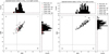 |
Fig. 4 Similar to Fig. 3 but now for Earth-sized planets around bright (mV = 8) Sun-like stars and 24 PLATO cameras. Panel a: based on two transits in 100 light curves of 2 yr length, and panel b shows the results for three transits in 100 light curves that are 3 yr long. |
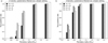 |
Fig. 5 True positive rate of our injection-and-retrieval experiment in simulated light curves from 24 PLATO cameras as a function of injected transiting planet radius. All stars are assumed to be Sun-like. A total of 100 light curves were generated, detrended, and searched for transits for each histogram bar. Detections are defined as any recovery of an injected signal within ±1 d of the injected P or T0 values and if the injected signal was detected by TLS as the strongest signal with SDE ≥ 9 and S/N ≥ 7. Results for four apparent stellar magnitudes are shown in different histogram shadings (see legend). In panel a simulated light curves have a length of 2 yr. In panel b light curves have a length of 3 yr. |
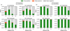 |
Fig. 6 Summary of our transit injection-and-retrieval experiment with PLATO-like light curves of Sun-like stars with an Earth-sized transiting planet in a one-year orbit. As true positives, we count TLS detections that fulfill the same criteria as those in Fig. 5. a: simulated light curves from PSLS with a duration of 2 yr and containing two transits, b: simulated light curves from PSLS with a duration of 3 yr and containing three transits. |
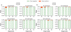 |
Fig. 7 Summary of our transit injection-and-retrieval experiment with PLATO-like light curves of Sun-like stars without any transiting planet. a: simulated light curves from PSLS with a duration of 2yr. b: simulated light curves from PSLS with a duration of 3 yr. |
3.2 Earth-like planet yield
Next, we predict PLATO’s yield of Earth-like planets in the HZ around Sun-like stars. To this purpose, we first interpolate the TPRs derived from light curves with 24 PLATO cameras to cover the entire range of planetary radii we are interested in. For the 2yr light curves, we use TPR = 0 for Rp ≤ 0.7 R⊕ and for the 3yr light curves, we use TPR = 0 for Rp ≤ 0.6 R⊕ for all magnitudes, respectively (illustrated in Fig. 5). We then use our results for the TPRs of Earth-sized planets (Fig. 6) to extrapolate the dependence of the TPRs on the camera counts across all magnitudes and planetary radii. This results in a distribution of the TPRs as a function of Rp, mV, and ncams.
As an aside, we find that under the most unfavorable conditions of ncams = 6 and mV = 11, TPRs near 100% are obtained for planets as small as 1.5R⊕ for two transits and as small as 1.3R⊕ for three transits.
We then multiply the resulting TPRs with our estimates of observable transiting Earth-like planets from Sect. 2.5. We consider both the (2 yr + 2 yr) and the (3 yr + 1 yr) strategies for PLATO’s long-duration observation phase (see Sect. 2.4). Although TLS can detect mono transits, its sensitivity is strongly diminished compared to periodic signals. Hence, we neglect mono transits in our analysis and assume that no transits will be detected during the 1 yr observation phase (see Sect. 2.4).
Our predictions of PLATO’s Earth-like planet yield are shown in Tables 1 and 2. In Table 1, planet counts are itemized as per the apparent stellar magnitude bins in which we predict them (see Sect. 2.5), whereas in Table 2 planet counts are shown as a function of the PLATO camera count. The conservative and optimistic scenarios refer to different assumptions of the star count and HZ exoplanet occurrence rate as detailed in Sect. 2.4. Although we are fully aware that only a full-integer number of exoplanets can be found, we chose to present our predictions including one decimal place given the low number counts.
The key insight to be gained from Tables 1 and 2 is that the (2 yr + 2 yr) observing strategy produces significantly higher planet yields than the (3 yr + 1 yr) observing strategy in any scenario. This interpretation is supported by the total planet yield counts in both the conservative and optimistic scenarios. The total count is 10.7 for the (2 yr + 2 yr) strategy compared to 8.0 for the (3 yr + 1 yr) strategy in the conservative scenario. In the optimistic scenario, the (2 yr + 2 yr) strategy produces a predicted yield of 33.8, whereas the (3 yr + 1 yr) strategy yields 25.4 planets. Details of the conservative versus optimistic scenarios aside, the yield of the (2 yr + 2 yr) strategy is 133% of the (3 yr + 1 yr) strategy.
In addition to these actual discoveries of small planets in the HZs around Sun-like stars, our results suggest a detection reliability near 100% for Earth-sized and larger planets (see Sect. 3.1). Hence, we do not expect a significant amount of statistical false detections, that is, false positives caused by systematic, instrumental, or statistical effects for super-Earth-sized planets. In fact, Hippke & Heller (2019) showed that an SDE threshold of 9 for TLS produces one statistical false positive in about 10 000 light curves with normally distribute noise with an amplitude of 30ppm. Consequently, the P1 sample with its 15000– 20 000 stars will yield 1–2 statistical false positives. That said, there will be about as many false detections of transiting planets smaller than Earth as there will be genuine sub-Earth-sized planets. And on top of that, there will also be false positives caused by astrophysical effects such as blended eclipsing binaries.
Estimated yield of planets with 0.5 R⊕ ≤ Rp ≤ 1.5 R⊕ in the HZs around Sun-like stars from PLATO’s P1 sample.
4 Discussion
4.1 Effects of Observing Strategy, Scenario, and Detection Thresholds
We find that the choice of the observing strategy is not as impactful as the realization of the conservative versus the optimistic scenario. The realization of the conservative or the optimistic scenario can only be affected to a limited extent, for example through the choice of the PLATO observing fields. Although neither the dilution of exoplanet transits due to stellar blending nor the occurrence of astrophysical false positives (e.g., from blended eclipsing stellar binaries) have been taken into account in our simulation, this issue has been taken care of by the PLATO consortium by optimizing the trade-off between a high number of priority targets and a low number of false-alarm detections due to crowding (Rauer et al. 2014; Nascimbeni et al. 2022). The exoplanet occurrence rate, however, which also goes into our definition of the conservative versus optimistic scenarios, is an observational property and needs to be taken as is.
In our injection-and-retrieval experiment, we used SDE = 9 and S/N = 7 as our nominal detection thresholds. The SDE versus S/N distributions in Figs. 4b and Figs. A.1b-A.3b as well as the summary plot in Fig. 5b show that these thresholds are sufficient to detect Earth-sized (and larger) planets using three transits around bright and moderately bright (mV ≤ 11) Sun-like stars with TPR > 90%. Moreover, Figs. B.1-B.4 illustrate that most false signals achieve SDE < 9 in the first transit search with TLS, although the S/N is often substantially above 10. The only type of false alarm signal with SDE > 9 that we observed in our simulations is quarter jumps, but these can be identified and dismissed. There will be other sources of false positives for PLATO, but their quantification is beyond the scope of this study. As a tribute to a rigid set of SDE and S/N thresholds, sub-Earth-sized planets are hard to be discriminated from false alarms, as becomes clear in a comparison of the SDE versus S/N distribution of the injected signals in Fig. 3 with the SDE versus S/N distribution of the control sample in Figs. B.1-B.4. The same tribute is paid for Earth-sized planets with only two transits (see Fig. 4a and Figs. A.1a-A.3a). Machine learning methods like self-organizing maps (Armstrong et al. 2017), random forest (Armstrong et al. 2018), or convolutional neural networks (Pearson et al. 2018; Osborn et al. 2020; Rao et al. 2021) might be helpful in the separation of genuine exoplanet transit signals from false alarms, but for now their advantage over smart-force search algorithms like TLS has not been conclusively demonstrated.
4.2 Planet Yields
Our focus on the strongest transit-like signal (true or false) and our omission of an iterative transit search down to the detection threshold means that we underestimate TLS’s capabilities to find shallow transits in PLATO data. In fact, TLS can automatically search for successively weaker signals (Hippke & Heller 2019) and there are several ways to interpret an iterative search in terms of true and FPRs. Though this is beyond the scope of this study iterative transit searches will certainly be an important topic for PLATO.
The TPRs for Earth-sized planets transiting mV = 8 Sunlike stars are smaller than for more moderately bright stars with mV = 9 in Figs. 5 and 6a. We attribute this effect to saturation, which results in higher-than-realistic noise levels for the brightest stars. The resulting PSLS light curves are thus not representative of real PLATO light curves. That said, these stars are also the least abundant to be observed with PLATO (see Sect. 2.5). As a consequence, we expect the effect on our expected planets yields to be minor and ≲1 in terms of number counts for all scenarios. For details of the conversion between Johnson’s V-band magnitude (mV) and PLATO’s P magnitude used in PSLS (see Marchiori et al. 2019).
A direct comparison of our predicted planet yields in the HZs around Sun-like stars with those presented in the PLATO Definition Study Report is complex due to several reasons. First, this report used analytical estimates of the expected number of planets with S/N > 10 to predict PLATO’s planet yield. For comparison, we used simulated PLATO light curves and a transit injection-and-retrieval experiment. Second, we focused on the P1 stellar sample and chose to represent its 15 000–20 000 F5–K7 stars with Sun-like stars, including astrophysical variability. Instead, the PLATO Definition Study Report included mV ≤ 11 stars from both the P1 and P5 sample, the latter of which will comprise ≥245 000 F5–K7 dwarf and subgiant stars (assuming two long-duration observation phase field pointings) with mV ≤ 13 and a cadence of 600 s in most cases. Third, the estimate of 6–280 small planets in the HZs around mV ≤ 11 stars given in the PLATO Definition Study Report included all planets smaller than 2 R⊕. By contrast, we derive exoplanet yields for 0.5R⊕ ≤ Rp ≤ 1.5R⊕. Fourth, given the large observational uncertainties at the time, the PLATO Definition Study Report necessarily included a large range of the possible occurrence rates of small planets in the HZ around Sun-like stars of between 2 and 100%. For comparison, our planet yield predictions are based on updated occurrence rates estimates (Bryson et al. 2021), which define our conservative scenario with 37% and our optimistic scenario with 88%.
Our yield estimates for planets with 0.5 R⊕ ≤ Rp ≤ 1.5 R⊕ range between 11 in the conservative scenario of the (2yr + 2 yr) observing strategy (or 8 for the 3 yr + 1 yr observing strategy) and 34 in the optimistic scenario of the (2 yr + 2 yr) observing strategy (or 25 for the 3 yr + 1 yr observing strategy) (see Tables 1 and 2). With all the caveats of a direct comparison in mind, our range of the predicted yield of small planets in the HZ is much tighter than the previous estimates from the PLATO Definition Study Report and tends to fall in the lower regime of the previous planet yield estimates.
4.3 Methodological Limitations and Improvements
Our results demonstrate that the Wōtan detrending software efficiently removes stellar and systematic variability while preserving transit signatures. That said, in some cases we find that Woōtan does not effectively remove quarter jumps from PSLS light curves. Wōotan has been designed to detrend jumps by stitching the data prior and after gaps in the light curve, a functionality that can be fine-tuned using the break_tolerance parameter. Real PLATO data will indeed have gaps of at least several hours required for satellite repositioning, which can be stitched with Woōtan. But PSLS does not include temporal gaps at quarter jumps for now. This results in occasional false positive detections with TLS at these quarter jumps, in particular for stars with mV ≥ 10 (see Figs. A.3, B.3, and B.4).
In the final data products of the actual PLATO mission, quarter jumps will be subjected to a dedicated light curve stitching. As a consequence, this type of false positives will not, or very rarely, be an issue. As explained in Sect. 3.1, this is why we neglect quarterly false positives in our summary plots (Figs. 5-7). Nevertheless, since we did not attempt to sort out false positives detected with TLS at quarterly jumps and then rerun TLS, we can expect that the TPRs derived with TLS in such an iterative manner could actually be higher than shown in Figs. 5 and 6. As a consequence, the application of TLS on a set of light curves that were properly corrected for quarter jumps can be expected to produce slightly higher planet yields than in Tables 1 and 2.
PSLS (v1.3) includes long-term drift correction. It corrects for the drift in the CCD positions of the stars due to relativistic velocity aberration and satellite motion. It does not currently take into account, however, any detrending of the light curves from jitter, CCD positional changes from thermal trends induced by spacecraft rotation every three months, regular thermal perturbations caused by the daily data transfer, momentum wheel desaturation, residual outliers not detected by the outlier detection algorithms, or the stitching of parts of the light curves between mask updates – the last of which is irrelevant for P1 sample stars since their photometry will be extracted using a fitting of the point spread function. Although Wotan can be expected to remove most of these trends in a reasonable manner while preserving transit signatures, the actual data products of the PLATO mission will be subjected to a detailed detrending of systematic effects. In terms of detrending of systematic effects (but not necessarily of astrophysical variability), the real PLATO data will therefore have a somewhat better quality for transit searches than the PSLS light curves that we used.
On the down side, our simulations assume near-continuous uptime and uninterrupted functionality of the PLATO satellite. This might be overly optimistic as demonstrated by the Kepler mission, which achieved an average of ~90% time on target. Unplanned downtimes of PLATO might outbalance the benefits of improved systematic detrending so that our values in Tables 1 and 2 would remain almost unaffected.
We restricted our study to stars with solar-like activity, while the actual stars to be observed in the P1 sample will naturally exhibit a range of activity patterns. An analysis of the first six months of continuous observations of moderately bright stars (Kepler magnitudes 10.5 ≤ Kp ≤ 11.5) from the Kepler primary mission showed that solar-type stars are intrinsically more active than previously thought (Gilliland et al. 2011), a result later confirmed with the final four years of Kepler observations (Gilliland et al. 2015). Our assumptions of solar-like activity might thus be overly optimistic. This might have a negative effect on the planet yields that we estimate since transit signatures of small planets are harder to find around photometrically more active stars. Simulations of PLATO-like light curves with more realistic intrinsic stellar variability is, in principle, possible with PSLS. For now, PSLS requires a user-defined parameterization of stellar activity but future versions are planned to implement empirical descriptions of the magnetic activity to suit PLATO solar-like oscillators (Samadi et al. 2019). Moreover, rotational modulation caused by spots on the surface of the star are not yet implemented in PSLS.
We did not simulate a representative population of 15000 to 20 000 F5–K7 stars with mV ≤ 11 as will be observed in PLATO’s P1 stellar sample. Instead, we assumed a solar-type star with solar radius and mass, investigated four apparent stellar magnitudes mV ∈ {8, 9, 10, 11} for reference simulations with PSLS, and weighted the abundance of stars in one-magnitude bins around these reference magnitudes (Sect. 2.5). There are at least three caveats with this assumption. First, the apparent magnitude distribution of the P1 sample will likely differ from that of field stars, with a drop between mV = 10 and mV = 11 since the outer, low-camera-count regions of PLATO’s field of view are not able to meet the noise limit requirement of 50 ppm per hour integration (V. Nascimbeni, priv. comm.). Second, Sun-like stars will likely be underrepresented compared to more early-type stars in the P1 sample. The median stellar radius in the P1 sample will likely be closer to 1.3 R⊙ (Montalto et al. 2021), roughly corresponding to spectral type F0 on the main sequence. The HZ will be farther away from the star than in our simulations and the orbital period will be larger than 1 yr. And third, the P1 sample is not supposed to be evenly distributed over PLATO’s NPF and SPF due to the noise limit requirement. Instead, the P1 sample stars will be concentrated in the inner part of the NPF and SPF, where they are covered by 18 or 24 telescopes. In summary, we expect that (1) the apparent magnitude distribution of the P1 sample stars will be skewed more toward brighter stars than based on our Gaia counts of fields stars (Sect. 2.5), (2) transits of Earth-sized planets in the HZs around P1 sample stars will typically be shallower and have longer orbital periods than the transits around nominal Sun-like stars in our simulations, and (3) the P1 sample stars will preferentially be observed with 18 or 24 cameras. Since points (1) and (3) have an opposite effect on the planet yield to point (2) it is impossible, based on the currently available data, to specify the resulting effect on the actual planet yield presented in this paper.
In all our transit simulations, we assumed a transit impact parameter of zero, that is, that the planet crosses the star along the apparent stellar diameter. In reality, however, the average transit impact parameter for a large sample of transiting planets is π/4 ~ 79% of that value (Jenkins et al. 2002). As a result, we overestimate the average transit duration (and therefore the resulting S/N) around a large sample of Sun-like stars systematically. That said, this effect is mitigated by the longer transit durations expected for HZ planets in the P1 sample, as explained above.
5 Conclusions
We have developed a procedure to estimate the yield of Earthlike planets in the HZs around Sun-like stars from the PLATO mission. In brief, we simulated PLATO-like light curves, some of which included transits, with the PSLS software, performed a detrending from systematic and astrophysical variability with the Wotan software, and then searched for the injected signals with the TLS search algorithm. We combined our measurements of the TPRs with the expected number of stars in PLATO’s P1 stellar sample of bright (mV ≤ 11) stars and with modern estimates for the occurrence rate of Earth-sized planets in the HZs around Sun-like stars to predict PLATO’s exoplanet yield. We investigated the (2 yr + 2 yr) and the (3 yr + 1 yr) observation strategies for PLATO’s long-duration observation phase fields.
We find that under the same simulation conditions the (2 yr + 2 yr) observing strategy results in significantly enhanced planet yields compared to the (3 yr + 1 yr) strategy. Details of the exact numbers for both strategies depend on the actual number of stars that will be observed in the P1 sample and on the occurrence rate of small planets in the HZs around Sun-like stars.
Under the assumption of a Sun-like star with low stellar activity, we find that PLATO can detect planets with radii ≥ 1.2 R⊕ with TPR ~ 100% in the P1 sample (mV ≤ 11) if two transits can be observed synchronously by 24 PLATO cameras. When a third transit is added under otherwise unchanged conditions, TPR ~ 100% is achieved for planet as small as Earth. True positive rates of a few percent for planets as small as 0.8 R⊕ in one-year orbits around bright Sun-like stars from the P1 sample suggest that this is the minimum planet size that can be detected, in some rare and photometrically optimal cases, if two transits are observed. If three transits are available, planets as small as 0.7 R⊕ may be detectable in rare cases.
Assuming the most unfavorable conditions in our setup with only six PLATO cameras and transits in front of the dimmest Sun-like stars in PLATO’s P1 sample (mV = 11), TPRs near 100% are nevertheless achieved for planets as small as 1.5 R⊕ for two transits and as small as 1.3 R⊕ for three transits around solar-type stars. Again, these estimates all assume low, Sun-like photometric variability.
Using the Sun as a proxy, we predict the detection of between 8 and 34 Earth-like planets in the HZs around F5–K7 main-sequence stars with 0.5 R⊕ ≤ Rp ≤ 1.5R⊕. These estimates should be considered an upper limit for several reasons. First, given that PLATO’s P1 sample stars will typically be larger than the Sun-like benchmark stars in our simulations (Montalto et al. 2021), the resulting transits of Earth-like planets in the HZ will be shallower and less frequent than we simulated. Second, astro-physical false positives, which we neglected, and as yet unknown systematic effects of the PLATO mission might increase the FPR and complicate the identification of genuine transits, in particular given the low number of transits expected for Earthlike planets in the HZs around Sun-like stars. Third, and maybe most importantly, all our estimates are based on simulations of photometrically quiet Sun-like stars, whereas in reality most F5– K7 main-sequence stars are photometrically more variable. On the other hand, a more sophisticated correction of systematic effects and astrophysical variability, more elaborate vetting than a mere SDE-S/N cut, a bias of the P1 stellar sample toward bright stars covered with 18 or 24 cameras, and serendipitous discoveries in PLATO’s P2–P5 stellar samples could lead to additional discoveries that are not considered in our estimates.
Our results suggest that PLATO can achieve its science objective of finding Earth-like planets in the HZs around Sunlike stars. The prediction of the discovery of 8–34 such worlds means a substantial step forward from the previously available estimates that ranged between 6 and 280. Nevertheless, our new estimates worryingly remind us of the initial predictions for the number of Earth-like planets to be discovered with NASA’s Kepler mission, which fluctuated around 50 over the years (Borucki et al. 1996; Borucki 2016). These estimates for Kepler relied on the Sun as a proxy for stellar variability, which turned out to be an overly optimistic approach. Hence, our results require follow-up studies of PLATO’s expected planet yield with more realistic stellar variability. If shallow transit detection can be achieved in the presence of significant stellar variability, then our results suggest that PLATO’s detections will mean a major contribution to this as yet poorly sampled regime of the exoplanet parameter space with Earth-sized planets in the HZs around solar-type stars.
Acknowledgements
The authors thank Valerio Nascimbeni, Michael Hippke, Heike Rauer, Juan Cabrera, and Carlos del Burgo for helpful comments on the manuscript. They are also thankful to an anonymous referee for a thorough report. R.H. acknowledges support from the German Aerospace Agency (Deutsches Zentrum für Luft- und Raumfahrt) under PLATO Data Center grant 50OO1501. R.S. acknowledges financial support by the Centre National D’Etudes Spatiales (CNES) for the development of psls. This work presents results from the European Space Agency (ESA) space mission PLATO. The PLATO payload, the PLATO Ground Segment and PLATO data processing are joint developments of ESA and the PLATO Mission Consortium (PMC). Funding for the PMC is provided at national levels, in particular by countries participating in the PLATO Multilateral Agreement (Austria, Belgium, Czech Republic, Denmark, France, Germany, Italy, Netherlands, Portugal, Spain, Sweden, Switzerland, Norway, and UK) and institutions from Brazil. Members of the PLATO Consortium can be found at https://platomission.com. The ESA PLATO mission website is https://www.cosmos.esa.int/plato. We thank the teams working for PLATO for all their work. This work has made use of data from the European Space Agency (ESA) mission Gaia (https://www.cosmos.esa.int/gaia), processed by the Gaia Data Processing and Analysis Consortium (DPAC, https://www.cosmos.esa.int/web/gaia/dpac/consortium). Funding for the DPAC has been provided by national institutions, in particular the institutions participating in the Gaia Multilateral Agreement.
Appendix A SDE Versus S/N for Earth-Sized Planets and 24 PLATO Cameras
As an extension of Fig. 4 we provide the SDE versus S/N distribution of transiting Earth-like planets around more moderately bright Sun-like stars from the P1 sample. All PSLS light curves analyzed for these plots assume observations observed with 24 cameras. Figure A.1 refers to mv = 9, Fig. A.2 refers to mv = 10, and Fig. A.3 refers to mv = 11 Sun-like stars.
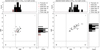 |
Fig. A.1 SDE vs. S/N for 100 simulated light curves of an mv = 9 Sun-like star with a 1 R⊕ transiting planet observed with 24 PLATO cameras. Left: Each simulated 2 yr light curve contained two transits. Right: Each simulated 3 yr light curve contained three transits. |
Appendix B SDE Versus S/N for 24 PLATO Cameras without Injections
In addition to the SDE versus SDE diagrams for our injection-and-retrieval tests, we also generated similar plots for the control sample of light curves, which did not contain any injected transits. These simulations are key to determining the TNRs and FPRs shown in Fig. 7. The following plots are all based on simulated PSLS observations with 24 PLATO cameras. Figure B.1 refers to mv = 8, Fig. B.2 refers to mv = 9, Fig. B.3 refers to mv = 10, and Fig. B.4 refers to mv = 11.
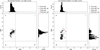 |
Fig. B.1 SDE vs. S/N for 100 simulated light curves of an mv = 8 Sun-like star with no injected transiting planet observed with 24 PLATO cameras. Left: 2 yr light curves. Right: 3 yr light curves. |
Appendix C Transits in the Presence of Stellar Activity
Throughout our study we have assumed a Sun-like star with solar activity levels. This assumption had also been made prior to the Kepler mission and unfortunately the analysis of stellar activity levels of the Kepler stars has shown that this assumption was too optimistic. As it turned out, the Sun is a relatively quiet star, from the perspective of photometric variability (Gilliland et al. 2011, 2015). The underestimation of stellar variability prior to the Kepler mission is now seen as a main reason for why the mission could not achieve the detection of an Earth-sized planet with three transits, that is, in a one-year orbit around a solar-type star. PLATO will naturally face the same challenges. Although a detailed investigation of the effects of stellar variability on transit detectability is beyond the scope of this manuscript, we have executed a limited qualitative study.
In discussing stellar activity in the context of exoplanet transits, various metrics are in use throughout the community. For example, García et al. (2014) measure 〈Sph,k〉, the mean standard deviation in a running window with a width corresponding to k times the rotation period of a given star. As such, 〈Sph,k〉 correlates with the amplitude of the stellar activity component used in the simulations with PSLS (σA) (Douaglin 2018), which is given in Eq. (37) in Samadi et al. (2019). Beyond stellar activity, 〈Sph,k〉 takes into account any kind of instrumental or systematic error in the light curves and, hence, has the tendency to exceed the stellar activity component. In our analysis we take a similar approach and measure the combined noise level as the standard deviation in a sliding window with a width of 1 hr (σ1 hr), which is the reference timescale for the computation of the noise-to-signal budgets in the PLATO mission (Rauer et al. 2014). As an aside, another alternative metric was used by the Kepler mission, which applied the “combined differential photometric precision” (Jenkins et al. 2010).
To examine transits in light curves with different stellar activity levels, we simulated three stars of solar radius with increasing stellar activity levels and on different characteristic timescales: (1) σA = 40 ppm and τA = 0.8 d; (2) σA = 166 ppm and τA = 0.5 d; and (3) σA = 500ppm and τA = 0.3 d. The choice of the timescale is motivated by findings of Hulot et al. (2011), who measured the characteristic timescales for the evolution of stellar activity. As an aside, τA used in PSLS corresponds to the timescales of Hulot et al. (2011) divided by 2π. As for the activity levels, we refer to García et al. (2014), who determined for the Sun that 〈Sph,k〉, referred to as its photometric magnetic activity level, ranges between 89 ppm and 259 ppm with a reference value of 166 ppm.
For each star, we generated 40 light curves with two transits of an Earth-like planet and an equal amount of light curves without transits. In each light curve we measured the sliding standard deviation in a 1 hr window as a proxy for the combined activity on that timescale (σ1 hr). All simulations assumed an apparent stellar magnitude of mv = 9 and coverage by 24 PLATO cameras. Our measurements of σ1 hr for the three benchmark stars are given in Table C.1. In Figs. C.1-Figs. C.3 we show some examples of the resulting light curves, each of which includes a transit of an Earth-like planet. In our preliminary analysis, we found that the transit detectability with TLS upon detrending with Wōtan depends sensitively on σA but weakly on τA. As we quantified in a limited injection-recovery test, shallow transits of Earth-sized planets are securely recovered around the quiet benchmark star (Fig. C.1) but a large fraction of them gets lost in the stellar activity around even the moderately active benchmark star (Fig. C.2) and they become entirely undetectable around the more active stars (Fig. C.3). These findings illustrate that our estimates of PLATO planet yield, which we derived using a photometrically quiet star, must be seen as upper limits.
Stellar activity measurements from simulated PSLS light curves.
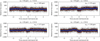 |
Fig. C.1 Four example light curves generated with PSLS with a transit of an Earth-like planet around a solar-sized star with weak photometric activity (σA = 40 ppm, τA = 0:8 d). The light curves assumed synchronous observations with 24 PLATO cameras and mV = 9. The duration of the transit is indicated with two vertical black bars spanning a window of 12 hr around the mid-transit time. |
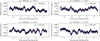 |
Fig. C.3 Same as Fig. C.1 but for an active star (σA = 500 ppm, τA = 0.3 d). Note the vastly different range along the ordinate compared to Figs. C.1 and C.2. |
References
- Anderson, E. R., Duvall, Thomas L.J., & Jefferies, S. M. 1990, ApJ, 364, 699 [NASA ADS] [CrossRef] [Google Scholar]
- Armstrong, D. J., Pollacco, D., & Santerne, A. 2017, MNRAS, 465, 2634 [NASA ADS] [CrossRef] [Google Scholar]
- Armstrong, D. J., Günther, M. N., McCormac, J., et al. 2018, MNRAS, 478, 4225 [NASA ADS] [CrossRef] [Google Scholar]
- Auvergne, M., Bodin, P., Boisnard, L., et al. 2009, A&A, 506, 411 [NASA ADS] [CrossRef] [EDP Sciences] [Google Scholar]
- Berthomieu, G., Toutain, T., Gonczi, G., et al. 2001, ESA SP, 464, 411 [Google Scholar]
- Borucki, W. J. 2016, Rep. Prog. Phys., 79, 036901 [Google Scholar]
- Borucki, W. J., Dunham, E. W., Koch, D. G., et al. 1996, Ap&SS, 241, 111 [NASA ADS] [CrossRef] [Google Scholar]
- Borucki, W. J., Koch, D., Basri, G., et al. 2010, Science, 327, 977 [Google Scholar]
- Bryson, S., Coughlin, J., Batalha, N. M., et al. 2020, AJ, 159, 279 [NASA ADS] [CrossRef] [Google Scholar]
- Bryson, S., Kunimoto, M., Kopparapu, R. K., et al. 2021, AJ, 161, 36 [NASA ADS] [CrossRef] [Google Scholar]
- Charbonneau, D., Brown, T. M., Latham, D. W., & Mayor, M. 2000, ApJ, 529, L45 [Google Scholar]
- Christensen-Dalsgaard, J. 2008, Astrophys. Space Sci., 316, 113 [NASA ADS] [CrossRef] [Google Scholar]
- Davies, G. R., Chaplin, W. J., Farr, W. M., et al. 2015, MNRAS, 446, 2959 [CrossRef] [Google Scholar]
- Deleuil, M., Aigrain, S., Moutou, C., et al. 2018, A&A, 619, A97 [NASA ADS] [CrossRef] [EDP Sciences] [Google Scholar]
- Douaglin, Q. 2018, Master’s thesis, Observatoire de Paris, France [Google Scholar]
- Feliz, D. L., Plavchan, P., Bianco, S. N., et al. 2021, AJ, 161, 247 [Google Scholar]
- Foreman-Mackey, D., Morton, T. D., Hogg, D. W., Agol, E., & Schölkopf, B. 2016, AJ, 152, 206 [NASA ADS] [CrossRef] [Google Scholar]
- Fressin, F., Torres, G., Charbonneau, D., et al. 2013, ApJ, 766, 81 [NASA ADS] [CrossRef] [Google Scholar]
- Gaia Collaboration (Prusti, T., et al.) 2016, A&A, 595, A1 [NASA ADS] [CrossRef] [EDP Sciences] [Google Scholar]
- Gaia Collaboration (Brown, A. G. A., et al.) 2021, A&A, 649, A1 [NASA ADS] [CrossRef] [EDP Sciences] [Google Scholar]
- García, R. A., Ceillier, T., Salabert, D., et al. 2014, A&A, 572, A34 [NASA ADS] [CrossRef] [EDP Sciences] [Google Scholar]
- Giles, H. A. C., Osborn, H. P., Blanco-Cuaresma, S., et al. 2018, A&A, 615, L13 [NASA ADS] [CrossRef] [EDP Sciences] [Google Scholar]
- Gilliland, R. L., Chaplin, W. J., Dunham, E. W., et al. 2011, ApJS, 197, 6 [NASA ADS] [CrossRef] [Google Scholar]
- Gilliland, R. L., Chaplin, W. J., Jenkins, J. M., Ramsey, L. W., & Smith, J. C. 2015, AJ, 150, 133 [Google Scholar]
- Heller, R., & Kiss, L. 2019, ArXiv e-prints [arXiv:1911.12114] [Google Scholar]
- Heller, R., Hippke, M., & Rodenbeck, K. 2019a, A&A, 627, A66 [NASA ADS] [CrossRef] [EDP Sciences] [Google Scholar]
- Heller, R., Rodenbeck, K., & Hippke, M. 2019b, A&A, 625, A31 [NASA ADS] [CrossRef] [EDP Sciences] [Google Scholar]
- Heller, R., Hippke, M., Freudenthal, J., et al. 2020, A&A, 638, A10 [NASA ADS] [CrossRef] [EDP Sciences] [Google Scholar]
- Hippke, M., & Heller, R. 2019, A&A, 623, A39 [NASA ADS] [CrossRef] [EDP Sciences] [Google Scholar]
- Hippke, M., David, T. J., Mulders, G. D., & Heller, R. 2019, AJ, 158, 143 [Google Scholar]
- Howell, S. B., Sobeck, C., Haas, M., et al. 2014, PASP, 126, 398 [Google Scholar]
- Hsu, D. C., Ford, E. B., Ragozzine, D., & Ashby, K. 2019, AJ, 158, 109 [NASA ADS] [CrossRef] [Google Scholar]
- Hulot, J. C., Baudin, F., Samadi, R., & Goupil, M. J. 2011, ArXiv e-prints [arXiv:1104.2185] [Google Scholar]
- Janesick, J. 2001, Scientific Charge-coupled Devices, Press Monograph Series (USA: Society of Photo Optical) [CrossRef] [Google Scholar]
- Jenkins, J. M., Caldwell, D. A., & Borucki, W. J. 2002, ApJ, 564, 495 [NASA ADS] [CrossRef] [Google Scholar]
- Jenkins, J. M., Chandrasekaran, H., McCauliff, S. D., et al. 2010, SPIE Conf. Ser., 7740, 77400D [Google Scholar]
- Jenkins, J. M., Twicken, J. D., Batalha, N. M., et al. 2015, AJ, 150, 56 [NASA ADS] [CrossRef] [Google Scholar]
- Kasting, J. F., Whitmire, D. P., & Reynolds, R. T. 1993, Icarus, 101, 108 [Google Scholar]
- Kopparapu, R. K., Ramirez, R. M., SchottelKotte, J., et al. 2014, ApJ, 787, L29 [Google Scholar]
- Kovács, G., Zucker, S., & Mazeh, T. 2002, A&A, 391, 369 [Google Scholar]
- Kunimoto, M., & Matthews, J. M. 2020, AJ, 159, 248 [NASA ADS] [CrossRef] [Google Scholar]
- LaCourse, D. M., & Jacobs, T. L. 2018, Res. Notes Am. Astron. Soc., 2, 28 [Google Scholar]
- Lauer, T. R. 1999, PASP, 111, 1434 [NASA ADS] [CrossRef] [Google Scholar]
- Mandel, K., & Agol, E. 2002, ApJ, 580, L171 [Google Scholar]
- Marchiori, V., Samadi, R., Fialho, F., et al. 2019, A&A, 627, A71 [NASA ADS] [CrossRef] [EDP Sciences] [Google Scholar]
- Marcos-Arenal, P., Zima, W., De Ridder, J., et al. 2014, A&A, 566, A92 [NASA ADS] [CrossRef] [EDP Sciences] [Google Scholar]
- Montalto, M., Piotto, G., Marrese, P. M., et al. 2021, A&A, 653, A98 [NASA ADS] [CrossRef] [EDP Sciences] [Google Scholar]
- Morris, B. M., Bobra, M. G., Agol, E., Lee, Y. J., & Hawley, S. L. 2020, MNRAS, 493, 5489 [NASA ADS] [CrossRef] [Google Scholar]
- Mulders, G. D., Mordasini, C., Pascucci, I., et al. 2019, ApJ, 887, 157 [NASA ADS] [CrossRef] [Google Scholar]
- Mullally, F., Thompson, S. E., Coughlin, J. L., Burke, C. J., & Rowe, J. F. 2018, AJ, 155, 210 [NASA ADS] [CrossRef] [Google Scholar]
- Nascimbeni, V., Piotto, G., Börner, A., et al. 2022, A&A, 658, A31 [NASA ADS] [CrossRef] [EDP Sciences] [Google Scholar]
- Osborn, H. P., Armstrong, D. J., Brown, D. J. A., et al. 2016, MNRAS, 457, 2273 [NASA ADS] [CrossRef] [Google Scholar]
- Osborn, H. P., Ansdell, M., Ioannou, Y., et al. 2020, A&A, 633, A53 [NASA ADS] [CrossRef] [EDP Sciences] [Google Scholar]
- Pearson, K. A., Palafox, L., & Griffith, C. A. 2018, MNRAS, 474, 478 [NASA ADS] [CrossRef] [Google Scholar]
- Pertenais, M., Cabrera, J., Paproth, C., et al. 2021, SPIE, 11852, 2061 [Google Scholar]
- Petigura, E. A., Howard, A. W., & Marcy, G. W. 2013, Proc. Natl. Acad. Sci., 110, 19273 [Google Scholar]
- Pont, F., Zucker, S., & Queloz, D. 2006, MNRAS, 373, 231 [NASA ADS] [CrossRef] [Google Scholar]
- Rao, S., Mahabal, A., Rao, N., & Raghavendra, C. 2021, MNRAS, 502, 2845 [NASA ADS] [CrossRef] [Google Scholar]
- Rauer, H., Catala, C., Aerts, C., et al. 2014, Exp. Astron., 38, 249 [Google Scholar]
- Ricker, G. R., Winn, J. N., Vanderspek, R., et al. 2015, J. Astron. Teles. Instrum. Syst., 1, 014003 [Google Scholar]
- Samadi, R., Deru, A., Reese, D., et al. 2019, A&A, 624, A117 [NASA ADS] [CrossRef] [EDP Sciences] [Google Scholar]
- Short, A., Crowley, C., de Bruijne, J. H. J., & Prod’homme, T. 2013, MNRAS, 430, 3078 [Google Scholar]
- Thompson, S. E., Coughlin, J. L., Hoffman, K., et al. 2018, ApJS, 235, 38 [NASA ADS] [CrossRef] [Google Scholar]
- Trifonov, T., Caballero, J. A., Morales, J. C., et al. 2021, Science, 371, 1038 [Google Scholar]
- Van Cleve, J. E., & Caldwell, D. A. 2016, Kepler Instrument Handbook, Tech. rep., http://archive.stsci.edu/kepler/manuals/KSCI-19033-002.pdf [Google Scholar]
- Van Grootel, V., Pozuelos, F. J., Thuillier, A., et al. 2021, A&A, 650, A205 [NASA ADS] [CrossRef] [EDP Sciences] [Google Scholar]
- Wang, J., Fischer, D. A., Barclay, T., et al. 2013, ApJ, 776, 10 [NASA ADS] [CrossRef] [Google Scholar]
- Wang, J., Fischer, D. A., Barclay, T., et al. 2015, ApJ, 815, 127 [NASA ADS] [CrossRef] [Google Scholar]
NASA Exoplanet Archive, https://exoplanetarchive.ipac.caltech.edu, as of 20 June 2022.
PLATO Definition Study Report, https://sci.esa.int/s/8rPyPew
The 24 “normal” cameras will observe stars with apparent visual magnitudes mV ≳ 8 in white light with a cadence of 25 s. Two additional “fast” cameras will observe very bright stars with 4 ≲ mV ≲ 8 in two different color filters (one in a blue filter, the other in a red filter) with a cadence of 2.5 s. The fast cameras will be used for color refinements of astrophysical processes and fine guidance.
The provisional NPF has been designed to overlap with the field of the Kepler primary mission. Though not a primary focus of PLATO, this overlap might allow for the validation of a significant number of Kepler exoplanet candidates and could help to secure exoplanet ephemeris.
The SDE vs. S/N distributions obtained for injection and retrieval experiments with Rp = R⊕ for both 2yr and 3yr light curves of Sun-like stars with mV ∊ {9, 10, 11}, all of which assumed 24 cameras, are available in Appendix A.
All Tables
Estimated yield of planets with 0.5 R⊕ ≤ Rp ≤ 1.5 R⊕ in the HZs around Sun-like stars from PLATO’s P1 sample.
All Figures
|
Fig. 1 Provisional pointing of PLATO’s northern (NPF) and southern (SPF) long-duration phase fields in an all-sky Aitoff projection using Galactic coordinates (an updated version is available in Nascimbeni et al. 2022). The centers of the NPF and SPF are covered by 24 cameras (light blue). Increasingly darker blue tones refer to a coverage by 18, 12, and 6 cameras, respectively. Provisional step-and-stare field pointings (STEP01 – STEP10) use dark blue tones for an overlap of 24 cameras and lighter blue tones for 18, 12, and 6 cameras, respectively. The fields of CoRoT (pink), Kepler (red), K2 (green), and the TESS continuous viewing zone (yellow) are also shown. |
| In the text | |
|
Fig. 2 Illustration of our transit injection and retrieval experiment. Simulations include two transits of an Earth-sized planet with an orbital period of 364 d in a 2yr light curve of an mV = 9 Sun-like star. (a) PLATO-like light curve generated with PSLS. The red line shows the trend computed with Wōtan. (b) Light curve after detrending with Wōtan. The simulated transits occur at about 91 d and 455 d (highlighted with green points), that is, near quarterly reorientations of the spacecraft. This example was deliberately chosen to illustrate that Woōtan and TLS can master non-well-behaved systems. (c) Phase-folded light curve of the transit detected with TLS. The best model fit is shown with a red line. The 21-bin walking median (ten data points symmetrically around each data point) is shown with a blue line. |
| In the text | |
|
Fig. 3 SDE vs. S/N distribution obtained with TLS for 100 simulated 2yr light curves from 24 PLATO cameras for bright (mV = 8) Sun-like stars. (a) Light curves containing two transits of an Rp = 0.8 R⊕ planet, (b) Light curves containing two transits of an Rp = 0.9 R⊕ planet. Black lines at SDE = 9 and S/N = 7 define our nominal detection threshold. Black dots in quadrant I are true positives. Red open circles in quadrant I are false positives that are not related to quarterly jumps in the light curves. Red crossed circles in quadrant I are related to false positives caused by quarter jumps (not present in this plot but in similar plots in Appendix A). Gray dots outside of quadrant I are recoveries of the injected transit sequence but with SDE < 9 or S/N < 7 or both, that is, false negatives. Black open circles outside of quadrant I are false negatives not related to the injected signals. Black crossed circles outside of quadrant I are false negatives related to quarter jumps. The “(i)” in the legend refers to the injected signal, and “(q)” refers to quarter jumps. In the histograms, solid black bars count the number of injected signals recovered in the respective SDE or S/N bins, whereas red line bars count the number of false detections (both positives and negatives). |
| In the text | |
|
Fig. 4 Similar to Fig. 3 but now for Earth-sized planets around bright (mV = 8) Sun-like stars and 24 PLATO cameras. Panel a: based on two transits in 100 light curves of 2 yr length, and panel b shows the results for three transits in 100 light curves that are 3 yr long. |
| In the text | |
|
Fig. 5 True positive rate of our injection-and-retrieval experiment in simulated light curves from 24 PLATO cameras as a function of injected transiting planet radius. All stars are assumed to be Sun-like. A total of 100 light curves were generated, detrended, and searched for transits for each histogram bar. Detections are defined as any recovery of an injected signal within ±1 d of the injected P or T0 values and if the injected signal was detected by TLS as the strongest signal with SDE ≥ 9 and S/N ≥ 7. Results for four apparent stellar magnitudes are shown in different histogram shadings (see legend). In panel a simulated light curves have a length of 2 yr. In panel b light curves have a length of 3 yr. |
| In the text | |
|
Fig. 6 Summary of our transit injection-and-retrieval experiment with PLATO-like light curves of Sun-like stars with an Earth-sized transiting planet in a one-year orbit. As true positives, we count TLS detections that fulfill the same criteria as those in Fig. 5. a: simulated light curves from PSLS with a duration of 2 yr and containing two transits, b: simulated light curves from PSLS with a duration of 3 yr and containing three transits. |
| In the text | |
|
Fig. 7 Summary of our transit injection-and-retrieval experiment with PLATO-like light curves of Sun-like stars without any transiting planet. a: simulated light curves from PSLS with a duration of 2yr. b: simulated light curves from PSLS with a duration of 3 yr. |
| In the text | |
|
Fig. A.1 SDE vs. S/N for 100 simulated light curves of an mv = 9 Sun-like star with a 1 R⊕ transiting planet observed with 24 PLATO cameras. Left: Each simulated 2 yr light curve contained two transits. Right: Each simulated 3 yr light curve contained three transits. |
| In the text | |
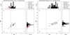 |
Fig. A.2 Similar to Fig. A.1 but for an mv = 10 Sun-like star. |
| In the text | |
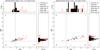 |
Fig. A.3 Similar to Fig. A.1 but for an mv = 11 Sun-like star. |
| In the text | |
|
Fig. B.1 SDE vs. S/N for 100 simulated light curves of an mv = 8 Sun-like star with no injected transiting planet observed with 24 PLATO cameras. Left: 2 yr light curves. Right: 3 yr light curves. |
| In the text | |
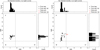 |
Fig. B.2 Similar to Fig. B.1 but for an mv = 9 Sun-like star. |
| In the text | |
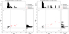 |
Fig. B.3 Similar to Fig. B.1 but for an mv = 10 Sun-like star. |
| In the text | |
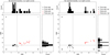 |
Fig. B.4 Similar to Fig. B.1 but for an mv = 11 Sun-like star. |
| In the text | |
|
Fig. C.1 Four example light curves generated with PSLS with a transit of an Earth-like planet around a solar-sized star with weak photometric activity (σA = 40 ppm, τA = 0:8 d). The light curves assumed synchronous observations with 24 PLATO cameras and mV = 9. The duration of the transit is indicated with two vertical black bars spanning a window of 12 hr around the mid-transit time. |
| In the text | |
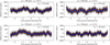 |
Fig. C.2 Same as Fig. C.1 but for a moderately active star (σA = 166 ppm, τA = 0.5 d). |
| In the text | |
|
Fig. C.3 Same as Fig. C.1 but for an active star (σA = 500 ppm, τA = 0.3 d). Note the vastly different range along the ordinate compared to Figs. C.1 and C.2. |
| In the text | |
Current usage metrics show cumulative count of Article Views (full-text article views including HTML views, PDF and ePub downloads, according to the available data) and Abstracts Views on Vision4Press platform.
Data correspond to usage on the plateform after 2015. The current usage metrics is available 48-96 hours after online publication and is updated daily on week days.
Initial download of the metrics may take a while.