| Issue |
A&A
Volume 694, February 2025
|
|
|---|---|---|
| Article Number | A267 | |
| Number of page(s) | 17 | |
| Section | Cosmology (including clusters of galaxies) | |
| DOI | https://doi.org/10.1051/0004-6361/202451756 | |
| Published online | 24 February 2025 | |
Distribution-free uncertainty quantification for inverse problems: Application to weak lensing mass mapping
1
Université Caen Normandie, ENSICAEN, CNRS, Normandie Univ, GREYC UMR 6072, F-14000 Caen, France
2
Université Paris-Saclay, Université Paris Cité, CEA, CNRS, AIM, 91191 Gif-sur-Yvette, France
3
Institutes of Computer Science and Astrophysics, Foundation for Research and Technology Hellas (FORTH), Heraklion, Greece
⋆ Corresponding author; hubert.leterme@ensicaen.fr
Received:
1
August
2024
Accepted:
8
January
2025
Aims. In inverse problems, the aim of distribution-free uncertainty quantification (UQ) is to obtain error bars in the reconstruction with coverage guarantees that are independent of any prior assumptions about the data distribution. This allows for a better understanding of how intermediate errors introduced during the process affect subsequent stages and ultimately influence the final reconstruction. In the context of mass mapping, uncertainties could lead to errors that affect how the underlying mass distribution is understood or that propagate to cosmological parameter estimation, thereby impacting the precision and reliability of cosmological models. Current surveys, such as Euclid or Rubin, will provide new weak lensing datasets of very high quality. Accurately quantifying uncertainties in mass maps is therefore critical to fully exploit their scientific potential and to perform reliable cosmological parameter inference.
Methods. In this paper, we extend the conformalized quantile regression (CQR) algorithm, initially proposed for scalar regression, to inverse problems. We compared our approach with another distribution-free approach based on risk-controlling prediction sets (RCPS). Both methods are based on a calibration dataset, and they offer finite-sample coverage guarantees that are independent of the data distribution. Furthermore, they are applicable to any mass mapping method, including black box predictors. In our experiments, we applied UQ to three mass-mapping methods: the Kaiser-Squires inversion, iterative Wiener filtering, and the MCALens algorithm.
Results. Our experiments reveal that RCPS tends to produce overconservative confidence bounds with small calibration sets, whereas CQR is designed to avoid this issue. Although the expected miscoverage rate is guaranteed to stay below a user-prescribed threshold regardless of the mass mapping method, selecting an appropriate reconstruction algorithm remains crucial for obtaining accurate estimates, especially around peak-like structures, which are particularly important for inferring cosmological parameters. Additionally, the choice of mass mapping method influences the size of the error bars.
Key words: gravitational lensing: weak / methods: statistical / cosmology: observations
© The Authors 2025
 Open Access article, published by EDP Sciences, under the terms of the Creative Commons Attribution License (https://creativecommons.org/licenses/by/4.0), which permits unrestricted use, distribution, and reproduction in any medium, provided the original work is properly cited.
This article is published in open access under the Subscribe to Open model. Subscribe to A&A to support open access publication.
1. Introduction
Mapping the distribution of matter across the Universe is essential for advancing understanding of its evolution and constraining cosmological parameters. While dark matter constitutes approximately 85% of the observable Universe’s total mass according to the ΛCDM model, it cannot be directly observed. Instead, its presence can be inferred from gravitational effects, such as the deflection of light rays from distant galaxies. In the weak lensing regime, this phenomenon causes anisotropic stretching of galaxy images, known as shear, which can be used to reconstruct mass maps (for a detailed review on the topic, see Kilbinger 2015). Estimating shear involves detecting statistical anomalies in galaxy ellipticities (Kaiser & Squires 1993). This task is complicated by inherent noise, making weak lensing mass mapping an ill-posed inverse problem without appropriate priors on the matter density field. Furthermore, data are often missing due to bright objects in the foreground, compromising straightforward solutions all the more. Recent methodologies, including some relying on deep learning, have aimed to enhance mass map reconstructions. However, quantifying uncertainty, particularly with black box predictors, remains a significant challenge.
Having accurate uncertainty estimates in inverse problems is crucial for obtaining reliable solutions and contributing to a deeper scientific understanding of present data. In the case of mass mapping, the main motivations to derive uncertainty quantifiers are (i) uncertainties could lead to errors, impacting our analysis of the underlying mass distribution and affecting theories on the nature of dark matter; (ii) mass maps are also used for cosmological parameter inference using high-order statistics, where any error could propagate and lead to uncertainties in these parameters; (iii) uncertainties may mask physical models of galaxy and cluster growth, affecting understanding of the processes that determine the evolution of these structures over cosmic time; and (iv) uncertainties could introduce bias in the measurements of cluster masses. Therefore, it is essential to not only improve the quality of the mass reconstructions but also to quantify and minimize uncertainties in order to optimize the potential of future surveys such as Euclid or Rubin.
In this paper, we build on a paradigm called conformal prediction (Vovk et al. 2005; Lei & Wasserman 2014) in the context of weak lensing mass mapping using simulated data. Specifically, we propose a novel extension of the conformalized quantile regression (CQR) algorithm (Romano et al. 2019) to inverse problems, especially mass mapping. Relying on a calibration set, it is applicable to any prediction method, including black box deep learning models, and offers distribution-free per-pixel coverage guarantees with prescribed confidence levels. For the sake of comparison, we also applied a calibration procedure based on risk-controlling prediction sets (RCPS; Angelopoulos et al. 2022a) to the problem at hand. We observed that the latter approach tends to produce overconservative confidence bounds with small calibration sets, unlike CQR. We tested the two calibration methods on three mass mapping techniques: the Kaiser-Squires (KS) inversion (Kaiser & Squires 1993), the forward-backward proximal iterative Wiener filtering (Bobin et al. 2012), and the MCALens iterative algorithm (Starck et al. 2021). We evaluated the methods in terms of miscoverage rate and prediction interval size.
This paper is organized as follows. In Sect. 2, we present a state-of-the-art review on the weak lensing inverse mass mapping problem and the currently used quantification methods. Then, Sect. 3 introduces and compares the two distribution-free calibration approaches (CQR and RCPS). In Sect. 4, we describe our experimental settings and present the results, and this is followed by a discussion in Sect. 5. Finally, Sect. 6 concludes the paper.
2. State of the art on the mass mapping inverse problem with uncertainty quantification
Throughout the paper, we use the following notation conventions. Deterministic vectors are denoted with bold lower-case Greek or Latin letters (κ), while random vectors are represented with bold sans-serif capital letters (K). Deterministic matrices are indicated by standard bold capital letters (A). Furthermore, indexing is done using brackets (κ[k], K[k], or A[k, l]).
The weak lensing mass mapping problem consists of recovering a convergence map κ ∈ ℝK2 from an observed, noisy shear map γ ∈ ℂK2. Both fields have been discretized over a square grid of size K × K, with K ∈ ℕ, and are represented as flattened one-dimensional vectors. The relationship between the shear and convergence maps is expressed as follows:

where A ∈ ℂK2 × K2 is a known linear operator, referred to as the inverse KS filter, and n ∈ ℂK2 is the realization of a Gaussian noise N with zero mean and a known diagonal covariance matrix Σn ∈ ℝK2 × K2. A more detailed description of the problem is provided in Appendix A.
2.1. Existing mass mapping methods
The most simple – and widely used – algorithm for performing mass mapping is the KS inversion (Kaiser & Squires 1993), which consists of inverting the linear operator A in the Fourier space then applying a Gaussian smoothing to reduce the noise. However, it yields poor results because it does not properly handle noise and missing data. More recent works have proposed incorporating handcrafted priors in the optimization problem, leading to improved reconstruction. Among those, we can cite an iterative Wiener algorithm based on a Gaussian prior (Bobin et al. 2012), the GLIMPSE2D algorithm based on a sparse prior in the wavelet domain (Lanusse et al. 2016), and the MCALens algorithm (Starck et al. 2021), which considers the combination of a Gaussian component and a sparse component. More details on these methods are given in Appendix B.
The above approaches are essentially model-driven. That is, their design is based on knowledge about the underlying physics, and as such they require handcrafted modeling that may be oversimplifying. Alternatively, data-driven approaches, which take advantage of recent breakthroughs in deep learning, rely on data to learn priors and accurately reconstruct mass maps. Among those, we can cite denoising approaches based on adversarial networks (Shirasaki et al. 2019, 2021); DeepMass (Jeffrey et al. 2020), which takes as input the Wiener solution and outputs an enhanced point estimate by using a UNet architecture; and DLPosterior (Remy et al. 2023), which draws samples from the full Bayesian posterior distribution.
2.2. Uncertainty quantification
We consider a point estimate of the convergence map, denoted by  , obtained using one of the mass mapping methods presented in Sect. 2.1. Uncertainty quantification (UQ) involves estimating lower and upper bounds
  and
and  such that the probability of miscoverage remains below a prespecified threshold α ∈ ]0, 1[. The various approaches to achieving this can be categorized into two main types: frequentist (where the ground truth κ is a deterministic unknown vector) and Bayesian (where κ is the outcome of a random vector K associated with a given prior distribution). In the following sections, we review both frameworks, discuss their limitations, and introduce the need for calibration.
2.2.1. Frequentist framework
In this framework, the ground truth convergence map κ is deterministic. However, due to noise, the observed shear map γ is the outcome of a random vector:

Consequently, the point estimate  and the bounds
  and
and  , which are computed from γ, are also outcomes of random vectors, which we respectively denote as
  ,
,  , and
, and  . In this context, the following coverage property is targeted:
![$$ \begin{aligned} \mathbb{P} \left\{ \kappa [k] \notin \left[\hat{K}^{-}[k],\, \hat{K}^{+}[k]\right] \right\} \le \alpha , \end{aligned} $$](/articles/aa/full_html/2025/02/aa51756-24/aa51756-24-eq12.gif)
for any pixel k ∈ {1, …, K2}. In this section, we review some methods to achieve this goal.
2.2.1.1. Analytical formulation.
The point estimate  is assumed to be obtained with a linear operator:

As shown in Appendix B, this applies to the KS (B.1) and Wiener (B.5) solutions. Plugging Eq. (2) into Eq. (4) yields
Then, we can easily show that  follows a multivariate Gaussian distribution:

Next, we consider the following hypothesis:
The estimator  is unbiased: BAκ = κ.
We consider the (deterministic) residual vector  satisfying
![$$ \begin{aligned} \hat{r}[k] := \Phi _k^{-1} (1 - \alpha / 2) > 0, \end{aligned} $$](/articles/aa/full_html/2025/02/aa51756-24/aa51756-24-eq20.gif)
where Φk denotes the cumulative distribution function (CDF) of a Gaussian distribution with zero mean and variance
![$$ \begin{aligned} \sigma _k^2 := \Sigma _{\hat{\kappa }}[k,\, k]. \end{aligned} $$](/articles/aa/full_html/2025/02/aa51756-24/aa51756-24-eq21.gif)
Then, by setting

we can prove that, under Hyp. 1, the coverage property (3) is satisfied.
On the other hand, GLIMPSE2D and MCALens (B.6) are associated with nonlinear operators of the form

where the matrix B(γ) is characterized by a set of active coefficients in a wavelet dictionary, which are dependent on the input γ. Therefore, B(γ) is the outcome of a random matrix B(Γ), which we assume to be noise-insensitive, essentially depending on the true convergence map κ:
B(Γ) = B(Aκ).
Under Hyp. 2, B(Γ) is approximated with a deterministic matrix B(Aκ), allowing us to adopt a similar approach as in the linear case (4) using B := B(Aκ).
2.2.1.2. Practical implementations.
Estimating confidence bounds in the above framework only requires computing the diagonal elements of  , as evidenced in Eq. (8). However, this necessitates explicit access to all the elements of B, which is infeasible in practice.
In the KS case, by exploiting the spectral properties B, we can show that

where b denotes the first column vector of B and * denotes the 2D circular convolution product1. In practice, the convolution filter |b|2 is fast decaying, and therefore it can be cropped to a much smaller size with negligible impact on the result.
In a more general case, the diagonal elements of  cannot simply be obtained with a 2D convolution. Alternatively, they can be estimated with a Monte Carlo approach by noticing that
  is also the covariance matrix of BN. Then, by propagating noise realizations through operator B and by computing the empirical variance of the outputs at the pixel level, we get an empirical, unbiased estimate of the diagonal elements of
  . This method is straightforward for linear operators such as KS and Wiener filters and has also been used by Starck et al. (2021) for MCALens.
2.2.2. Bayesian framework
Bayesian UQ pursues a different objective than Eq. (3). In this framework, the ground truth convergence map κ is the outcome of a random vector K with unknown distribution μ*. In this context, the inverse problem (2) becomes
We consider a prior distribution μ estimating μ* that can either be built from expert knowledge (model-driven approaches) or learned from a training set (data-driven approaches). The prior distribution μ is assumed to be associated with a probability density function fμ(κ). Then, given an observation γ drawn from Γ, one can derive a posterior density fμ(κ | γ) satisfying Bayes’ rule

where the likelihood density fΓ | K(γ | κ) corresponds to a multivariate Gaussian distribution with mean Aκ and covariance matrix Σn according to Eq. (12):
Next, we consider uncertainty bounds  and
and  satisfying
![$$ \begin{aligned} \mathbb{P} _{\mu }\Bigl \{\, K[k] \notin \bigl [\hat{\kappa }^{-}[k],\, \hat{\kappa }^{+}[k]\bigr ] \bigm | \Gamma = \gamma \,\Bigr \} \le \alpha , \end{aligned} $$](/articles/aa/full_html/2025/02/aa51756-24/aa51756-24-eq34.gif)
where the miscoverage rate for pixel k ∈ {1, …, K2 − 1} is obtained by marginalizing the posterior density over all other pixels:
![$$ \begin{aligned} \mathbb{P} _{\mu }\Bigl \{\, K[k] \notin \bigl [a,\, b\bigr ] \bigm | \Gamma&= \gamma \,\Bigr \}\nonumber \\&:= 1 - \int _{\mathbb{R} ^{k-1}}\int _{a}^{b}\int _{\mathbb{R} ^{K^2 - k}} f_{\mu }\!\left(\kappa ^{\prime } \,|\, \gamma \right) \, \mathrm{d} \kappa ^{\prime }. \end{aligned} $$](/articles/aa/full_html/2025/02/aa51756-24/aa51756-24-eq35.gif)
As in Sect. 2.2.1, we denote by  and
and  the random variables from which
  and
and  are drawn, which are dependent on Γ.
In practice, computing the full posterior is intractable. Instead, approximate error bars can be obtained using two different families of methods.
2.2.2.1. Full posterior sampling.
There exists a broad variety of literature focusing on sampling high-dimensional posterior distributions using proximal Markov chain Monte Carlo (MCMC) algorithms with Langevin dynamics (Pereyra 2016; Durmus et al. 2018; Cai et al. 2018a; Pereyra et al. 2020; Laumont et al. 2022; McEwen et al. 2023; Klatzer et al. 2024) or deep generative models based on neural score matching (Remy et al. 2023), as reviewed in Sect. 2.1. Using the samples drawn from the posterior distribution, a point estimate  , corresponding to an empirical approximation of the posterior mean, can be derived by computing the pixelwise empirical mean:
![$$ \begin{aligned} \hat{\kappa }\approx \mathbb{E} _{\mu }\bigl [ K \,|\, \Gamma = \gamma \bigr ] := \int _{\mathbb{R} ^{K^2}} f_{\mu }\!\left(\kappa ^{\prime } \,|\, \gamma \right) \, \kappa ^{\prime } \, \mathrm{d} \kappa ^{\prime }. \end{aligned} $$](/articles/aa/full_html/2025/02/aa51756-24/aa51756-24-eq41.gif)
Furthermore, confidence bounds  and
and  can be obtained through computing the pixelwise (α/2)-th and (1 − α/2)-th empirical quantiles, respectively.
2.2.2.2. Fast Bayesian uncertainty quantification.
The MCMC sampling methods offer a detailed representation of the posterior distribution, but they are known to be computationally expensive. Alternatively, other approaches can estimate pixelwise error bars faster by orders of magnitude without the need for high-dimensional sampling.
For instance, assuming an explicit log-concave prior, concentration inequalities (Pereyra 2017) can be used to provide a stable, though somewhat conservative, approximation of the highest-posterior density region from the maximum a posteriori (MAP) point estimate. This method has been used to compute Bayesian error bars in the contexts of radio-interferometry (Cai et al. 2018b) and mass mapping (Price et al. 2020). Recently, Liaudat et al. (2024) developed a data-driven model based on similar principles, implementing a learned prior specifically designed to be log-concave.
Alternatively, Jeffrey & Wandelt (2020) proposed a direct estimation of lower-dimensional marginal posterior distributions (for instance, per-pixel estimation) that can quantify uncertainty without relying on high-dimensional MCMC sampling.
2.2.3. Limits of the methods
The methods reviewed above provide an initial guess for the confidence bounds  and
and  , but their accuracy strongly depends on the choice of the reconstruction method and/or the prior data distribution. In the following, we review the weaknesses of both frameworks more specifically.
2.2.3.1. Frequentist framework.
As explained hereafter, Hyp. 1 generally does not hold. That is, applying the mass mapping method on a noise-free shear map Aκ does not necessarily accurately recover κ.
Regarding the KS filter, we have B := SA, where S denotes a Gaussian low-pass filter. This smoothing operator induces a bias in the solution. In addition, the Wiener and MCALens solutions can be interpreted as MAP Bayesian estimates, which are purposely biased:
where fμ(κ′) and fμ(κ′ | γ) respectively denote the prior and posterior densities, as described in Sect. 2.2.2. The MAP estimator aims to find the most probable solution according to the prior distribution μ, given an observation γ. Intuitively, if this prior does not align with the true distribution μ* from which K is drawn, then the estimator is likely to produce a poor reconstruction  of the ground truth κ, even in the absence of noise. For example, it is well known that convergence maps are poorly modeled by Gaussian distributions (Starck et al. 2021). Consequently, the Wiener filter, which assumes a Gaussian prior, tends to blur reconstructed convergence maps around peak-like structures.
Bayesian MAP interpretations of regularized variational problems should be approached with caution. In fact, this is a possible interpretation, but it is not the only one. For instance, a Bayesian interpretation of sparse regularization, as employed in GLIMPSE2D and MCALens, can be misleading. We refer readers to Starck et al. (2013) for a detailed discussion on this topic.
We identified two additional limitations of the frequentist approach. First, in nonlinear cases such as MCALens, Hyp. 2 is only an approximation. Second, the Monte Carlo estimation of  may introduce sampling errors. To correct these errors without the computational burden of increasing the number of samples, the confidence bounds can be adjusted using bootstrapping. This approach, however, is beyond the scope of this paper, and we instead focus on distribution-free calibration methods, as described in Sect. 3.
For all of these reasons, the coverage property for the frequentist framework, stated in Eq. (3), is no longer guaranteed. As evidenced in our experiments (see Table D.1), this approach tends to underestimate the size of the error bars.
2.2.3.2. Bayesian framework.
If the prior distribution μ from which the confidence bounds  and
and  are estimated does not align with the true unknown distribution μ* associated with K, then the empirical miscoverage rate may be inconsistent with Eq. (15), leading to under- or overconfident predictions. In particular, the data-driven methods rely on both the quality of the training data and the ability of the model to capture the correct prior.
In Sect. 3, we introduce two post-processing calibration procedures respectively based on CQR and RCPS. Both approaches involve adjusting the confidence bounds  and
and  , obtained in either frequentist or Bayesian frameworks. The goal is to get coverage guarantees that do not suffer from the above limitations. Both methods are distribution-free (that is, they do not require any prior assumption on the data distribution), work for any mass mapping method (including black box deep-learning models), and provide valid coverage guarantees in finite samples.
3. Distribution-free uncertainty quantification
In Sect. 3.1, we present the CQR algorithm by Romano et al. (2019) in a generalized formulation that we established. Originally designed for scalar regression, we propose in Sect. 3.2 an extension to inverse problems, including mass mapping. Then, in Sect. 3.3, we review the RCPS algorithm by Angelopoulos et al. (2022a). In Sect. 3.4, we present the major differences between the two approaches. Finally, in Sect. 3.5, we explain how the theoretical guarantees provided by CQR and RCPS differ from those targeted by frequentist and Bayesian UQ methods reviewed in Sect. 2.2.
3.1. Conformalized quantile regression: General framework
Conformal prediction, used in the context of classification (Sadinle et al. 2019; Romano et al. 2020; Angelopoulos et al. 2022b) and CQR (Romano et al. 2019), offers finite-sample coverage guarantees with user-prescribed confidence levels. In this section, we present a generalized version of the CQR algorithm in which we introduce the concept of calibration function.
Let (X, Y) denote a pair of random variables taking values in ℐ × ℝ, where X is a scalar or multivariate variable of observables and Y is the response variable. Then, considering some prediction functions,  (producing point estimates) and
  (producing residuals), a prediction interval
  is defined as follows for any x ∈ ℐ:
![$$ \begin{aligned} \hat{\mathcal{C} }(x) := \left[ \hat{f}(x) - \hat{r}(x),\, \hat{f}(x) + \hat{r}(x) \right]. \end{aligned} $$](/articles/aa/full_html/2025/02/aa51756-24/aa51756-24-eq57.gif)
In practice, the bounds can be obtained via quantile regression, where the predictors  and
and  are designed to approximate the (α/2)-th and (1 − α/2)-th quantiles of Y for a given α ∈ ]0, 1[. However, in this framework, the target risk of miscoverage
is only guaranteed asymptotically for some specific models and under regularity conditions (Takeuchi et al. 2006; Steinwart & Christmann 2011).
Next, given a calibration parameter ![$ {\lambda}\in {\left[a,\, b\right]} \subseteq \overline{\mathbb{R}} $](/articles/aa/full_html/2025/02/aa51756-24/aa51756-24-eq61.gif) (with a and b possibly infinite), a calibrated prediction interval is introduced as follows:
(with a and b possibly infinite), a calibrated prediction interval is introduced as follows:
![$$ \begin{aligned} \hat{\mathcal{C} }_{\lambda }(x) := \left[ \hat{f}(x) - g_\lambda \!\left( \hat{r}(x) \right),\, \hat{f}(x) + g_\lambda \!\left( \hat{r}(x) \right) \right], \end{aligned} $$](/articles/aa/full_html/2025/02/aa51756-24/aa51756-24-eq62.gif)
where
denotes a family of non-decreasing calibration functions parameterized by λ such that gλ0 = Id for some specific value λ0 (no calibration). Moreover, the calibration functions are designed to produce larger prediction intervals with increasing values of λ:

Therefore, gλ shrinks the initial prediction interval if λ < λ0, and it expands the interval if λ > λ0. Additionally, the function λ ↦ gλ(r) is assumed to be continuous. Examples of such calibration functions are provided in Fig. 4. For instance, in the original paper by Romano et al. (2019), gλ(r) = max(r + λ, 0) for any λ ∈ ℝ (see Fig. 4a), and therefore,
![$$ \begin{aligned} \hat{\mathcal{C} }_{\lambda }(x) := \left[ \hat{f}^-(x) - \lambda ,\, \hat{f}^+(x) + \lambda \right]. \end{aligned} $$](/articles/aa/full_html/2025/02/aa51756-24/aa51756-24-eq65.gif)
The goal is then to find the smallest value of λ such that Eq. (21) is guaranteed with  . For this, a calibration set (xi, yi)i = 1n, drawn from n ∈ ℕ pairs of the random variable (Xi, Yi)i = 1n, is introduced. Then, the following conformity scores are computed for any i ∈ {1,…,n} (the smaller the better):
![$$ \begin{aligned} \lambda _i :&= \min \left\{ \lambda \in \left[a,\, b\right] :\, y_i \in \hat{\mathcal{C} }_{\lambda }(x_i) \right\} \end{aligned} $$](/articles/aa/full_html/2025/02/aa51756-24/aa51756-24-eq67.gif)
![$$ \begin{aligned}&= \min \left\{ \lambda \in \left[a,\, b\right] :\, g_\lambda \bigl (\hat{r}(x_i)\bigr ) \ge \left| \hat{f}(x_i) - y_i \right| \right\} , \end{aligned} $$](/articles/aa/full_html/2025/02/aa51756-24/aa51756-24-eq68.gif)
and λi is set to a (resp. b) if the condition is always (resp. never) met. The existence of λi ∈ [a, b] is guaranteed by the continuity of λ ↦ gλ(r). In the case where gλ(r):=max(r + λ, 0) as in the original paper, it follows that
Then, the (1 − α)(1 + 1/n)-th empirical quantile of  , denoted by λ(α), is computed. The random variables from which λi and λ(α) are drawn are respectively denoted by Λi and Λ(α). The latter depends on the calibration set (Xi, Yi)i = 1n, but is independent of X and Y. The term (1 + 1/n), which accounts for finite-sample correction, imposes a lower bound for the target error rate: α ≥ 1/(n + 1). For ease of reading, X and Y are renamed Xn + 1 and Yn + 1, respectively.
The following proposition, for which a proof is provided in Appendix C, is a generalization of Theorem 1 by Romano et al. (2019): If (Xi, Yi)i = 1n + 1 are drawn exchangeably from an arbitrary joint distribution, and if the conformity scores  are almost surely distinct, then
As an example, i.i.d. random variables are exchangeable. More generally, exchangeability implies identical distribution but not necessarily independence. The almost-surely-distinct condition on  implies that each conformity score is almost surely distinct from {a, b}, indicating that the predictions can be calibrated. The result stated in Eq. (29) includes a lower bound for the probability of miscoverage; therefore, CQR avoids overconservative prediction intervals whenever n is large enough.
3.2. Conformalized mass mapping
The CQR algorithm was initially designed for scalar regression. In the context of mass mapping, where both inputs and outputs are multidimensional, we propose applying CQR to each output pixel individually. This idea is exploited in a very recent paper by Narnhofer et al. (2024), though it is limited to Bayesian error quantification. In contrast, our method is a more straightforward extension of the CQR algorithm to inverse problems, and it is not restricted to the Bayesian framework. To the best of our knowledge, this approach has not been explored before.
Similarly to Sect. 2.2, we denote by  and
and  the initial lower- and upper-confidence bounds, which are obtained by using any mass mapping method and any UQ approach. The random vectors from which they are drawn are written as
  and
and  . We also denote the corresponding point estimate2 and residual by
We considered a calibration set (γi, κi)i = 1n drawn from i.i.d. random pairs of shear and convergence maps (Γi, Ki)i = 1n following the same distribution as (Γ, K). We explain in Sect. 4.1 how to get such a calibration set. Then, for each pixel k ∈ {1, …, K2}, we applied CQR such as described in Sect. 3.1, with ℂK2 as input space ℐ and
![$$ \begin{aligned} \begin{matrix} x := \gamma ,&y := \kappa [k],&(x_i,\, y_i)_{i = 1}^{n} := (\gamma _i,\, \kappa _i[k])_{i = 1}^{n} \end{matrix}. \end{aligned} $$](/articles/aa/full_html/2025/02/aa51756-24/aa51756-24-eq79.gif)
The conformity scores are encoded into n score vectors λi ∈ ℝK2. Similarly, the resulting calibration parameters are represented by a calibration vector λ(α) ∈ ℝK2. We denote by  and
and  the lower- and upper-bounds obtained by calibrating the initial bounds
  and
and  pixelwise:

where we have defined for any calibration vector λ ∈ ℝK2, any residual r ∈ ℝK2, and any pixel k ∈ {1, …, K2}
![$$ \begin{aligned} g_{\lambda }(r)[k] := g_{\lambda [k]}(r[k]), \end{aligned} $$](/articles/aa/full_html/2025/02/aa51756-24/aa51756-24-eq85.gif)
for a given scalar calibration function gλ, as introduced in Eq. (23).
We denote by Λi, Λ(α),  , and
, and  the random vectors from which λi, λ(α),
  , and
, and  are drawn, respectively. We assumed that the conformity scores
 ![$ ({\boldsymbol{{{{\Lambda}}}}}_i[k])_{i = 1}^{{n}+ 1} $](/articles/aa/full_html/2025/02/aa51756-24/aa51756-24-eq90.gif) are almost surely distinct for each pixel k. Then, by averaging over all pixels, Eq. (29) yields the following result:
are almost surely distinct for each pixel k. Then, by averaging over all pixels, Eq. (29) yields the following result:
![$$ \begin{aligned} \alpha - \frac{1}{n+ 1} \le \mathbb{E} \left[ L\left( K,\, \hat{K}^{-}_{cqr},\, \hat{K}^{+}_{cqr}\right) \right] \le \alpha , \end{aligned} $$](/articles/aa/full_html/2025/02/aa51756-24/aa51756-24-eq91.gif)
where we have defined the imagewise miscoverage rate
![$$ \begin{aligned} L(\kappa ,\, \hat{\kappa }^{-},\, \hat{\kappa }^{+}) := \frac{ \text{ card}\,\Bigl \{ k \in \mathcal{M} : \kappa [k] \notin \bigl [ \hat{\kappa }^{-}[k],\, \hat{\kappa }^{+}[k] \bigr ] \Bigr \} }{\text{ card}\mathcal{M} }, \end{aligned} $$](/articles/aa/full_html/2025/02/aa51756-24/aa51756-24-eq92.gif)
where ℳ ⊂ {1, …, K2} denotes a set of active pixels. More details on masked data are provided in Appendix A.4.
3.3. Risk-controlling prediction sets
In this section, we present an alternative calibration approach based on RCPS. Initially developed by Bates et al. (2021) in the context of classification, it was later extended to inverse problems (Angelopoulos et al. 2022a) and diffusion models (Horwitz & Hoshen 2022; Teneggi et al. 2023). Relying on Hoeffding’s inequality (Boucheron et al. 2004), this approach also provides distribution-free finite-sample coverage guarantees with user-prescribed confidence levels. In contrast to CQR, one of the aims of RCPS is to control the risk of statistical anomalies in the calibration set. However, it does not prevent overconservative confidence intervals.
Let gλ : ℝ+ → ℝ+ denote a family of calibration functions as introduced in Sect. 3.1. Then, for a given parameter λ ∈ ℝ, let  and
and  denote the adjusted bounds satisfying, respectively,

Considering the corresponding random vectors  and
and  , let Rλ denote the risk, defined as the expected miscoverage rate:
![$$ \begin{aligned} R_\lambda := \mathbb{E} \left[ L\left( K,\, \hat{K}^{-}_{\lambda },\, \hat{K}^{+}_{\lambda }\right) \right], \end{aligned} $$](/articles/aa/full_html/2025/02/aa51756-24/aa51756-24-eq98.gif)
where  have been defined in Eq. (35). The goal is to find the smallest value λ satisfying Rλ ≤ α with some confidence guarantees. This is achieved by computing Hoeffding’s upper-confidence bound of Rλ, for a given error level δ ∈ ]0, 1[, using the calibration set (γi, κi)i = 1n introduced in Sect. 3.2:
where  and
and  satisfy Eq. (36), with
  and
and  . These estimates are obtained from γi with the same method used to compute
  and
and  . The RCPS approach is based on the following property derived from Hoeffding’s inequality:
It controls the risk of underestimating the expected miscoverage rate by computing an empirical estimate on the calibration set.
Next, the following calibration parameter, computed on the calibration set, is introduced:

and the corresponding random vector is denoted by Λ(α, δ). By construction, the functions λ ↦ Rλ and λ ↦ Rδ, λ+((γi, κi)i = 1n) are monotone and non-increasing. Furthermore, the set {λ∈ℝ:Rλ≤α} is assumed to be non-empty. The following result has been proven by Bates et al. (2021) using Eq. (39):
Finally, the calibrated bounds are defined with respect to λ(α, δ):

where  and
and  satisfy Eq. (36). The corresponding random vectors are denoted by
  and
and  , respectively. The random variable Λ(α, δ) only depends on the calibration set (Γi, Ki)i = 1n, and therefore it is independent of the miscoverage rate
  for any λ ∈ ℝ. Consequently, the risk Rλ defined in Eq. (37) can be expressed as follows:
![$$ \begin{aligned} R_\lambda&= \mathbb{E} \Bigl [ L\left( K,\, \hat{K}^{-}_{\Lambda ^{(\alpha ,\, \delta )}},\, \hat{K}^{+}_{\Lambda ^{(\alpha ,\, \delta )}}\right) \bigm | \Lambda ^{(\alpha ,\, \delta )} = \lambda \Bigr ]\end{aligned} $$](/articles/aa/full_html/2025/02/aa51756-24/aa51756-24-eq116.gif)
![$$ \begin{aligned}&= \mathbb{E} \Bigl [ L\left( K,\, \hat{K}^{-}_{rc},\, \hat{K}^{+}_{rc}\right) \bigm | \Lambda ^{(\alpha ,\, \delta )} = \lambda \Bigr ]. \end{aligned} $$](/articles/aa/full_html/2025/02/aa51756-24/aa51756-24-eq117.gif)
Finally, plugging Eq. (44) into Eq. (41) yields the following coverage guarantee for RCPS:
![$$ \begin{aligned} \mathbb{P} \left\{ \mathbb{E} \Bigl [ L\left( K,\, \hat{K}^{-}_{rc},\, \hat{K}^{+}_{rc}\right) \bigm | \Lambda ^{(\alpha ,\, \delta )} \Bigr ] > \alpha \right\} \le \delta . \end{aligned} $$](/articles/aa/full_html/2025/02/aa51756-24/aa51756-24-eq118.gif)
3.4. Differences between conformalized quantile regression and risk-controlling prediction sets
The theoretical coverage guarantees provided by the CQR and RCPS algorithms, respectively (34) and (45), present some fundamental differences. First, only CQR prevents overconservative solutions, due to the lower bound in Eq. (34). Moreover, in both cases there exists a nonzero probability of accidentally selecting an out-of-distribution calibration set, which would lead to miscalibration and potentially large error rates. This possibility does not contradict the theoretical guarantees of either CQR or RCPS because both approaches treat the calibration set as a set of random vectors. However, they handle this situation differently: The expected miscoverage rate is evaluated over the full distribution of calibration sets in the case of CQR and conditionally on the calibration parameter Λ(α, δ) – which depends on the calibration set (Γi, Ki)i = 1n – in the case of RCPS. Consequently, unlike CQR, the risk of miscalibration due to selecting a too-small calibration parameter is explicit in Eq. (45) and is controlled by the parameter δ. Therefore, RCPS provides a higher degree of control over uncertainties. However, as confirmed by our experiments, it tends to produce more conservative prediction bounds than CQR, even for large values of δ.
Finally, it is worth noticing that mass mapping with CQR, described in Sect. 3.2, requires K2 calibration parameters gathered in the vector λ(α), which can be computed efficiently using linear algebra libraries such as NumPy and SciPy in Python. In contrast, the approach based on RCPS, described in Sect. 3.3, only requires one scalar calibration parameter λ(α, δ).
3.5. Differences with uncalibrated coverage guarantees
By averaging over the set ℳ of active pixels, the target coverage guarantees before calibration – Eq. (3) for the frequentist framework and Eq. (15) for the Bayesian framework – respectively become
![$$ \begin{aligned} \mathbb{E} \left[ L\left( \kappa ,\, \hat{K}^{-},\, \hat{K}^{+}\right) \right] \le \alpha \end{aligned} $$](/articles/aa/full_html/2025/02/aa51756-24/aa51756-24-eq119.gif)
and
![$$ \begin{aligned} \mathbb{E} _{\mu }\Bigl [ L\left( K,\, \hat{K}^{-},\, \hat{K}^{+}\right) \bigm | \Gamma = \gamma \Bigr ] \le \alpha , \end{aligned} $$](/articles/aa/full_html/2025/02/aa51756-24/aa51756-24-eq120.gif)
where the conditional expected value 𝔼μ[ ⋅ | Γ = γ] is defined with respect to the posterior density fμ(κ | γ) introduced in Eq. (13). In Eqs. (34) and (45), the expected miscoverage rate is evaluated over the full distribution of convergence maps, which is in contrast with Eq. (46) or (47), where it is taken conditionally on a single ground truth κ (frequentist case) or observation γ (Bayesian case), respectively. Consequently, the calibration procedures do not prevent off-target miscoverage rates for specific images.
4. Experiments
4.1. Experimental settings
4.1.1. Mass mapping methods
In this paper, we tested CQR and RCPS on three mass mapping methods introduced in Sect. 2.1 – the KS inversion, the iterative Wiener algorithm, and MCALens. The uncalibrated uncertainty bounds  and
and  were computed using the frequentist framework presented in Sect. 2.2.1. Specifically, for the KS method, the bounds were obtained analytically using Eq. (11). In contrast, for the Wiener and MCALens methods, the bounds were computed using the Monte Carlo method by propagating 25 noise realizations through the pipeline for each input shear map. The Python implementation of these algorithms is available on the CosmoStat GitHub repository3.
4.1.2. Simulated convergence maps
In order to evaluate and compare the proposed methods, we used a calibration set (γi, κi)i = 1n of size n = 100 and a test set (γi, κi)i = n + 1m of size m − n = 125. The ground truths κi were obtained using κTNG cosmological hydrodynamic simulations (Osato et al. 2021), which include realizations of 5 × 5 deg2 convergence maps for various source redshifts at a 0.29 arcmin per pixel resolution, assuming a flat ΛCDM universe.
For our experiments, we considered linear combinations of convergence maps according to a predefined redshift distribution that we cropped to 306 × 306 pixels with no overlap between them. This corresponds to an opening angle of 1.49 deg. Formally, each convergence map κi can be expressed as follows:
where (κij)j = 1nz denotes a set of convergence map realizations at nz = 40 source redshifts ranging from 3.45 × 10⁻² to 2.57, and wj ∈ [0, 1] denotes the weight assigned to the j-th source redshift zj. The weights (wj)j = 1nz, which sum to one, were chosen to match the shape catalog used to compute the noisy shear maps γi (see Sect. 4.1.3). The weight distribution is displayed in Fig. 1.
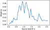 |
Fig. 1. Distribution of redshifts used to combine simulated convergence maps from the κTNG dataset. |
4.1.3. Noisy shear maps
In accordance with Eq. (1), to generate noisy shear maps γi from κi, we applied the inverse KS filter A and added a zero-mean Gaussian noise ni with a diagonal covariance matrix Σn shared among all calibration and test input images. Its diagonal values were obtained by binning the weak lensing shear catalog created by Schrabback et al. (2010) (referred to as “S10”, following Remy et al. 2023) at the κTNG resolution (0.29 arcmin per pixel) and then applying Eq. (A.14). The intrinsic standard deviation σell was estimated from the measured ellipticities and set to 0.28. This is a reasonable estimation, assuming that the shear dispersion is negligible with respect to the dispersion of intrinsic ellipticities. The corresponding number of galaxies per pixel is represented in Fig. 2.
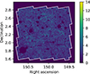 |
Fig. 2. Number of galaxies per pixel using the S10 weak lensing shear catalog (Schrabback et al. 2010). All redshifts have been considered. The white borders delimit the survey boundaries. Even within boundaries, some data are missing due to survey measurement masks. |
The S10 catalog is based on observations conducted by the NASA/ESA Hubble Space Telescope targeting the COSMOS field (Scoville et al. 2007) as well as photometric redshift measurements from Mobasher et al. (2007). It contains an average of 32 galaxies per square arcminute over a wide range of redshifts, which is consistent with what is expected from forthcoming surveys such as Euclid. This number excludes the galaxies with redshifts below 3.45 × 10⁻² and above 2.57 for the sake of consistency with the κTNG dataset. It also ignores the inactive pixels, k ∉ ℳ, without any observed galaxy. In these areas, we simply set the shear map values to zero, as explained in Appendix A.4. Consequently, we omitted these regions from our statistical analyses. An example of the simulated convergence map κi and the corresponding noisy shear map γi is provided in Fig. 3.
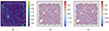 |
Fig. 3. Example of simulated convergence map (Fig. 3a) and the corresponding noisy shear map (Figs. 3b and 3c). (a) κi, (b) Re(γi), (c) Im(γi). |
4.1.4. Reconstruction parameters
The Wiener estimate  as well as the Gaussian component
  of MCALens were computed with a power spectrum (diagonal elements of Pκ) empirically estimated from a dataset of 180 simulated convergence maps distinct from the calibration and test sets. Moreover, the sparse component
  of MCALens was estimated using a starlet dictionary (Starck et al. 2007), which is well suited for isotropic objects. The detection threshold for selecting the set of active wavelet coefficients was set to 4σ. This threshold was selected based on visual evaluation, as it achieved a good balance between effectively detecting peaks and minimizing false positives. For both iterative methods, the number of iterations was set to the default value of 12. This choice was motivated by seeking a trade-off between reconstruction accuracy and computational cost. Finally, the KS maps were smoothed with a Gaussian filter S with a full width at half maximum (FWHM) of 2.4 arcmin, following Starck et al. (2021). To test the effect of the low-pass filter on reconstruction accuracy and error bar size, we also used a filter with half the original FWHM. These two degrees of filtering are referred to as strong and weak smoothing, respectively.
4.1.5. Uncertainty quantification parameters
We selected a target confidence level at 2σ corresponding to α ≈ 0.046. We notice that higher confidence levels require larger calibration sets due to the finite-sample correction: The CQR algorithm selects the (1 − α)(1 + 1/n)-th empirical quantile of the conformity scores, which by definition must remain below 100%. Consequently, a 2σ confidence requires at least n = 21 calibration samples, versus n = 370 at 3σ and n = 15 787 at 4σ. Moreover, regarding the approach based on RCPS, we tested three values for the error level: δ = 0.05, 0.2, and 0.5.
We implemented both approaches with several families of calibration functions, which represents a novel aspect of this work:

as used by Romano et al. (2019), and

as used by Angelopoulos et al. (2022a). The former increases (or decreases) the size of the confidence intervals by the same value λ regardless of the initial size 2r, whereas the latter adjusts the size proportionally to its initial value. This choice may have an influence on the average size of the calibrated confidence intervals. To push the analysis further, we also tested calibration functions with intermediate behaviors for the CQR approach in the form

where Fχ2(k) denotes the cumulative distribution function of a chi-squared distribution with k degrees of freedom, and a and b denote positive real numbers. In practice, we tested values of a ranging from 0.004 to 0.012, and we adjusted b to the maximum value such that gλ remains non-decreasing for any λ ≥ 0. In the rest of the paper, the functions defined in Eqs. (49), (50), and (51), for which a visual representation is provided in Fig. 4, are referred to as “additive”, “multiplicative”, and “chi-squared”, calibration functions.
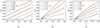 |
Fig. 4. Examples of families (gλ)λ of calibration functions. In Fig. 4a (additive calibration), λ ranges from −∞ to +∞ with λ0 = 0, whereas in Figs. 4b (multiplicative calibration) and 4c (chi-squared calibration), λ ranges from zero to +∞ with λ0 = 1. In Fig. 4c, the number k of degrees of freedom is set to three, the scaling factor a is set to 0.01, and the multiplicative factor b is set to the maximum value such that gλ remains non-decreasing for any λ ≥ 0, that is, b ≈ 0.041. (a) gλ : r ↦ max(r + λ, 0), (b) gλ : r ↦ λr, (c) gλ : r ↦ r + bFX2(k)(r/a)(λ − 1). |
4.2. Results
4.2.1. Visualization of reconstructed convergence maps
A visual example of a reconstructed convergence map together with its prediction bounds before and after calibration is provided in Fig. D.1. A focus on the main peak-like structure is displayed in Fig. 8 for the Wiener and MCALens estimates after calibration with CQR. One can observe that for the KS and Wiener methods, the high-density region (bright spot in the convergence map) falls outside the confidence bounds, even after calibration (it is actually underestimated). This is not in contradiction with the theoretical guarantees stated in Eqs. (29) and (45) because the expected miscoverage rate, computed across the whole set ℳ of active pixels, remains below the target α, as explained in Sect. 4.2.3. However, these guarantees do not reveal anything specific about the miscoverage rate of the higher-density regions. A more detailed discussion on this topic is provided in Sect. 5.3.
In contrast, MCALens correctly predicts the high-density region. This observation is consistent with the fact that this algorithm was designed to accurately reconstruct the sparse component of the density field.
4.2.2. Reconstruction accuracy
In order to reproduce previously established results, we measured for each i ∈ {n+1,…,m} in the test set the root mean square error (RMSE) between the ground truth κi and reconstructed convergence maps  ,
,  and
and  , which correspond to the KS, Wiener, and MCALens solutions, respectively. These metrics were computed on the set ℳ of active pixels, that is, within the survey boundaries, and for pixels with nonzero galaxies. We also measured the RMSE for high-density regions only, which are of greater importance when inferring cosmological parameters. More precisely, we only considered the pixels k such that |κi[k]| ≥ 4.8 × 10⁻², which corresponds to a signal-to-noise ratio above 0.25 (2.8% of the total number of pixels). The results are displayed in Table 1.
Reconstruction accuracy.
These results confirm that the Wiener and MCALens solutions achieve higher reconstruction accuracy compared to the KS solution, although the latter can be improved by increasing the standard deviation of the smoothing filter (see “KS1” versus “KS2”). Additionally, MCALens outperforms Wiener by 1.6%. This difference significantly increases when focusing on high-density regions (6.3% improvement).
4.2.3. Miscoverage rate
For each i ∈ {n+1,…,m} in the test set, we measured the empirical miscoverage rate  such as introduced in Eq. (35), where the (uncalibrated) lower- and upper-bounds
  and
and  were computed following Eq. (9), using each of the three reconstruction methods. Then, after calibrating the bounds using CQR and RCPS on the calibration set (γi, κi)i = 1n, we computed
  and
and  on the test set (γi, κi)i = n + 1m. Finally, we compared the results with the theoretical guarantees stated in Eqs. (34) and (45), respectively. The results are reported in Table D.1 and plotted in Fig. 5.
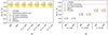 |
Fig. 5. Empirical miscoverage rate after calibration with CQR (Fig. 5a) and RCPS (Fig. 5b). The means and standard deviations were computed over the test set (γi, κi)i = n + 1m for various error levels δ (RCPS only) and various families of calibration functions (gλ)λ. More details are provided in the note of Table D.1. The theoretical bounds for CQR introduced in Eq. (34) are represented by the yellow area in Fig. 5a. These plots indicate that CQR achieves miscoverage rates that are, on average, close to the target α, whereas RCPS tends to produce overconservative bounds, even for large values of δ. (a) CQR, (b) RCPS. |
In the case of CQR, the empirical mean of the miscoverage rate falls between the theoretical bounds (yellow area). This is in line with the theoretical guarantee stated in Eq. (34). We also highlight that the lower bound seems overly conservative. It should be noted that the expected value from Eq. (34) covers uncertainties over not only the convergence map K and the noise N but also the calibration set (Γi, Ki)i = 1n. In our experiments, we only considered one realization (γi, κi)i = 1n of the calibration set, which, as explained in Sect. 3.4, may result in miscalibration and above target error rates. This effect could be mitigated by increasing the size n of the calibration set or with bootstrapping.
Unlike CQR, the RCPS approach controls the risk of picking a statistically deviant calibration set, which could lead to undercoverage by introducing an additional parameter δ. However, even with large values of δ, the calibrated bounds tend to be overly conservative. For example, with δ = 0.5, one would expect the average miscoverage rate to fluctuate around the target α in approximately 50% of experiments when repeating the protocol with different calibration sets. In practice, the computed miscoverage rates consistently fall well below the target. Contrary to CQR, RCPS does not prevent situations of overcoverage.
4.2.4. Mean length of prediction intervals
The mean length of the prediction intervals was computed over each image in the test set before and after calibration for each mass mapping method, each calibration method (CQR and RCPS), and each family of calibration functions. The results are reported in Table D.1 and plotted in Fig. 6.
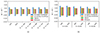 |
Fig. 6. Mean values for the lower and upper confidence bounds computed over the span of each image. The bar sizes represent the mean length of the error bars. As in Fig. 5, the values were computed over the test set (γi, κi)i = n + 1m for various families of calibration functions (gλ)λ. After calibration with CQR, the choice of mass mapping method does not influence the average miscoverage rate (Fig. 5a), but it does significantly affect the size of the error bars (Fig. 6a). Additionally, RCPS, which tends to produce overconservative prediction bounds (Fig. 5b), yields larger error bars than CQR (Fig. 6b vs 6a). (a) CQR, (b) RCPS. |
We observed that the choice of mass mapping method influences the size of the confidence intervals. Specifically, the KS solution yields larger calibrated error bars than either the Wiener or MCALens solutions, particularly in the weak-smoothing scenario (“KS1”). Additionally, the smallest confidence intervals were obtained with MCALens using CQR with the additive family of calibration functions (in bold in Table D.1). This family consistently produces equal or smaller confidence intervals compared to the multiplicative or chi-squared families for both CQR and RCPS calibration procedures. The modest improvement of the MCALens solution compared to the Wiener (0.24% reduction in the mean length) can be attributed to the overall similarity between the MCALens and Wiener outputs, with MCALens demonstrating higher reconstruction accuracy only in a few peak-like structures, which are essential for inferring cosmological parameters. Consequently, averaging the results over all pixels tends to hide essential properties of MCALens. A more detailed discussion on high-density regions is provided in Sect. 5.3.
As explained above, RCPS produces overly conservative bounds, which has a strong impact on the size of the confidence intervals. Smaller confidence intervals could be obtained by increasing the size n of the calibration set since the Hoeffding’s upper-confidence bound (38) decreases with increased values of n. Therefore, CQR seems more appropriate if the computational resources or available data are limited.
5. Discussion
5.1. Distribution-free versus Bayesian uncertainties
Extending distribution-free UQ to data-driven mass mapping methods (see Sect. 2.1) is straightforward provided one has access to a “first guess”, that is, an initial quantification of uncertainty. Such initial uncertainty bounds can be obtained following the Bayesian framework presented in Sect. 2.2.2, which provides theoretical guarantees similar to Eq. (47).
However, as explained in Sect. 2.2.3, this relies heavily on a proper choice of the prior distribution μ, and if the latter differs from the unknown oracle distribution μ*, the empirical mean of the miscoverage rate, computed over the test set, may significantly diverge from Eq. (47). Applying a post-processing calibration step, such as CQR or RCPS, allows the guarantees stated in Eq. (34) or (45), respectively, to be obtained. In these expressions, the expected value assumes K ∼ μ*, even though the underlying distribution μ* remains implicit – hence the term “distribution-free”. The only sufficient conditions for these properties to be satisfied are that the data from the calibration and test sets (Γi, Ki)i = 1m are exchangeable and that the conformity scores are almost surely distinct.
5.2. Beyond pixelwise uncertainty
This paper focuses on estimating error bars per pixel. While this approach is easily interpretable, it lacks some essential properties. First, it is important to consider the purpose of mass mapping and the type of information required. For instance, to infer cosmological parameters, several studies have proposed using peak counts (Kratochvil et al. 2010; Marian et al. 2013; Shan et al. 2014; Liu et al. 2015), convolutional neural networks that exploit information in the gradient around peaks (Ribli et al. 2019a,b), or neural compression of peak summary statistics (Jeffrey et al. 2021). Consequently, regions of higher density are of particular interest and should be treated with special attention.
In this context, alternative UQ schemes could be considered. Among these are the Bayesian hypothesis testing of structure (Cai et al. 2018a,b; Repetti et al. 2019; Price et al. 2021), which can assess whether a given structure in an image is a reconstruction artifact or has some physical significance. Additionally, a computationally efficient approach, based on wavelet decomposition and thresholding of the MAP reconstruction, has been recently proposed by Liaudat et al. (2024). This method estimates errors at various scales, highlighting the different structures of the reconstructed image. In fact, these ideas can be traced back to earlier work in the stochastic geometry literature (see, e.g., the book by Adler & Taylor 2007), including applications in neuroimaging (e.g., Fadili & Bullmore 2004). Another potential direction is the application of calibration procedures to blob detection (Lindeberg 1993), for which UQ methods have been recently developed by Parzer et al. (2023, 2024).
Another drawback of pixelwise UQ is that it does not account for correlations between pixels. For instance, whether a given pixel has been accurately predicted can impact the uncertainty bounds of the neighboring pixels, a property not reflected in per-pixel error bars. This concern intersects with the previous one, as it raises the question of correctly identifying the structures of interest in the reconstructed image, which typically span several pixels. To address this issue, Belhasin et al. (2024) propose applying UQ after decomposing the reconstructed images through principal component analysis. They also apply RCPS in this context, demonstrating that calibration methods can be used beyond the per-pixel framework.
5.3. Focus on higher-density regions
As confirmed by our experiments, CQR provides guarantees on the miscoverage rate  defined in Eq. (35). However, this score is computed by considering all active pixels k ∈ ℳ. This may hide disparities caused by latent factors such as the local density of the convergence field. To support this claim, we computed the miscoverage rate filtered on regions of higher density. More precisely, for any i ∈ {n+1,…,m}, we only considered pixels k such that |κi[k]| ≥ t for a given threshold t ∈ ℝ, set to 4.8 × 10⁻² in our experiments (S/N ratio above 0.25), similar to Sect. 4.2.2. The corresponding metric is defined by
![$$ \begin{aligned} L_{t}(\kappa ,\, \hat{\kappa }^{-},\, \hat{\kappa }^{+}) := \frac{ \text{ card}\,\Bigl \{ k \in \mathcal{M} _t(\kappa ) : \kappa [k] \notin \bigl [ \hat{\kappa }^{-}[k],\, \hat{\kappa }^{+}[k] \bigr ] \Bigr \} }{\text{ card}\mathcal{M} _t(\kappa )}, \end{aligned} $$](/articles/aa/full_html/2025/02/aa51756-24/aa51756-24-eq140.gif)
with
![$$ \begin{aligned} \mathcal{M} _t(\kappa ) := \Bigl \{ k \in \mathcal{M} : \kappa [k] \ge t \Bigr \}. \end{aligned} $$](/articles/aa/full_html/2025/02/aa51756-24/aa51756-24-eq141.gif)
The results, displayed in Fig. 7, indicate that the filtered miscoverage rate remains well above the target α, even after calibration with CQR. This phenomenon can also be visualized in Fig. 8 for the Wiener method, the bright area remains underestimated.
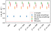 |
Fig. 7. Empirical miscoverage rate after calibration with CQR, computed on regions of higher density. Following Sect. 4.2.2, only pixels k with |κi[k]| ≥ t = 4.8 × 10⁻² were considered. Unlike in Fig. 5a, where the miscoverage rate is computed over all pixels, the measured values in this case deviate drastically from the target. Consequently, the size of the error bars is underestimated in these areas. |
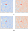 |
Fig. 8. Lower and upper bounds after calibration with CQR with a focus on a peak-like structure. (See Fig. D.1 for more details.) In the Wiener solution, the ground truth κ[k] remains above |
![$ {{\hat{{{{\kappa}}}}}^{+}}[k] $](/articles/aa/full_html/2025/02/aa51756-24/aa51756-24-eq142.gif)
As highlighted in Sect. 5.2, high-density regions are important for inferring cosmological parameters. Therefore, the method could be improved by explicitly prioritizing these regions. An interesting direction involves the conformal prediction masks introduced by Kutiel et al. (2023). This approach consists of masking the regions of low uncertainty in a given image, allowing for a focus on the regions of higher uncertainty – which correspond to high-density regions in the case of weak lensing mass mapping.
Figure 9 presents a scatter plot summarizing the various metrics discussed in this study.
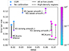 |
Fig. 9. Mean length of prediction intervals (Sect. 4.2.4) plotted against RMSE (Sect. 4.2.2) before and after calibration using additive CQR and with and without filtering on high-density regions. Marker colors indicate empirical miscoverage rates (Sect. 4.2.3). The coverage guarantee (34) applies only after calibration (blue diamonds atop the solid lines). We notice that when filtering on high-density regions, the coverage property no longer holds (pink diamonds atop the dashed lines). |
It indicates that Wiener and MCALens show a similar error bar size and RMSE when computed across the entire set ℳ of active pixels. From the perspective of these metrics, both methods outperform the KS estimators. However, when focusing on high-density regions, the Wiener solution exhibits poorer performance in terms of reconstruction accuracy (RMSE) and miscoverage rate compared to MCALens and KS. As a result, MCALens achieves a balance between overall and high-density specific performance. Additionally, the choice of smoothing filter significantly influences the reconstruction accuracy and error bar size of the KS estimator.
6. Conclusion
In this work, we emphasize the need for adjusting uncertainty estimates for reconstructed convergence maps, whether computed through frequentist or Bayesian frameworks. To address this, we built on two recent distribution-free calibration methods – CQR and RCPS – to obtain error bars with valid coverage guarantees.
This paper presents several key innovations. First, while RCPS has been applied to inverse problems in other contexts, CQR was originally designed for scalar regression and required adaptation for this specific application. Second, no prior work has compared the two methods directly. Finally, we investigated various families of calibration functions for both approaches.
Our experiments led to three key findings. First, RCPS tends to produce overconservative confidence intervals, whereas CQR allows for more accurate – and smaller – error bars. Second, the choice of mass mapping method significantly influences the size of these error bars: a 45% reduction for MCALens compared to KS with weak smoothing, a 14% reduction compared to KS with strong smoothing, and a 0.24% reduction compared to Wiener. Finally, this choice also affects the reconstruction accuracy, especially around peak-like structures, where MCALens outperforms Wiener by 6.3%. We emphasize that these calibration approaches are not limited to the model-driven mass mapping methods discussed in this paper; they are applicable to any mass mapping method, including those based on deep learning.
To conclude and guide future research, we acknowledge several limitations of this study. First, particular attention must be given to the intensity of peak-like structures, which are essential for inferring cosmological parameters. As it stands, neither of the two calibration methods effectively prevents miscoverage in these high-density regions. Additionally, this work could be expanded to include a broader range of uncertainty estimates beyond per-pixel error bars. Finally, the calibration and resulting uncertainty bounds were derived for a specific set of cosmological parameters. While we postulate that variations in cosmology have only a marginal impact on the results, this hypothesis needs further investigation.
Data availability
To ensure reproducibility, all software, scripts, and notebooks used in this study are available on GitHub, at https://github.com/hubert-leterme/weaklensing_uq.git.
This point estimate may differ from the one obtained in Eq. (17) within the Bayesian framework because the CQR algorithm presented in this paper requires equally sized lower and upper residuals. Although Romano et al. (2019) proposed an asymmetric version of their algorithm, it tends to increase the length of prediction intervals.
Acknowledgments
This work was funded by the TITAN ERA Chair project (contract no. 101086741) within the Horizon Europe Framework Program of the European Commission, and the Agence Nationale de la Recherche (ANR-22-CE31-0014-01 TOSCA and ANR-18-CE31-0009 SPHERES).
References
- Adler, R. J., & Taylor, J. E. 2007, in Random Fields and Geometry (Springer), Springer Monographs in Mathematics [Google Scholar]
- Angelopoulos, A. N., Kohli, A. P., Bates, S., et al. 2022a, in Proceedings of the 39th International Conference on Machine Learning (PMLR), 717 [Google Scholar]
- Angelopoulos, A. N., Bates, S., Malik, J., & Jordan, M. I. 2022b, in International Conference on Learning Representations [Google Scholar]
- Bates, S., Angelopoulos, A., Lei, L., Malik, J., & Jordan, M. 2021, J. ACM, 68, 43:1 [CrossRef] [Google Scholar]
- Belhasin, O., Romano, Y., Freedman, D., Rivlin, E., & Elad, M. 2024, IEEE Trans. Pattern Anal. Mach. Intell., 46, 3321 [Google Scholar]
- Bobin, J., Starck, J.-L., Sureau, F., & Fadili, J. 2012, Adv. Astron., 2012, e703217 [CrossRef] [Google Scholar]
- Boucheron, S., Lugosi, G., & Bousquet, O. 2004, in Advanced Lectures on Machine Learning (Springer), 208 [Google Scholar]
- Cai, X., Pereyra, M., & McEwen, J. D. 2018a, MNRAS, 480, 4154 [Google Scholar]
- Cai, X., Pereyra, M., & McEwen, J. D. 2018b, MNRAS, 480, 4170 [NASA ADS] [CrossRef] [Google Scholar]
- Durmus, A., Moulines, É., & Pereyra, M. 2018, SIAM J. Imaging Sci., 11, 473 [CrossRef] [Google Scholar]
- Fadili, M. J., & Bullmore, E. T. 2004, NeuroImage, 23, 1112 [CrossRef] [Google Scholar]
- Horwitz, E., & Hoshen, Y. 2022, arXiv e-prints [arXiv:2211.09795] [Google Scholar]
- Jeffrey, N., & Wandelt, B. D. 2020, in Third Workshop on Machine Learning and the Physical Sciences (NeurIPS 2020) [Google Scholar]
- Jeffrey, N., Lanusse, F., Lahav, O., & Starck, J.-L. 2020, MNRAS, 492, 5023 [Google Scholar]
- Jeffrey, N., Alsing, J., & Lanusse, F. 2021, MNRAS, 501, 954 [Google Scholar]
- Kaiser, N., & Squires, G. 1993, ApJ, 404, 441 [Google Scholar]
- Kilbinger, M. 2015, Rep. Prog. Phys., 78, 086901 [Google Scholar]
- Klatzer, T., Dobson, P., Altmann, Y., et al. 2024, SIAM J. Imaging Sci., 17, 1078 [CrossRef] [Google Scholar]
- Kratochvil, J. M., Haiman, Z., & May, M. 2010, Phys. Rev. D, 81, 043519 [Google Scholar]
- Kutiel, G., Cohen, R., Elad, M., Freedman, D., & Rivlin, E. 2023, in ICLR 2023 Workshop on Trustworthy Machine Learning for Healthcare [Google Scholar]
- Lanusse, F., Starck, J.-L., Leonard, A., & Pires, S. 2016, A&A, 591, A2 [NASA ADS] [CrossRef] [EDP Sciences] [Google Scholar]
- Laumont, R., Bortoli, V. D., Almansa, A., et al. 2022, SIAM J. Imaging Sci., 15, 701 [CrossRef] [Google Scholar]
- Lei, J., & Wasserman, L. 2014, J. R. Stat. Soc., B: Stat. Methodol., 76, 71 [CrossRef] [Google Scholar]
- Liaudat, T. I., Mars, M., Price, M. A., et al. 2024, RASTI, 3, 505 [NASA ADS] [Google Scholar]
- Lindeberg, T. 1993, Int. J. Comput. Vis., 11, 283 [CrossRef] [Google Scholar]
- Liu, J., Petri, A., Haiman, Z., et al. 2015, Phys. Rev. D, 91, 063507 [Google Scholar]
- Marian, L., Smith, R. E., Hilbert, S., & Schneider, P. 2013, MNRAS, 432, 1338 [Google Scholar]
- McEwen, J. D., Liaudat, T. I., Price, M. A., Cai, X., & Pereyra, M. 2023, arXiv e-prints [arXiv:2307.00056] [Google Scholar]
- Mobasher, B., Capak, P., Scoville, N. Z., et al. 2007, ApJS, 172, 117 [NASA ADS] [CrossRef] [Google Scholar]
- Narnhofer, D., Habring, A., Holler, M., & Pock, T. 2024, SIAM J. Imaging Sci., 17, 301 [CrossRef] [Google Scholar]
- Osato, K., Liu, J., & Haiman, Z. 2021, MNRAS, 502, 5593 [Google Scholar]
- Parzer, F., Jethwa, P., Boecker, A., et al. 2023, A&A, 674, A59 [NASA ADS] [CrossRef] [EDP Sciences] [Google Scholar]
- Parzer, F., Kirisits, C., & Scherzer, O. 2024, J. Math. Imaging Vis., 66, 697 [CrossRef] [Google Scholar]
- Pereyra, M. 2016, Stat. Comput., 26, 745 [CrossRef] [Google Scholar]
- Pereyra, M. 2017, SIAM J. Imaging Sci., 10, 285 [CrossRef] [Google Scholar]
- Pereyra, M., Mieles, L. V., & Zygalakis, K. C. 2020, SIAM J. Imaging Sci., 13, 905 [CrossRef] [Google Scholar]
- Price, M. A., Cai, X., McEwen, J. D., et al. 2020, MNRAS, 492, 394 [Google Scholar]
- Price, M. A., McEwen, J. D., Cai, X., et al. 2021, MNRAS, 506, 3678 [NASA ADS] [CrossRef] [Google Scholar]
- Remy, B., Lanusse, F., Jeffrey, N., et al. 2023, A&A, 672, A51 [NASA ADS] [CrossRef] [EDP Sciences] [Google Scholar]
- Repetti, A., Pereyra, M., & Wiaux, Y. 2019, SIAM J. Imaging Sci., 12, 87 [Google Scholar]
- Ribli, D., Pataki, B. Á., & Csabai, I. 2019a, Nat. Astron., 3, 93 [Google Scholar]
- Ribli, D., Pataki, B. Á., Zorrilla Matilla, J. M., et al. 2019b, MNRAS, 490, 1843 [CrossRef] [Google Scholar]
- Romano, Y., Patterson, E., & Candes, E. 2019, in Advances in Neural Information Processing Systems (Curran Associates, Inc.), 32 [Google Scholar]
- Romano, Y., Sesia, M., & Candes, E. 2020, in Advances in Neural Information Processing Systems (Curran Associates, Inc.), 33 [Google Scholar]
- Sadinle, M., Lei, J., & Wasserman, L. 2019, J. Am. Stat. Assoc., 114, 223 [CrossRef] [Google Scholar]
- Schrabback, T., Hartlap, J., Joachimi, B., et al. 2010, A&A, 516, A63 [CrossRef] [EDP Sciences] [Google Scholar]
- Scoville, N., Abraham, R. G., Aussel, H., et al. 2007, ApJS, 172, 38 [NASA ADS] [CrossRef] [Google Scholar]
- Shan, H., Kneib, J.-P., Comparat, J., et al. 2014, MNRAS, 442, 2534 [NASA ADS] [CrossRef] [Google Scholar]
- Shirasaki, M., Yoshida, N., & Ikeda, S. 2019, Phys. Rev. D, 100, 043527 [NASA ADS] [CrossRef] [Google Scholar]
- Shirasaki, M., Moriwaki, K., Oogi, T., et al. 2021, MNRAS, 504, 1825 [NASA ADS] [CrossRef] [Google Scholar]
- Starck, J.-L., Elad, M., & Donoho, D. 2005, IEEE Trans. Image Process., 14, 1570 [Google Scholar]
- Starck, J.-L., Fadili, J., & Murtagh, F. 2007, IEEE Trans. Image Process., 16, 297 [Google Scholar]
- Starck, J.-L., Donoho, D. L., Fadili, M. J., & Rassat, A. 2013, A&A, 552, A133 [NASA ADS] [CrossRef] [EDP Sciences] [Google Scholar]
- Starck, J.-L., Themelis, K. E., Jeffrey, N., Peel, A., & Lanusse, F. 2021, A&A, 649, A99 [NASA ADS] [CrossRef] [EDP Sciences] [Google Scholar]
- Steinwart, I., & Christmann, A. 2011, Bernoulli, 17, 211 [CrossRef] [MathSciNet] [Google Scholar]
- Takeuchi, I., Le, Q. V., Sears, T. D., & Smola, A. J. 2006, J. Mach. Learn. Res., 7, 1231 [Google Scholar]
- Teneggi, J., Tivnan, M., Stayman, W., & Sulam, J. 2023, in Proceedings of the 40th International Conference on Machine Learning (PMLR), 33940 [Google Scholar]
- Vovk, V., Gammerman, A., & Shafer, G. 2005, Algorithmic Learning in a Random World (Springer-Verlag) [Google Scholar]
Appendix A: Mass mapping: Problem formulation
The following formalism has been outlined by Kilbinger (2015).
A.1. Weak lensing and mass mapping
Consider a light ray emitted by an extended source (typically, a galaxy), observed at coordinates θ ∈ ℝ2 in the sky. In the presence of (inhomogeneous) matter density that we seek to estimate, the light ray undergoes continuous deflection as it travels through space, a phenomenon known as gravitational lensing. In the absence of lensing, it would be seen by the observer at coordinates β(θ). Assuming deflections are small enough (weak lensing regime), one can write
where ψ : ℝ2 → ℝ denotes a lensing potential. Now, consider another light ray emitted by the same galaxy, observed at coordinates θ + δθ. A first-order approximation yields

where the Jacobian J : ℝ2 → ℝ2 × 2 (also referred to as amplification matrix) satisfies

where we have introduced the fields κ, γ1, γ2 : ℝ2 → ℝ such that

and gi := γi/(1 + κ), i = 1, 2. For any θ ∈ ℝ2, κ(θ)∈ℝ, referred to as the convergence, translates into an isotropic dilation of the source, and γ(θ):=γ1(θ)+iγ2(θ)∈ℂ, referred to as the shear, causes anisotropic stretching of the image, typically transforming a circle into an ellipse. Finally, g(θ):=g1(θ)+ig2(θ) is referred to as the reduced shear.
The goal is now to estimate the projected mass between the observer and the observed galaxies in any direction. In the weak lensing regime, it can be shown that the convergence κ(θ) is roughly proportional to the (weighted) matter density projected along the line of sight between the observer and the source. Therefore, mass mapping can be performed by estimating the convergence map κ : ℝ2 → ℝ from the observation of galaxies at a given redshift.
A.2. Relationship between shear and convergence
Although not directly measurable, κ can be retrieved from the shear γ, up to an additive constant. In the flat sky limit, solving the PDEs (A.4) yields the following relationship in the Fourier space:
Denoting by ℱ the Fourier transform operator, this yields
Now, we discretize Eq. (A.6) on a square grid of size K2 ∈ ℕ, and adopt a vector-matrix notation in which the shear and convergence maps γ ∈ ℂK2 and κ ∈ ℝK2 are flattened and thus represented as one-dimensional vectors. By neglecting discretization and boundary effects, we get the following relation:

where F and its Hermitian transpose F* ∈ ℂK2 × K2 respectively encode the discrete Fourier and inverse Fourier transforms, and P ∈ ℂK2 × K2 is a diagonal matrix obtained by discretizing  on the same grid: for any (k1, k2)≠(0, 0),
![$$ \begin{aligned} \mathbf P \left[ K^2 k_1 + k_2,\, K^2 k_1 + k_2 \right] := \frac{(k_1 + i k_2)^2}{k_1^2 + k_2^2}. \end{aligned} $$](/articles/aa/full_html/2025/02/aa51756-24/aa51756-24-eq151.gif)
The constant γ0 := ⟨γ⟩∈ℂ (mean value of the shear map) accounts for the fact that  is discontinuous in 0, thereby leaving P[0, 0] undefined when discretizing (mass-sheet degeneracy). In practice, we therefore set P[0, 0] = 0 and add this constant to the equation.
Due to mass-sheet degeneracy, the operator A is not invertible. Therefore, assuming the shear map γ is known, the convergence map κ can only be retrieved up to an additive constant:

where κ0 := ⟨κ⟩∈ℝ denotes the mean value of the convergence map, and P† ∈ ℂK2 × K2 denotes a diagonal matrix defined by P†[0, 0]: = 0 and, for all k ≠ 0, by P†[k, k]:=P[k, k]−1. In practice, we will therefore estimate the variations of κ around its mean value.
A.3. Shear measurement
The intrinsic ellipticity of a galaxy is characterized by a complex number ϵs ∈ ℂ. In the weak lensing regime, the observed ellipticity ϵ approximately satisfies

where, as a reminder, g ∈ ℂ denotes the reduced shear, which varies with the galaxy coordinates θ. A common approximation in weak lensing is to consider κ ≪ 1, and therefore g ≈ γ. In the remainder of the section we replace g with the unreduced shear, γ. Assuming the intrinsic galaxy ellipticity has no preferred orientation, the expected value of ϵs vanishes, which yields 𝔼[ϵ]=𝔼[γ]. Therefore, the observed ellipticity ϵ is an unbiased estimator of γ.
In practice, a portion of the sky on which one seeks to perform mass mapping is considered, and subdivided into K2 small regions (or bins), each of which being associated to a pixel in the discretized shear map γ and convergence map κ. For each bin k, the ellipticity of Nk galaxies at a given redshift is measured. Then, Eq. (A.10) yields
where γk, i denotes the shear, and ϵk, i and ϵk, is respectively denote the intrinsic and measured ellipticity of the i-th galaxy within the k-th bin. Assuming that the bins are small enough to maintain an approximate constancy of the shear within each, we get
![$$ \begin{aligned} \frac{1}{N_{k}} \sum _{i=1}^{N_{k}} \gamma _{k,\, i} = \gamma [k]. \end{aligned} $$](/articles/aa/full_html/2025/02/aa51756-24/aa51756-24-eq156.gif)
Moreover, we introduce
![$$ \begin{aligned} \epsilon [k] := \frac{1}{N_{k}} \sum _{i=1}^{N_{k}} \epsilon _{k,\, i} \quad \text{ and}\quad n[k] := \frac{1}{N_{k}} \sum _{i=1}^{N_{k}} \epsilon ^s_{k,\, i}, \end{aligned} $$](/articles/aa/full_html/2025/02/aa51756-24/aa51756-24-eq157.gif)
in which ϵ is an unbiased estimator of γ, and n is the realization of a Gaussian noise with zero mean and diagonal covariance matrix Σn ∈ ℂK2 × K2, satisfying
![$$ \begin{aligned} \Sigma _{n}[k,\, k] = \sigma _{\text{ ell}} / \sqrt{N_{k}}, \end{aligned} $$](/articles/aa/full_html/2025/02/aa51756-24/aa51756-24-eq158.gif)
where σell ∈ ℂ denotes the standard deviation of the intrinsic ellipticities. In practice, this quantity is estimated by measuring the standard deviation of the observed ellipticities across the sky. In practice, the number of galaxies per bin may be quite small (Nk ∼ 10), which yields a very low S/N ratio.
Then, combining Eqs. (A.7) and (A.11)-(A.13) yields
Since the noise n has zero-mean, we have γ0 ≈ ⟨ϵ⟩. Therefore, by replacing the true unknown shear map by its unbiased estimator, and after applying mean-centering: γ := ϵ − ⟨ϵ⟩, we get the inverse problem stated in Eq. (1), for which we seek an estimation of the convergence map κ.
A.4. Masked data
In practice, some data may be missing due to survey measurement masks (for instance, limits of the galaxy survey or bright stars in the foreground). A naive approach to address this issue is to set γ[k] = 0 for any k ∉ ℳ, where

denotes the set of “active” pixels. Then, if we assign n[k] to −Aκ[k] outside ℳ, Eq. (1) still holds, but n can no longer be considered as a Gaussian noise. For the sake of simplicity, in this paper, we nevertheless relied on this solution, and assigned a very large noise variance Σn[k, k] for any k ∉ ℳ, which is required for the Wiener and MCALens mass mapping methods (see Sects. B.2 and B.3, respectively).
Another approach involves adding a Gaussian white noise n′ with large variance σ′2 to the masked pixels: γ[k]:=n′[k] for any k ∉ ℳ. Assuming the S/N ratio between Aκ and n′ is small enough, we therefore approximately get Eq. (1), where the noise variance is left unchanged for unmasked pixels, and is equal to σ′2 in masked regions.
Because of noise and masked data, this inverse problem is ill-posed. Therefore, mass-mapping methods generally rely on prior assumptions to regularize the problem.
Appendix B: Mass mapping methods
In this section we present the three mass mapping methods used in our experiments.
B.1. Kaiser-Squires inversion
The KS inversion (Kaiser & Squires 1993) consists in a simple pseudo-inversion of the linear operator A. According to Eq. (A.9), in absence of noise and mask, it provides an exact reconstruction of the true convergence map κ (up to an additive constant). In practice, it is generally followed by a certain amount of Gaussian smoothing:

where S ∈ ℝK2 × K2 encodes a Gaussian smoothing operator with manually tuned variance.
We note that in absence of smoothing (S = I), the KS solution corresponds to the maximum likelihood estimate of the convergence map:
where fΓ | K(γ | κ′) denotes the likelihood density.
B.2. Iterative Wiener filtering
The KS inversion generally produces poor results because it is very sensitive to noise and masked data. To overcome this limitation, one introduce prior assumptions in the form of a regularization term in the objective function. Considering κ as drawn from a random variable with probability density function p, the MAP estimate satisfies Eq. (19).
In the Wiener approach, κ is considered as a Gaussian field. That is, it is drawn from a multivariate Gaussian distribution with (non-diagonal) covariance matrix Σκ, and the covariance matrix of its Fourier transform  , denoted by Pκ := FΣκF*, is diagonal. Then, the distribution from which κ is drawn is entirely characterized by its power spectrum. In this context, Eq. (19) becomes
By setting the gradient of the above expression to 0, we get

If the noise is not stationary, then computing Eq. (B.5) requires two K2 × K2-matrix inversions, which is not feasible in practice. To overcome this, Bobin et al. (2012) proposed an iterative algorithm converging toward Eq. (B.5), in the context of cosmic microwave background (CMB) map restoration. Each iteration consists in a two-step process: one step in the spatial domain and one step in the Fourier domain. The algorithm takes advantage of the fact that the covariance matrices Σn and Pκ are diagonal, thereby avoiding large matrix inversions.
B.4. MCALens algorithm
In contrast to the CMB, matter distribution is actually poorly approximated by Gaussian fields, due to the gravitational interactions responsible for the formation of galaxies and large-scale structures. In a more recent paper, Starck et al. (2021) suggested that convergence maps can be represented as the superposition of a Gaussian component, as in the Wiener solution, and a sparse component in a wavelet dictionary, as in GLIMPSE2D:
The authors then proposed to use the morphological component analysis (MCA) algorithm (Starck et al. 2005), considering that the Gaussian and sparse components are morphologically distinct (except for lower frequencies). They came along with an iterative algorithm called MCALens, where each iteration is a two-step process. First, perform one iteration of the GLIMPSE2D algorithm on the residual  , and update the sparse component
  . Then, perform one iteration of Wiener filtering, described in Sect. B.2, on the residual
  , and update the Gaussian component
  . Finally, since we can only estimate the variations of the convergence around its mean value, the output of the MCALens algorithm undergoes mean centering.
Appendix C: Proof of Proposition 1
The exchangeability of (Xi, Yi)i = 1n + 1 implies the exchangeability of the conformity scores  . Moreover, by hypothesis, the latter are almost surely distinct. Therefore, we can apply Lemma 2 by Romano et al. (2019, supplementary material):
where we have denoted Λ := Λn + 1. Let λ and λ(α) denote realizations of Λ and Λ(α), respectively. Then, λ corresponds to the (unknown) conformity score associated with the outcome (x, y) of (X, Y). It satisfies, similarly to Eqs. (26)-(27),
![$$ \begin{aligned} \lambda&= \min \left\{ \lambda ^{\prime } \in \left[a,\, b\right] :\, y \in \hat{\mathcal{C} }_{\lambda ^{\prime }}(x) \right\} \end{aligned} $$](/articles/aa/full_html/2025/02/aa51756-24/aa51756-24-eq174.gif)
![$$ \begin{aligned}&= \min \left\{ \lambda ^{\prime } \in \left[a,\, b\right] :\, g_{\lambda ^{\prime }}\bigl (\hat{r}(x)\bigr ) \ge \left| \hat{f}(x) - y \right| \right\} . \end{aligned} $$](/articles/aa/full_html/2025/02/aa51756-24/aa51756-24-eq175.gif)
Then, combining Eqs. (C.2), (C.3) and (24) yields, for any λ′∈ℝ,
Therefore, using λ′:=λ(α), we get
Finally, plugging Eq. (C.6) into Eq. (C.1) yields Eq. (29), which concludes the proof.
Appendix D: Detailed visualizations and results
Comprehensive visualizations of mass estimates and their uncertainties are shown in Fig. D.1, while detailed numerical results are provided in Table D.1.
UQ metrics: Miscoverage rate and mean length of prediction intervals.
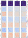 |
Fig. D.1. Top row: Point estimate, |


All Tables
All Figures
|
Fig. 1. Distribution of redshifts used to combine simulated convergence maps from the κTNG dataset. |
| In the text | |
|
Fig. 2. Number of galaxies per pixel using the S10 weak lensing shear catalog (Schrabback et al. 2010). All redshifts have been considered. The white borders delimit the survey boundaries. Even within boundaries, some data are missing due to survey measurement masks. |
| In the text | |
|
Fig. 3. Example of simulated convergence map (Fig. 3a) and the corresponding noisy shear map (Figs. 3b and 3c). (a) κi, (b) Re(γi), (c) Im(γi). |
| In the text | |
|
Fig. 4. Examples of families (gλ)λ of calibration functions. In Fig. 4a (additive calibration), λ ranges from −∞ to +∞ with λ0 = 0, whereas in Figs. 4b (multiplicative calibration) and 4c (chi-squared calibration), λ ranges from zero to +∞ with λ0 = 1. In Fig. 4c, the number k of degrees of freedom is set to three, the scaling factor a is set to 0.01, and the multiplicative factor b is set to the maximum value such that gλ remains non-decreasing for any λ ≥ 0, that is, b ≈ 0.041. (a) gλ : r ↦ max(r + λ, 0), (b) gλ : r ↦ λr, (c) gλ : r ↦ r + bFX2(k)(r/a)(λ − 1). |
| In the text | |
|
Fig. 5. Empirical miscoverage rate after calibration with CQR (Fig. 5a) and RCPS (Fig. 5b). The means and standard deviations were computed over the test set (γi, κi)i = n + 1m for various error levels δ (RCPS only) and various families of calibration functions (gλ)λ. More details are provided in the note of Table D.1. The theoretical bounds for CQR introduced in Eq. (34) are represented by the yellow area in Fig. 5a. These plots indicate that CQR achieves miscoverage rates that are, on average, close to the target α, whereas RCPS tends to produce overconservative bounds, even for large values of δ. (a) CQR, (b) RCPS. |
| In the text | |
|
Fig. 6. Mean values for the lower and upper confidence bounds computed over the span of each image. The bar sizes represent the mean length of the error bars. As in Fig. 5, the values were computed over the test set (γi, κi)i = n + 1m for various families of calibration functions (gλ)λ. After calibration with CQR, the choice of mass mapping method does not influence the average miscoverage rate (Fig. 5a), but it does significantly affect the size of the error bars (Fig. 6a). Additionally, RCPS, which tends to produce overconservative prediction bounds (Fig. 5b), yields larger error bars than CQR (Fig. 6b vs 6a). (a) CQR, (b) RCPS. |
| In the text | |
|
Fig. 7. Empirical miscoverage rate after calibration with CQR, computed on regions of higher density. Following Sect. 4.2.2, only pixels k with |κi[k]| ≥ t = 4.8 × 10⁻² were considered. Unlike in Fig. 5a, where the miscoverage rate is computed over all pixels, the measured values in this case deviate drastically from the target. Consequently, the size of the error bars is underestimated in these areas. |
| In the text | |
|
Fig. 8. Lower and upper bounds after calibration with CQR with a focus on a peak-like structure. (See Fig. D.1 for more details.) In the Wiener solution, the ground truth κ[k] remains above |
| In the text | |
|
Fig. 9. Mean length of prediction intervals (Sect. 4.2.4) plotted against RMSE (Sect. 4.2.2) before and after calibration using additive CQR and with and without filtering on high-density regions. Marker colors indicate empirical miscoverage rates (Sect. 4.2.3). The coverage guarantee (34) applies only after calibration (blue diamonds atop the solid lines). We notice that when filtering on high-density regions, the coverage property no longer holds (pink diamonds atop the dashed lines). |
| In the text | |
|
Fig. D.1. Top row: Point estimate, |
| In the text | |
Current usage metrics show cumulative count of Article Views (full-text article views including HTML views, PDF and ePub downloads, according to the available data) and Abstracts Views on Vision4Press platform.
Data correspond to usage on the plateform after 2015. The current usage metrics is available 48-96 hours after online publication and is updated daily on week days.
Initial download of the metrics may take a while.