| Issue |
A&A
Volume 694, February 2025
|
|
|---|---|---|
| Article Number | A42 | |
| Number of page(s) | 17 | |
| Section | Galactic structure, stellar clusters and populations | |
| DOI | https://doi.org/10.1051/0004-6361/202451672 | |
| Published online | 31 January 2025 | |
The supermassive black hole population from seeding via collisions in nuclear star clusters
1
Dipartimento di Fisica, Sapienza Università di Roma,
Piazzale Aldo Moro 5,
00185
Rome,
Italy
2
Departamento de Astronomía, Facultad Ciencias Físicas y Matemáticas, Universidad de Concepción, Av. Esteban Iturra s/n Barrio Universitario,
Casilla 160-C,
Concepción,
Chile
3
Carnegie Observatories,
813 Santa Barbara Street,
Pasadena,
CA
91101,
USA
4
Departamento de Astronomía, Universidad de Chile,
Casilla 36-D
Santiago,
Chile
5
Astronomisches Rechen-Institut, Zentrum für Astronomie, University of Heidelberg,
Mönchhofstrasse 12–14,
69120
Heidelberg,
Germany
★ Corresponding author; mliempi2018@udec.cl
Received:
26
July
2024
Accepted:
20
December
2024
The coexistence of nuclear star clusters (NSCs) and supermassive black holes (SMBHs) in galaxies with stellar masses of ∼1010 M⊙, scaling relations between their properties and the properties of the host galaxy (e.g., MNSCstellar − Mgalaxystellar and MBH − Mgalaxystellar), and the fact that NSCs seem to take on the role of SMBHs in less massive galaxies (and vice versa in the more massive ones) suggest that the origin of NSCs and SMBHs is related. In this study we implemented an ‘in situ’ NSC formation scenario in which NSCs are formed in the center of galaxies due to star formation in the accumulated gas. We explored the impact of the free parameter Ares, which regulates the amount of gas transferred to the NSC reservoir and thus plays a crucial role in shaping the cluster’s growth. Simultaneously, we included a black hole (BH) seed formation recipe based on stellar collisions within NSCs in the semi-analytic model GALACTICUS to explore the resulting population of SMBHs. We determined the parameter space of the NSCs that form a BH seed and find that in initially more compact NSCs, the formation of these BH seeds is more favorable. This leads to the formation of light, medium, and heavy BH seeds, which eventually reach masses of up to ∼109 M⊙ and is comparable to the observed SMBH mass function at masses above 108 M⊙ . Additionally, we compared the resulting population of NSCs with a NSC mass function derived from the stellar mass function of galaxies from the GAMA survey at ɀ < 0.06, finding a good agreement in terms of shape. We also find a considerable overlap in the observed scaling relations between the NSC mass, the stellar mass of the host galaxy, and the velocity dispersion, which is independent of the value of Ares . However, the chi-square analysis suggests that the model requires further refinement to achieve better quantitative agreement.
Key words: galaxies: evolution / galaxies: formation / galaxies: nuclei / quasars: supermassive black holes
© The Authors 2025
 Open Access article, published by EDP Sciences, under the terms of the Creative Commons Attribution License (https://creativecommons.org/licenses/by/4.0), which permits unrestricted use, distribution, and reproduction in any medium, provided the original work is properly cited.
This article is published in open access under the Subscribe to Open model. Subscribe to A&A to support open access publication.
1 Introduction
Observations show that nuclear star clusters (NSCs) and/or supermassive black holes (SMBHs) are nearly ubiquitous in the centers of galaxies (Seth et al. 2008a; Graham & Spitler 2009; Neumayer et al. 2011; Neumayer & Walcher 2012; Nguyen et al. 2019). Although the coexistence of the two objects is observed in almost all galaxies with stellar masses  (Filippenko & Ho 2003; González Delgado et al. 2008; Seth et al. 2008b; Neumayer et al. 2020), more massive galaxies tend to host only SMBHs (Kormendy & Ho 2013) and less massive galaxies only NSCs. Sometimes, therefore, the term central massive object is used when both types of objects are present in the host galaxy (Ferrarese et al. 2006).
It is interesting that NSCs and SMBHs follow similar scaling relations with the host-galaxy properties (see, e.g., Wehner & Harris 2006; Georgiev et al. 2016), which suggests that the two undergo similar physical process during their formation and evolution. By way of illustration, previous works explored the  correlation (Balcells et al. 2003; Scott & Graham 2013; den Brok et al. 2015; Sánchez-Janssen et al. 2019; Georgiev et al. 2016), which is also observed for SMBHs as
  (Ding et al. 2020; Tanaka et al. 2024), and other correlations between
  , and host galaxy luminosity or stellar velocity dispersion (Seth et al. 2008a; Gültekin et al. 2009a; Kormendy & Ho 2013).
The formation mechanisms of the two objects are still unclear. However, there are different models that explain the environmental conditions from which they form.
Two principal models have been proposed to explain the formation of NSCs in the center of galaxies: (i) the infall of globular clusters (GCs) into the nucleus due to dynamical friction and consecutive mergers in the center that build up a NSC (Tremaine et al. 1975; Capuzzo-Dolcetta 1993; Agarwal & Milosavljević 2011; Antonini 2013; Gray et al. 2024), thereby explaining the deficit of massive GCs in the inner part of the nucleated early-type galaxies (Lotz et al. 2001; Capuzzo-Dolcetta & Mastrobuono-Battisti 2009); and (ii) ‘in situ’ star formation in the galactic nucleus, which happens when gas reaches the center of the galaxy and NSCs are directly formed there (Loose et al. 1982; Antonini et al. 2015).
The mechanism that drives the gas to the central parsecs of the galaxy is not well understood. There are several possible processes that can cause the accumulation of gas in the center of galaxies: (i) bar-driven gas infall due to a non-axisymmetric potential reaching the central parsec (e.g., Shlosman et al. 1990); (ii) the dissipative nucleation scenario, in which the repeated merging of massive stellar and gaseous clumps developed from nuclear gaseous spiral arms as a consequence of the local gravitational instability leads to the accumulation of stars and gas in the nucleus (Bekki et al. 2006; Bekki 2007); (iii) tidal forces in flat galaxies without NSCs act on the gas in 0.1% of the effective radius of the galaxy, causing gas infall (Emsellem & van de Ven 2008); and (iv) the magnetorotational instability of the disk composed of neutral gas under the effect of a weak magnetic field causes a radial gas transport toward the nucleus (Milosavljević 2004).
As for NSCs, different pathways have been proposed to explain the formation of SMBHs (e.g., Rees 1984; Volonteri 2010; Woods et al. 2019; Inayoshi et al. 2020). From observations of quasars at different redshifts we can conclude that the first black holes (BHs) must have formed in the early Universe. A direct example is the quasar survey of Bañados et al. (2016), which contains more than 100 quasars at 5.6 ≲ ɀ ≲ 6.7, when the Universe was about 1 Gyr old. Fan et al. (2023) recently published a similar review but with the quasar redshift frontier extended to ɀ ~ 7.6, including more than 300 quasars.
One possible mechanism to explain the existence of such SMBHs is the formation of light BH seeds from stellar remnants. If those seeds accrete at the Eddington rate with a standard efficiency, ϵ ≈ 0.1, it would take at least 0.5 Gyr to reach ~109 M⊙ (Volonteri 2010). However, the James Webb Space Telescope (JWST)1 recently detected a luminous galaxy at ɀ = 10.6 that hosts a SMBH of 106.2 M⊙ that accretes at about five times the Eddington rate (Maiolino et al. 2024). This provides strong evidence for the early formation of SMBHs and supports the idea that SMBHs are the results of the evolution of heavy BH seeds.
There are different ways to form more massive seeds: (i) the direct collapse of a massive metal-free gas cloud can lead to the formation of “heavy” BH seeds with masses on the order of ~105 M⊙ (Rees 1984; Volonteri & Rees 2005; Ferrara et al. 2014; Latif & Schleicher 2015; Regan & Downes 2018); (ii) the formation of light and medium seeds as remnants of Population III stars (Haiman 2004; Whalen & Fryer 2012; Latif et al. 2013, 2014; Riaz et al. 2022; Singh et al. 2023); and (iii) the formation and growth of BHs within dense NSCs due to runaway star collisions (Begelman & Rees 1978; Quinlan & Shapiro 1987; Ebisuzaki 2003; Miller & Hamilton 2002; Portegies Zwart & McMillan 2002; Portegies Zwart et al. 2004; Gürkan et al. 2004; Freitag et al. 2006a,b; Escala 2021; Vergara et al. 2023). Even though the detection of NSCs in nearby galaxies is usually done through the analysis of the galaxy light profile, the detection of BHs within NSCs requires indirect methods such as kinematic measurements of the orbits of the stars and/or gas near the BH. One such example is the detection of the NSC (Becklin & Neugebauer 1968) in the Milky Way, after which the presence of Sagittarius A* was inferred 6 years later (Balick & Brown 1974).
In this work, we studied the expected population of SMBHs from the collision-based BH seeding scenario utilizing the semi-analytic model (SAM) for galaxy formation and evolution GALACTICUS (Benson 2012). The advantage of SAMs is the fast exploration of the parameter space (Henriques et al. 2009; Benson & Bower 2010; Bower et al. 2010) with low computational cost compared to N-body and/or hydrodynamical simulations. Of course, the degree of approximation depends on the implemented physics, but a good overall agreement can be achieved between semi-analytic and N-body and hydrodynamical models (Benson et al. 2001; Hirschmann et al. 2012; Côté et al. 2018; Mitchell et al. 2018). In Sect. 2 we describe the implementation and the methodology of our study, where in Sect. 2.1 we describe the NSC model implemented in GALACTICUS and in Sect. 2.2 the implementation of the BH seed formation scenario. We compare our results with the observed data and summarize our findings in Sect. 3. A final discussion and conclusions are provided in Sect. 4.
2 Methods
We used the SAM GALACTICUS2 developed by Benson (2012). The functionality of GALACTICUS is similar to other SAMs – for example GALFORM (Cole et al. 2000), L-GALAXIES (Henriques et al. 2015), and SAGE (Croton et al. 2016) – with the advantage that GALACTICUS is highly modular. This key feature allows a rapid incorporation of new models related to galaxy formation and evolution processes as this field is constantly evolving.
In this work we built a distribution of dark matter (DM) merger trees in GALACTICUS using the algorithm from Cole et al. (2000), which uses a modified version of the extended Press-Schechter formalism and the branching probabilities for the merger rates of DM halos (Parkinson et al. 2008; Benson 2017). The masses of the DM halos at ɀ = 0 are distributed uniformly from a power law mass distribution within the range 3.0 × 10⁹–1.1 × 10¹⁵ M⊙ calibrated to match the suite of MultiDark Planck cold DM N-body simulations3. To assure the resulting distribution of halo masses is representative of the expected halo mass function, GALACTICUS assigns a weight for each merger tree generated, allowing us to construct corrected, volume-limited samples.
The properties of DM halos are evolved forward in time until the mass resolution is reached; then the DM halos are populated with galaxies that are evolved over time in a Λ cold DM Universe with cosmological parameters equal to H0 = 67.36 km s−1 Mpc−1, Ωb = 0.0493, ΩΛ = 0.6847 and Ωm = 0.266 (Planck Collaboration X 2020). We adopted a mass resolution equals to 4.86 × 10⁵ M⊙. We discuss the convergence of the solutions due to the mass resolution in Appendix A.
Furthermore, our simulations are based on the best match parameters constrained with observations. We use the term “best-match parameters” to indicate the combination of parameters that best reproduces the observed datasets, for example the stellar mass-halo mass relation of Leauthaud et al. (2012), the ɀ < 0.06 stellar mass function of galaxies from the galaxy and mass assembly (GAMA) survey (Baldry et al. 2012), the ɀ = 2.5–3.0 stellar mass function of galaxies from the ultra deepsurvey with the visible and infrared survey telescope for astronomy telescope ULTRAVISTA survey (Muzzin et al. 2013), and the ɀ ≅ 0.00 BH mass-bulge mass relation (Kormendy & Ho 2013). For a comprehensive description of the target datasets used to constrain the model, we encourage readers to read the work of Knebe et al. (2018).
We emphasize that the primary aim of this paper is to introduce a new model for NSC (and BH) formation and evolution within Galacticus, and explore the parameter space of NSCs that formed a BH seed under the proposed scenario. We also provide a brief comparison between the observed and predicted galaxy stellar mass functions in Appendix B. However, we emphasize also the preliminary nature of this comparison, considering the complex processes that contribute to the formation and evolution of NSCs and the formation of BHs within them. The comparison thus predominantly serves to determine whether the contribution is potentially relevant. For this purpose, we ran a grid of parameters, as detailed in Table 1, that we introduce jointly with the implementation in Sect. 2.1.
2.1 Nuclear star cluster formation model
We assumed an in situ star formation scenario in the gas accumulated in the center of the galaxies, which is particularly well justified for galaxies with stellar masses above 3 × 10¹¹ M⊙ (Antonini et al. 2015). The gas mass accumulation rate in the reservoir is correlated to the star formation rate (SFR) in the bulge (Granato et al. 2004; Haiman et al. 2004; Neumayer et al. 2011; Lapi et al. 2014; Antonini et al. 2015) and is given by
 (1)
(1)
where  is the SFR in the spheroidal component of the galaxy and Ares is a free parameter previously reported on the order of 10−2 −10−3 (Antonini et al. 2015).
The size of the NSC scales with the square root of the dynamical mass of the system. This assumption is motivated by the size-luminosity (mass) scaling relation of the observed NSCs (Antonini & Perets 2012; Antonini 2013),
 (2)
(2)
where r0 is the mean radius of the observed NSCs set to r0 = 3.3 pc (Neumayer et al. 2020), and  is the dynamical mass of the system.
To model the mass distribution of the NSCs, we assumed a Sérsic profile (Sérsic 1963) with index n = 2.28. This was motivated by the results of Pechetti et al. (2020), who analyzed density profiles for 29 galaxies containing NSCs in a volume-limited survey.
The SFR of the NSC is assumed to follow the law from Krumholz et al. (2009). The star formation occurs in a “quiescent” mode, takes place on a timescale tSF, as described by Krumholz et al. (2009), Sesana et al. (2014), and Antonini et al. (2015), and involves only a fraction of the cold gas ( fc) available for star formation:
 (3)
(3)
The fraction of cold gas available to form stars depends on the metallicity of the gas. At high metallicities (Z > 0.01 Z⊙) the fraction is determined by the molecular gas. On the other hand, at lower metallicities (Z < 0.01 Z⊙), star formation takes place in the atomic phase (Krumholz 2012) and
![${f_c} = \max \left( {2\% ,1 - {{\left[ {1 + {{\left( {{3 \over 4}{s \over {1 + \delta }}} \right)}^{ - 5}}} \right]}^{ - 1/5}}} \right),$](/articles/aa/full_html/2025/02/aa51672-24/aa51672-24-eq12.png) (4)
(4)


The timescale (tSF) is obtained assuming that star formation happens in clouds (Krumholz et al. 2009; Sesana et al. 2014; Antonini et al. 2015) and is given by
 (10)
(10)
where Σth = 85 M⊙ pc−2.
Finally, we estimated the age of the system (tH) using the mass weighted age due to the fact that young stars outshine older stars. This is a reasonable choice as the luminosity of NSCs is dominated by the light of the younger stars of the system (Boeker et al. 2003; Walcher et al. 2006; Dametto et al. 2014). The expression used to compute the age is given by the integral of the SFR of the NSC:
 (11)
(11)
where t is the present time and  is the SFR of the NSC at time t′.
Initial parameters for our SAM.
2.2 Black hole formation and evolution model
As already mentioned, the formation pathway of SMBHs is still unclear. Here in this paper we focus on the exploration of the formation pathway via collisions in NSCs, as motivated by the study of Escala (2021), who find that the observed NSCs are in a regime where collisions are not relevant over timescales corresponding to the lifetime of the system while well-resolved observed SMBHs are found in regimes where collisions are expected to be dynamically important, suggesting that SMBHs are formed from failed NSCs with average collision timescale shorter than the age of the system (tcoll ≤ tH). In the following subsections, we describe the different ingredients of our model.
2.2.1 Black hole seeding: Collision timescale and critical mass
The formation of a massive BH within dense stellar clusters has been discussed for a long time (e.g., Begelman & Rees 1978; Portegies Zwart & McMillan 2002; Glebbeek et al. 2009; Di Carlo et al. 2021). It is possible to estimate the collision timescale tcoll in any system with a large number of particles (Binney & Tremaine 2008). The expression is
 (12)
(12)
where λ is the mean free path and σ is the characteristic velocity dispersion. The mean free path can be probabilistically defined as
 (13)
(13)
where n is the number density of stars and Σ0 is the effective cross section (Landau et al. 1980). The velocity dispersion of a virialized NSC is  , with
  the stellar mass of the NSC, rNSC the radius of the NSC, and G the gravitational constant. If the NSC is composed of equal-mass stars with mass M⋆, and assuming a uniform distribution, the number density is
  . This allows us to rewrite the collision timescale as follows:
 (14)
(14)
where tcoll depends on the effective cross section (Σ0), given by  , with R⋆ the radius of a single star, and Θ is the Safronov number (Binney & Tremaine 2008):
 (15)
(15)
It is possible to define a critical mass (Mcrit) as the mass for which the collision timescale becomes equal to the age of the system (tcoll = tH), assuming stellar velocities correspond to virial equilibrium (Vergara et al. 2023):
 (16)
(16)
It was numerically determined by Vergara et al. (2023) that even in systems where trelax ≤ tcoll a significant fraction (10–50%) of the final cluster mass is turned into a central massive object, when the ratio of cluster mass over critical mass is of order 1 (i.e., for systems with collision timescale on the order of the age of the system).
We included an efficiency parameter, ϵr, to rescale the radius rNSC as rNSC → ϵrrNSC, with 0 < ϵr ≤ 1, and study the critical mass of initially more compact NSCs. This is motivated by observational and computational studies of young massive star clusters with initial sizes of less than 0.3 pc that can expand by more than a factor of 10 over the course of their evolution (Banerjee & Kroupa 2017). Additionally, we assumed our NSCs are composed of Sun-like stars (M⋆ = 1 M⊙ and R⋆ = 1 R⊙).
2.2.2 Implementation of the black hole seeding and its evolution in GALACTICUS
In the standard implementation of GALACTICUS, it is assumed that each galaxy contains an initial mass BH with mass M• specified in the initial parameter file. As in this study we aim to explore the consequences of a physically motivated, collision based BH formation recipe, we fixed the initial BH mass as M• = 10 M⊙ but did not allow it to accrete gas until a new BH seed is created due to stellar collisions within NSCs, with the new seed then replacing the previous one.
A new BH seed in the center of the galaxy is formed if the stellar mass of the NSC is larger than the critical mass  , and the stellar mass of the NSC is larger than a mass threshold,
  , introduced to avoid the collapse of nonphysical NSCs, as the concept of the critical mass implicitly assumes that the stellar cluster is well sampled, and we assumed here that it requires a minimum of around 1000 stars. The mass of the newly formed seed is
 (17)
(17)
where ϵ• = 0.5 is a free efficiency parameter. We note that each NSC is allowed to form only one BH seed (unless it undergoes a galaxy merger). The new BH seed merges with the initial seed and starts to accrete gas from a radiatively efficient thin disk as described by Shakura & Sunyaev (1973). Thereupon the accretion is given by
 (18)
(18)
where ϵrad is the radiative efficiency of the accretion flow, ϵjet is the efficiency by which accretion power is converted to jet power, and Ṁ0 is the rest mass accretion rate computed assuming Bondi–Hoyle–Lyttleton accretion (Edgar 2004).
For our accretion disk model, the ϵrad term is computed assuming that material falls into the BH without further energy loss from the innermost stable circular orbit. The explicit equation is
 (19)
(19)
where EISCO is the specific energy (computed internally by GALACTICUS in physical or gravitational units) of the BH. The jet power (ϵjet) is computed using the expressions (4) and (5) from Meier (2001). We used Eq. (4) for (Schwarzschild) low spin BHs and Eq. (5) for (Kerr) high spin BHs.
The rest mass accretion rate considers the contribution from the spheroid, the circumgalactic medium (CGM), and the NSC component, where each component is enhanced by a factor α. The expression is given by
 (20)
(20)
where α is equal to 5 for the spheroid and the NSC, and 6 for the CGM. Our Bondi–Hoyle–Lyttleton accretion model assumes a stationary accreting BH in a static uniform gaseous medium, which implies that the relative velocity is v = 0 km s−1, and the sound speed of the gas must be estimated. In order to estimate the sound speed, the gas of all the components is assumed to follow the ideal gas law. For the spheroidal component, the assumed temperature is Tspheroid = 100 K due to the absence of significant heating mechanisms. The temperature of the gas in the NSC component has been estimated to be around TNSC = 100 K (Tielens 2010) from observations. Finally, we computed the temperature of the CGM assuming an isothermal profile for the halo with the temperature equal to the virial temperature. This allowed us to estimate cs as
 (21)
(21)
with k the Boltzmann constant, T the temperature of the gas and m the mean mass of a single molecule.
3 Results
In this section, we present the results of the simulations listed in Table 1 and provide a comparison with observational results. First we explore the obtained scaling relations with the host galaxy in Sect. 3.1. In Sect. 3.2, we discuss the NSC mass function predicted with GALACTICUS and the observed ones. In Sect. 3.3, we analyze the properties of the NSCs that satisfied the conditions to form a BH seed under this scenario within. We present the resulting BH mass function in Sect. 3.4.
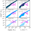 |
Fig. 1 Stellar mass of the NSCs as a function of the stellar mass of the galaxy (left) and as a function of the stellar velocity dispersion of the galaxy (right) for models A1, D1, and G1. Magenta dots correspond to observed NSCs following Table 3 of Neumayer et al. (2020); we removed galaxies whose stellar mass is not included and included the stellar velocity dispersion available in the literature. Magenta dots correspond to galaxies where the stellar mass of the NSC is well determined, while magenta triangles represent an upper limit instead. The corresponding table is available in Appendix D. Each panel includes the chi-squared test value of the model for reference. |
3.1 Nuclear star clusters and host galaxies
In this subsection, we analyze the properties of NSCs hosted in galaxies with  . In Fig. 1 we provide the stellar masses of NSCs as a function of the stellar mass of the host galaxy and as a function of the velocity dispersion of the bulge. For this purpose, we focused on models A1, D1, and G1, corresponding to values of Ares = 10−1,10−2, and 10−3, respectively. We verified that this is the main parameter affecting the NSC mass function and that other parameters like ϵ• or ϵr have a very minor effect in comparison.
In all models, we find a characteristic dependence of the stellar mass of the NSC on the stellar mass of the host galaxy that approximately corresponds to a power law though with a spread of about one order of magnitude. In model A1, which we adopted as our reference case, the most massive NSCs, with about 1010 M⊙, are formed in galaxies with stellar masses of about 1012 M⊙; NSCs in the range 106–107 M⊙ form in galaxies with stellar masses of ~108–109 M⊙. Comparing models A1 with D1 and G1, we see that the NSC masses at a fixed stellar mass of the galaxy are roughly proportional to the parameter Ares, so a decrease by an order of magnitude decreases the NSC masses by the same factor.
On the right-hand side of the panel, the mass of the NSCs is shown as a function of the velocity dispersion of the host galaxy. For model A1, we find a similar but somewhat steeper relation between the stellar mass of the NSC and the velocity dispersion of the host galaxy, with NSC masses of 1010 M⊙ appearing for velocity dispersions of ~1000 km s−1, while NSC masses in the range 106–108 M⊙ are obtained for velocity dispersions around 20–40 km s−1 . We also note an enhancement of the spread in NSC masses at low velocity dispersions. As on the left-hand side of the figure, we find that the NSC masses tend to decrease proportional to the parameter Ares.
We compared the model predictions with the observed relations of NSC clusters and their host galaxies as reported by Neumayer et al. (2020). In our Table D.1, we have extended their Table 3, including the velocity dispersion of the host galaxy from the literature. By incorporating these data points in Fig. 1, we find that our models overlap considerably with the observed population. The chi-squared value is reported in each panel. Model D1 best represents the observations. The values obtained suggest that the model is still somewhat oversimplified, as we neglected the growth via mergers with GCs, and even the in situ channel itself may have an environmental dependence. An improvement of the model thus very likely requires an improved understanding of NSC formation itself. We further conclude that the observed population very likely does not correspond to one particular model set with a fixed value of Ares, but rather the value of Ares may depend on the host galaxy and on its specific efficiency of transporting gas into the center, which potentially could be influenced by their galaxy type, the formation history as well as through effects from their environment.
Furthermore, we emphasize that fitting both relations well is effectively not feasible and shows some tension due to the current simplifications in our model. The contribution of mergers with GCs is currently not included, but may influence the velocity dispersions. The statistical nature of this process may further influence the dispersion overall.
3.2 Nuclear star cluster mass function
The NSC mass function at ɀ = 0 obtained through GALACTICUS via models A1, B1, C1, D1, E1, F1, G1, and H1 is presented in Fig. 2. As already mentioned in the previous subsection, the main parameter regulating the masses of the obtained NSCs is Ares, which is varied here in a range from 10−4 up to 10−1. The shape of the NSC mass function is found to be approximately flat in the range of low and moderate NSC cluster masses up to a characteristic value Mc, which depends on the value of Ares. More precisely, particularly in the NSC mass range 105– 4106 M⊙, increasing the value of Ares decreases the population of NSCs in this mass range (103–106 M⊙) as the NSCs tend to grow and shift to higher masses. For masses above 106 M⊙ up to Mc, the mass function scales roughly as  . Then for NSC masses above Mc, the mass function shows a typical scaling as a power law proportional to
  . The value of Mc corresponds to about 2 × 10⁸ M⊙ for Ares = 10−1 and becomes as low as 2 × 10⁵ M⊙ for Ares = 10−4.
Due to the lack of a uniform and complete sample of NSC in the Local Universe, we derived the NSC mass function from the stellar galaxy mass function using the  cor- relation. As mentioned in the introduction, NSCs are known to correlate with different properties of the host galaxy. Actually, the mass of the NSC scales with the stellar mass of the host galaxy as
  independent of the galaxy type (Georgiev et al. 2016). We used the stellar galaxy mass function of Baldry et al. (2012) to derive the NSC mass function scalingthe masses as
  .
.
Their sample contains galaxies with stellar masses above 108 M⊙ in an area of 143 deg2 from the first three years of the GAMA survey. The survey is limited to galaxies with r < 19.4 mag over two-thirds and 19.8 mag over one-third of the area. The galaxy mass function is available in Table 1 of Baldry et al. (2012). In addition to the magnitude limit, the GAMA survey contains an implicit surface brightness limit that affects the faint end of the galaxy mass function (Phillipps & Disney 1986; Cross & Driver 2002). Specifically, Geller et al. (2012) found a linear relation between the surface brightness and Mr for the blue population. This relation falls in the GAMA survey for  M⊙, where the authors assumed that their estimated mass function becomes a lower limit. Following this scheme, the derivation of the NSC mass function includes the 1 – σ uncertainties in the orange area.
Model A1* is over the NSC mass function derived from the work of Baldry et al. (2012) by a factor of 10 at 105 M⊙. Although, this is not an issue, as the mass function should be considered as a lower limit for  . Furthermore, this method predicts maximum NSC masses of about ~109 M⊙, which is consistent with observations and the high end of the mass function of our models D.
In general, we find that there is a shift of the NSC mas function derived from the galaxy stellar mass function (model A1* in Fig. 2), predicting less massive NSCs. This could suggest that the free parameter that regulates the gas transfer rate (Ares) in the in situ scenario is not constant over the time and may depend on environmental factors.
Overall, we find an underestimation between the observed NSC mass function including its uncertainties with the GALACTICUS models. Although, there is an overlap between the observed and models A1 and B1 at  , but even the other models show relevant crosses with the observed NSC mass function in NSC masses about 5 × 10⁸ M⊙. There is a clear deviation at low masses; this could very likely be explained by the absence of the GC migration formation mechanism, which contributes mainly to the formation of less massive NSC (Neumayer et al. 2020). The lowest-mass NSC detected so far has 104.15 M⊙ (Neumayer & Walcher 2012), and currently very few such objects are known. Also, from a conceptual point of view, it may be somewhat arbitrary to define what should be considered as a NSC or not within the low-mass range. On the other hand, the most massive NSC is is NGC 4461 with a stellar mass of ≈2.5 X 10⁹ M⊙ (Spengler et al. 2017). This does not necessarily indicate an upper limit on the mass of NSCs, though their abundance of course becomes increasingly rare toward higher masses. For our present purposes, it is essentially important that the NSC mass function is reproduced well within the main mass range that is responsible for the formation of SMBHs and shows considerable overlap with the observed NSC mass function. We estimated the discrepancy between models and observations using the same procedure applied to the galaxy mass function, as described in Appendix B and introduced earlier in Sect. 2.
We find models A1, B1, and C1 overestimate, on average, the mass function by factors of 1.14 ± 0.56 dex, 1.17 ± 0.51 dex, and 1.08 ± 0.40 dex, respectively. Conversely, models D1, E1 and F1 overestimate the mass function by factors of less than 1 dex, specifically 0.75 ± 0.25 dex, 0.72 ± 0.25 dex, and 0.55 ± 0.34 dex, respectively. Finally, models G1 and H1 underestimate the mass function, on average, by factors of -0.05 ± 0.76 dex, and -0.98 ± 1.24 dex, respectively.
Although no single model accurately reproduces the NSC mass function derived from the galaxy stellar mass function across all mass ranges, we highlight that models D1, E1, and F1 provide a good fit to the high-mass end of the NSC mass function. This aligns with the current understanding of NSC formation mechanisms in massive galaxies, where the in situ formation scenario is typically invoked.
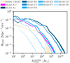 |
Fig. 2 NSC stellar mass function for the models listed in Table 1 compared to the observed NSC mass function derived from the |


3.3 Nuclear star clusters at critical mass
To understand the implications of NSCs for the formation of massive BHs, we analyze the properties of NSCs at the moment when their stellar mass is equal to the critical mass. We recall that the critical mass Mcrit (see Eq. (16)) depends on key characteristics of the NSC such as the radius, rNSC, velocity dispersion, σ, and the age, tH, of the star cluster; we used Eq. (11) to obtain the mass-weighted age of the cluster taking its star formation history into consideration. By analyzing these properties at the moment of BH seed formation, we obtained insights into the conditions driving the formation of BHs.
Figures 3, 4, 5, and 6 show the typical properties of NSCs that satisfy the conditions to form a BH seed. This particularly includes their radius, velocity dispersion, the mass-weighted age, and the redshift when their mass is equal to the critical mass; all are shown as a function of the stellar mass of the NSC. In Fig. 3, we focus on models A2, A3, and A4, which share the same parameter Ares = 10−1 and consider a minimum NSC mass of 103 M⊙. The models, however, employ different mass–radius relations for the NSCs, considering values of ϵr between 0.1 and 1. Model A1 is not shown as in this case the radii are too large for the NSCs to reach the critical mass. For model A2 with ϵr = 0.5, some NSCs reach the critical mass, with their masses ranging between 103 M⊙ and ~2 X 10³ M⊙. The radii of the NSCs are on the somewhat lower end of the general mass-radius relation (Eq. (2)), as the stellar masses of the NSCs are typically below 106 M⊙ . The radii of the clusters considered here are slightly enhanced, as the mass-radius relation from Eq. (2) considers the dynamical mass including the gas, leading to the presence of some scatter in the relation between NSC radius and stellar mass.
The number of NSCs for which the NSC mass becomes equal to the critical mass increases significantly in model A3 where ϵr = 0.2, as the critical mass decreases strongly with decreasing radius. This becomes even more pronounced for model A4 with ϵr = 0.1. For NSCs with masses above 105 M⊙, the typical radii are in the range 0.1–1 pc, and shift toward ~0.1 pc for even lower-mass clusters. The velocity dispersions are around 10 km/s for low-mass clusters and more than around 100 km/s for intermediate-mass ones, again with spread depending on the presence of gas in the system. The spread is enhanced in models A3 and A4 as the decrease in the general mass–radius relation implies that even NSCs with larger amounts of gas (and thereby radii enhanced by the presence of gas) can still become unstable to collisions. The stellar mass of the NSCs forms a power law with the velocity dispersion of the NSCs as  though with a decrease in the overall spread as the stellar mass increases. In terms of the ages of the NSCs, there is also a significant variation; for model A2 most of the NSCs that form BHs are older than 6 Gyr, while in models A3 and A4 there is a significant spread over the ages ranging from systems with ages of 7.5 Gyr up to even relatively young but more compact NSCs. As a result the BH seeds form over a range of redshift, between redshift ~4 and redshift 0. We note that there is a wide spread in formation redshifts for the lower-mass NSCs, while the more massive ones form around redshift 0.
In Fig. 4, we show models A7 and A8 with parameters ϵr = 0.2 and 0.1, but a mass threshold of 104 M⊙. We do not show models A5 and A6 because the critical mass is not reached due to their radii. The behavior is overall similar to Fig. 3; the main difference is a somewhat larger spread in the correlations at the threshold mass ~104 M⊙ but otherwise the same type of behavior and relations. The increase in the threshold effectively also represents a delay for the formation of the first BH seeds, as larger structures first have to form for them to potentially come into place.
The models shown in Figs. 5–6, D3, D4, D7, and D8, correspond to a diminished rate of gas transference to the reservoir (Ares = 10−2) in comparison with models A. This results in less gaseous material available to form stars in the nuclear region leading to lower SFRs, leading to a delay in the formation of massive NSCs. This is clearly visible in model D4 where the mass threshold is equals to 103 M⊙, and the efficiency ϵr is 0.1. A direct comparison with model A4, which shares the same parameters except for the enhanced value of Ares shows that in A4 the formation of the seeds starts at earlier times (ɀ ~ 4) when the value of Ares is higher.
An important difference is model D2 do not form any BH seed as model A2, this is caused due to the relative low gas transfer, which impacts directly in the radius of the NSCs and avoid the formation of BHs. Instead, models D3 and D4, with ϵr equals to 0.2 and 0.1, form seeds for a variety of ages ranging from very young systems and up to ages of ~7.5 Gyr. The more massive NSCs are typically older and will form more massive BHs, though at a correspondingly lower redshift. For example, heavy seeds with masses on the order of 105 M⊙ start to form at redshift ɀ ~ 0.2, while the formation of light-medium seeds starts at ɀ ~ 2.4 in model D4.
Increasing the value of Mthreshold to 104 M⊙ just delay the formation of seeds in models D7 and D8, similar to what was seen for models A7 and A8. Again model D8 with ϵr = 0.1 starts to form seeds at earlier times than model D7 (ϵr = 0.2) due to the more compact radius. The behavior is very similar to the behavior already noted above. The most massive seeds are formed in older systems and at low redshifts as the most massive NSCs form at those redshift. The first seeds are formed in model D8 at ɀ ~ 1.8, with masses on the order of 5 x 10³ M⊙, while the formation of seeds in NSCs with stellar masses up to 105 M⊙ results in seeds larger than 5 x 10⁴ M⊙ from ɀ ~ 0.75. Model D7 starts forming the lightest seeds at ɀ ~ 0.7 and the most massive seeds (~104 M⊙) at ɀ = 0.
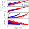 |
Fig. 3 Radius of the NSC (rNSC) multiplied by the respective efficiency (ϵr), velocity dispersion (σ) at rNSC, age of the system (tH), and the redshift as a function of the stellar mass of the NSC for models A2 (rose dots), A3 (blue dots), and A4 (red dots). Mthreshold = 103 M⊙ and Ares = 10−1 for all the models. The values of ϵr are 0.5, 0.2, and 0.1 for models A2, A3, and A4, respectively, as listed in Table 1. These properties are extracted at the moment at which the conditions to form a BH seed are fulfilled ( |


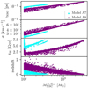 |
Fig. 4 Same as Fig. 3 but for models A7 (cyan dots) and A8 (purple dots), with Mthreshold = 104 M⊙ and ϵr = 0.2, and 0.1, respectively, as listed in Table 1. Models A5 and A6 do not form any BH seed as the conditions for seeding ( |


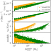 |
Fig. 5 Same as Fig. 3 but for models D3 (orange dots) and D4 (green dots), for Mthreshold = 103 M⊙ 103 M⊙ and Ares = 10−2. The values of ϵr for each model are 0.5, 0.2, and 0.1, respectively, as listed in Table 1. Models D1 and D2 do not form any BH seed as the conditions for seeding ( |


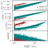 |
Fig. 6 Same as Fig. 3 but for models D7 (brown dots) and D4 (teal dots), with Mthreshold = 104 M⊙ and ϵr = 0.5 and 0.1, respectively, as listed in Table 1. Models D5 and D6 do not form any BH seed as the conditions for seeding ( |


3.4 Black hole mass function
In this subsection we present the black hole mass function (BHMF) obtained via the different models through GALACTICUS for redshift ɀ = 0 hosted in galaxies with stellar masses above 106 M⊙ and coexisting with NSC with stellar masses higher than 103 M⊙ . Thereby, we compared the model predictions with the BHMF from observations of the Local Universe estimated by Vika et al. (2009). This particularly allowed us to study the impact of Ares, ϵr, and Mthreshold on the population at ɀ = 0 through the proposed scenario previously introduced in Sect. 2.2 and implemented in GALACTICUS as described in Sect. 2.2.2.
In Fig. 7, we provide the BHMF (Φ•) for all the models listed in Table 2, except for the models that do not form any seeds (due to the NSCs not reaching the critical mass). In general, models A2, B2, C2, E2, F2, G2, and H2, with parameters Mthreshold = 103 M⊙ and ϵr = 0.5 have a BHMF that starts with an initial increase from Φ• ~ 10−2 [Mpc−3 dex−1] at MBH = 105 M⊙ to Φ• ~ 2 X 10⁻¹ [Mpc−3 dex−1] at MBH = 3 X 10⁶ M⊙, presumably as the BHs rapidly grow in mass and do not stay in that mass range for a significant amount of time. At higher masses, all the models (including models with ϵr = 0.2, 0.1, and Mthreshold = 104 M⊙) show an increase in the population of SMBHs until they reach a peak on the population at masses on the order 106 M⊙ where Φ• ~ 5 [Mpc−1 dex−1]. From this peak toward higher masses, Φ• decreases monotonically until reaching the maximum BH mass that is still realized in one of the DM halos modeled via GALACTICUS, which in general is up to a few times 109 M⊙, with Φ• oscillating between ~10−5 and 10−4 [Mpc−3 dex−1].
In all of our models, it is possible to distinguish differences in the BHMF when comparing different values of ϵr at a fixed Ares. In models E, Φ• is enhanced by a factor of ~10 in model E2 compared to E3 for SMBH masses in the range 105−107 M⊙, while at higher masses the models give comparable predictions for the mass function. Such differences at lower masses are not seen in models with fast gas transfer (high Ares), where models with ϵr = 0.1 and 0.2 are essentially indistinguishable.
The decrease in Φ• for SMBHs with masses higher than >107 M⊙ indicates that such massive objects are less frequent compared to the total population predicted in our models. Models with ϵr = 0.1 (A4, A8, B4, B8, C4, C8, E4, F4, G4, and H4) include the formation of SMBHs with masses up to a few times 109 M⊙ in some of the halos. Combining this information with Figs. 4–6, and Table 2, we note that these models form heavier seeds than models A2, A3, and D3, which form at most medium seeds at earlier times, allowing those seeds to accrete more material from their environment.
The BHMF from Vika et al. (2009) is comparable with the high-end mass in almost all our models for BH masses above 108 M⊙. Particularly, at below masses of 108 M⊙, the models tend to overpredict the observed population by at least a factor of 10. The overestimation is about 102 times in masses on the order of 106−107 M⊙, where the uncertainties of the BHMF becomes larger due to the observational limits.
The underestimation at higher masses does not represent a problem, as here we considered only one seeding mechanism, and other mechanisms could still change the overall picture, including even the possibility of mergers of some of the SMBHs formed here with other seeds. The comparison also shows that quite a significant number of BHs seeds can be formed in this manner, providing a relevant contribution to the general population.
For a detailed quantitative analysis of the over- or underestimation of the BHMF in our models, we kindly refer readers to our Appendix B.
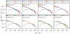 |
Fig. 7 Comparison between the BHMF determined by Vika et al. (2009, gray dots) with our SAMs at ɀ = 0 for galaxies with stellar masses higher than 106 M⊙ that host NSCs with stellar masses above 103 M⊙. The gray dots include the ±1σ error bars, while the thickness of our lines denotes the ±1σ error for our SAMs, estimated as |

Range of BH masses formed in our SAMs.
Values of the best-fit parameters c1 and c2 .
3.5 Nuclear star clusters, supermassive black holes, and host galaxies
We explored the scaling relations between the global properties of the NSCs and their host galaxies. We included in our analysis the masses of NSCs and SMBHs coexisting in the observed galactic nuclei from Seth et al. (2008a), Graham & Spitler (2009), Neumayer & Walcher (2012), Georgiev et al. (2016), and Nguyen et al. (2018). The resulting sample contains early (late)-type galaxies and stripped galaxy nuclei. We removed the ultra-compact dwarfs for which information about the stellar mass of the galaxy is not available.
We made a power-law fit for the correlation in the observed sample consideration a relation between  and
and  of the form
 (22)
(22)
where MBH is the mass of the central SMBH,  is the stellar mass of the NSC,
  is the stellar mass of the host galaxy and c1 and c2 are the free coefficients to fit.
In the 2D probability density function (PDF) corresponding to the observed sample, the ratio MBH/MNSC for galaxies of low stellar masses is dominated by the mass of the NSC, and dominated by the SMBH at the high end of galaxy stellar masses. Combining this figure with the results of the best fits given in Table 3, we see an interesting trend: as ϵr decreases, the slope of the fit approaches the slope of the observed fit, suggesting that as ϵr decreases, NSCs form more massive seeds at early times, which allows them to reach higher final masses. In Fig. 8, we show the  correlation predicted by GALACTICUS for galaxies with stellar masses higher than 106 M⊙ hosting NSCs and SMBHs with masses higher than 103 M⊙ and 105 M⊙, respectively.
We find that NSCs and SMBHs coexist in models A2, A3, A4, A7, and A8. We included the contour lines of the 2D PDF as dashed lines and the thick solid line corresponds to the 1σ of the 2D PDF. The results of the different fits are included as dashed lines, where the shadow areas indicate the 1σ error of the fit slope and intercept coefficient. We encourage readers to refer to Appendix C for further details on the PDF.
Model A2 shows an overlap with the observed correlation for galaxies with stellar masses from ∼108 M⊙ to ∼1011 M⊙ with a  ranging from 10−1 to 102. Although there is an overlap between our predictions and the observations, GALACTICUS shows a big spread in the
  ratio for galaxies with stellar masses below 1010 M⊙. In particular, almost all the galaxies are contained outside the overlap with the observations at ~107 M⊙ hosting a SMBH with
  . Furthermore, GALACTICUS predicts the existence of a population of galaxies with masses on the order of 1011 M⊙, which overlaps well with observations. This population corresponds to galaxies that recently formed a BH seed under the proposed scenario in NSCs with stellar masses on the order of ∼109 M⊙ to ∼1010 M⊙, forming seeds with similar masses.
Models A3 and A7 (ϵr = 0.2 and Mthreshold = 103,104 M⊙, respectively) predominantly include galaxies with stellar masses on the order of 108−1011 M⊙, with  , thus providing a significant overlap between the models and observations at the contour lines. Models A4 and A8 (ϵr = 0.1 and Mthreshold = 103 and 104 M⊙, respectively), on the other hand, show the best overlap around
  , and the values of
  are less spread in comparison to the models A3 and A7. Furthermore, the distribution of the galaxies is moving toward the observed sample contours, but with a different slope as listed in Table 3.
We previously found that the models labeled with D provide better predictions for the maximum stellar masses of NSCs, as demonstrated by the comparison of predicted and observed NSC mass function in Fig. 2. In Fig. 8, we observe a similar trend as models A. It is clear that models D4 and D8, with Mthreshold = 103 M⊙ and Mthreshold = 104 M⊙, respectively, and ϵr = 0.1, show an overlap from  to
to  with observations, quite similar to models A4 and A8. The values of
  range from 10−2 to ∼102, meaning that NSCs and SMBHs have similar masses or at most there is a mass difference by two orders of magnitude. The impact of ϵr is reflected in the value of c1 and c2 given in the best fit in Table 3. As the value of ϵr decreases, the values of the free parameters fitted to our models approach the values of the observed correlation.
Figure 9 shows the same as Fig. 1, but we made a distinction between galaxies with NSCs hosting (or not hosting) SMBHs. In model G4, all the galaxies that host a NSC with stellar masses higher than 104 M⊙ host a SMBH in their center. For models A4 and A8 where ϵr = 0.1, 58% and 54% of the galaxies host both types of objects (NSCs and SMBHs, respectively). For models with larger values of ϵr, the fraction drops as the formation of seeds becomes less efficient. In consequence, the number of galaxies hosting a SMBH decreases for models A2, A3, and A7, where the SMBH occupation fraction is 1%, 20%, and 12%, respectively. For models D, on the other hand, we find SMBH occupation fractions of 90% and 88%, respectively, for models D4 and D8, and 2%, 52%, and 35% for models D3 and D7.
We find that there is a scaling relation between the stellar mass of the NSC and the stellar mass of the galaxy in all our models as well as in the observed population. In our models, galaxies with stellar masses between 109 M⊙ and 1011 M⊙ show a scatter in the stellar mass of the NSC in galaxies hosting a SMBH. A possible explanation for this is the fact of the SMBH accreting material from the NSC gas reservoir, removing a fraction of the available gas for star formation in the NSC. This loss of gas directly affects the SFR of the NSC as  , suggesting that BH suppress the in situ star formation in NSCs.
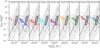 |
Fig. 8
|


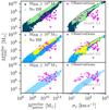 |
Fig. 9 Same as Fig. 1 but for models with BH formation (A4, D4, and G4). We distinguish model galaxies that host (or not) a SMBH in their center. Triangles indicate upper limits for the stellar mass estimation of the NSCs. |
4 Discussion and conclusions
In this work, we employed the SAM GALACTICUS developed by Benson (2012) to explore the seeding of SMBHs via collisions in NSCs. We used the framework proposed by Escala (2021), where SMBHs are formed from (partially) failed NSCs with average collision timescales shorter than the age of the system, thus implying the efficient formation of a central massive object via runaway collisions. In particular, we employed the concept of the critical mass scale, for which the average timescale for collisions within the NSC (of a given radius) is equal to the age of the cluster. This was introduced by Vergara et al. (2023) to numerically test this framework (with successful results), and they later extended its validity to a range of stellar systems (GCs and ultra-compact dwarf galaxies, in addition to NSCs; Vergara et al. 2024). The formation of NSCs themselves is modeled here via the in situ mechanism, which is adequate for the more massive galaxy population and thus for the formation of SMBHs in more massive galaxies (Antonini & Perets 2012; Antonini et al. 2015).
Within this framework, we find that the formation of NSCs and their mass function is regulated through the efficiency parameter, which describes the gas mass transfer to the center of the galaxy. Here it is taken to be proportional to the global SFR. The mass function we obtain in our models is comparable in terms of shape with the NSC mass function constructed using the  relation and the fitted galaxy stellar mass function derived by Baldry et al. (2012). There is also considerable overlap in the observed scaling relations between the NSC mass and the stellar mass of the galaxy. The comparison, however, suggests that in real galaxies there is not one fixed value for the efficiency to transport gas into the center; the efficiency may depend on the galaxy and its environment. The maximum observed stellar masses observed are on the order of 109 M⊙. The efficiency parameters we employed to find agreement with observations are consistent with those reported by Antonini et al. (2015) and used in their SAM.
Although there is an agreement for NSC masses of about ∼108 M⊙, our models in general overestimate the NSC mass function by a factor of 10. As mentioned in Sect. 3.2, this is not an issue as in low-mass NSCs the observed NSC mass function is a lower limit. We find that the size of the population of NSCs in the lower-mass regime depends strongly on the value of Ares.
Although we cannot make a direct comparison with the observed NSC, our estimation is reliable for masses above 105 M⊙ ; however, due to the limit of observations, our models in general overestimate the population of NSCs. We also remark that deriving a NSC mass function from observations is often difficult at the low end of NSC masses due to the low resolution, which is insufficient to study remote and distant NSCs in detail (Côté et al. 2006). Additionally, there is an ongoing issue with the criteria for defining what constitutes a NSC; the definition of NSCs could be biased due ambiguity in the classification, that is, some clusters might be classified as NSCs according to one definition and not according to another. Furthermore, NSCs can be difficult to distinguish from the central bulges of galaxies, where the background light of the most luminous bulges plays an important role in galaxies with a Hubble type t ≥ 3.5 (Georgiev & Böker 2014). Other issues affect the study of elliptical and lenticular galaxies, where the stellar density gradient can be smooth and delineating where the bulge ends and the NSC begins is challenging as the galactic nuclei do not show a clear discontinuity, especially in galaxies where the NSC and bulge have a similar brightness profile (Carollo et al. 1997; Côté et al. 2006; Böker 2010; Neumayer et al. 2020).
Our overestimation of the population may indicate that the in situ star formation scenario is sufficient to explain the population of the most massive NSCs but is not the main mechanism in the low-mass regime. This would suggest that the invocation of other formation mechanisms, such as the migration of GCs (e.g., Tremaine et al. 1975; Capuzzo-Dolcetta 1993), is also required and that the value of Ares is not constant for all galaxies but instead depends on environmental factors. Previous studies have suggested a correlation between the morphological type of the host galaxy and the formation scenario of the NSC: the GC infall scenario is related to early-type galaxies (Tremaine et al. 1975; Capuzzo-Dolcetta 1993), while in massive late-type galaxies the in situ formation dominates the growth of the NSC (Pinna et al. 2021; Hannah et al. 2021). In our models we assume that the gas transfer to the nuclear reservoir is related to the star formation in the spheroidal component of the galaxies. This is consistent with galaxies that typically have abundant gas, which provides a rich gas reservoir for in situ star formation within the nucleus of the galaxies. As our model does not account for the population of NSCs formed in bulge-less galaxies or those without a significant spheroidal component, where dynamical processes are the main formation mechanism, we are missing part of the population of NSCs formed via the cluster infall scenario. This scenario is particularly predominant in early-type galaxies, where NSCs are more likely to form through the accumulation and merging of preexisting GCs that migrate to the center over time, as explored by Capuzzo-Dolcetta (1993) in a triaxial galaxy model, via N- body simulations (Milosavljević 2004), and more recently via self-consistent numerical simulations (Bekki 2010).
For the formation of massive BHs via collisions, a crucial aspect is the mass–radius correlation of NSCs. We did not explore this correlation from first principles but rather adopted the observed correlation from Neumayer et al. (2020) and varied it via a parameter ϵr, taking into consideration the range of the observed radii as well as the possibility of evolution over cosmic time. As expected, more compact NSCs result in an earlier formation of more massive BH seeds due to them being more favorable for stellar collisions and thus increasing the probability of forming a seed, which directly affects the fraction of galaxies that host both NSCs and SMBHs. Models with ϵr = 0.1 are able to form more massive seeds at earlier times, at redshifts of 3 or 4. As mentioned in Sect. 2.2.1, this is consistent with the study of Banerjee & Kroupa (2017), who show that the effective radius of massive star clusters can change by more than a factor of 10. Our models show a significant correlation between the NSC mass and the stellar mass (and the velocity dispersion) of the host galaxy, which follows a power-law distribution. This correlation also holds when varying the efficiency parameter for the mass transport to the center of the galaxy, and the correlation is independent of the potential presence of a SMBH. The spread in the stellar mass of the NSCs at a fixed galaxy stellar mass, however, increases when the NSCs host a SMBH. As mentioned, less massive NSCs could be due to a decrease in the SFR as the BH seed accretes gaseous material from the nuclear reservoir.
In general, all our models are able to produce BH seeds, except those with ϵr = 1, and only a few seeds form in models with ϵr = 0.5. This may suggest that in the observed population the mechanism also operates preferably in the more compact part of the population, or possibly also at early stages when the NSCs were still more compact. Overall, the models are able to produce a range of BHs from light seeds (∼102 M⊙) to heavy seeds (∼105 M⊙). The formation of the most massive seeds (∼105 M⊙) is independent of the mass threshold we employed for the NSCs but only happens in models where ϵr = 0.1. Furthermore, those seeds are formed in systems with ages of ≳ 4 Gyrs and velocity dispersions higher than 70 km s−1 . The formation of these massive seeds, however, happens relatively late, that is, at redshifts ɀ ∼ 0.35, within the halos modeled here. We cannot rule out the possibility that this also happens early in some cases, and in this respect it might be important to study the halo merger history of the first quasars that formed around ɀ ∼ 6 to obtain more insight into their specific histories and to understand whether this channel might be contributing there. In this context, the presence of gas within the NSCs might be even more relevant, and it could be important to include the extension of the critical mass concept in the presence of gas, as recently proposed by Vergara et al. (2024). In addition, it is clear that other seeding scenarios may also contribute to the general population, and the interaction between different seeding mechanisms (i.e., due to mergers) needs to be explored. This includes, for example, seeding via direct collapse (Bromm & Loeb 2003; Koushiappas et al. 2004; Wise et al. 2008; Latif et al. 2013, 2022) as well as mixed scenarios that take the interaction of collisions and accretion into account (Boekholt et al. 2018; Chon & Omukai 2020; Schleicher et al. 2022, 2023; Reinoso et al. 2023).
Our models successfully reproduce the shape of the observed mass functions of NSCs and SMBHs, showing particularly strong matches within the mass range relevant to SMBH formation. However, they overpredict the NSC and BH mass functions at lower masses, likely due to an excess (by a factor of ∼10) in the number of galaxies predicted by GALACTICUS compared to the Baldry et al. (2012) sample.
Despite this discrepancy, our results demonstrate that the proposed scenario effectively forms BH seeds capable of growing to masses of up to 109 M⊙. A logical next step is to enhance the statistical robustness of our predictions. Unfortunately, rescaling the stellar mass function is not straightforward. One potential approach is to employ the Markov chain Monte Carlo (MCMC) functionality built into GALACTICUS. While MCMC can improve statistical predictions, it requires a significant computational investment to achieve reliable results.
The predicted scaling relations also overlap considerably with observed data. For BH masses of around 107 M⊙, our model overpredicts the observed population (constructed from the Vika et al. 2009 sample) by roughly a factor of 10, while at higher masses we tend to underpredict the observed population. This of course may change when additional BH formation mechanisms are considered, and some of the BH seeds predicted by our model may also merge with seeds produced via different channels (Sassano et al. 2021; Trinca et al. 2022).
Nonetheless, the comparison shows that the collision-based channel may contribute in a relevant way to the overall population. This could include a related but different mechanism, for example the formation of massive BHs in dark cores that are formed in the center of NSCs (e.g., Davies et al. 2011; Lupi et al. 2014; Kroupa et al. 2020; Gaete et al. 2024). We expect more light to be shed on the seeds of SMBHs with upcoming observations from the JWST and the Extremely Large Telescope (ELT)4 together with the emission of gravitational waves detected by current interferometers, such as the Laser Interferometer Gravitational-Wave Observatory (LIGO)5/Virgo6/ Kamioka Gravitational Wave Detector (KAGRA)7 collaboration (Abbott et al. 2024), and in the future with the Laser Interferometer Space Antenna (LISA) (Amaro-Seoane et al. 2017) and the Einstein Telescope8 (Punturo et al. 2010), both in the local and the high-redshift Universe.
Acknowledgements
We gratefully acknowledge support by the ANID BASAL project FB21003, Fondecyt Regular (project code 1201280) and ANID-Quimal 220002. DRGS thanks for funding via the Alexander von Humboldt – Foundation, Bonn, Germany. MCV acknowledges funding through ANID (Doctor-ado acuerdo bilateral DAAD/62210038) and DAAD (funding program number 57600326). ML would also like to express his gratitude to Dr. Nadine Neumayer for her valuable discussions and comments during his visit to MPIA, Heidelberg, and to Dr. Enrico Barausse for his insightful feedback during my time at SISSA, Trieste.
Appendix A Mass resolution and convergence tests
We checked the convergence of the GALACTICUS output running the same models listed in Table 1 by changing the mass resolution. In Fig. A.1, the top panel shows the NSC mass function for mass resolutions on the order of 105, 106, 107, 108, and 109 M⊙. We note that mass functions show a different shape in lower resolutions (that means solving DM halos with masses equal or lager than the resolution).
Although the mass function is converged for NSC with stellar masses in the range 107–1010 M⊙, it starts to converge in the low regime in resolutions higher than ~107 M⊙. As shown in the bottom panel of the Fig. A.1, the relative error of ΦNSC (relative to model A1 with a resolution of 4.86 × 10⁵ M⊙) is less than Δ log ΦNSC < 0.5, and decreases as the mass resolution increases.
We also check the convergence for the BH mass function. As model Al does not form nay seed, we show the results of the convergence test for model A4 in Figs. A.1, A.2. We found that the convergence of the BH mass function begins in high mass resolutions, such as 4.86 × 10⁷, ×106, and ×105 M⊙. Because of the agreement in the convergence of the NSC and BH mass functions we adopt a resolution equals to 4.86 × 10⁵ M⊙.
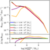 |
Fig. A.1 NSC mass function for the different mass resolutions specified in the legend. The error is relative to model A4, which has a higher mass resolution (4.86 × 10⁵ M⊙ and color blue). |
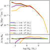 |
Fig. A.2 BH mass function for the different mass resolutions specified in the legend. The error is relative to model A4, which has a higher higher mass resolution (4.86 × 10⁵ M⊙). |
Appendix B Galaxy and black hole mass function deviations
We compared the galaxy mass function of Baldry et al. (2012) with the mass function of galaxies hosting a NSC with stellar mass over 103 M⊙ predicted by GALACTICUS to quantify how far our models deviate from observations. We defined  at each bin. Afterward, we computed the average and the maximum (minimum) value of q per model.
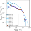 |
Fig. B.1 Galaxy stellar mass function at ɀ = 0 for eight models run in GALACTICUS (solid lines) and the galaxy stellar mass function of (Baldry et al. 2012, orange dots). |
From Fig. B.1 we find (on average) an overestimation of the observed galaxy stellar mass function on the order of 0.5–0.6 ± 0.3 dex, except for model HI, which shows the lowest (averaged) overestimation but larger standard deviation (0.33 ± 0.5 dex). It is important to note that the major discrepancy is observed at  M⊙. We stress that the observed mass function should be considered as a lower limit due to the GAMA survey limitations explained in Sect. 3.2. As a result, our calculation of the deviation in this range represents an upper limit, meaning that any future refinements to the models will only improve the agreement. For the BHMF we list the averages and maximum (minimum) values in Table B.1.
Deviations for various models across different BH mass ranges.
Appendix C Probability density function
For the different fits made to the datasets we estimated the PDF using the kernel density estimation nonparametric technique using the SCIPY package available for PYTHON. We encourage readers to review the mathematical formulation in Scott (2015).
We fit the distribution of the stellar mass of the galaxy and the ratio between the MBH and the  assuming a Gaussian kernel. An important parameter to choose when the PDF is estimated is the bandwidth. In Figs. C.1 and C.2, we show the PDF as a function of the bandwidth for the observed distribution. In both cases we chose the value of 0.5 as it recovers the shape of the original distribution and provides a smooth fit to the observed data.
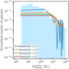 |
Fig. C.1 Normalized number of galaxies as a function of their stellar mass (y-axis). We plot the different values of the bandwidth parameter that regulates the fit using the kernel density estimation technique. |
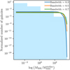 |
Fig. C.2 Same as Fig. C.1 but showing the normalized distribution of galaxies as a function of the ratio between the mass of the BH and the stellar mass of the NSC. |
Appendix D Observed properties of galaxies hosting NSCs and SMBHs
In Table D.1 we provide a compilation of the properties of the galaxies hosting NSCs and SMBHs based on the sample of Neumayer et al. (2020), but additionally adding the velocity dispersion from the host galaxy employing literature data.
Properties of galaxies hosting NSCs and SMBHs.
References
- Abbott, R., Abbott, T. D., Acernese, F., et al. 2024, Phys. Rev. D, 109, 022001 [NASA ADS] [CrossRef] [Google Scholar]
- Agarwal, M., & Milosavljevic, M. 2011, ApJ, 729, 35 [NASA ADS] [CrossRef] [Google Scholar]
- Amaro-Seoane, P., Audley, H., Babak, S., et al. 2017, arXiv e-prints [arXiv:1702.00786] [Google Scholar]
- Antonini, F. 2013, ApJ, 763, 62 [Google Scholar]
- Antonini, F., & Perets, H. B. 2012, ApJ, 757, 27 [NASA ADS] [CrossRef] [Google Scholar]
- Antonini, F., Barausse, E., & Silk, J. 2015, ApJ, 812, 72 [Google Scholar]
- Bañados, E., Venemans, B. P., Decarli, R., et al. 2016, ApJS, 227, 11 [Google Scholar]
- Balcells, M., Graham, A. W., Domínguez-Palmero, L., & Peletier, R. F. 2003, ApJ, 582, L79 [Google Scholar]
- Baldry, I. K., Driver, S. P., Loveday, J., et al. 2012, MNRAS, 421, 621 [NASA ADS] [Google Scholar]
- Balick, B., & Brown, R. L. 1974, ApJ, 194, 265 [NASA ADS] [CrossRef] [Google Scholar]
- Banerjee, S., & Kroupa, P. 2017, A&A, 597, A28 [NASA ADS] [CrossRef] [EDP Sciences] [Google Scholar]
- Barth, A. J., Ho, L. C., & Sargent, W. L. W. 2002, AJ, 124, 2607 [NASA ADS] [CrossRef] [Google Scholar]
- Barth, A. J., Strigari, L. E., Bentz, M. C., Greene, J. E., & Ho, L. C. 2009, ApJ, 690, 1031 [NASA ADS] [CrossRef] [Google Scholar]
- Becklin, E. E., & Neugebauer, G. 1968, ApJ, 151, 145 [Google Scholar]
- Begelman, M. C., & Rees, M. J. 1978, MNRAS, 185, 847 [NASA ADS] [CrossRef] [Google Scholar]
- Bekki, K. 2007, PASA, 24, 77 [Google Scholar]
- Bekki, K. 2010, MNRAS, 401, 2753 [NASA ADS] [CrossRef] [Google Scholar]
- Bekki, K., Couch, W. J., & Shioya, Y. 2006, ApJ, 642, L133 [Google Scholar]
- Bender, R., Kormendy, J., Bower, G., et al. 2005, ApJ, 631, 280 [NASA ADS] [CrossRef] [Google Scholar]
- Benson, A. J. 2012, New A, 17, 175 [NASA ADS] [CrossRef] [Google Scholar]
- Benson, A. J. 2017, MNRAS, 467, 3454 [NASA ADS] [CrossRef] [Google Scholar]
- Benson, A. J., & Bower, R. 2010, MNRAS, 405, 1573 [NASA ADS] [Google Scholar]
- Benson, A. J., Pearce, F. R., Frenk, C. S., Baugh, C. M., & Jenkins, A. 2001, MNRAS, 320, 261 [NASA ADS] [CrossRef] [Google Scholar]
- Binney, J., & Tremaine, S. 2008, Galactic Dynamics, 2nd edn. (Princeton University Press) [Google Scholar]
- Bland-Hawthorn, J., & Gerhard, O. 2016, ARA&A, 54, 529 [Google Scholar]
- Boeker, T., van der Marel, R. P., Gerssen, J., et al. 2003, SPIE Conf. Ser., 4834, 57 [NASA ADS] [Google Scholar]
- Boekholt, T. C. N., Schleicher, D. R. G., Fellhauer, M., et al. 2018, MNRAS, 476, 366 [Google Scholar]
- Böker, T. 2010, in Star Clusters: Basic Galactic Building Blocks Throughout Time and Space, 266, eds. R. de Grijs, & J. R. D. Lépine, 58 [Google Scholar]
- Böker, T., van der Marel, R. P., & Vacca, W. D. 1999, AJ, 118, 831 [CrossRef] [Google Scholar]
- Bower, G. A., Green, R. F., Danks, A., et al. 1998, ApJ, 492, L111 [Google Scholar]
- Bower, G. A., Green, R. F., Bender, R., et al. 2001, ApJ, 550, 75 [Google Scholar]
- Bower, R. G., Vernon, I., Goldstein, M., et al. 2010, MNRAS, 407, 2017 [NASA ADS] [CrossRef] [Google Scholar]
- Bromm, V., & Loeb, A. 2003, ApJ, 596, 34 [Google Scholar]
- Burbidge, E. M., Burbidge, G. R., & Fish, R. A. 1961, ApJ, 134, 251 [NASA ADS] [CrossRef] [Google Scholar]
- Cappellari, M., Verolme, E. K., van der Marel, R. P., et al. 2002, ApJ, 578, 787 [NASA ADS] [CrossRef] [Google Scholar]
- Cappellari, M., McDermid, R. M., Alatalo, K., et al. 2013, MNRAS, 432, 1862 [NASA ADS] [CrossRef] [Google Scholar]
- Capuzzo-Dolcetta, R. 1993, ApJ, 415, 616 [NASA ADS] [CrossRef] [Google Scholar]
- Capuzzo-Dolcetta, R., & Mastrobuono-Battisti, A. 2009, A&A, 507, 183 [NASA ADS] [CrossRef] [EDP Sciences] [Google Scholar]
- Carollo, C. M., Stiavelli, M., de Zeeuw, P. T., & Mack, J. 1997, AJ, 114, 2366 [NASA ADS] [CrossRef] [Google Scholar]
- Chon, S., & Omukai, K. 2020, MNRAS, 494, 2851 [Google Scholar]
- Cole, S., Lacey, C. G., Baugh, C. M., & Frenk, C. S. 2000, MNRAS, 319, 168 [Google Scholar]
- Côté, P., Piatek, S., Ferrarese, L., et al. 2006, ApJS, 165, 57 [Google Scholar]
- Côté, B., Silvia, D. W., O’Shea, B. W., Smith, B., & Wise, J. H. 2018, ApJ, 859, 67 [CrossRef] [Google Scholar]
- Cretton, N., & van den Bosch, F. C. 1999, ApJ, 514, 704 [NASA ADS] [CrossRef] [Google Scholar]
- Cross, N., & Driver, S. P. 2002, MNRAS, 329, 579 [NASA ADS] [CrossRef] [Google Scholar]
- Croton, D. J., Stevens, A. R. H., Tonini, C., et al. 2016, ApJS, 222, 22 [Google Scholar]
- Dametto, N., Riffel, R., Pastoriza, M., et al. 2014, MNRAS, 443, 1754 [CrossRef] [Google Scholar]
- Davies, M. B., Miller, M. C., & Bellovary, J. M. 2011, ApJ, 740, L42 [NASA ADS] [CrossRef] [Google Scholar]
- de Francesco, G., Capetti, A., & Marconi, A. 2006, A&A, 460, 439 [NASA ADS] [CrossRef] [EDP Sciences] [Google Scholar]
- den Brok, M., Seth, A. C., Barth, A. J., et al. 2015, ApJ, 809, 101 [NASA ADS] [CrossRef] [Google Scholar]
- Devereux, N., Ford, H., Tsvetanov, Z., & Jacoby, G. 2003, AJ, 125, 1226 [NASA ADS] [CrossRef] [Google Scholar]
- Di Carlo, U. N., Mapelli, M., Pasquato, M., et al. 2021, MNRAS, 507, 5132 [NASA ADS] [CrossRef] [Google Scholar]
- Ding, X., Silverman, J., Treu, T., et al. 2020, ApJ, 888, 37 [NASA ADS] [CrossRef] [Google Scholar]
- Ebisuzaki, T. 2003, in Astrophysical Supercomputing using Particle Simulations, 208, eds. J. Makino, & P. Hut, 157 [Google Scholar]
- Edgar, R. 2004, New Astron. Rev., 48, 843 [CrossRef] [Google Scholar]
- Emsellem, E., & van de Ven, G. 2008, ApJ, 674, 653 [CrossRef] [Google Scholar]
- Emsellem, E., Dejonghe, H., & Bacon, R. 1999, MNRAS, 303, 495 [CrossRef] [Google Scholar]
- Escala, A. 2021, ApJ, 908, 57 [NASA ADS] [CrossRef] [Google Scholar]
- Faber, S. M., & Jackson, R. E. 1976, ApJ, 204, 668 [Google Scholar]
- Fan, X., Bañados, E., & Simcoe, R. A. 2023, ARA&A, 61, 373 [NASA ADS] [CrossRef] [Google Scholar]
- Ferrara, A., Salvadori, S., Yue, B., & Schleicher, D. 2014, MNRAS, 443, 2410 [NASA ADS] [CrossRef] [Google Scholar]
- Ferrarese, L., & Merritt, D. 2000, ApJ, 539, L9 [Google Scholar]
- Ferrarese, L., Ford, H. C., & Jaffe, W. 1996, ApJ, 470, 444 [NASA ADS] [CrossRef] [Google Scholar]
- Ferrarese, L., Côté, P., Dalla Bontà, E., et al. 2006, ApJ, 644, L21 [Google Scholar]
- Filippenko, A. V., & Ho, L. C. 2003, ApJ, 588, L13 [NASA ADS] [CrossRef] [Google Scholar]
- Freitag, M., Gürkan, M. A., & Rasio, F. A. 2006a, MNRAS, 368, 141 [NASA ADS] [Google Scholar]
- Freitag, M., Rasio, F. A., & Baumgardt, H. 2006b, MNRAS, 368, 121 [NASA ADS] [CrossRef] [Google Scholar]
- Gaete, B., Schleicher, D. R. G., Lupi, A., et al. 2024, A&A, 690, A378 [NASA ADS] [CrossRef] [EDP Sciences] [Google Scholar]
- Gebhardt, K., Lauer, T. R., Kormendy, J., et al. 2001, AJ, 122, 2469 [CrossRef] [Google Scholar]
- Gebhardt, K., Richstone, D., Tremaine, S., et al. 2003, ApJ, 583, 92 [Google Scholar]
- Gebhardt, K., Adams, J., Richstone, D., et al. 2011, ApJ, 729, 119 [Google Scholar]
- Geha, M., Guhathakurta, P., & van der Marel, R. P. 2002, AJ, 124, 3073 [CrossRef] [Google Scholar]
- Geller, M. J., Diaferio, A., Kurtz, M. J., Dell’Antonio, I. P., & Fabricant, D. G. 2012, AJ, 143, 102 [NASA ADS] [CrossRef] [Google Scholar]
- Genzel, R., Eisenhauer, F., & Gillessen, S. 2010, Rev. Mod. Phys., 82, 3121 [Google Scholar]
- Georgiev, I. Y., & Böker, T. 2014, MNRAS, 441, 3570 [Google Scholar]
- Georgiev, I. Y., Böker, T., Leigh, N., Lützgendorf, N., & Neumayer, N. 2016, MNRAS, 457, 2122 [Google Scholar]
- Glebbeek, E., Gaburov, E., de Mink, S. E., Pols, O. R., & Portegies Zwart, S. F. 2009, A&A, 497, 255 [NASA ADS] [CrossRef] [EDP Sciences] [Google Scholar]
- González Delgado, R. M., Pérez, E., Cid Fernandes, R., & Schmitt, H. 2008, AJ, 135, 747 [CrossRef] [Google Scholar]
- Graham, A. W., & Spitler, L. R. 2009, MNRAS, 397, 2148 [NASA ADS] [CrossRef] [Google Scholar]
- Graham, A. W., & Soria, R. 2019, MNRAS, 484, 794 [Google Scholar]
- Granato, G. L., De Zotti, G., Silva, L., Bressan, A., & Danese, L. 2004, ApJ, 600, 580 [Google Scholar]
- Gray, E. I., Read, J. I., Taylor, E., et al. 2024, arXiv e-prints [arXiv:2405.19286] [Google Scholar]
- Gültekin, K., Richstone, D. O., Gebhardt, K., et al. 2009a, ApJ, 695, 1577 [CrossRef] [Google Scholar]
- Gültekin, K., Richstone, D. O., Gebhardt, K., et al. 2009b, ApJ, 698, 198 [Google Scholar]
- Gürkan, M. A., Freitag, M., & Rasio, F. A. 2004, ApJ, 604, 632 [NASA ADS] [CrossRef] [Google Scholar]
- Haiman, Z. 2004, ApJ, 613, 36 [Google Scholar]
- Haiman, Z., Ciotti, L., & Ostriker, J. P. 2004, ApJ, 606, 763 [NASA ADS] [CrossRef] [Google Scholar]
- Hannah, C. H., Seth, A. C., Nguyen, D. D., et al. 2021, AJ, 162, 281 [NASA ADS] [CrossRef] [Google Scholar]
- Henriques, B. M. B., Thomas, P. A., Oliver, S., & Roseboom, I. 2009, MNRAS, 396, 535 [NASA ADS] [CrossRef] [Google Scholar]
- Henriques, B. M. B., White, S. D. M., Thomas, P. A., et al. 2015, MNRAS, 451, 2663 [Google Scholar]
- Hirschmann, M., Naab, T., Somerville, R. S., Burkert, A., & Oser, L. 2012, MNRAS, 419, 3200 [CrossRef] [Google Scholar]
- Inayoshi, K., Visbal, E., & Haiman, Z. 2020, ARA&A, 58, 27 [NASA ADS] [CrossRef] [Google Scholar]
- Jarrett, T. H., Chester, T., Cutri, R., Schneider, S. E., & Huchra, J. P. 2003, AJ, 125, 525 [Google Scholar]
- Karachentsev, I. D., Makarov, D. I., & Kaisina, E. I. 2013, AJ, 145, 101 [Google Scholar]
- Knebe, A., Stoppacher, D., Prada, F., et al. 2018, MNRAS, 474, 5206 [Google Scholar]
- Kormendy, J., & Ho, L. C. 2013, ARA&A, 51, 511 [Google Scholar]
- Koushiappas, S. M., Bullock, J. S., & Dekel, A. 2004, MNRAS, 354, 292 [CrossRef] [Google Scholar]
- Krajnovic, D., Cappellari, M., McDermid, R. M., et al. 2018, MNRAS, 477, 3030 [CrossRef] [Google Scholar]
- Kroupa, P., Subr, L., Jerabkova, T., & Wang, L. 2020, MNRAS, 498, 5652 [Google Scholar]
- Krumholz, M. R. 2012, ApJ, 759, 9 [NASA ADS] [CrossRef] [Google Scholar]
- Krumholz, M. R., McKee, C. F., & Tumlinson, J. 2009, ApJ, 699, 850 [NASA ADS] [CrossRef] [Google Scholar]
- Landau, L., Lifshitz, E., & Pitaevskii, L. 1980, Course of Theoretical Physics (Pergamon Press) [Google Scholar]
- Lapi, A., Raimundo, S., Aversa, R., et al. 2014, ApJ, 782, 69 [NASA ADS] [CrossRef] [Google Scholar]
- Latif, M. A., & Schleicher, D. R. G. 2015, A&A, 578, A118 [NASA ADS] [CrossRef] [EDP Sciences] [Google Scholar]
- Latif, M. A., Schleicher, D. R. G., Schmidt, W., & Niemeyer, J. 2013, ApJ, 772, L3 [NASA ADS] [CrossRef] [Google Scholar]
- Latif, M. A., Schleicher, D. R. G., Bovino, S., Grassi, T., & Spaans, M. 2014, ApJ, 792, 78 [NASA ADS] [CrossRef] [Google Scholar]
- Latif, M. A., Whalen, D. J., Khochfar, S., Herrington, N. P., & Woods, T. E. 2022, Nature, 607, 48 [CrossRef] [Google Scholar]
- Lauer, T. R., Faber, S. M., Gebhardt, K., et al. 2005, AJ, 129, 2138 [NASA ADS] [CrossRef] [Google Scholar]
- Leauthaud, A., Tinker, J., Bundy, K., et al. 2012, ApJ, 744, 159 [Google Scholar]
- Loose, H. H., Kruegel, E., & Tutukov, A. 1982, A&A, 105, 342 [Google Scholar]
- Lotz, J. M., Telford, R., Ferguson, H. C., et al. 2001, ApJ, 552, 572 [Google Scholar]
- Lupi, A., Colpi, M., Devecchi, B., Galanti, G., & Volonteri, M. 2014, MNRAS, 442, 3616 [NASA ADS] [CrossRef] [Google Scholar]
- Maiolino, R., Scholtz, J., Witstok, J., et al. 2024, Nature, 627, 59 [NASA ADS] [CrossRef] [Google Scholar]
- McConnachie, A. W. 2012, AJ, 144, 4 [Google Scholar]
- Meier, D. L. 2001, ApJ, 548, L9 [NASA ADS] [CrossRef] [Google Scholar]
- Miller, M. C., & Hamilton, D. P. 2002, MNRAS, 330, 232 [Google Scholar]
- Milosavljevic, M. 2004, ApJ, 605, L13 [NASA ADS] [CrossRef] [Google Scholar]
- Mitchell, P. D., Lacey, C. G., Lagos, C. D. P., et al. 2018, MNRAS, 474, 492 [NASA ADS] [CrossRef] [Google Scholar]
- Muzzin, A., Marchesini, D., Stefanon, M., et al. 2013, ApJ, 777, 18 [NASA ADS] [CrossRef] [Google Scholar]
- Nelson, C. H., & Whittle, M. 1995, ApJS, 99, 67 [NASA ADS] [CrossRef] [Google Scholar]
- Neumayer, N., & Walcher, C. J. 2012, Adv. Astron., 2012, 709038 [NASA ADS] [Google Scholar]
- Neumayer, N., Walcher, C. J., Andersen, D., et al. 2011, MNRAS, 413, 1875 [NASA ADS] [CrossRef] [Google Scholar]
- Neumayer, N., Seth, A., & Böker, T. 2020, A&A Rev., 28, 4 [NASA ADS] [CrossRef] [Google Scholar]
- Nguyen, D. D., Seth, A. C., den Brok, M., et al. 2017, ApJ, 836, 237 [NASA ADS] [CrossRef] [Google Scholar]
- Nguyen, D. D., Seth, A. C., Neumayer, N., et al. 2018, ApJ, 858, 118 [NASA ADS] [CrossRef] [Google Scholar]
- Nguyen, D. D., Seth, A. C., Neumayer, N., et al. 2019, ApJ, 872, 104 [Google Scholar]
- Parkinson, H., Cole, S., & Helly, J. 2008, MNRAS, 383, 557 [Google Scholar]
- Pechetti, R., Seth, A., Cappellari, M., et al. 2017, ApJ, 850, 15 [NASA ADS] [CrossRef] [Google Scholar]
- Pechetti, R., Seth, A., Neumayer, N., et al. 2020, ApJ, 900, 32 [NASA ADS] [CrossRef] [Google Scholar]
- Peterson, R. C., & Caldwell, N. 1993, AJ, 105, 1411 [NASA ADS] [CrossRef] [Google Scholar]
- Phillipps, S., & Disney, M. 1986, MNRAS, 221, 1039 [CrossRef] [Google Scholar]
- Pinna, F., Neumayer, N., Seth, A., et al. 2021, ApJ, 921, 8 [NASA ADS] [CrossRef] [Google Scholar]
- Planck Collaboration X. 2020, A&A, 641, A10 [NASA ADS] [CrossRef] [EDP Sciences] [Google Scholar]
- Portegies Zwart, S. F., Baumgardt, H., Hut, P., Makino, J., & McMillan, S. L. W. 2004, Nature, 428, 724 [Google Scholar]
- Portegies Zwart, S. F., & McMillan, S. L. W. 2002, ApJ, 576, 899 [Google Scholar]
- Punturo, M., Abernathy, M., Acernese, F., et al. 2010, Class. Quant. Grav., 27, 194002 [Google Scholar]
- Querejeta, M., Meidt, S. E., Schinnerer, E., et al. 2015, ApJS, 219, 5 [NASA ADS] [CrossRef] [Google Scholar]
- Quinlan, G. D., & Shapiro, S. L. 1987, ApJ, 321, 199 [NASA ADS] [CrossRef] [Google Scholar]
- Quirk, A. C. N., Guhathakurta, P., Gilbert, K. M., et al. 2022, AJ, 163, 166 [NASA ADS] [CrossRef] [Google Scholar]
- Rees, M. J. 1984, ARA&A, 22, 471 [Google Scholar]
- Regan, J. A., & Downes, T. P. 2018, MNRAS, 475, 4636 [NASA ADS] [CrossRef] [Google Scholar]
- Reines, A. E., & Volonteri, M. 2015, ApJ, 813, 82 [NASA ADS] [CrossRef] [Google Scholar]
- Reinoso, B., Klessen, R. S., Schleicher, D., Glover, S. C. O., & Solar, P. 2023, MNRAS, 521, 3553 [CrossRef] [Google Scholar]
- Riaz, S., Hartwig, T., & Latif, M. A. 2022, ApJ, 937, L6 [NASA ADS] [CrossRef] [Google Scholar]
- Rusli, S. P., Thomas, J., Erwin, P., et al. 2011, MNRAS, 410, 1223 [NASA ADS] [CrossRef] [Google Scholar]
- Saglia, R. P., Opitsch, M., Erwin, P., et al. 2016, ApJ, 818, 47 [Google Scholar]
- Sánchez-Janssen, R., Côté, P., Ferrarese, L., et al. 2019, ApJ, 878, 18 [CrossRef] [Google Scholar]
- Sarzi, M., Rix, H.-W., Shields, J. C., et al. 2001, ApJ, 550, 65 [NASA ADS] [CrossRef] [Google Scholar]
- Sassano, F., Schneider, R., Valiante, R., et al. 2021, MNRAS, 506, 613 [CrossRef] [Google Scholar]
- Satyapal, S., Vega, D., Heckman, T., O’Halloran, B., & Dudik, R. 2007, ApJ, 663, L9 [Google Scholar]
- Schleicher, D. R. G., Reinoso, B., Latif, M., et al. 2022, MNRAS, 512, 6192 [NASA ADS] [CrossRef] [Google Scholar]
- Schleicher, D. R. G., Reinoso, B., & Klessen, R. S. 2023, MNRAS, 521, 3972 [NASA ADS] [CrossRef] [Google Scholar]
- Schödel, R., Feldmeier, A., Kunneriath, D., et al. 2014, A&A, 566, A47 [Google Scholar]
- Schulze, A., & Gebhardt, K. 2011, ApJ, 729, 21 [NASA ADS] [CrossRef] [Google Scholar]
- Scott, D. W. 2015, Multivariate Density Estimation: Theory, Practice, and Visualization (John Wiley & Sons) [Google Scholar]
- Scott, N., & Graham, A. W. 2013, ApJ, 763, 76 [NASA ADS] [CrossRef] [Google Scholar]
- Sérsic, J. L. 1963, Bol. Asoc. Argentina Astron. Plata Argentina, 6, 41 [Google Scholar]
- Sesana, A., Barausse, E., Dotti, M., & Rossi, E. M. 2014, ApJ, 794, 104 [NASA ADS] [CrossRef] [Google Scholar]
- Seth, A., Agüeros, M., Lee, D., & Basu-Zych, A. 2008a, ApJ, 678, 116 [NASA ADS] [CrossRef] [Google Scholar]
- Seth, A. C., Blum, R. D., Bastian, N., Caldwell, N., & Debattista, V. P. 2008b, ApJ, 687, 997 [NASA ADS] [CrossRef] [Google Scholar]
- Seth, A. C., Cappellari, M., Neumayer, N., et al. 2010, ApJ, 714, 713 [NASA ADS] [CrossRef] [Google Scholar]
- Shakura, N. I., & Sunyaev, R. A. 1973, A&A, 24, 337 [NASA ADS] [Google Scholar]
- Shapiro, K. L., Cappellari, M., de Zeeuw, T., et al. 2006, MNRAS, 370, 559 [NASA ADS] [Google Scholar]
- Shen, J., & Gebhardt, K. 2010, ApJ, 711, 484 [Google Scholar]
- Shlosman, I., Begelman, M. C., & Frank, J. 1990, Nature, 345, 679 [Google Scholar]
- Simien, F., & Prugniel, P. 2002, A&A, 384, 371 [NASA ADS] [CrossRef] [EDP Sciences] [Google Scholar]
- Singh, J., Monaco, P., & Tan, J. C. 2023, MNRAS, 525, 969 [NASA ADS] [CrossRef] [Google Scholar]
- Spengler, C., Côté, P., Roediger, J., et al. 2017, ApJ, 849, 55 [NASA ADS] [CrossRef] [Google Scholar]
- Spolaor, M., Hau, G. K. T., Forbes, D. A., & Couch, W. J. 2010, MNRAS, 408, 254 [NASA ADS] [CrossRef] [Google Scholar]
- Tanaka, T. S., Silverman, J. D., Ding, X., et al. 2024, arXiv e-prints [arXiv:2401.13742] [Google Scholar]
- Tielens, A. G. G. M. 2010, The Physics and Chemistry of the Interstellar Medium (Cambridge University Press) [Google Scholar]
- Tremaine, S. D., Ostriker, J. P., & Spitzer, L., J. 1975, ApJ, 196, 407 [NASA ADS] [CrossRef] [Google Scholar]
- Trinca, A., Schneider, R., Valiante, R., et al. 2022, MNRAS, 511, 616 [NASA ADS] [CrossRef] [Google Scholar]
- van den Bosch, R. C. E., & de Zeeuw, P. T. 2010, MNRAS, 401, 1770 [NASA ADS] [CrossRef] [Google Scholar]
- Vergara, M. C., Escala, A., Schleicher, D. R. G., & Reinoso, B. 2023, MNRAS, 522, 4224 [NASA ADS] [CrossRef] [Google Scholar]
- Vergara, M. C., Schleicher, D. R. G., Escala, A., et al. 2024, A&A, 689, A34 [NASA ADS] [CrossRef] [EDP Sciences] [Google Scholar]
- Vika, M., Driver, S. P., Graham, A. W., & Liske, J. 2009, MNRAS, 400, 1451 [NASA ADS] [CrossRef] [Google Scholar]
- Volonteri, M. 2010, A&A Rev., 18, 279 [NASA ADS] [CrossRef] [Google Scholar]
- Volonteri, M., & Rees, M. J. 2005, ApJ, 633, 624 [NASA ADS] [CrossRef] [Google Scholar]
- Walcher, C. J., van der Marel, R. P., McLaughlin, D., et al. 2005, ApJ, 618, 237 [NASA ADS] [CrossRef] [Google Scholar]
- Walcher, C. J., Böker, T., Charlot, S., et al. 2006, ApJ, 649, 692 [CrossRef] [Google Scholar]
- Wehner, E. H., & Harris, W. E. 2006, ApJ, 644, L17 [NASA ADS] [CrossRef] [Google Scholar]
- Whalen, D. J., & Fryer, C. L. 2012, ApJ, 756, L19 [NASA ADS] [CrossRef] [Google Scholar]
- Williams, T. B. 1977, ApJ, 214, 685 [NASA ADS] [CrossRef] [Google Scholar]
- Williams, B. F., Dolphin, A. E., Dalcanton, J. J., et al. 2017, ApJ, 846, 145 [Google Scholar]
- Wise, J. H., Turk, M. J., & Abel, T. 2008, ApJ, 682, 745 [NASA ADS] [CrossRef] [Google Scholar]
- Woods, T. E., Agarwal, B., Bromm, V., et al. 2019, PASA, 36, e027 [Google Scholar]
Webpage JWST: https://webb.nasa.gov/
All the details about the calibration can be found here: https://github.com/galacticusorg/galacticus/wiki/Constraints:-Dark-matter-halo-mass-function
Webpage ELT: https://elt.eso.org/
Webpage LIGO: https://www.ligo.caltech.edu
Webpage Virgo: https://www.virgo-gw.eu
Webpage KRAGA: https://gwcenter.icrr.u-tokyo.ac.jp/
Webpage ET: https://www.et-gw.eu
All Tables
All Figures
|
Fig. 1 Stellar mass of the NSCs as a function of the stellar mass of the galaxy (left) and as a function of the stellar velocity dispersion of the galaxy (right) for models A1, D1, and G1. Magenta dots correspond to observed NSCs following Table 3 of Neumayer et al. (2020); we removed galaxies whose stellar mass is not included and included the stellar velocity dispersion available in the literature. Magenta dots correspond to galaxies where the stellar mass of the NSC is well determined, while magenta triangles represent an upper limit instead. The corresponding table is available in Appendix D. Each panel includes the chi-squared test value of the model for reference. |
| In the text | |
|
Fig. 2 NSC stellar mass function for the models listed in Table 1 compared to the observed NSC mass function derived from the |
| In the text | |
|
Fig. 3 Radius of the NSC (rNSC) multiplied by the respective efficiency (ϵr), velocity dispersion (σ) at rNSC, age of the system (tH), and the redshift as a function of the stellar mass of the NSC for models A2 (rose dots), A3 (blue dots), and A4 (red dots). Mthreshold = 103 M⊙ and Ares = 10−1 for all the models. The values of ϵr are 0.5, 0.2, and 0.1 for models A2, A3, and A4, respectively, as listed in Table 1. These properties are extracted at the moment at which the conditions to form a BH seed are fulfilled ( |
| In the text | |
|
Fig. 4 Same as Fig. 3 but for models A7 (cyan dots) and A8 (purple dots), with Mthreshold = 104 M⊙ and ϵr = 0.2, and 0.1, respectively, as listed in Table 1. Models A5 and A6 do not form any BH seed as the conditions for seeding ( |
| In the text | |
|
Fig. 5 Same as Fig. 3 but for models D3 (orange dots) and D4 (green dots), for Mthreshold = 103 M⊙ 103 M⊙ and Ares = 10−2. The values of ϵr for each model are 0.5, 0.2, and 0.1, respectively, as listed in Table 1. Models D1 and D2 do not form any BH seed as the conditions for seeding ( |
| In the text | |
|
Fig. 6 Same as Fig. 3 but for models D7 (brown dots) and D4 (teal dots), with Mthreshold = 104 M⊙ and ϵr = 0.5 and 0.1, respectively, as listed in Table 1. Models D5 and D6 do not form any BH seed as the conditions for seeding ( |
| In the text | |
|
Fig. 7 Comparison between the BHMF determined by Vika et al. (2009, gray dots) with our SAMs at ɀ = 0 for galaxies with stellar masses higher than 106 M⊙ that host NSCs with stellar masses above 103 M⊙. The gray dots include the ±1σ error bars, while the thickness of our lines denotes the ±1σ error for our SAMs, estimated as |
| In the text | |
|
Fig. 8
|
| In the text | |
|
Fig. 9 Same as Fig. 1 but for models with BH formation (A4, D4, and G4). We distinguish model galaxies that host (or not) a SMBH in their center. Triangles indicate upper limits for the stellar mass estimation of the NSCs. |
| In the text | |
|
Fig. A.1 NSC mass function for the different mass resolutions specified in the legend. The error is relative to model A4, which has a higher mass resolution (4.86 × 10⁵ M⊙ and color blue). |
| In the text | |
|
Fig. A.2 BH mass function for the different mass resolutions specified in the legend. The error is relative to model A4, which has a higher higher mass resolution (4.86 × 10⁵ M⊙). |
| In the text | |
|
Fig. B.1 Galaxy stellar mass function at ɀ = 0 for eight models run in GALACTICUS (solid lines) and the galaxy stellar mass function of (Baldry et al. 2012, orange dots). |
| In the text | |
|
Fig. C.1 Normalized number of galaxies as a function of their stellar mass (y-axis). We plot the different values of the bandwidth parameter that regulates the fit using the kernel density estimation technique. |
| In the text | |
|
Fig. C.2 Same as Fig. C.1 but showing the normalized distribution of galaxies as a function of the ratio between the mass of the BH and the stellar mass of the NSC. |
| In the text | |
Current usage metrics show cumulative count of Article Views (full-text article views including HTML views, PDF and ePub downloads, according to the available data) and Abstracts Views on Vision4Press platform.
Data correspond to usage on the plateform after 2015. The current usage metrics is available 48-96 hours after online publication and is updated daily on week days.
Initial download of the metrics may take a while.