| Issue |
A&A
Volume 694, February 2025
|
|
|---|---|---|
| Article Number | A316 | |
| Number of page(s) | 17 | |
| Section | Astrophysical processes | |
| DOI | https://doi.org/10.1051/0004-6361/202451469 | |
| Published online | 24 February 2025 | |
Energy-resolved pulse profile changes in V 0332+53: Indications of wings in the cyclotron absorption line profile
1
INAF – IASF-Palermo, via Ugo La Malfa 153, 90146 Palermo, Italy
2
Dipartimento di Fisica e Chimica Emilio Segrè, Università di Palermo, via Archirafi 36, 90123 Palermo, Italy
3
Department of Astronomy, University of Geneva, Chemin d’Écogia 16, 1290 Versoix, Switzerland
4
INAF, Osservatorio Astronomico di Brera, Via E. Bianchi 46, 23807 Merate, Italy
5
Dr. Karl Remeis-Observatory and Erlangen Centre for Astroparticle Physics, Friedrich-Alexander Universität Erlangen-Nürnberg, Sternwartstr. 7, 96049 Bamberg, Germany
6
Department of Physics and Astronomy, George Mason University, Fairfax, VA 22030, USA
7
Dipartimento di Fisica, Università degli Studi di Cagliari, SP Monserrato-Sestu KM 0.7, 09042 Monserrato, Italy
8
European Space Agency (ESA), European Space Astronomy Centre (ESAC), Camino Bajo del Castillo s/n, 28692 Villanueva de la Cañada, Madrid, Spain
9
International Space Science Institute, Hallerstrasse 6, 3012 Bern, Switzerland
10
INAF-Osservatorio Astronomico di Roma, Via Frascati 33, 00078 Monteporzio Catone (RM), Italy
⋆ Corresponding author; This email address is being protected from spambots. You need JavaScript enabled to view it.
Received:
11
July
2024
Accepted:
8
December
2024
Abstract
Aims. We aim to investigate the energy-resolved pulse profile changes of the accreting X-ray pulsar V 0332+53 focusing in the cyclotron line energy range, using the full set of available NuSTAR observations.
Methods. We applied a tailored pipeline to study the energy dependence of the pulse profiles and to build the pulsed fraction spectra (PFS) for the different observations. We also studied the profile changes using cross-correlation and lag spectra. We re-analysed the energy spectra to search for links between the local features observed in the PFS and spectral emission components associated with the shape of the fundamental cyclotron line.
Results. In the PFS data, with sufficiently high statistics, we observe a consistent behaviour around the cyclotron line energy. Specifically, two Gaussian-shaped features appear symmetrically on either side of the putative cyclotron line. These features exhibit minimal variation with source luminosity, and their peak positions consistently remain on the left and right of the cyclotron line energy. Associated with the cyclotron line-forming region, we interpret them as evidence for the resonant cyclotron absorption line wings, as predicted by theoretical models of how the cyclotron line profile should appear along the observer’s line of sight. A phase-resolved analysis of the pulse in the energy bands surrounding these features enables us to determine both the spectral shape and the intensity of the photons responsible for these peaks in the PFS. Assuming these features correspond to a spectral component, we used their shapes as priors for the corresponding emission components, finding a statistically satisfactory description of the spectra. To explain these results, we propose that our line of sight is close to the direction of the spin axis, while the magnetic axis is likely orthogonal to it.
Key words: stars: magnetic field / stars: neutron / X-rays: binaries / X-rays: individuals: V 0332+53
© The Authors 2025
 Open Access article, published by EDP Sciences, under the terms of the Creative Commons Attribution License (https://creativecommons.org/licenses/by/4.0), which permits unrestricted use, distribution, and reproduction in any medium, provided the original work is properly cited.
This article is published in open access under the Subscribe to Open model. This email address is being protected from spambots. You need JavaScript enabled to view it. to support open access publication.
1. Introduction
X-ray binary pulsars (XBPs) host a neutron star (NS) with a strong magnetic field (B ≈ 1010 − 13 G), which efficiently guides accreting material from a companion star to the magnetic caps of the NS through the formation of an accretion column (Basko & Sunyaev 1976) in most cases. Various physical processes, such as inverse-Compton, bremsstrahlung, synchrotron, and synchrotron-Compton emission, convert accretion power into radiation (see e.g. Becker & Wolff 2022). At high mass-accretion rates, where the luminosity exceeds a critical threshold (Basko & Sunyaev 1976), the radiation pressure in the channel significantly affects the dynamics of the infalling material. In this scenario, radiation primarily escapes through the walls of the accretion column, which extends above the surface of the NS, and its angular redistribution is typically referred to as a fan beam. At lower accretion rates, several mechanisms for decelerating matter in the accretion channel have been proposed, such as the formation of a collisionless shock (Shapiro & Salpeter 1975; Langer & Rappaport 1982) and Coulomb braking in the accreted plasma at the magnetic pole (Zel’dovich & Shakura 1969; Staubert et al. 2007). The radiation emitted from the pole is expected to escape as a pencil beam along the magnetic axis. To a distant observer, the radiation appears as a spin-modulated emission pattern due to the non-alignment of the rotational and magnetic axes, similar to classical radio pulsars.
The pulse profile (PP), which is computed by folding the XBP light curve over the spin period, Pspin, is found to be one of the distinctive signatures of these objects. The PP is influenced by intrinsic factors, such as the system and the accretion flow geometry, and the NS properties. Transient effects, such as the instantaneous mass-accretion rate and local feedback mechanisms, tend to further complicate the profiles. Disentangling all the physical mechanisms behind the PP shapes is a challenging task due to the interplay of those different effects and the importance of photon propagation in the relativistic regime (Beloborodov 2002; Falkner 2018). With the ultimate aim of understanding XBP pulse profiles, efforts have been made to characterise them phenomenologically. It has long been known that profile shapes depend on energy and luminosity (Wang & Welter 1981). In general, the harmonic content is higher below ∼10 keV, with pulse amplitudes increasing with energy. This is likely due to the relative proportion of emitting spectral components in the pulsed and unpulsed part of the spectrum and/or, to the visibility of the pulsed and unpulsed emitting regions for the distant observer. A conceptual model includes a variable contribution from pencil and fan beams, with the former dominating at low luminosity and the latter at higher luminosity. This model extends to radiation from a thermal mound plus an extended atmosphere and direct radiation from the column. Gravitational lensing can significantly enhance the fan beam when the emitting column is behind the NS, causing substantial changes in the observed pulse for suitable geometries (Falkner 2018).
Recently, Ferrigno et al. (2023) demonstrated how the PP changes in certain well-known accreting pulsars can be used to probe spectroscopic signatures. Specifically, the energy spectra of XBPs often show emission and/or absorption lines, such as the iron fluorescence line at low energies and the cyclotron resonant scattering features (CRSFs) at higher energies (see Mushtukov et al. 2022, for a review). The energy-resolved pulsed fraction spectra (PFS) can display similar local features at the same energies. Considering a small sample of NuSTAR observations of well-known bright XRPs, Ferrigno et al. (2023) empirically fitted their PFS with a polynomial continuum and a small set of Gaussian lines. The positions and widths of these local features were a good match to the analogous spectral features at the same energies. PFS with sufficiently high statistics achieve the same energy resolution as the corresponding energy spectra; in this case, the relative uncertainties on fitted parameters are at the same level in both cases. Based on these results, the analysis of spectral variation of the PFS can be seen as a complementary tool to detect and characterise spectral features. This technique can be particularly useful for the study of CRSFs, the spectral detection and shape determination of which suffer from model degeneracy and/or strong correlation of the spectral parameters, as well as from technical issues such as lack of sufficient statistics and/or energy resolution.
In the presence of a strong magnetic field such as those found within the accretion column of accreting NSs (B ∼ 1012 Gauss), transversal electron energies are confined to the Landau levels, that is, they are quantized, with the energy of the fundamental state depending on the magnetic field, following the so-called ‘12-B-12’ rule:
 (1)
(1)
Canuto & Ventura (1977), where B12 is the magnetic field in units of 1012 Gauss. A gravitational redshift, z, has the effect of lowering the Ecyc estimate by a factor (1+z). Absorption and resonant scattering of photons on these electrons will result in the CSRFs in the X-ray spectrum (see Staubert et al. 2019, for a detailed review). Harding & Daugherty (1991) demonstrated that there is no significant difference in the cross-section between the two processes, as long as the magnetic field is below ∼4 × 10¹² G (at least for the first two harmonics), though the details of the formation of the cyclotron line are still expected to differ, as complex (partial) redistribution takes place in case of the line formation due to resonant Compton scattering.
To calculate the line profile of CRSFs, Nishimura (1994) computed the multi-angle radiative transfer of the first and second harmonics of a slab illuminated from below, taking into account the effects of non-coherent scattering. In his calculations, the cyclotron line profile of the fundamental is complex, consisting of an absorption line core and line wings on one or both sides of the line. The wings (also called shoulders by various authors; we use these terms synonymously) would appear as local emission components on the side of the deep cyclotron absorption feature in the spectra. The shape of such wings depends strongly on the viewing angle formed between the direction of the magnetic field (which is assumed normal to the slab’s surface) and the line of sight. A greater intensity is predicted when the slab is viewed at larger angles. The formation of the wings was explained as the result of non-coherent scattering of photons out from the line core to the wings, in combination with photon spawning from higher harmonics.
Isenberg et al. (1998b) performed generalised Monte Carlo (MC) simulations and found some results to be at odds with those of Nishimura (1994). Isenberg et al. (1998b) tested different geometries: a slab with the illuminating photon source below, a slab with the illuminating source in its midplane, and a slab of cylindrical shape and the illuminating source along its axis. Their results showed that the wings of the fundamental were stronger when the slab is observed from above, that is, for a small angle between the line of sight and the magnetic field, in contradiction with the results of Nishimura (1994).
Araya & Harding (1996, 1999) presented a set of MC simulations for very hard spectra of X-ray pulsars with near-critical fields (Bcrit ∼ 4 × 10¹³ G). These authors studied propagation in the slab and cylinder geometry. For both cases, the wings were present, although they were weaker in the latter case. Schönherr et al. (2007) further refined the same code of Araya & Harding (1996, 1999) by following a Green’s functions approach for the calculation of the CRSF shapes. The wings were also apparent in the results of their MC simulations. Based on this they developed the xspec model cyclomc with which they attempted to fit RXTE and INTEGRAL data from the January 2005 outburst of V 0332+53. However, they did not find evidence for wings in the line profile from these data.
The most recent developments in this area have been contributed by Schwarm et al. (2017) and Kumar et al. (2022). Schwarm et al. (2017) also employed the Green’s functions approach, and expanded the set of possible geometries by making it possible to combine cylinders of arbitrary dimensions. Their results were consistent with the work of Isenberg et al. (1998b), with some slight deviations in the line wing shapes. Additionally, these authors showed that by adopting the cylindrical instead of the slab geometry, wings would appear at large angles to the magnetic fields. They developed a new fitting xspec model called cyclofs and successfully fitted NuSTAR data from the June 2014 outburst of Cep X-4; in this case, no evidence was found for the existence of emission wings around the absorption core of the fundamental cyclotron line. Kumar et al. (2022) followed the approach of Araya & Harding (1999) and added the relativistic effects of light bending and gravitational redshift, cautioning that, by using a correct GR approach, wings could completely be washed out.
In addition to this, Mushtukov et al. (2021) and Sokolova-Lapa et al. (2021) demonstrated the creation of broad wings due to Compton up-scattering of continuum photons and resonant redistribution in the context of low-luminosity accretion. Loudas et al. (2024) noted a similar phenomenon in the case of the formation of the CRSF in the radiative shock, where thermal and bulk Comptonization result in a pronounced blue wing. In these cases, it may be difficult to separate the extended wings from the continuum.
In all the aforementioned studies, in the case of a slab geometry, the fundamental cyclotron line exhibits two apparent emission wings that are more prominent under specific conditions, the first being when the angle between the viewing direction and the slab’s normal is small, due to the lower optical depths. Secondly, the wings are more prominent in the case where the X-ray continuum is hard, as there are a greater number of transition photons, which tend to fill in the fundamental feature. In addition, the profile of the emission wings also depends on the optical thickness of the slab and the geometry of the illuminating source of the photons. Nonetheless, despite their predicted appearance in theoretical works, CRSF profiles are usually found to be well fitted either by a simple Gaussian or Lorentzian profile and no spectral residuals around these lines clearly indicated the presence of such wings (see e.g. Zalot et al. 2024, for a spectral decomposition attempt with emission wings for the source GX 301–2).
V 0332+53 is a recurrent outbursting young X-ray pulsar (Terrell & Priedhorsky 1984) that forms a Be/X-ray binary system with the O8-9 Ve star BQ Cam (Honeycutt & Schlegel 1985; Negueruela et al. 1999). This binary has exhibited several giant X-ray outbursts since its discovery. The most recent X-ray timing analysis study constrained the orbital period, the projected major semi-axis, and the eccentricity of the system to 33.85 days, 77.8 light seconds, and 0.371, respectively (Doroshenko et al. 2016). The most updated distance estimate from the third Gaia data release (DR3) is 5.6 kpc (consistent with the previous published estimate of 5.1
 kpc from Gaia DR2 Arnason et al. 2021).
During the 1989 outburst, a CRSF at ∼28.5 keV was discovered (Makishima et al. 1990), from which a NS magnetic field of 3 × 10¹² G was estimated. The following giant outburst took place between November 2004 and February 2005, and was monitored by RXTE and INTEGRAL (Mowlavi et al. 2006; Tsygankov et al. 2006, 2010). Three CRSFs were detected (Pottschmidt et al. 2005) at ∼27 keV, ∼51 keV, and ∼74 keV. The energy of the fundamental cyclotron line showed a complex evolution over time. An anti-correlation between the cyclotron centroid energy and the source luminosity was detected (Tsygankov et al. 2010), which has been explained by either the changing height of the accretion column (Tsygankov et al. 2016; Mushtukov et al. 2015), or by the changing reflective area of the accretion column emission from the surface of the pulsar (Poutanen et al. 2013; Lutovinov et al. 2015; Mushtukov et al. 2018); though the latter interpretation was recently challenged by Monte Carlo simulations of reflected spectra, suggesting that overlapping spectra from the different illuminating rings on the NS surface would not reproduce the observed anti-correlation (Kylafis et al. 2021).
In 2015, another giant outburst occurred, followed by a period of a relatively X-ray soft, low-luminosity state (Wijnands & Degenaar 2016), and a failed mini-outburst in 2016 (Baum et al. 2017; Doroshenko et al. 2017). Cusumano et al. (2016) found that the energy of the fundamental cyclotron line decreased with luminosity during the 2015 outburst. Additionally, it was observed that, in the declining phase of the outburst, for similar levels of luminosity, there was a systematically lower value of the cyclotron line energy compared to the rising phase. This resulted in a drop in the observed magnetic field strength by approximately 1.7 × 10¹¹ G between the onset and the end of the outburst. This result was further confirmed by the analysis of INTEGRAL (Ferrigno et al. 2016) and NuSTAR observations (Doroshenko et al. 2017; Vybornov et al. 2018). The observed shift in energy was attributed either to the screening of the pulsar’s dipole magnetic field by the accreting matter on to the polar cap (Cusumano et al. 2016) or to a change of the observed emitting regions (Mushtukov et al. 2018). Since 2016, V 0332+53 has been in quiescence. Searches for possible pulsations in radio did not yield any detection (van den Eijnden & Rajwade 2024).
In the present work, we mainly focus on the analysis of the energy-resolved pulse profiles, particularly on the PFS features of V 0332+53 observed with NuSTAR during its latest major outburst in 2015 and the failed outburst of 2016.
2. Observations and data analysis
We retrieved the NuSTAR (Harrison et al. 2013) observations from the public HEASARC archive. Each observation is uniquely identified by an Observation Identification number (ObsID), and we use the ObsID shortcuts as declared in Table 1 to refer to the single ObsIDs. We show in Fig. 1 a light curve of the 2015 outburst and a snapshot of the 2016 failed outburst as observed by the Swift/BAT instrument in the 15–50 keV range. NuSTAR observation times are marked by the red points. We processed the data using the NuSTAR Data Analysis Software NUSTARDAS v. 1.9.7 available in HEASOFT v. 6.31 along with the latest NuSTAR calibration files (CALDB v20240104), using the custom-developed NUSTARPIPELINE1 wrapper. First, we obtained calibrated level 2 event files of the Focal Plane Module A (FPMA) and Focal Plane Module B (FPMB). We defined a circular source region (centred on the best-known source X-ray coordinates and having a radius of 2′, thus encompassing ∼95% of the source signal) and a background region of similar size chosen in a detector region free of contaminating sources. We used the SAO DS9 software for a visual inspection and verified that none of the examined ObsIDs was affected by stray light issues.
NuSTAR observations and adopted parameters for PFS.
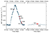 |
Fig. 1. Swift/BAT light curve of V 0332+53 during its 2015 outburst and at the time of the 2016 failed outburst. Times of NuSTAR observations are marked by the red points. |
The events extracted from these source and background regions were then used for spectral and timing analysis. To this aim, we used our developed analysis toolkit, detailed in (Ferrigno et al. 2023).
Here, we give a brief summary of the pipeline steps:
-
We filter out time intervals when the source shows extreme spectral or flux variability (e.g. dip, eclipse or flaring episodes).
-
We barycentre the arrival time of each event in the Solar System frame and performed a Lomb-Scargle (LS) search for coherent signals in the 3–7 keV range (this is usually already sufficient to find pulsations in case of bright pulsars). We take the highest peak in the LS spectrum as the preliminary spin frequency (Pspin), checking its consistency with the literature value.
-
We refine Pspin using an epoch folding search in a frequency interval around ±5% ×Pspin, after correcting for the binary motion, by using the binary orbital parameters taken from the Fermi Gamma-ray Burst Monitor (GBM) online database2 (Malacaria et al. 2020).
-
We extract folded pulse profiles with 128 phase-bins, in the 3–30 keV range, in intervals of 1500 s for the whole duration of the observation; we store these values in a time-phase matrix. We impose a minimum signal-to-noise ratio (S/N) of 15 for each time-selected folded profile and, when this threshold is not met, we sum adjacent profiles until obtaining the desired S/N.
-
We determine through a fast Fourier transform (FFT) the phase of the first harmonic in each time-selected pulse profile as a function of time. Subsequently, we examine the presence of a linear trend in the phase values and calculate a spin derivative term when the linear trend is significant at a confidence level greater than 95%. In this case, we adopt the new refined timing solution for further analysis.
-
We derive for the whole observation under exam an energy-phase matrix (a pulse profile for each energy bin) by folding data with the best spin and spin derivative values obtained from the previous step. There is a matrix associated with a specific Nbins, where Nbins is the number of the phase bins in the pulse profile (for example 8, 10, 16, or 32). The default energy spacing of the bins matches the intrinsic energy resolution of the FPMs. We compute separate source and background matrices for the two FPMA and FPMB detectors, and then sum the resulting matrices. For each energy bin, we compute the S/N of the pulse taking the background events into account. We then sum over adjacent bins to reach a minimum S/N over the whole NuSTAR energy band.
-
We compute the PF value in each re-binned energy bin, adopting the FFT method (see Ferrigno et al. 2023) and derive the harmonic decomposition simultaneously, which we also use in the following analysis:
 (2)
(2)Here ∣A0∣ is the average value of the pulse profile, which is the zero term of the FFT transform, and the terms A1...k are the k-th terms of the discrete Fourier transform, so that each ∣Ak∣ represents the amplitude of the k-th harmonic.
-
We truncate the Fourier spectral decomposition, using a number of harmonics that describe the pulse with a statistical acceptance level of at least 10% (usually 3–5 harmonics).
-
We compute the uncertainty on the PF value using a bootstrap method. For each energy-resolved profile, we simulated 1000 faked profiles, assuming Poisson statistics in each phase bin; we then derive the average and the standard deviation of this sample. After verifying that the average is compatible with the value computed from data, we adopt the sample standard deviation as an estimate of the uncertainty of the PF at a 1σ confidence level.
-
We compute the correlation and the lag spectra for each observation according to the methods described in Ferrigno et al. (2023), but slightly modifying the procedure to improve the error estimation (see Sect. 3.2). We use the 3–70 keV band, with the exclusion of the energy bin which we want to cross-correlate, as the band to extract the PP of reference.
For the spectral analysis, we used numkarf and numkrmf to obtain the ancillary response and the redistribution matrix files, respectively. We rebin the source spectra using the ftgrouppha tool3 optimisation algorithm of Kaastra & Bleeker (2016) and with the additional requirement of a S/N at least of three for each rebinned energy bin.
2.1. Energy and luminosity dependence of pulse profiles
An energy-phase map provides a quick visual overview of the energy-phase matrix. For each array of phase bin values, we calculate the average and standard deviation. A normalised pulse profile is then created by subtracting this average and dividing by the standard deviation for each phase bin value. These maps are also useful for identifying broad energy bands in which the pulse profiles exhibit the most pronounced variations. We show for example in the right panels of Fig. 2 two maps taken from the first two ObsID 802 and 804, which at once give an idea of the complex and strongly energy dependent changes in the PP, especially around the cyclotron line energy, at ECyc ∼ 28 keV, (see e.g. Tsygankov et al. 2006, for a comparison where similar maps were extracted from INTEGRAL data). The magenta lines show the energy ranges boundaries (2.4–10 keV, 10–22 keV, 22–32 keV, and 32–70 keV) from which some reference pulse profiles are extracted (right panels of Fig. 2). Similar plots for the other observations examined in this work are shown in Appendix A. It is evident that the profiles vary significantly in their harmonic content both as a function of energy and accretion state. Although the range of luminosity encompasses likely accretion states above and below the critical threshold, it is difficult to clearly identify a single component or pattern that might indicate a switch of the accretion mode.
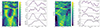 |
Fig. 2. Energy-phase colour maps and energy-selected pulse profiles for ObsIDs 802 and 804. |
2.2. Modelling the PFS
From a qualitative description of the pulse-energy dependence provided by the energy phase maps, we moved on to a quantitative description of the PP changes using the spectral decomposition of each profile. To this end, the study of the PFS provided the most robust way of tracking such changes, although their description is still phenomenological. Because we are mostly interested in accounting and describing the characteristics of the local features, we rely on a polynomial function to model the PF continuum as described in Ferrigno et al. (2023). To prevent the polynomial order to be too high and, thus, to avoid describing the shapes of local features with the polynomial continuum, we split the fit into two energy bands: a low- and a high-energy one. The energy where we split the modelling (Esplit) is chosen in the 10–15 keV range (i.e. sufficiently distant from typical cyclotron line energies). We use a spline function to interpolate the data points in this range and search for a zero in the period derivative. If such a value is found, Esplit is set to the corresponding energy bin, otherwise Esplit is set to the energy value corresponding to the minimum of the first derivative of the interpolating function. The polynomial order is chosen so that the fitted model has a corresponding p-value higher than 0.05.
In the low-energy band (typically between 3 and 12 keV), we do not find significant hints to features corresponding to the iron emission line in any of the observations (see details in Sect. 3.3), so that a simple, n-order polynomial is sufficient to reach a statistically acceptable fit.
In the high-energy part of the PFS, when local features are clearly spotted, we model them using Gaussian profiles, where the line centroid, the width and amplitude are free fitting parameters, after the fit seed values are set by eye. We caution the reader to not implicitly assume that Gaussian components with positive, or negative, amplitudes are direct analogues of emission, or absorption, lines as in the energy spectra. Our description of the PFS remains purely phenomenological and any tempting matching at a specific energy close to a spectral feature needs to be carefully examined case by case.
We use the lmfit python package (Newville et al. 2024) for obtaining the best-fitting parameters and calculating the associated uncertainties using Markov chain Monte Carlo (MCMC) algorithms from the emcee package (Foreman-Mackey et al. 2013). We use the Goodman & Weare algorithm (Goodman & Weare 2010) with 50 walkers, a burning phase of 600 steps, and a length of 6000, to prevent auto-correlation effects. From the sample, we extract the 50th, the 16th and the 84th percentile of the marginalised distributions as the best-fitting value and associated uncertainty. We report for each fit the reduced chi-squared value (χred2) and the corresponding degrees of freedom (d.o.f.).
As shown in Ferrigno et al. (2023), the PF spectrum slightly depends on the method by which the PF is calculated, on the number of phase-bins for the folded profiles and on the minimum S/N adopted to rebin the original PF spectrum (which is produced on a first instance at the instrumental spectral resolution) when needed. We found no general recipe which could be systematically applied, as much depends on the average value of the PF, on the source count rate and on the background level. We produced different PFS by varying all the possible criteria. For this source and the set of the observations that we analysed, we generally found that a S/N = 4 and a number of phase-bins of 16 provided the best compromise between S/N and spectral resolution. In a few cases, for better visual clarity, we excluded from the fit a Nexcl number of last bins, affected by larger uncertainties. We present a complete log of the observations and the parameters of the PFS used in this work in Table 1.
We apply the same pipeline (model fitting and error evaluations) and criteria to the description of the energy-dependence of the amplitudes of the first two harmonics. We report best-fitting results and uncertainties in the first and second labelled columns of Tables 2 and 3. We show the data, best-fitting models, and residuals in Appendix B.
Best-fit parameters for ObsID 802, 804, 806, and 808.
Best-fit parameters for PFS and ObsID 810, 902, and 904.
3. Pulsed fraction spectra fit results
We are able to satisfactorily describe, in statistical terms, the PFS using a very limited number of local components (either one or two) and polynomial functions of low order. A general picture of all the PFS, the best-fitting models and the residuals in units of standard deviations are shown in Figs. 3 and 4. The first four observations of Table 1 have sufficient statistics to allow a detailed view of the PF behaviour around the cyclotron line range (25–35 keV), while the remaining three observations have less statistics and do not allow a finer characterisation of the features. We report the best-fitting parameters and errors of the PFS, in the PF column of Tables 2 and 3.
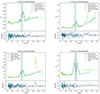 |
Fig. 3. PFS, best-fitting models, and residuals for ObsID 802, 804, 806, and 808. Cyan dashed lines mark the energy positions of the Gaussian peaks. The black line marks the energy of the fundamental cyclotron line (from Doroshenko et al. 2017). |
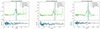 |
Fig. 4. Pulsed fraction spectra, best-fitting models, and residuals for ObsID 810, 902, and 904. Cyan dashed lines mark best-fitting energy positions of the Gaussian peaks. The black line marks the energy of the fundamental cyclotron line (from Doroshenko et al. 2017). |
All the examined PFS share some common characteristics, which can be assumed to weakly depend on the accretion state: the PF values below Esplit are generally very low (< 0.1), especially compared with other well-known accreting binaries (see e.g. Ferrigno et al. 2023), and tend to show a global minimum around 8–12 keV. After this minimum the PF starts to increase following a linear trend, which is then interrupted by the presence of a complex structure that we decided to model as two Gaussians with positive amplitudes. Although the modelling of this complex feature is not unique (for instance, a similar good fit is achieved by fitting with a broader Gaussian with positive amplitude and a narrower one with negative amplitude), the model we adopted appears to us better motivated both because PPs do significantly and rapidly change in this band (as we show in Sect. 3.1) and because this decomposition can be also linked to a physical interpretation of the energy spectra (see Sect. 4).
As shown in the four panels of Fig. 3, these two peaks show some variations in their relative amplitudes (see also Fig. 5, where PF data and best-fitting models for the four ObsID are superimposed), though their positions and widths remain always consistent within the uncertainties.
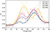 |
Fig. 5. Pulsed fraction spectra for the first four observations in the 20–36 keV energy band. The best-fitting models are superimposed (see Table 2). |
In the first four observations the positions of the two features do not display significant variations and their distance, relative to the spectral position of the fundamental cyclotron line (Doroshenko et al. 2017), remains constant as shown in Fig. 6. By reference to the peak position with respect to the cyclotron position, we shall refer to these PFS features as the red and blue (also left and right) peaks.
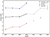 |
Fig. 6. Best-fitting peak energies of the PFS features and energies of the fundamental cyclotron line for the different observations. We report the cyclotron line energies from the spectral analysis of Doroshenko et al. (2017) (grey dots) and from this work (black dots). Red, blue and green points sign the best-fitting values from the PFS features, when two lines are clearly identified (red and blue dots) and when only one peak has been detected (green dots) (from Tables 2 and 3). |
After the blue peak, the PF values tend to increase again for the two brightest observations (802 and 804), while for all the remaining observations a lack of good statistics prevents us to determine any clear pattern.
The three observations at lower statistics (810, 902, and 904) in Fig. 4 still confirm the significant increase in PF around the cyclotron energy range, though we can only constrain the presence of a single peak (though some hints for a still more complex, double peaked profile, is suggested by the fact that at the best-fitting Gaussian peak energy, one, or more, data points remain always below the best-fitting model). The peak is clearly below the expected cyclotron line energy in the first two observations, while it is compatible just in ObsID 904. In this latter case the peak position error is larger and we guess a blending of the two features, if their amplitudes become comparable, is occurring. To have a comprehensive picture of all these results, we report all the peak positions for each ObsID in comparison with the spectral cyclotron line values in Fig. 6.
3.1. Changes in the pulse profile around Ecyc
We examine here the changes in PPs for selected energy ranges as derived from the modelling of the PF spectra. We note that a detailed description of the pulse shape requires a good number of phase bins (typically more than 10), which, however, might result in noisy profiles if the profiles are selected from too narrow energy intervals. To have enough statistics, but still preserving our objective to best describe the profile changes at the characteristic energies of the PF features, for each observation we extracted the PP using the best-fitting parameters in Table 2. For each clearly identified Gaussian line centred at Epeak, we selected the energy range from Epeak − σ and Epeak + σ. We show the results of the four ObsIDs where two peaks are present in Fig. 7, where we superimposed in the upper panels the two energy-selected profiles (red/blue colours show PP extracted from the red/blue peak energy ranges).
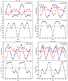 |
Fig. 7. Normalised energy-resolved pulse profiles for the ObsID 802, 804, 806, and 808. Upper panels show energy-selected profiles around the two PF peaks, lower panels show the full 3–70 keV energy-averaged PP. |
The red PP is characterised by a variable broad peak at phase ∼0.5. The peak broadens and its amplitude significantly increases as the luminosity decreases. The blue PP is more variable with the source luminosity, with its maxima and minima generally in phase opposition with those of the red peak. It is single peaked in the first two observations, there is a hint of a double peak in ObsID 806 and it becomes clearly double peaked in ObsID 808.
3.2. Cross and lag spectra around Ecyc
We computed the cross-correlation (CC, hereafter) and lag spectra for the first four observations (ObsID 802, 804, 806 and 808). To improve the quality of the spectra, we used PP with 16 phase-bins and a S/N of 6. We comprehensively show them in Fig. 8. As explained in Ferrigno et al. (2023), we computed the error-bars on these points by Monte-Carlo simulating N faked PP with the same Poisson statistics and taking the standard deviation from each set of simulations. We noted that some points were affected by larger uncertainties with respect to adjacent bins, due to the presence of some outliers in the distribution. To avoid this condition, we use here N = 125 faked PP and a trimmed standard deviation, where we rejected the left and right tails of the MC distribution at a 5% level. This choice drastically improved the quality of the spectra by significantly lowering the uncertainties (generally more than 50% in CC spectra, and a factor 3-4 for the lag spectra) and their interpretation.
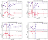 |
Fig. 8. Cross-correlation and lag spectra for ObsID 802, 804, 806, and 808. The spectra are shown in the high-energy (20–70 keV) range for highlighting the behaviour around the cyclotron line energies. The brown and blue vertical lines mark the positions of the best-fit Gaussians of the PFS. The vertical grey line mark the spectral best-fit position of the cyclotron absorption line (Doroshenko et al. 2016). Lags are given in phase units. |
3.3. Pulse profile changes in the low-energy band and at the iron line
Below 12 keV the PFS are quite peculiar if compared to the sources analysed in Ferrigno et al. (2023). In Fig. 9 we show the representative PFS for observations 802, 804, 806 and 808, which have the best statistics to search for local substructures. With the exception of 806, whose PF is flat in the entire low energy band, the other three spectra show a local peak between 3 and 6 keV. We expected to find a drop in the PF at energies around ∼6.4 keV, similarly to what observed in the PFS of the other sources with relatively broad (σ ∼ 0.4 keV) iron emission lines (Ferrigno et al. 2023). However, we found no evidence of a drop in PF values as clearly shown from the PFS shown in upper panels of Fig. 10. Similarly, the CC spectra (bottom panel of Fig. 10) do not show any significant change in the pulse profiles.
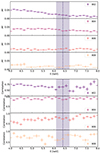 |
Fig. 10. Pulsed fraction values (upper panel) and CC spectra (lower panel) for ObsID 802,804,806 and 808 in the 4–9 keV energy range. The position and width of the spectral emission iron line is marked by the dotted line and the purple-coloured area (1-sigma contour). |
Bykov et al. (2021) reported that the iron emission line of V 0332+53 pulsates, based on an analysis of its 2004-2005 outburst observed with Rossi XTE. This suggests that part of the emission likely originates in the neutron star’s magnetosphere. Our findings align with this claim, as the iron line photons appear to be emitted coherently. The optical depth of the fluorescence process path is consistent with the main pulsation, implying that the reflector is either close to the primary hard emission source or that the pulsation is sufficiently long to maintain coherence or a combination of both cases. This may explain the lack of a significant dip in the PFS at these energies. However, a detailed analysis of the relationship between pulse profiles, shapes, and the intensity of the frequently observed iron fluorescence line in this and similar sources is beyond the scope of this paper and will be addressed in a future study.
4. Spectral analysis
Doroshenko et al. (2016) and Vybornov et al. (2017) have reported on the spectral analysis of these NuSTAR observations. The former performed phase-averaged spectroscopy, while the latter analysed pulse-resolved spectra. For this work, we do not aim to perform a new detailed spectral analysis of these datasets; instead, we investigate if, and how, the features we identified in the PFS might have possible spectral counterparts. We limit this analysis to the first four ObsID of Table 1 because of their higher statistics. First, we use the tools of the phase-resolved analysis in Sect. 4.1 to investigate the spectral distribution of the pulsed photons around the peaks of the energy-selected PPs. Because the PF is a measure of the ratio of the pulsed to the total emission (at a particular energy bin), this step will provide evidence that the shape observed in the PFS is linked to excess photons at the pulsed peak and their energy distributions are compatible with what is observed in the corresponding PFS. Moreover, this will also allow us to estimate the number of counts responsible for the observed peaks in the PFS.
In Sect. 4.2, we test a set of possible spectral decomposition of the phase-averaged spectrum using some constraints derived from the PFS modelling and the phase-resolved spectroscopy. The results of these steps will support a coherent interpretation of all our results linking the features in the PFS with spectral residuals around the cyclotron line energy.
4.1. Phase-resolved spectral characterisation of the peak excesses
To obtain a first-order estimate of the emission shape responsible of the pulse peak, we consider the PPs shown in Fig. 7. For each PP we visually identified the phase bin with the highest amplitude value, we selected a continuous phase interval expanding to the neighbour phase bins with largest amplitudes for a total of 4 phase bins. From these bin intervals we derived a phase range for extracting the peak pulse spectrum. We then selected the bin with the lowest amplitude value and derived the phase interval using the same logic as for the peak pulse spectrum to extract a corresponding background pulse spectrum. We choose this fixed range of phase intervals because the peak phase and the bottom part of the PP are thus uniformly covered for all the PPs examined.
We used xspec and χ2 statistics to fit the peak pulse spectrum using the background pulse spectrum as background and the addspec tool4 to sum the FPMA and FPMB spectra and corresponding background and response files.
We noted positive excesses around the expected energies of the Gaussian peaks of the PF spectra. We fitted them using a simple Gaussian model in the restricted energy bands 22–28 keV and 28–36 keV for the red and blue peaks, respectively. In all cases, we found satisfactory reduced χ2 for all fits performed.
We show in Fig. 11 the data and the best-fit model for the four datasets. In Table 4, we compare the best-fitting values from the phase-resolved spectral fits and the best-fitting parameters of the PF spectra (same as Table 2). The parameters are generally well in agreement within the statistical uncertainties.
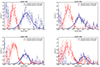 |
Fig. 11. Spectral characterisation of the phase-resolved peak excesses for ObsIDs 802, 804, 806, and 808. Each panel shows the photon excesses per energy bin for the blue (blue data) and the red peak (red data). The Gaussian best-fitting model for the red (blue) dataset is marked by a thick red (blue) line. |
As a consistency check, we evaluated if the number of counts in these excesses are sufficient to account for the increase in the blue/red peaks of the PFS. The number of excess photons in the spectra is simply the line normalisation multiplied by the exposure time (see Table 1) and the effective area (we take this value in correspondence with the Gaussian peak energies, as the effective area is nearly constant for this narrow energy range). We, then, multiplied this number by a corrective factor of 0.9 (which we derived through simple simulations to convert the number of photons into counts, and therefore compensate for the effects of the redistribution matrix). The excess counts are reported in the seventh column of Table 4.
Comparison of best-fitting values for the red and blue peaks of the PFS versus phase-resolved analysis of count excesses.
The number of counts in the PFS is obtained by element-wise multiplication of the best-fitting Gaussian model values with the total number of counts for each energy bin, and then summing over the values of the resulting vector. Because PF values depend on the method how the PF is actually computed, we double checked these values adopting also the PF area definition (see PFS comparisons in the appendix of Ferrigno et al. 2023), as this method gives the most direct way to count the number of pulsed photons in the profile. We found that both PF definitions led to consistent estimates, and we report the values, obtained with the FFT method, in Table 4.
The number of counts from this spectral excess analysis and the ones observed in the PF feature are of the same order of magnitude, and in most cases, even consistent within the error bars. Given the rough approximations used for this comparative analysis, we retain that the local increase in the PF can be attributed to a certain increase in pulsed photons which have a clear and local energy range distribution.
4.2. Spectral analysis: modelling the phase-averaged spectra
Based on the results of the phase-resolved spectroscopy, which clearly showed that characteristic emission features can be associated with the pulsed part of the emission at the energies of the PF blue and red peaks, we evaluate here the conditions under which such emission peaks at the two sides of the broad absorption CRSF can be statistically detected in the phase-averaged spectra. As our main interest lies mostly in the high-energy part of the spectrum, we fitted the data in the 5–60 keV energy range and analysed only the first four observations, which have good statistics. We used the W statistics, analogue to the Cash statistics (C-stat) when a background dataset is provided, assuming Poisson distributions for both source and background spectra (see Sect. 7 in Arnaud et al. 2011). We performed an initial fit with the usual minimisation algorithm and explored the neighbouring parameter space with a Monte Carlo Markov Chain MCMC, using the Goodman & Weare algorithm Goodman & Weare (2010) with 200 walkers, a burn-in phase of 20 000 and a length of 200 000 steps. We visually inspected the fit statistic distribution and the parameter corner plots to verify that the chains converged properly.
We model the continuum using a power-law with a high-energy cut-off (highecut) smoothed with a third-order polynomial at the cut-off to avoid the artificial discontinuity created by the model (newhcut component, as defined in Burderi et al. 2000). This phenomenological approach has been extensively used in literature for a long time, though it is well known to be an approximation to the true continuum shape. We are aware that other phenomenological and even some physical continuum models are available. However, as we discuss later, our aim is to evaluate the statistical significance of these possible detection and their correlation with the broad and deep CRSF.
We used the tbabs component for the photo-electric Galactic extinction. Because the value of the Galactic absorption column parameter, NH, is poorly constrained, we fixed it to the expected interstellar value5 of 7 × 1021 cm−2.
All spectra clearly showed the presence of two CRSF, at ∼28 keV and ∼51 keV. The use of a single absorption Gaussian (gabs model in Xspec) to model these CRSFs resulted always in poor fits (see Table 5) and evident residuals especially around the fundamental line, thus indicating a complex spectral shape of this feature. We refer to this model as the ‘one Gabs’. As already noted by Pottschmidt et al. (2005), the cyclotron profile of V 0332+53 is, at least phenomenologically, better described by two nested Gaussian absorption lines, that is a superposition of a shallow/narrow core and a broader/deeper Gaussian wing. We noted no statistically significant shift between the energies of these two absorption lines, and therefore, we tied these positions to be the same in the best-fitting model. We refer to this model as the ‘nested Gabs’. In general, also for the NuSTAR spectra, this model gives a significant statistical improvement with respect to the one Gabs model. Finally, based on the hints from the PF spectrum modelling and the phase-resolved analysis, we modelled the CRSF using a broad absorption Gaussian with two, narrower, Gaussian emission lines: one above and one below the absorption line energy, we shall refer to this as the ‘wings’ model. To avoid over-fitting and model degeneracy, we impose Gaussian priors on the centroid energy and width of the emission lines from the phase-resolved spectroscopy as described in Sect. 4.1. For the other spectral parameters, we use non-informative priors in linear or logarithmic space, as appropriate. The tables in Appendix C show the best-fitting parameters and uncertainties of these three models, while we give a quick comparative view of the best-fit results (C-stat values and d.o.f.) in Table 5. The posterior error distributions of all the spectral parameters of this model appear generally well constrained (corner plots of the posterior error distributions of the four fits are presented in Appendix D).
Quick-look summary fit report.
We use the Akaike information criterion (AIC; Akaike 1974) to evaluate the statistical improvements of the nested Gabs and wings model with respect to the one Gabs model. The AIC values are defined according to the formula:

where k is the number of fitted parameters of the model and ℒmax is the maximum likelihood value. The C-statistics value and the maximum likelihood are related as Cstat = −2ln(ℒmax) (Cash 1979). We calculate the AIC difference (ΔAIC) over all candidate models with respect to the simpler, one Gabs model. Models with ΔAIC ≫ 10 are strongly more favoured with respect to the baseline model. The wings model is always statistically more favoured with respect to the one Gabs model, whereas the nested Gabs model is the preferred model in the first three observations, but it is the least statistically significant one for spectrum 806. In three, out of four spectra, the nested Gabs model is statistically favoured over the wings model, although we noted that such improvement can be mostly attributed by a better description of the overall continuum shape, whereas residuals at the cyclotron line energy are distributed similarly in both models.
For the wings model, the best-fit normalisations (or the upper limits, when lines are not statistically detected) of the emission lines give a total number of photons in the line that is a factor of 2-3 higher than the excess counts derived from the phase-resolved analysis (last column of Table 4). This is not surprising, given the systematic large uncertainties which are involved in the choice of the phase intervals for the excess analysis and in subtracting, or disentangling, the absorption component of the CRSF profile. In conclusion, we retain these count estimates to be satisfactorily in agreement.
4.3. Spectral analysis: phase-resolved spectroscopy of ObsID 806
As a final step in establishing a relationship between the spectral blue and red line components and the features of the PFS we looked for phase-dependent changes of the line fluxes. If these spectral lines are responsible for the local increase in the PF and their pulsed emission is clearly peaked at some spin phase, we expect a corresponding modulation of the fluxes. To test this conclusion, we took the ObsID 806 where both spectral lines are clearly detected and their line normalisations are the highest. We phase-resolved the spectra using ten equally spaced phase bins and applied to these spectra the wings spectral model, assuming the same priors of the phase-averaged analysis and calculating the best-fitting parameters and errors.
In Fig. 12, we illustrate the variation of line normalisations across the spin phase. For improved clarity, we overlay the energy-resolved pulse profiles from Fig. 7, specifically those extracted in the 24.1–27.1 keV range for the red peak and the 28.3–32.4 keV range for the blue peak.
 |
Fig. 12. Phase-resolved spectroscopy for ObsID 806. Left (Right) panel: phase-dependence of the red (blue) line normalisation (black dots in units of 10−4 photons/cm−2/s) superimposed with the energy-resolved pulse-profile (from Fig. 7). |
The modulations are clearly visible and there is a remarkable good match with the corresponding pulse profiles. In conclusion, we find that there is a consistent and robust picture that from the features that appear in the PFS of V 0332+53 lead to a complex but well-consistent modelling of the energy spectra around the fundamental cyclotron line energy. We emphasise that such modelling is yet based on a phenomenological approach and the true cyclotron line shape might be certainly more complex than what is envisaged here (a mix of emission/absorption Gaussians at different energies). However, this modelling would have been difficult to do at all had it not been for the analysis of the energy-resolved PFS.
5. Discussion
We presented a comprehensive analysis of the variations of the pulse profile with energy of the accreting X-ray pulsar V 0332+53, using observations from NuSTAR, which is today’s best observatory to perform this kind of study in the 3–70 keV band at the highest energy resolution. Compared to the majority of other well known X-ray pulsars, V 0332+53 has a remarkable PFS, whose main characteristics seem to only mildly depend on the accretion rate. The examined dataset span a wide range of luminosity: from something close to the Eddington limit (LEdd = 2 × 1038 erg s−1 for a classical 1.4 Msun NS, e.g. ObsID 802) to observations when the luminosity was only a few percent of the Eddington limit (e.g. ObsID 904). In all cases, the PF values are generally low in the soft (3–10 keV) and in the intermediate (10–22 keV) X-ray bands, followed by a significant increase only around the energy of the fundamental cyclotron line. Above the cyclotron energy range we note the only significant change with luminosity, as the PF trend values tend to flatten as the luminosity decreases (see Figs. 3 and 4). Contrary to what observed in other sources, where the PFS dip around the cyclotron line energies (see Ferrigno et al. 2023), V 0332+53 shows a peculiar wiggle, which could be described, in the most simple terms, as two close Gaussian lines with positive amplitudes. The fact that this pattern is similarly reproduced in four different datasets is evidence that the shape has a physical origin, and cannot be due to statistical fluctuations.
Tsygankov et al. (2006) gave a detailed description of the profile variations with energy of this source, noting both the abrupt shape change below and above the cyclotron energy and the PF increase at these energies. We were able to resolve spectrally this increase by showing how it appears complex overall when compared with PFS of other similar sources (see e.g. Ferrigno et al. 2023). One might, however, argue that a drop in the PF values is still present in-between the two lines, albeit the bottom value of the PF appears consistent with the expected trend of the underneath continuum. However, the fact that these two peaks are physically not connected is supported by the evident change of the pulse profile shapes (Fig. 5) and by the clear trends in the CC and lag spectra (Fig. 8) that show how the discontinuity of the shape is produced around the cyclotron line energy: the lag profile drifts rapidly, yet continuously, in phase with the steepest derivative very close to the cyclotron line energy. This can also be appreciated by looking at the energy maps (see Fig. 2), where the drift of the PP peak in the 22–32 keV range is clearly visible. The spectral shape of the pulsed photons responsible of these local PF peaks adds another piece of evidence of their uncommon origin. The Gaussian shaped distribution of excess photons, as derived by their respective energy-resolved peaks in pulse profiles, have spectral widths that well match the red and blue PF Gaussian widths, with little leakage from adjacent energy ranges, apart from some red photons in the blue energy range for ObsID 808 (Fig. 11).
The trend of the peak positions with source luminosity as shown in Fig. 6 trails the trend of the cyclotron line energy: the energy of the peaks remains always on the two sides of the cyclotron line, though there is no clear correlation with source luminosity. The ratio of the peak amplitudes, on the contrary, varies: as the source luminosity decreases the red peak amplitude increases, whereas the blue peak amplitude does not display significant variability, as shown in Fig. 5, though a shift of about 1 keV is hinted in ObsID 808.
5.1. Physical origin of the PFS peaks
After having established the general properties of these features, we discuss their possible physical origin. As noted for many other sources (see e.g. Ferrigno et al. 2011), a sharp pulse change at the cyclotron energy is expected because of the complex and sharp resonant cross-section energy-dependence of the cyclotron absorption for the extra-ordinary mode photons, while ordinary mode photons are not affected. Because the relative fraction of ordinary vs extra-ordinary mode photons might be a function of energy and there are preferential angles for both modes according to the energy at which the scattered, or re-emitted, photon, is escaping, the pulse shape can be fundamentally altered. Thus, as the shape changes, a change in the pulse amplitude (and consequently in the PF value) is expected. In consideration of their peak energies, variability, and associated energy-dependent, pulse shapes, we therefore retain the two peaks in the PFS related with the physical processes that also produce the CRSF. The next step is to ask why these features produce an increase the PF values, rather than to decrease it with respect to what is observed in other sources. Ferrigno et al. (2023) showed the consistency between the cyclotron energies as derived by the spectral analysis and the position of the absorption features in the PFS for the four sources analysed (e.g. Cen X–3, 4U 1626–67, Her X–1 and Cep X–4), while for V 0332+53 the mismatch in the positions is evident: none of the two features can be reliably appointed to the spectral energy position ECyc. However, theoretical models of cyclotron line absorption have since long time pointed out that the absorption profile is far from being either a smooth Gaussian, or a Lorentzian, and many physical processes intervene to distort the profile (Isenberg et al. 1998a; Schönherr et al. 2007; Schwarm 2017). One key prediction has been the presence of line wings. Such features would appear in emission with respect to a simpler Gaussian profile fit and MC simulations have confirmed the formation of these structures on both sides of cyclotron energy (see references in Sect. 1) in certain conditions.
As a next step, we attempted to find a spectral confirmation to this scenario. To this aim, we first looked at the spectral shape responsible of the pulsed part of the profile for each PF peak. We found (as expected) a good agreement between the PF shape and the count excesses shape (Fig. 11). Interpreting these excesses as the source of the wings components (here simply modelled as Gaussian emission features), we reexamined the phase-averaged energy spectra of the first four NuSTAR observations. We found that residuals around the fundamental CRSF are always present. We also made different spectral fits by changing both the continuum shapes and the line shapes and noted that residuals were always there. On the contrary, Doroshenko et al. (2017) fitting the same data found no evidence for significant residuals beyond a simple Gaussian fit; we were able to obtain very similar best-fitting parameters as the ones shown in Doroshenko et al. (2017), though in all cases the reduced χ2 were much worse. We argue that this is due to how the original spectra were re-binned. We used the optimal binning prescription from Kaastra & Bleeker (2016) to avoid oversampling the spectra, whereas Doroshenko et al. (2017) used the simpler requirement of a minimum 25 counts per noticed channel, thus resulting in spectra with ∼ a factor 4 more channels than the ones used by us. We note that over-sampled spectra have generally lower reduced χ2, which can lead to miss some residual patterns, especially if they are restricted to a narrow energy range.
We retain that these spectral residuals provide instead good evidence for a complex cyclotron line shape, and we showed that the addition of these emission lines as the ones found from the phase-resolved spectroscopy analysis gives generally a statistically significant improvement with respect to the null model (here the one Gabs model). However, we also note that by allowing the absorption line shape to take two additional free parameters (as shown with the nested Gabs model), the statistical description of the data could be even better and the need to add additional components around the energy of the fundamental CRSF appears no longer motivated.
This fact is clearly comprehensible if we make some computations on the relative flux components involved in the spectral components of the fits. For instance, if we take the best-fitting model wings (Table C.2) for ObsID 804, where there is good statistics for both the emission lines, and compute the best-fitting flux model in the energy range Ecyc − 2 × σcyc and Ecyc + 2 × σcyc (21.1–35.5 keV), we see that the cyclotron feature absorbs about half of the total emitted flux in this range, while the two emission lines contribute for only 2% to the total flux. It is therefore not surprising that by adding complexity to how the broad and deep absorption feature is modelled, any detection claim for such, relatively small, feature by means of pure spectral analysis becomes challenging (leaving aside that inherent complexity of finding a suitable spectral continuum). If this also applies to past observations of V 0332+53, we can understand how previous attempts to find evidence of such emission wings in the energy spectra of this source proved hard to succeed. The prominent peaks in the PFS raise questions about whether this behaviour is supported by theoretical radiative transfer models and what is the physical mechanism behind the significant increase in the pulsed fraction. Theoretical predictions for pulse profile formation rely on complex dependencies from multiple factors such as system geometry, light bending, and location of the regions of spectral formation (Falkner 2018), but, to our knowledge, no predictive quantitative assessment has been made regarding the expected fractional pulsed energy dependency for complex CRSF shapes with wings. Observationally we see that photons in the wings exhibit greater coherence than those of the underneath continuum. This suggests that the last scattering region of the wing photons, or their emission cone, is distinct and likely more asymmetric than the region producing the pulsed continuum. Some theoretical considerations play a role in this context. Assuming photons appearing in wings are spawned from higher excited Landau levels, then the escape beam pattern are different in case the electron de-excites from the first to ground state, or from the third to the second (Schwarm et al. 2014). Assuming that the red wing is mainly populated by spawned photons from third to second excited state (the observed energy difference of the second and fundamental cyclotron line energies is close to the red peak energy), and the blue wing by the transition from the first to the ground state, then the escape paths of these photons might also result in some phase shift, depending on the overall angles that the escape cones make with the observer’s line of sight and the assumed system geometry. Arguably we might intercept rescattered and spawned photons populating the red wing with their emission cone only from one column, while we intercept the blue photons, having a different beam angle only from the opposite column, thus explaining the large (almost 180°) phase shift observed in the energy-resolved pulse profiles extracted from the two features energy ranges (Fig. 5).
It remains also to be addressed the expected variations in the PFS around the cyclotron line for different luminosities (e.g. sub-critical luminosity vs supercritical luminosity regime). In this case, we did not find clear theoretical predictions to be compared and this is certainly an interesting avenue for future work.
5.2. System geometry
We need to address the question on what makes V 0332+53 so peculiar among all the other X-ray pulsars. Based on our knowledge, there is no other known source with the same set of characteristics as this one: very low PF values below the cyclotron line energy, strong PF increase and drastic pulse profile change at the cyclotron energy, extreme depth of the cyclotron line in the energy spectrum. This set of characteristics does not depend on the accretion rate, as we found these characteristics ubiquitous in all examined dataset. The NS magnetic field value, spin period, system physical orbital parameters, and the general spectral shape are standard when compared to the whole HMXB sample (Kim et al. 2023). We retain that the only key factor to possibly differentiate this source from all the others might be the geometrical factor: it is possible that our line-of-sight is well aligned with the spin axis, while the magnetic obliquity (i.e. the angle between the spin and the magnetic axis), has an extreme value, either very low, or close to be orthogonal.
Let us first consider the low spin axis angle hypothesis: even if the posterior probability of such geometry is very low, when considering the whole sample of known HMXBs, such probability becomes no longer marginal. If we take the most recent mass function estimate (fM = 0.44(1)M⊙ Doroshenko et al. 2016), and we assume a canonical 1.4 M⊙ NS mass and a possible mass range of 15–30 M⊙ for the companion star (an unevolved O8–9Ve star Negueruela et al. 1999), we obtain a very narrow range for the system inclination angle i = 14–19 deg, thus validating this first assumption.
Regarding the magnetic obliquity, let us first consider the orthogonal rotator case. This geometry needs to assume a fan beam pattern for all observations; this can explain at the same time the overall low PF values (most likely driven by inhomogeneous reflection patterns on the NS by the two accretion columns as seen by the distant observer) and the large optical depth of the cyclotron line in the energy spectra (most of the observed photons are observed coming perpendicularly to the magnetic field, where the scattering/absorption cross-section for cyclotron absorption is the highest). On the contrary, in the case of a small obliquity, less than 30° (a geometrical configuration that has been also independently advocated in a recent study, see Mushtukov et al. 2024), a pencil beam pattern for all observations must be assumed. To illustrate the feasibility of such geometry, we provide an example of simulated phase-energy maps. For this, we utilise a physical model for emission from a slab of highly magnetised plasma on the surface of a NS, as presented in Sokolova-Lapa et al. (2023). The simulations are based on a radiative transfer code, which addresses the formation of both the continuum and the cyclotron resonance. We chose a model described there as “inhomogeneous accretion mound”, which includes a variation of the density profile with depth but assumes the constant electron temperature and magnetic field strength throughout the emission region. Here, we fix the electron temperature to 7 keV and the magnetic field to 3.4 × 10¹² G, corresponding to a cyclotron energy of 30 keV. To study the variation of the observed signal with geometry (i.e. the observer’s inclination and the location of the emission regions), we combine the obtained emission, determined for a wide range of photon energies and angles to the magnetic field, with a relativistic ray-tracing code by Falkner (2018). This code calculates the projection of a rotating neutron star with defined emitting regions onto the observer’s sky, assuming the Schwarzschild metric. We chose a simple setup of two emitting identical poles on the neutron star surface. Figure 13 shows simulated phase-energy maps for the observed emission for two distinct geometries, chosen to illustrate two principally different results. The left-hand side indicates a striking variation of emission patterns in different energy bands, emphasised by a chosen geometry. The (fundamental) cyclotron line appears in the observed phase-averaged spectra at around 25 keV, affected by gravitational redshift and, to a smaller degree, by angular variability of the line profile. From this example, it is clear that a wide region around the cyclotron line energy – red and blue wings – is affected by redistribution much stronger than the line core. While the energies below (∼18–25 keV), corresponding to the red wing, show relatively weak, although noticeable phase shift, for a wide range of energies contributing to the blue wing, the structure of the map changes dramatically. We attribute this difference to more enhanced redistribution of photons into the blue wing during the line formation due to the relatively high electron temperature, as well as to the geometrical effect.
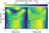 |
Fig. 13. Phase-energy maps simulated from the solution of radiative transfer equation in a slab of highly magnetised plasma based on a model described by Sokolova-Lapa et al. (2023) and combined with relativistic ray tracing by Falkner (2018). A colour map shows the variation of a normalised total observed flux. The two maps are calculated for observer’s inclinations i and the same location of two identically emitting poles, specified by their polar angle from the spin axis Θ and their azimuthal separation ΔΦ (the values are indicated on the panels). For the geometry displayed on the left, phase shifts occur over a broad range around the line, being caused by the redistribution of photons in the wings. The blue wing is particularly strongly affected by the process due to relatively high electron temperature kT = 7 keV. |
The right-hand panel presents the same geometry of the poles with the larger observer inclination, which result in almost completely aligned magnetic and spin axes. This configuration leads to a very low variability of the flux in a phase-energy map, including the cyclotron line region. Our simulations indicate a strong dependency of phase-energy maps on the assumed geometry. In this setup, the offset larger than ∼10° is required to create complex variation of the emission with the phase.
However, a thorough exploration of the parameter space is required to draw further conclusions, which will be presented in a future work. The presented maps serve exclusively to illustrate the effect of a complex angular behaviour of emission from a warm, strongly magnetised plasma, as expected close to the surface of the accreting NS. This affects not only the cyclotron line but also a broad range of surrounding energies, due to significant redistribution in the line wings. With these simulations, we aim to support the general interpretation of the emission wings presented in this work and highlight the primary influence of geometry on their phase variability. We remark that incorporating additional physical processes into the model – such as bulk, in addition to thermal Comptonisation, and a more realistic vertical extension of the emission region – is necessary to fully describe the complex accretion picture in the super-critical regime (see also Zhang et al. 2022).
In conclusion, both scenarios require that the emission mode, either fan or pencil, remains largely the same from all the examined observations, which likely encompass both super- and sub-critical regimes, thus also explaining the lack of significant changes in the observed PFS for observations at low and high accretion rates.
Interestingly, recent spectro-polarimetric observations of accreting pulsars seem to suggest that the rotational and magnetic angle are distributed according to such bimodality: either sources are orthogonal (like X–Persei and GRO J1008–57 Mushtukov et al. 2023; Tsygankov et al. 2023), or show a very small magnetic obliquity (like Cen X–3 and Her X–1 Doroshenko et al. 2022; Tsygankov et al. 2022). Future polarimetric observations of V 0332+53 will therefore be key to definitively determine the source’s geometry.
An open question remains the robustness of the correlation of the cyclotron line energy with the source luminosity (Tsygankov et al. 2006; Cusumano et al. 2016; Doroshenko et al. 2016; Ferrigno et al. 2016). We retain that the complexity of the line profile, taking into account the presence of wings on both side of the absorption feature, might not significantly alter the determination of the cyclotron line energy, although a deeper spectral analysis investigation with ad hoc physical modelling of the line (e.g. using the most recent MC codes Schwarm et al. 2017) is required for a definitive proof.
6. Conclusions
In this paper, we present an in-depth study of the variations in the pulse profile of V 0332+53 with energy using all available NuSTAR observations to date. Remarkable profile variations are observed on both sides of the putative fundamental cyclotron line energy (Ecycl ∼ 28 keV), which we interpret as features arising from the reprocessing of cyclotron line photons (either scattered or spawned from higher excited Landau levels) in the line-forming region. Consistent with previous theoretical predictions of how cyclotron lines should appear to the distant observer, we associate these profile changes to the emergence of the so-called cyclotron line wings. We infer that V 0332+53 is a source seen at low inclination angle and the magnetic axis direction is either ≲30° or is perpendicular to the rotational spin axis. Preliminary theoretical work shown in this paper supports our observational findings, though a detailed determination of all the physical ingredients in the line-forming region is deferred to a future publication. A robust physical model of cyclotron line shapes in V 0332+53 is needed in order to firmly test any correlation between cyclotron energy position and other observables, such as the source luminosity, as this in turn has key physical implications for the determination of the cyclotron line-forming region (Loudas et al. 2024). Finally, we hope that this work will encourage authors to model the energy-pulse shape dependence in their Monte Carlo radiative-transfer calculations, taking proper account of light propagation, as this work highlights the power of this method to identify and study the CRSF profile, which in principle encode important information about the plasma properties in the line-forming region.
Data availability
The appendices of this paper are accessible on Zenodo at https://zenodo.org/records/14471705.
Acknowledgments
The authors would like to acknowledge and thank Domitilla De Martino and Jakob Stierhof for very useful comments and discussion. This research was supported by the International Space Science Institute (ISSI) in Bern, through the ISSI Working Group project Disentangling Pulse Profiles of (Accreting) Neutron Stars. This research benefited from funding by the Space Science Faculty of the European Space Agency. The research has received funding from the European Union’s Horizon 2020 Programme under the AHEAD2020 project (grant agreement n. 871158). AD, EA, GC, VLP acknowledge funding from the Italian Space Agency, contract ASI/INAF n. I/004/11/4. CP, MDS, AD, FP, GR acknowledge support from SEAWIND grant funded by NextGenerationEU. ESL acknowledges support from Deutsche Forschungsgemeinschaft grant WI 1860/11-2. FP, AD, MDS, GR and CP aknowledge the INAF GO/GTO grant number 1.05.23.05.12 for the project OBIWAN (Observing high B-fIeld Whispers from Accreting Neutron stars). CM acknowledges funding from the Italian Ministry of University and Research (MUR), PRIN 2020 (prot. 2020BRP57Z) “Gravitational and Electro magnetic-wave Sources in the Universe with current and next generation detectors (GEMS)” and the INAF Research Grant Uncovering the optical beat of the fastest magnetised neutron stars (FANS). We made use of Heasoft and NASA archives for the NuSTAR data. We developed our own timing code for the epoch folding, orbital correction, building of time-phase and energy-phase matrices. This code is based partly on available Python packages such as: astropy (Astropy Collaboration 2022), lmfit (Newville et al. 2024), matplotlib (Hunter 2007), emcee (Foreman-Mackey et al. 2013), stingray (Bachetti et al. 2023), corner (Foreman-Mackey 2016), scipy (Virtanen et al. 2020). An online service that reproduces our current results is available on the Renku-lab platform of the Swiss Science Data Centre at this link.
References
- Akaike, H. 1974, IEEE Trans. Autom. Control, 19, 716 [Google Scholar]
- Araya, R. A., & Harding, A. K. 1996, A&AS, 120, 183 [NASA ADS] [Google Scholar]
- Araya, R. A., & Harding, A. K. 1999, ApJ, 517, 334 [NASA ADS] [CrossRef] [Google Scholar]
- Arnason, R. M., Papei, H., Barmby, P., Bahramian, A., & Gorski, M. D. 2021, MNRAS, 502, 5455 [NASA ADS] [CrossRef] [Google Scholar]
- Arnaud, K., Smith, R., & Siemiginowska, A. 2011, Handbook of X-ray Astronomy (Cambridge, UK: Cambridge University Press) [CrossRef] [Google Scholar]
- Astropy Collaboration (Price-Whelan, A. M., et al.) 2022, ApJ, 935, 167 [NASA ADS] [CrossRef] [Google Scholar]
- Bachetti, M., Huppenkothen, D., Khan, U., et al. 2023, https://doi.org/10.5281/zenodo.7970570 [Google Scholar]
- Basko, M. M., & Sunyaev, R. A. 1976, MNRAS, 175, 395 [Google Scholar]
- Baum, Z. A., Cherry, M. L., & Rodi, J. 2017, MNRAS, 467, 4424 [NASA ADS] [CrossRef] [Google Scholar]
- Becker, P. A., & Wolff, M. T. 2022, ApJ, 939, 67 [NASA ADS] [CrossRef] [Google Scholar]
- Beloborodov, A. M. 2002, ApJ, 566, L85 [Google Scholar]
- Burderi, L., Di Salvo, T., Robba, N. R., La Barbera, A., & Guainazzi, M. 2000, ApJ, 530, 429 [NASA ADS] [CrossRef] [Google Scholar]
- Bykov, S. D., Filippova, E. V., Gilfanov, M. R., et al. 2021, MNRAS, 506, 2156 [NASA ADS] [CrossRef] [Google Scholar]
- Canuto, V., & Ventura, J. 1977, Fund. Cosmic Phys., 2, 203 [NASA ADS] [Google Scholar]
- Cash, W. 1979, ApJ, 228, 939 [Google Scholar]
- Cusumano, G., La Parola, V., D’Aì, A., et al. 2016, MNRAS, 460, L99 [NASA ADS] [CrossRef] [Google Scholar]
- Doroshenko, V., Tsygankov, S., & Santangelo, A. 2016, A&A, 589, A72 [NASA ADS] [CrossRef] [EDP Sciences] [Google Scholar]
- Doroshenko, V., Tsygankov, S. S., Mushtukov, A. A., et al. 2017, MNRAS, 466, 2143 [NASA ADS] [CrossRef] [Google Scholar]
- Doroshenko, V., Poutanen, J., Tsygankov, S. S., et al. 2022, Nat. Astron., 6, 1433 [NASA ADS] [CrossRef] [Google Scholar]
- Falkner, S. 2018, Ph.D. Thesis, Friedrich Alexander University of Erlangen-Nuremberg, Germany [Google Scholar]
- Ferrigno, C., Falanga, M., Bozzo, E., et al. 2011, A&A, 532, A76 [CrossRef] [EDP Sciences] [Google Scholar]
- Ferrigno, C., Pjanka, P., Bozzo, E., et al. 2016, A&A, 593, A105 [NASA ADS] [CrossRef] [EDP Sciences] [Google Scholar]
- Ferrigno, C., D’Aì, A., & Ambrosi, E. 2023, A&A, 677, A103 [NASA ADS] [CrossRef] [EDP Sciences] [Google Scholar]
- Foreman-Mackey, D. 2016, J. Open Source Software, 1, 24 [NASA ADS] [CrossRef] [Google Scholar]
- Foreman-Mackey, D., Hogg, D. W., Lang, D., & Goodman, J. 2013, PASP, 125, 306 [Google Scholar]
- Goodman, J., & Weare, J. 2010, Commun. Appl. Math. Comput. Sci., 5, 65 [Google Scholar]
- Harding, A. K., & Daugherty, J. K. 1991, ApJ, 374, 687 [NASA ADS] [CrossRef] [Google Scholar]
- Harrison, F. A., Craig, W. W., Christensen, F. E., et al. 2013, ApJ, 770, 103 [Google Scholar]
- Honeycutt, R. K., & Schlegel, E. M. 1985, PASP, 97, 300 [NASA ADS] [CrossRef] [Google Scholar]
- Hunter, J. D. 2007, Comput. Sci. Eng., 9, 90 [NASA ADS] [CrossRef] [Google Scholar]
- Isenberg, M., Lamb, D. Q., & Wang, J. C. L. 1998a, ApJ, 493, 154 [NASA ADS] [CrossRef] [Google Scholar]
- Isenberg, M., Lamb, D. Q., & Wang, J. C. L. 1998b, ApJ, 505, 688 [NASA ADS] [CrossRef] [Google Scholar]
- Kaastra, J. S., & Bleeker, J. A. M. 2016, A&A, 587, A151 [NASA ADS] [CrossRef] [EDP Sciences] [Google Scholar]
- Kim, V., Izmailova, I., & Aimuratov, Y. 2023, ApJS, 268, 21 [NASA ADS] [CrossRef] [Google Scholar]
- Kumar, S., Bala, S., & Bhattacharya, D. 2022, MNRAS, 515, 914 [CrossRef] [Google Scholar]
- Kylafis, N. D., Trümper, J. E., & Loudas, N. A. 2021, A&A, 655, A39 [NASA ADS] [CrossRef] [EDP Sciences] [Google Scholar]
- Langer, S. H., & Rappaport, S. 1982, ApJ, 257, 733 [NASA ADS] [CrossRef] [Google Scholar]
- Loudas, N., Kylafis, N. D., & Trümper, J. 2024, A&A, 685, A95 [NASA ADS] [CrossRef] [EDP Sciences] [Google Scholar]
- Lutovinov, A. A., Tsygankov, S. S., Suleimanov, V. F., et al. 2015, MNRAS, 448, 2175 [NASA ADS] [CrossRef] [Google Scholar]
- Makishima, K., Mihara, T., Ishida, M., et al. 1990, ApJ, 365, L59 [NASA ADS] [CrossRef] [Google Scholar]
- Malacaria, C., Jenke, P., Roberts, O. J., et al. 2020, ApJ, 896, 90 [NASA ADS] [CrossRef] [Google Scholar]
- Mowlavi, N., Kreykenbohm, I., Shaw, S. E., et al. 2006, A&A, 451, 187 [NASA ADS] [CrossRef] [EDP Sciences] [Google Scholar]
- Mushtukov, A. A., Suleimanov, V. F., Tsygankov, S. S., & Poutanen, J. 2015, MNRAS, 454, 2539 [Google Scholar]
- Mushtukov, A. A., Verhagen, P. A., Tsygankov, S. S., et al. 2018, MNRAS, 474, 5425 [NASA ADS] [CrossRef] [Google Scholar]
- Mushtukov, A. A., Suleimanov, V. F., Tsygankov, S. S., & Portegies Zwart, S. 2021, MNRAS, 503, 5193 [Google Scholar]
- Mushtukov, A. A., Markozov, I. D., Suleimanov, V. F., et al. 2022, Phys. Rev. D, 105, 103027 [CrossRef] [Google Scholar]
- Mushtukov, A. A., Tsygankov, S. S., Poutanen, J., et al. 2023, MNRAS, 524, 2004 [NASA ADS] [CrossRef] [Google Scholar]
- Mushtukov, A. A., Weng, A., Tsygankov, S. S., & Mereminskiy, I. A. 2024, MNRAS, 530, 3051 [CrossRef] [Google Scholar]
- Negueruela, I., Roche, P., Fabregat, J., & Coe, M. J. 1999, MNRAS, 307, 695 [NASA ADS] [CrossRef] [Google Scholar]
- Newville, M., Otten, R., Nelson, A., et al. 2024, https://doi.org/10.5281/zenodo.598352 [Google Scholar]
- Nishimura, O. 1994, PASJ, 46, 45 [NASA ADS] [Google Scholar]
- Pottschmidt, K., Kreykenbohm, I., Wilms, J., et al. 2005, ApJ, 634, L97 [NASA ADS] [CrossRef] [Google Scholar]
- Poutanen, J., Mushtukov, A. A., Suleimanov, V. F., et al. 2013, ApJ, 777, 115 [NASA ADS] [CrossRef] [Google Scholar]
- Schönherr, G., Wilms, J., Kretschmar, P., et al. 2007, A&A, 472, 353 [NASA ADS] [CrossRef] [EDP Sciences] [Google Scholar]
- Schwarm, F. 2017, Ph.D. Thesis, Friedrich Alexander University of Erlangen-Nuremberg, Germany [Google Scholar]
- Schwarm, F.-W., Schönherr, G., Kühnel, M., & Wilms, J. 2014, Eur. Phys. J. Web Conf., 64, 02007 [NASA ADS] [CrossRef] [EDP Sciences] [Google Scholar]
- Schwarm, F. W., Ballhausen, R., Falkner, S., et al. 2017, A&A, 601, A99 [NASA ADS] [CrossRef] [EDP Sciences] [Google Scholar]
- Shapiro, S. L., & Salpeter, E. E. 1975, ApJ, 198, 671 [Google Scholar]
- Sokolova-Lapa, E., Gornostaev, M., Wilms, J., et al. 2021, A&A, 651, A12 [NASA ADS] [CrossRef] [EDP Sciences] [Google Scholar]
- Sokolova-Lapa, E., Stierhof, J., Dauser, T., & Wilms, J. 2023, A&A, 674, L2 [NASA ADS] [CrossRef] [EDP Sciences] [Google Scholar]
- Staubert, R., Shakura, N. I., Postnov, K., et al. 2007, A&A, 465, L25 [NASA ADS] [CrossRef] [EDP Sciences] [Google Scholar]
- Staubert, R., Trümper, J., Kendziorra, E., et al. 2019, A&A, 622, A61 [NASA ADS] [CrossRef] [EDP Sciences] [Google Scholar]
- Terrell, J., & Priedhorsky, W. C. 1984, ApJ, 285, L15 [NASA ADS] [CrossRef] [Google Scholar]
- Tsygankov, S. S., Lutovinov, A. A., Churazov, E. M., & Sunyaev, R. A. 2006, MNRAS, 371, 19 [NASA ADS] [CrossRef] [Google Scholar]
- Tsygankov, S. S., Lutovinov, A. A., & Serber, A. V. 2010, MNRAS, 401, 1628 [NASA ADS] [CrossRef] [Google Scholar]
- Tsygankov, S. S., Lutovinov, A. A., Doroshenko, V., et al. 2016, A&A, 593, A16 [NASA ADS] [CrossRef] [EDP Sciences] [Google Scholar]
- Tsygankov, S. S., Doroshenko, V., Poutanen, J., et al. 2022, ApJ, 941, L14 [NASA ADS] [CrossRef] [Google Scholar]
- Tsygankov, S. S., Doroshenko, V., Mushtukov, A. A., et al. 2023, A&A, 675, A48 [NASA ADS] [CrossRef] [EDP Sciences] [Google Scholar]
- van den Eijnden, J., & Rajwade, K. 2024, Res. Notes Am. Astron. Soc., 8, 34 [Google Scholar]
- Virtanen, P., Gommers, R., Oliphant, T. E., et al. 2020, Nat. Methods, 17, 261 [Google Scholar]
- Vybornov, V., Klochkov, D., Gornostaev, M., et al. 2017, A&A, 601, A126 [NASA ADS] [CrossRef] [EDP Sciences] [Google Scholar]
- Vybornov, V., Doroshenko, V., Staubert, R., & Santangelo, A. 2018, A&A, 610, A88 [NASA ADS] [CrossRef] [EDP Sciences] [Google Scholar]
- Wang, Y. M., & Welter, G. L. 1981, A&A, 102, 97 [NASA ADS] [Google Scholar]
- Wijnands, R., & Degenaar, N. 2016, MNRAS, 463, L46 [NASA ADS] [CrossRef] [Google Scholar]
- Zalot, N., Sokolova-Lapa, E., Stierhof, J., et al. 2024, A&A, 686, A95 [NASA ADS] [CrossRef] [EDP Sciences] [Google Scholar]
- Zel’dovich, Y. B., & Shakura, N. I. 1969, Soviet Ast., 13, 175 [Google Scholar]
- Zhang, L., Blaes, O., & Jiang, Y.-F. 2022, MNRAS, 515, 4371 [NASA ADS] [CrossRef] [Google Scholar]
All Tables
Comparison of best-fitting values for the red and blue peaks of the PFS versus phase-resolved analysis of count excesses.
All Figures
|
Fig. 1. Swift/BAT light curve of V 0332+53 during its 2015 outburst and at the time of the 2016 failed outburst. Times of NuSTAR observations are marked by the red points. |
| In the text | |
|
Fig. 2. Energy-phase colour maps and energy-selected pulse profiles for ObsIDs 802 and 804. |
| In the text | |
|
Fig. 3. PFS, best-fitting models, and residuals for ObsID 802, 804, 806, and 808. Cyan dashed lines mark the energy positions of the Gaussian peaks. The black line marks the energy of the fundamental cyclotron line (from Doroshenko et al. 2017). |
| In the text | |
|
Fig. 4. Pulsed fraction spectra, best-fitting models, and residuals for ObsID 810, 902, and 904. Cyan dashed lines mark best-fitting energy positions of the Gaussian peaks. The black line marks the energy of the fundamental cyclotron line (from Doroshenko et al. 2017). |
| In the text | |
|
Fig. 5. Pulsed fraction spectra for the first four observations in the 20–36 keV energy band. The best-fitting models are superimposed (see Table 2). |
| In the text | |
|
Fig. 6. Best-fitting peak energies of the PFS features and energies of the fundamental cyclotron line for the different observations. We report the cyclotron line energies from the spectral analysis of Doroshenko et al. (2017) (grey dots) and from this work (black dots). Red, blue and green points sign the best-fitting values from the PFS features, when two lines are clearly identified (red and blue dots) and when only one peak has been detected (green dots) (from Tables 2 and 3). |
| In the text | |
|
Fig. 7. Normalised energy-resolved pulse profiles for the ObsID 802, 804, 806, and 808. Upper panels show energy-selected profiles around the two PF peaks, lower panels show the full 3–70 keV energy-averaged PP. |
| In the text | |
|
Fig. 8. Cross-correlation and lag spectra for ObsID 802, 804, 806, and 808. The spectra are shown in the high-energy (20–70 keV) range for highlighting the behaviour around the cyclotron line energies. The brown and blue vertical lines mark the positions of the best-fit Gaussians of the PFS. The vertical grey line mark the spectral best-fit position of the cyclotron absorption line (Doroshenko et al. 2016). Lags are given in phase units. |
| In the text | |
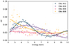 |
Fig. 9. Comparative PF spectra in the 2–11 keV band for the first four observations of Table 1. |
| In the text | |
|
Fig. 10. Pulsed fraction values (upper panel) and CC spectra (lower panel) for ObsID 802,804,806 and 808 in the 4–9 keV energy range. The position and width of the spectral emission iron line is marked by the dotted line and the purple-coloured area (1-sigma contour). |
| In the text | |
|
Fig. 11. Spectral characterisation of the phase-resolved peak excesses for ObsIDs 802, 804, 806, and 808. Each panel shows the photon excesses per energy bin for the blue (blue data) and the red peak (red data). The Gaussian best-fitting model for the red (blue) dataset is marked by a thick red (blue) line. |
| In the text | |
|
Fig. 12. Phase-resolved spectroscopy for ObsID 806. Left (Right) panel: phase-dependence of the red (blue) line normalisation (black dots in units of 10−4 photons/cm−2/s) superimposed with the energy-resolved pulse-profile (from Fig. 7). |
| In the text | |
|
Fig. 13. Phase-energy maps simulated from the solution of radiative transfer equation in a slab of highly magnetised plasma based on a model described by Sokolova-Lapa et al. (2023) and combined with relativistic ray tracing by Falkner (2018). A colour map shows the variation of a normalised total observed flux. The two maps are calculated for observer’s inclinations i and the same location of two identically emitting poles, specified by their polar angle from the spin axis Θ and their azimuthal separation ΔΦ (the values are indicated on the panels). For the geometry displayed on the left, phase shifts occur over a broad range around the line, being caused by the redistribution of photons in the wings. The blue wing is particularly strongly affected by the process due to relatively high electron temperature kT = 7 keV. |
| In the text | |
Current usage metrics show cumulative count of Article Views (full-text article views including HTML views, PDF and ePub downloads, according to the available data) and Abstracts Views on Vision4Press platform.
Data correspond to usage on the plateform after 2015. The current usage metrics is available 48-96 hours after online publication and is updated daily on week days.
Initial download of the metrics may take a while.