| Issue |
A&A
Volume 694, February 2025
|
|
|---|---|---|
| Article Number | A221 | |
| Number of page(s) | 13 | |
| Section | Numerical methods and codes | |
| DOI | https://doi.org/10.1051/0004-6361/202451280 | |
| Published online | 14 February 2025 | |
A new method for determining the onset times of solar energetic particles and their uncertainties: Poisson-CUSUM bootstrap hybrid method
1
Space Research Laboratory, Department of Physics and Astronomy,
20014 University of Turku,
Finland
2
Institut d’Estudis Espacials de Catalunya (IEEC), Edifici RDIT,
Campus UPC,
08860
Castelldefels (Barcelona),
Spain
3
Institute of Space Sciences (ICE, CSIC),
Campus UAB, Carrer de Can Magrans, s/n,
08193
Barcelona,
Spain
★ Corresponding author; This email address is being protected from spambots. You need JavaScript enabled to view it.
Received:
27
June
2024
Accepted:
10
January
2025
Abstract
Context. Solar energetic particle (SEP) events are a type of space weather phenomena in which highly energetic charged particles are released from the Sun into interplanetary space by violent and eruptive phenomena, such as solar flares and coronal mass ejections. In order to assess the origin of SEPs, an accurate timing of their arrival at spacecraft is of utmost importance. Several methods for determining the starting time of an SEP event at an observer exist, but the uncertainty of this starting time is not assessed in a systematic way by the vast majority of studies.
Aims. Employing a newly developed hybrid method of Poisson-CUSUM combined with bootstrapping, we show that the uncertainty related to the onset of an event in any particular energy range is often more than the mere time resolution of the measuring apparatus, and furthermore, it is not necessarily symmetric with respect to the past and future of the determined onset. In addition, we provide a software tool to the scientific community that applies the presented method and automates the determination of SEP event onset times and their related uncertainties, and it finally allows one to easily perform a velocity dispersion analysis.
Methods. By applying the Poisson-CUSUM method coupled with statistical bootstrapping to SEP event observations, we demonstrate the effectiveness of the method on synthetic and real data, and we compare them to an analysis conducted using a classical approach in which the uncertainty is assumed based on the time resolution of the data.
Results. In the example case, the inferred SEP path length and injection time related to the event, acquired by the velocity dispersion analysis, differ from what is obtained without properly assessing the uncertainty related to the onset times in varying energies. We also present the software package, PyOnset, that automates many steps of the method along with providing powerful data-visualization methods and analysis tools. We release the code to the scientific community as open-source software.
Key words: methods: data analysis / methods: observational / methods: statistical / Sun: particle emission
© The Authors 2025
 Open Access article, published by EDP Sciences, under the terms of the Creative Commons Attribution License (https://creativecommons.org/licenses/by/4.0), which permits unrestricted use, distribution, and reproduction in any medium, provided the original work is properly cited.
This article is published in open access under the Subscribe to Open model. This email address is being protected from spambots. You need JavaScript enabled to view it. to support open access publication.
1 Introduction
Solar energetic particles (SEPs) are charged particles that are accelerated to high energies in explosive phenomena, such as solar flares and shocks driven by coronal mass ejections (CMEs; see, e.g., Reames 2021, and references therein). They propagate through the interplanetary (IP) medium primarily along magnetic field lines. These particles pose a radiation hazard to electrical instrumentation and biological tissue on board of spacecraft (e.g., Vainio et al. 2009), and since reliable forecasting tools for SEP events are still lacking, it is very important to understand the acceleration and transport mechanisms of SEPs.
It is crucial to connect remote observations of eruptive phenomena that occur on the Sun to their in situ measurement counterparts in the IP space for relating the SEPs with their potential source regions and acceleration processes at the Sun. Therefore, one of the first steps in SEP analyses is to determine the event onset time at the observer in IP space. Traditional methods for determining these onset times have applied different types of algorithms, for example, plain threshold criteria such as a 3σ method (see, e.g., Krucker et al. 1999), fitting an exponential to the rising phase of the event (e.g., Dresing et al. 2012), and CUmulative SUM (CUSUM) methods such as Poisson- CUSUM. The different methods have their advantages and disadvantages, and known disadvantages of most of the methods used in the field are that especially with events that are characterized by a long and shallow rising phase they tend to find the onset time at a moment that is sometimes significantly later than what the human eye would deem as an appropriate onset time. Other major challenges to onset determination methods that can cause the found onset time to be delayed are low statistics and backgrounds that are characterized by high variability, high intensity, or residue from an earlier event (for reference see, e.g., Laitinen et al. 2010, 2015). Regardless, due to its versatility and usability, Poisson-CUSUM is widely used in the field of space physics when SEP event onset times are determined (see, e.g., Huttunen-Heikinmaa et al. 2005; Kouloumvakos et al. 2015; Paassilta et al. 2018; Ameri et al. 2019; Xu et al. 2020; Kollhoff et al. 2021).
The structure of this paper is as follows: we first introduce Poisson-CUSUM in detail. It is the central building block that our new hybrid method employs. We then describe the working principles of the new hybrid method with examples. We compare both synthetic data and an event that is analyzed using the traditional Poisson-CUSUM and our hybrid method, and we finally present the software tool that employs the hybrid method and automates many steps that any researcher needs to apply when analyzing any SEP event.
2 Methodology
The method presented in this paper finds the onset time of an SEP event and the uncertainty related to it using Poisson- CUSUM coupled with statistical bootstrapping and time averaging. Employing distributions of onset times acquired via bootstrapping from differently averaged data, this method finds the most probable onset time regardless of a subjectively chosen time resolution. The uncertainty related to this most probable onset time is evaluated using the widths of the onset distributions that come from differently time-averaged data. Each step of the method is described in detail in this section, and the list summarizing the main parts reads as follows:
Poisson-CUSUM deterministically finds one onset time that corresponds to a pair of pre-event background parameters (mean and standard deviation; Sect. 2).
A distribution of background parameter pairs is found by applying statistical bootstrapping to find a distribution of possible onset times (Sect. 2.1).
The data are resampled to a range of different time resolutions while the previous step is repeated (Sect. 2.2).
A positive time shift is applied to the time-averaged distributions to account for an increasing bin width. This artificially pushes the onset time backward in time (Sect. 2.3).
The weighted mean of the modes of all the distributions is calculated to acquire the most probable onset time (Sect. 2.4).
The CUSUM methods (Page 1954) are a set of quality-control schemes that in addition to having applications in time-series data analysis are also used in many industries to monitor the quality of manufactured products. When the monitored variable is expected to exhibit a Poisson distribution (which is typically the case for energetic particle measurements such as SEPs), the chosen CUSUM scheme is the Poisson-CUSUM (Lucas 1985). CUSUM methods are designed to give an early warning when the monitored variable either grows or shrinks too far from the acceptable range of values. In the case of SEPs, the monitored variable is either the count rate of particles or the physical unit of intensity that is calculated from particle counts and the geometric factor of the corresponding instrument. The acceptable range of values is defined by the mean and standard deviation of the intensity measurements in what is considered the pre-event background. The pre-event background time range from which the background parameters are calculated must be chosen manually by eye, and correct positioning of the background boundaries is imperative in finding an accurate onset time. Figure 1 shows the pre-event background and the onset of 85–105 keV electrons as seen by Solar Electron Proton Telescope (SEPT; Müller-Mellin et al. 2008) on board Solar Terrestrial Relations Observatory- A (STEREO; Kaiser 2005; Kaiser et al. 2008) associated with the widespread SEP event of April 17, 2021 (see, e.g., Dresing et al. 2023). The data in the figure were time-averaged to a three- minute resolution because the intensity data coupled with the gradual rising phase of the event vary strongly.
The onset time is identified from the time-series data by the Poisson-CUSUM method, which accumulates the values that noticeably differ from the event-preceding background. To calculate the CUSUM function, we used the z-standardized intensity Iz and a control parameter k, which were calculated such that
 (1)
(1)
 (2)
(2)
 (3)
(3)
where I is the intensity, µ and σ are the mean and standard deviation of the background intensity, n ∈ ℕ \{0} is a coefficient that was usually set to 2, and ln(⋅) is the natural logarithm. Furthermore, the control parameter k was rounded to the nearest integer value when k > 1. The CUSUM function S for each timestamp was then calculated as follows:
![Mathematical equation: $S\,[0] = 0,$](/articles/aa/full_html/2025/02/aa51280-24/aa51280-24-eq4.png) (4)
(4)
![Mathematical equation: $S\,[i] = \max \left( {0,{I_z}[i] - k + S[i - 1]} \right),$](/articles/aa/full_html/2025/02/aa51280-24/aa51280-24-eq5.png) (5)
(5)
where max(⋅,⋅) picks the larger of the two inputs. When the CUSUM function S exceeded a threshold value h, a warning signal was given. After a set number of consecutive warning signals, we were certain that the threshold was not exceeded because of a random fluctuation, but that the onset of the event was found. In this case, we backtracked to the first warning signal and identified that timestamp as the onset time. We followed the practice introduced by Huttunen-Heikinmaa et al. (2005) to set the hastiness threshold h = 1 when k ≤ 1, and h = 2 otherwise. No single objectively correct way exists to choose how many consecutive warning signals have to be counted before the onset time is identified since this can strongly depend on the data set that is used. However, most of the time, we favored using a number of data points corresponding to 30 minutes of threshold-exceeding counting rates or intensity, as also done by Huttunen-Heikinmaa et al. (2005) in their study, which employed energetic particle data from the High Energy Detector (HED) of the Energetic and Relativistic Nuclei and Electron experiment (ERNE; Torsti et al. 1995) on board the SOlar and Heliospheric Observatory (SOHO; Domingo et al. 1995). As another example of the Poisson-CUSUM method, Fig. 2 shows the onset determination using different time averages for ∼100 keV ions observed in the October 28, 2021 ground-level enhancement (GLE) SEP event (e.g., Papaioannou et al. 2022; Klein et al. 2022) as measured by the Electron Proton Telescope (EPT; Rodríguez-Pacheco et al. 2020) on board Solar Orbiter (Müller et al. 2020). Figure 2 illustrates the effect of onset times that are detected earlier as more time-averaging is applied, which arises because the time bins become wider and the statistics improve. There clearly is more to the uncertainty of the CUSUM method than the cadence of the measurement.
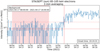 |
Fig. 1 Onset time of 85–105 keV electrons as observed by STEREO- A / SEPT found at 19:19:33 by traditional Poisson-CUSUM on the SEP event of April 17, 2021 with the background window set to 08:00–16:00 when using three-minute time-averaging. The onset time is marked with a vertical red line and the background window with light red. The mean of the background, µ, and µ + 2σ are illustrated with dashed and dotted red lines, respectively. |
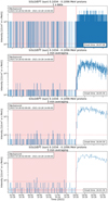 |
Fig. 2 Proton onset time of the October 28, 2021 (GLE73) event in the Solar Orbiter EPT (~100 keV) channel in 1 s, 1 min, 3 min, and 5 min time-averaging. The comparison shows that time-averaging the data affects the onset time determination with the Poisson-CUSUM method. |
2.1 A distribution of onset times
Since the CUSUM function only depends on the event background mean µ, standard deviation σ, and the chosen n, it deterministically maps a single pair of (µ, σ) to one and only one onset time in the time-series data. The common practice in the context of CUSUM methods is to consider all the data points in the background selection and find their mean and standard deviation. Our method, however, takes a more statistical perspective and chooses random samples from the population of data points inside the background window. While the random sampling can be mistaken for subsampling, which is a statistical method similar to bootstrapping, our method takes random samples from the background with replacement. This is done to produce a distribution of background parameter pairs (µ, σ) in order to map this distribution to a distribution of possible onset times. The idea as with the classic Poisson-CUSUM is that a single pair of (µ, σ) maps to a single onset time. After defining the background time window from which to take samples, our method takes random samples of size 0 < s < 1, where s is the fraction of data points taken from the background window for each sample. The method then calculates µ and σ for each of the samples. We then applied a bootstrapping approach. Let p ∈ ℕ be the number of samples taken. The method calculates p pairs of (µ, σ) and consequently finds p onset times that belong to the group of time stamps of the time-series data under analysis. Such a distribution with 1000 onset times is shown in Fig. 3 for STEREO-A / SEPT 85–105 keV electrons on the April 17, 2021 SEP event. A probability density representation of the same distribution is illustrated in Fig. 4, where the mode, the median, and the mean onset times of the distribution are marked with vertical lines. The red shading behind the histogram bars represents the middle ~68% interval of the distribution, that is, the moments of time that bound ~68% of the distribution, and the blue shading represents the middle ~95% of the distribution. Regardless of the three-minute integration time of the data in the distribution, the bins of the histogram have widths of one minute because the method randomizes the starting point of the time-series data within a single time bin. This procedure is further explained in detail in Sect. 2.1. The distribution exhibits a multimodal shape with three distinct local peaks. This is not strictly due to the three-minute integration time of the data, however, because multimodal onset time distributions can be seen in a variety of integration times. In this case, however, it is noteworthy to mention that the three peaks of the distribution are three, six, and nine minutes wide and are separated by valleys with widths of three and six minutes because of the three-minute integration time of the data. While it would be reasonable to assume that the shape of the distribution is caused by a time-dependent background, it is more related to the structure of the rising phase of the event in this integration time.
The statistical properties of this distribution of onset times are important in the context of our confidence of the onset time. The method presented in this paper uses the µ ± σ and µ ± 2σ per- centiles of the normal distribution as confidence intervals, which approximately correspond to the middle 68.27 and 95.45% of the respective distribution, regardless of the distribution shape. The exact shape and width of the resulting distribution always depends on the structure of the chosen background, however, on the rapidity of the rising part of the event, the choice for consecutive warning signals that one demands, and also the value of n in Eq. (2).
An event with a shape similar to the Heaviside function theoretically results in a distribution that approaches the Dirac delta function, almost regardless of the variability of the background. The reason is that the sudden intensity rise coming out of the background will, with any random sample from the background with some pair of (µ, σ), induce growth in the CUSUM function. On the other hand, the distribution shape in events with a very gradual rising phase depends much more strongly on the chosen background. The boundaries of the background selection should be chosen such that the intensity inside stays as constant as possible, that is, no large intensity increases or decreases are present. It should also be selected close to the onset of the event, and such that it encompasses as little residue from any potential earlier event as possible.
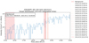 |
Fig. 3 85–105 keV electron intensity as observed by STEREO-A / SEPT during the widespread SEP event of April 17, 2021, averaged to a time resolution of 3 min. With 1000 bootstrap runs, each of which used a random sample size of 35% of the data inside the background, the method found a number of possible unique onset times that are displayed on the right of the figure with their respective distribution shares. The background window was set to 08:00–16:00 and is highlighted in light red. The most probable onset time (19:14:33) is marked with a vertical solid red line, while the rest of the onset times are marked with dashed lines. The depth of the color-shading indicates their relative popularity. |
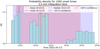 |
Fig. 4 Distribution of onset times produced by the method for STEREO-A / SEPT 85–105 keV electrons from the SEP event of April 17, 2021. These are the same spacecraft, instrument, particle species, energy range, and event as in Fig. 3. The mean, median, and mode of the distribution are marked with vertical orange, red and blue lines, respectively. The red shading behind the histogram shows the times that bound ~68% of the distribution, and the blue shading bounds ~95% of the distribution. |
2.2 Time-averaging of the data to obtain a set of onset-time distributions
The method presented here derives the most probable onset time, the median onset time, and two confidence intervals for an event using a set of onset-time distributions, with each of the distributions produced in the way described at the beginning of Sect. 2.1. The essential difference between these distributions is that they are drawn from data time-averaged to different, progressively lower resolutions.
The intensity time series exhibits irregular fluctuations or kinks that inhibit the Poisson-CUSUM method from finding the onset time in a reasonable range. It is therefore often helpful to average the data to a coarser time resolution in order to smooth out the information that is irrelevant to the larger-scale phenomenon of an SEP event and the time of its onset. By combining the onset-time distributions found in the same data as are averaged to different integration times, a better idea can be obtained whether Poisson-CUSUM accurately finds a good representative of the onset time in the original data that are in their native time resolution. Time-averaging also has the notable downside, however, that it decreases the intrinsic timing precision of the data, which provides the motivation to avert averaging the data more than is necessary.
After the distribution of onset times in the base cadence of the data1 is created, the method considers the width of that distribution and uses it as a basis to suggest a set T of distributions that are all time-averaged to different time resolutions, such that the maximum averaging time in the set is the width of the ~68% interval of the onset-time distribution of the original data. The first distribution of this set, T1, is that of the original intensity data with the native cadence. We therefore let  be the time stamp of the ith confidence interval (where ~68% is the first confidence interval and ~95% is the second) at its jth boundary, where i, j ∈ {1, 2} in the mth distribution of the set. The index m in practice corresponds to the time averaging of the data. For example, m = 1 corresponds to the data that were not time averaged, and m = 3 would correspond to the data that were time averaged to a three-minute resolution if the native data have a one-minute resolution. The method considers the first confidence interval of the distribution with the native cadence, that is,
  , and uses this as a suggestion to create the set of distributions with cardinality, that is, size,
  , where
  is an integer representation of
  rounded down to the nearest minute. This means that in practice, we used different time bin widths between the native cadence and the width of the ~68 % confidence interval obtained with the native cadence. Each distribution in the set comes from data that were time averaged to a progressively coarser time resolution in intervals of one minute and contains p onset times. The last distribution in the set,
  , comes from the data that were time averaged to a
  -minute time resolution. Each new distribution was created as described in Sect. 2.1, and the sample size s and the number of samples were taken p constant, while the time resolution of the data was progressively made coarser.
For longer integration times, the possible onset times occur in progressively coarser intervals, and they are dependent on the starting point of the time-averaging process. To take this into account, for every new time-series data with a cadence of m minutes in the set T, m − 1 copies of the time series are made, such that the averaging process for each of the copies started progressively one time step later from the start of the time series in one-minute intervals. In this way, the time-averaged time series and all its copies cover time stamps in a one-minute time resolution. This is illustrated in Fig. 5, which shows ten- minute averaged SOHO / ERNE (13–16 MeV) proton data and all their nine time-shifted copies, plotted over the original intensity data, which have a one-minute cadence. For each bootstrap run taking a random sample from a time series with a cadence m, the method also randomly selects either that time series or one of its time-shifted copies to seek the onset time from. The procedure thus essentially randomizes the starting point of the time-averaged data. This was again repeated p times and resulted in a distribution of p onset times that come from m versions of the same time-series data, each with a starting point one minute apart, but with the same time resolution.
A known caveat of building the set of distributions T using the width of the ~68% confidence interval  is that a potential kink in the intensity data, for example, a sudden drop in the intensity mid-onset, which for example arises because the spacecraft enters another interplanetary flux tube, may cause the CUSUM method to only find a very small number of unique onset times for a wide range of different (µ, σ) pairs. This falsely indicates great certainty in the onset time. This case is illustrated in Fig. 6 for a set of 20 onset-time distributions for STEREO /SEPT 55–65 keV electrons, where the native one-minute data resolution yields a distribution that disagrees significantly from the rest of the distributions in that the width of the distribution and its centering are noticeably different from any of the distributions obtained from time-averaged data. The figure shows the ~68 (purple) and ~95% (blue) intervals of the distributions as a function of data-integration time, as well as the mean, median, and mode of each distribution marked with an orange circle, red triangle, and blue pentagon, respectively. The horizontal lines also indicate the weighted mean of the median onset times (red) and the mean of the mode onset times (blue). The weighting was applied in accordance with the width of the ~95% interval of the distribution, such that small intervals receive a larger weight.
The distribution of the onset times occasionally has the shape of a delta function, that is, all p onset times are the same time, which would indicate  . This can clearly not be true because the differentiation capability of an instrument is limited. In these circumstances, and only then, the confidence are intervals automatically set to either the native data time resolution, or if time-averaging was applied to the integration time of the data, for the certainty that the onset time lies between times ti,1, ti,2, and the ith confidence interval may never be smaller than what the instrument is able to resolve, nor can it be zero. In general, the method does not allow for
  . If this situation were to occur, the time stamps
  would be moved away from their common midpoint by half of the integration time of their corresponding data because the minimum temporal uncertainty related to a measurement, even in the case of an event following an ideal Heaviside function, must be at least the integration time of the data. The integration time of the data, however, is a fundamentally different concept from some percentile of a bootstrapped distribution. They can therefore not be combined. One or the other has to be chosen as representative of the error.
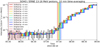 |
Fig. 5 SOHO / ERNE (13–16 MeV) protons in the August 18, 2010 SEP event. We superpose on the intensity data in native cadence (black curve) the ten-minute time-averaged version of the data along with their nine copies, which are all shifted forward in time in one-minute intervals (rainbow-colored curves). The onset found by Poisson-CUSUM for the native data is marked with a vertical black line, and the onsets found for the ten ten-minute data time series are marked with a vertical line whose colors correspond to the time series. |
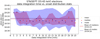 |
Fig. 6 Set of 20 distributions of electron onset times as a function of data integration time using STEREO-A / SEPT 55-65 keV electron data from the April 17, 2021 SEP event. Each distribution consists of 1000 possible onsets, and its mean, median, and mode are marked in the plot with a yellow circle, red triangle, and a blue pentagon, respectively. The purple and blue areas mark the times that bound ~68 and ~95% of the distribution. |
2.3 Detrending onset times
For the set of onset distributions based on different integration times, we applied a positive time shift to each onset time of half the integration time of the distribution +30 s. This positive time shift was applied to all but the native data in the set of distributions and is called detrending the distributions. The positive time shift was applied to correct the tendency of onset distributions to artificially shift to earlier times as the data integration time grows longer because the time bins become wider. The effect is illustrated in Fig. 2 for the case of a single onset time, where the onset time of ~100 keV ions measured by the Solar Orbiter EPT is seen to shift to earlier times as longer time-averaging is applied to the intensity data. Even after the time-averaging, the time assigned to an intensity bin is still in the middle of the time interval, and the tendency of the onset times to shift to earlier times as time-averaging is applied is therefore not due to a native time-averaging process, which would not take the shifting of the time stamp to the middle of the time interval after the averaging into account. The cause instead is the widening of the data bins, which cause the high intensity of the event to be apparent earlier. The effect of detrending entire distributions is shown in Fig. 7, where we compare a set of distributions without detrending (lower panel) and a set of distributions with detrending (upper panel). The ~68 (purple) and ~95 (blue) distribution percentiles have a downward trend in the lower panel, which is corrected for in the upper panel of the figure.
2.4 Determining the final onset time and its uncertainty
A traditional way to estimate the uncertainty of the onset time has been to use the time resolution of the data as the confidence interval, centered at the onset time. The certainty in this confidence interval is usually not specified either, which in principle either implies a 100% confidence that the onset time is at some time t ± Δu/2, or that we have no knowledge of our confidence of the interval.
In order to assess the most probable onset time and its confidence intervals, we used the set of onset-time distributions T that our method produced. Each distribution provides one most frequent onset time, which is the mode of the distribution. For each integration time, there exists a distribution in the set that reflects the most probable onset time and its uncertainty in that integration time. Taking a weighted mean of these modes yields an onset time that is closest to any onset time that would be obtained regardless of the sample that is taken from the background window or data-integration time. We call this the most probable onset time.
The method calculated individual weighted means of the timestamps for the mode, median, and confidence interval bounds of the onset times. In order to prioritize the distributions with greater precision, the method applied weights in the calculation of the averages. We used the statistic inverse-variance weighting method (e.g., Hartung et al. 2008) to calculate the means of the time stamps. With inverse-variance weighting, the individual time stamps were weighted in proportion to the inverse of the variance of the distribution to which the time stamp belongs. In this way, we favored the narrower distributions, that is, those that represent a more precise measurement.
It is also possible, and in some cases even necessary, to set the averaging of the time series to reach a specific time resolution instead of letting the method decide it for the user. In other words, to deliberately make n distributions even though the ~68% confidence interval might be a number smaller than n. This is especially the case when the ~68% confidence interval of the native nonaveraged data is very small for an event that is clearly gradual in its nature. This is illustrated in Fig. 6 for the STEREO-A / SEPT (55–65 keV) electron onset-time distribution in the native time resolution  min, but further time averaging revealed that the data did not necessarily accurately represent the onset time and its uncertainty.
After the weighting was applied on all time stamps of the set of distributions, six time stamps remained that characterize the result: mode, median, ~68% lower bound, ~68% higher bound, ~95% lower bound, and ~95% higher bound. Whether the weighted mode or the median is deemed more appropriate to represent the onset time, it is noteworthy to mention that the resulting error bars are not necessarily symmetric around the onset time, in contrast to traditional practice.
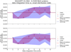 |
Fig. 7 Comparison of a set of Solar Orbiter / EPT ~245 keV ion onset-time distributions for the October 28, 2021 GLE event as a function of data-integration time. The upper panel displays the distributions with detrending, and the lower panel shows this without detrending. For this run, the native data time resolution was skipped because it was very different from the distributions produced by time-averaged data, and one-minute data were used instead. For the one-minute data, |

3 Comparison of results: Traditional Poisson-CUSUM versus the Poisson-CUSUM bootstrap hybrid method
The traditional way of finding an onset time with Poisson- CUSUM is to take the mean and standard deviation of the pre-event background (µ, σ) and calculate the control parameter k that restricts the growth of the CUSUM function. The point at which CUSUM exceeds h and stays above it for a specified amount of time is the time when the onset of the event is identified.
The Poisson-CUSUM bootstrap hybrid method takes the statistical perspective to find the onset time. Instead of finding the mean and standard deviation of the whole pre-event background, our method takes random samples from the pre-event background and finds a distribution of possible onset times. Using the width of the ~68% interval of this distribution, the method suggests a suitable maximum data-averaging time and creates a new distribution of onset times for each consecutive averaging time from the native cadence up to the suggested maximum data-averaging time.
To demonstrate the new hybrid method, we prepared three synthetic events (from now on referred to as E1, E2, and E3) with distinct characteristics. E1 represents an event with a rapid rising phase with a rise-time Δt ≈ 30 min and a static background. This combination is expected to yield a nearly unambiguous onset time right at the foot of the rising phase. E2 models a gradual rising phase also with a static background, with Δt between the onset and the peak being over six hours. This type of event is expected to have a larger uncertainty in the onset time, which often required some time-averaging with the classical Poisson- CUSUM. E3 represents an event that is otherwise identical to E2, but has a dynamic background. The three synthetic time-series with the found onset times are displayed in Fig. 8.
To prepare the synthetic event profiles, we used an empirical functional form of the count rate,
![Mathematical equation: $N\left( {t;{t_0},a,b,c} \right) = {a \over {{{\left[ {bc\left( {t - {t_0}} \right)} \right]}^c}}}\exp \left\{ {c - {1 \over {b\left( {t - {t_0}} \right)}}} \right\},\quad t > {t_0},$](/articles/aa/full_html/2025/02/aa51280-24/aa51280-24-eq19.png)
motivated by the solution of the diffusion equation (see Wang et al. 2022). The function has four parameters: t0, a, b, and c. For all three events, the parameter a that controls the peak height of the profile was set to a = 100 and t0, which defines the onset time, was (arbitrarily) set to t0 = 02:00:00 on January 3, 1900. The date and time here do no correspond to any real event or data, but were chosen for a period of time that is commonly known to have no in situ space observations. As the PyOnset (see Appendix A) software works with time-series data, some time stamps had to be generated for the artificial data points. The onset time t0 set in the event profile does not correspond to the observed onset time of the event because the profile takes a finite time depending on the rise phase to increase above the background. This was set for all events set to µ = 1. For the rapid event E1, the parameters b and c that control the rise and decay of the profile were set to b = 0.01 min−1 and c = 0.5, which produced the time of maximum of tmax − t0 = 1/(bc) = 200 min, that is, a rapid onset. The event profiles for E2 and E3 are identical. For both of them, b = 0.003 min−1 and c = 0.001, resulting in a much more gradual rising phase followed by a plateau, which could represent an SEP event caused by a propagating interplanetary shock. The background for E1 and E2 was set to a static value µ = 1, while for E3, we created a dynamic background that followed a sinusoidal with a period of six hours and an amplitude of 0.5 times the background mean of µ = 1. The dynamic background was intended to emulate slow changes in the particle intensity that are often observed in real data. Finally, for all events, the synthetic counting rates were generated with the created profiles using the Poisson random generator of NumPy (Harris et al. 2020).
To determine the onset time for each of the events with the two methods, the background window from which we extracted the CUSUM parameters was set to 03:00 on January 1−22:00 on January 2, so that it was extensive while still not extending too close to the events. Figure 8 shows the possible onset times found by the hybrid method drawn over the time series of the three events in base cadence, which is one minute. For the hybrid method, we used a sample size of s = 35% for the bootstrapping with p = 1000 samples. The most probable onset time in base cadence also corresponds to the onset time found by the traditional Poisson-CUSUM, which is an expected result. Since the hybrid method found a distribution of possible onset times for each of the synthetic events, it also applied time averaging to the data and found new distributions of possible onset times from the time-averaged versions of the data. Finally, the hybrid method calculated the weighted mean of the modes of the distributions, resulting in the most probable onset time for each event. The results are presented in Table 1. The hybrid method finds the onset time slightly earlier in these events than the classical Poisson-CUSUM, and the hybrid method also yields much larger and nonsymmetrical uncertainties for the onset times. In general, a larger and nonsymmetric uncertainty is more realistic in the context of SEP event onset times.
In addition to the synthetic data, we also ran the Poisson- CUSUM bootstrap hybrid method on the proton data of SOHO/ERNE for an SEP event that occurred on November 22, 1998, and we compared the results to those of the traditional Poisson-CUSUM with an identical background choice. This event was reported in the first SEPserver event catalog (Vainio et al. 2013), where the authors performed a velocity dispersion analysis (VDA; e.g., Lintunen & Vainio 2004) on the onset times observed by SOHO/ERNE. The authors of the catalog reported that a fit to all 20 energy channels of ERNE yielded a path length L = 1.51 ± 0.09 AU and an injection time tinj = 06:43±0:06:00. The X4 class flare that was associated with the event was located on 82W longitude (in Stonyhurst coordinates) and started at 06:30. It is reasonable to assume that the magnetic connection between the source of acceleration and SOHO was probably good. This is because neither the calculated path length deviates drastically from a nominal Parker spiral arc length at 1 AU, nor does the inferred injection time from the timing of the associated flare. Under ideal conditions, the L1 point is known to be well magnetically connected to the western side of the solar limb. For this reason, and because all energy channels were used for VDA, this is a good candidate for a comparison.
For this event, we set the background to 00:00−07:15 on November 22, 1998, and the number of bootstrap runs for the hybrid method was set to p = 1000. We note that the background we used here is not necessarily the same as in Vainio et al. (2013) because they did not report what type of background selection they used. The sample size for the hybrid method was set to 45%, and since the length of the background is 435 minutes, we limited the hybrid method to average the data to four minutes at most to preserve at least 100 data points in the background selection. The original data have a time resolution of one minute, so they were not time averaged or altered in any other way. Figure 9 shows a comparison between the onset times found by the Poisson-CUSUM-bootstrap hybrid method presented in this paper (green and blue markers) and the classical Poisson- CUSUM (red markers). In the figure, the horizontal error bars display the widths of the respective energy channels, with the data point placed at the geometric mean of the channel boundaries. The vertical error bars show the 95% confidence intervals related to each onset time found by the hybrid method, which are also listed in Tables B.1 (blue markers, ERNE-LED) and B.2 (green markers, ERNE-HED). For the red markers, no horizontal errors were plotted because they are identical to the green and blue markers, but the vertical errors, which are a constant ±30 s for the width of the one-minute time bin, were plotted.
The two methods finds similar onset times, and the onset times show a clear trend of the onset occurring earlier as the proton energy grows higher, that is, the 1/β decreases. The energy regime where velocity dispersion is not observed lies between 2 ≤ 1/β ≤ 4, which in Fig. 9 is shown as the onset time found by both of the methods being close to a constant despite changing 1/β. Moreover, for the 100–130 MeV channel (index 9) of ERNE-HED (High Energy Detector), no onset was found by either method due to a lack of any notable increase in particle intensity, even though Vainio et al. (2013) acquired an onset time, albeit a very late one (07:48 UT). An onset time was found for every energy channel on ERNE-LED (Low Energy Detector). As previously stated, a comparison of all the onset times found by both methods and the related uncertainties is summarized in Tables B.1 and B.2. For many of the energy channels, the hybrid method and the classical Poisson-CUSUM agree on the onset times with an identical background choice. This is expected since the event has a very clear profile in every energy channel that exhibits an intensity rise that can be caught by Poisson- CUSUM. Most of the onset times found by the hybrid method are also rather precise and have relatively small uncertainties. The one major exception is the 1.5–1.8 MeV channel (index 0) of ERNE-LED, where the hybrid method finds an onset time at 10:15:39, 28 seconds earlier than the classical Poisson-CUSUM, but with a large uncertainty. The cause of this large uncertainty is the low background level of the channel, which has ample zero-count measurements in the background interval. Applying the Poisson-CUSUM method to this background usually leads to an early and abrupt detection of the onset upon an even slight intensity enhancement. With the hybrid method, it leads to background samples that have many zeros in them, causing a number of possible onsets to be found very early in relation to the actual strong increase in intensity. The time error of this onset time is therefore strongly asymmetric, and the most probable onset time is found near the end of the 95% confidence interval.
The VDA fit applied to the onset times found by the hybrid method and the time applied to the onset times found by the classical Poisson-CUSUM produce reasonable and rather similar results. The linear fit shown in Fig. 9 is the fit applied to the onset times found by the hybrid method, and it yields a path length L = 1.600 ± 0.145 AU and an injection time tinj = 06:38 ± 0:08:33. A fit applied to the onset times found by the classical Poisson-CUSUM (red markers in Fig. 9) yields a path length L = 1.558 ± 0.106 AU and an injection time tinj = 06:41 ± 0:07:51. The two fits agree well with the results of Vainio et al. (2013) within the margin of error, although the fit applied to onset times found by the hybrid method is the only fit that takes errors into account that are systematically evaluated.
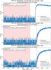 |
Fig. 8 Three simulated SEP events and the onset analysis results of the hybrid method for the base cadence (one minute). The most probable onset time in base cadence (solid vertical red line) in each panel is also the onset time found by the classical Poisson-CUSUM. |
Onset-time results of the three simulated SEP events calculated by the hybrid method and classical Poisson-CUSUM.
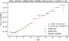 |
Fig. 9 Comparison between the energy-dependent onset times of the November 22, 1998 SEP event observed by SOHO/ERNE found by the Poisson-CUSUM bootstrap hybrid method (blue and green) and the classical Poisson-CUSUM (red). The vertical axis marks the onset time, and the horizontal axis, 1/β = c/v, is the inverse unitless speed of the protons. The horizontal error bars represent the widths of the ERNE proton energy channels, and the vertical error bars represent the uncertainty in time, which is the ~95% confidence interval for the hybrid method. For the red onset times, the horizontal error is not plotted because it is identical to the green and blue data points, but the vertical error bars (±30 s = data time resolution) are shown. The velocity dispersion analysis applied on the onset times found by the hybrid method using orthogonal distance regression yields a path length of 1.6 AU and an injection time of 06:38. |
4 Discussion
The primary motivation for developing the method presented in this paper was that the uncertainty of the onset time of an SEP event was not considered by traditional methods. Instead, the integration time of the data is usually reported as the uncertainty. This is a problem for two reasons. First, the choice of which integration time to use, that is, how much the data are time averaged, introduces subjectivity into the onset time itself and its apparent uncertainty. Second, there is no reason to assume that the uncertainty of an onset time should necessarily be symmetric with regard to the past and future of the onset time, and that this uncertainty would be exactly the width of the time bin that is used at the time. The method presented in this paper aims to reduce the subjectivity related to the onset time itself and its uncertainty by introducing a systematic process to evaluate them.
The three synthetic example cases that were shown and analyzed in Sect. 3 represent idealized versions of three types of SEP events that are often encountered when studying SEP events. E1 is an event with a static background and a short rising phase, which makes its onset time easy to identify in most cases. E2 and E3 are both events with a slow rising phase, and the exact moment when the event starts therefore becomes more ambiguous. As we discussed in Sect. 2, for an idealized event with the shape of a Heaviside function, the uncertainty of an onset time should theoretically be a symmetric time interval with the length of the integration time of the data. This is because at the start of the idealized event, the ith measurement belongs to the background, while the (i + 1)th measurement is at the peak intensity level. Hence, the onset of the event must be found at the (i + 1)th measurement, regardless of the random sample taken from the pre-event background, which is static. Since an instrument with a finite cadence has taken the measurements, the event may have begun at any moment of time within the (i + 1)th bin. Thus, in the idealized case where the SEP event has the shape of a Heaviside function, the uncertainty related to the onset time is the integration time of the data. We expect that as the profile of an SEP event deviates from an idealized event profile, the uncertainty related to the onset time increases. It is reasonable to assume that the shape of the event profile may also introduce an asymmetry in the uncertainty.
The simulated event E1 represents a relatively rapid event with a short rising phase and a steep rise from the background level to the intensity peak. In terms of the events studied by Wang et al. (2022), E1 is one of the fastest to rise from onset to peak for 20–25 MeV protons. Despite its short rise-time and steep rise, it is still not quite an ideal Heaviside function-like event, since the rise from background level to the peak is not an instantaneous step. The hybrid method finds two plausible onset times in the base cadence for this event, 02:14 and 02:18, and one very unlikely time, 02:17. The most probable onset time in base cadence, 02:18, is also the time that the traditional Poisson-CUSUM finds as the onset time, which is expected. In general, we expect that most of the bootstrap samples taken from the pre-event background selection exhibit attributes that closely resemble the attributes of the entire background selection. Since the distribution of onset times in base cadence has a width of four minutes, time averaging up to four minutes was applied to the data and the procedure was repeated. The method found that the most probable onset time for data with a one-, two-, three-, and four-minute resolution is 02:16:56, and the uncertainty increases more toward the background (past) of the onset than toward the event (future). This is expected because just a single measurement that surpasses the k-parameter defined in Eq. (3) by the value of h at least (the hastiness threshold) at the foot of the event may trigger Poisson-CUSUM, resulting in a slightly earlier onset time. Events E2 and E3 both represent an event with a slow and gradual rise. The rise time of their event profiles is extremely long and mimics a slow rise with continuous injection, for example. Because the measurements fluctuate, we expect in general that as the rising phase of an event profile becomes shallower, the uncertainty related to the onset time increases. The same applies to variable background intensity levels because they can either mask or incorrectly amplify the apparent rising phase of an event. The time-dependent sinusoidal background in E3 is thought to mimic a changing background-intensity level, which can make it more difficult to identify the onset time of an event for the reasons described above. In the case of E3, the bootstrapping part of the hybrid method produces a wider distribution of (μ, σ) pairs (because a more diverse population of data points exist from which random samples can be taken), which in turn leads to a wider distribution of possible onset times. This has the desired effect of the method evaluating the uncertainty of the onset of an event such as E3 to be higher than an event with a static and stable pre-event background. In general, the uncertainty of an onset time is always dependent on the combination of at least the processes discussed above, the signal-to-noise ratio of the measurements, how gradual the rise is, and how variable the pre-event background is (Laitinen et al. 2010, 2015).
5 Concluding remarks
We have introduced and described in detail the new method for determining the onset times of SEP events by applying the established Poisson-CUSUM method in concert with statistical bootstrapping. This method is the first to provide reasonable, consistent, and objective uncertainties related to the onset times of SEP events in a systematic way. The VDA applied to the onset times acquired with this method are therefore more physically meaningful. In addition, one of the biggest strengths of the new method is that it is very general in its nature, so that it can also be applied to a variety of time series data that are Poisson-distributed.
From a mathematical point of view, the mean of the background period can also be interpreted as the expected value of the background. Since the hybrid method presented in this paper operates by taking random samples from the background, the expected value of these random samples should remain close to the mean of the entire background period as long as the samples are large enough to be representative of the entire background period. Hence, it is expected that under perfect conditions, where the data are produced by a stable Poissonian process, the hybrid method will find the most probable onset time with any integration time to be the same as what classical Poisson-CUSUM does with the same integration time while also providing a more reasonable uncertainty.
However, it is the conditions of the solar wind, including but not limited to magnetic structures and pitch angle changes, that are able to break the assumption that the error of measurement is purely related to counting statistics, and they therefore introduce additional uncertainty in the onset time of an SEP event. These dynamic changes in the background in particular enable the hybrid method to find more than one possible onset time for an SEP event.
We note that real SEP data may deviate from the ideal data produced by a pure and steady Poissonian process for the aforementioned reasons. As long as this deviation is not extreme, the method is expected to be viable for application to the data. In an extreme case where the data are not representative of the counting rate statistics, neither this method nor Poisson-CUSUM should be applied in hopes of finding reliable onset times. Data like this are, for example, data that are produced by difference imaging. This is because difference imaging may apply a nonuniform subtraction to the data, and this process transforms data into something that cannot be replicated by a stable Poissonian process.
The software package PyOnset, introduced in Appendix A and released to the scientific community along with this paper being publicly available on Github2, provides a practical and convenient way to apply the hybrid method to SEP events, while also preserving the ability to use the classical Poisson-CUSUM for quick-look onset times without uncertainty. Pyonset was used to create all of the figures or their layouts in this paper, and it is open-source Python software released under the BSD-3-Clause license.
Acknowledgements
We acknowledge funding by the European Union’s Horizon 2020 / Horizon Europe research and innovation programmes under grant agreements No. 101004159 (SERPENTINE) and No. 101134999 (SOLER). N.D. is grateful for support by the Research Council of Finland (SHOCKSEE, grant No. 346902). The research is performed under the umbrella of the Finnish Centre of Excellence in Research of Sustainable Space (FORESAIL). C.P.G. acknowledges financial support from the Secretary of Universities and Research (Government of Catalonia) and by the Horizon 2020 Research and Innovation Programme of the European Union under the Marie Skłodowska-Curie and the Beatriu de Pinós 2021 BP 00168 programme, from the Spanish Ministerio de Ciencia e Innovación (MCIN) and the Agencia Estatal de Investigación (AEI) 10.13039/501100011033 under the PID2020-115253GA-I00 HOSTFLOWS project, and the program Unidad de Excelencia María de Maeztu CEX2020-001058-M.
Appendix A Software: PyOnset
Using the SEPpy software package developed by Palmroos et al. (2022) as a base to build on, we have created a semi-automated workflow that employs our newly developed method to assess the onset time and its uncertainty of an SEP event. The software, called PyOnset, comes in a Python package, which is also possible to conveniently be run from a Jupyter Notebook (Jupyter: Kluyver et al. 2016).
The package inherits the functionality of SEPpy, including various data loaders for spacecraft-based energetic particle data, as well as an onset determination using the traditional Poisson-CUSUM method. The new package is fully backwards- compatible and extends its scope of usability to apply our new onset-determination hybrid method. PyOnset includes visualizing the many aspects of the statistics produced by the method, and using the uncertainty of an onset in varying energy channels to conduct higher-level analyses, such as velocity dispersion analysis.
The software is structured such that it employs three different objects to carry out the determination of the onset time and uncertainty related to it, to produce a variety of plots to visualize the different distributions of possible onset times and to apply VDA to the found onset times. These objects are called Onset, BootstrapWindow and OnsetStatsArray, and they will be individually introduced in Appendices A.1 (Onset), A.2 (BootstrapWindow), and A.3 (OnsetStatsArray). Onset and BootstrapWindow are objects that are indispensable to finding the onset times and their uncertainties, while the OnsetStatsArray object is used for storing the different distributions of onset times that are produced while applying different time-averagings to the data, and to visualize these distributions and their statistics.
The standard workflow with the software starts with initializing an Onset object with a given spacecraft , sensor, particle species (electron, ion, proton) and a viewing that is the viewing direction of the sensor. By providing a range of dates to the Onset object, the data loaders of SEPpy automatically fetch the data either from a local directory or from the internet and save it to a Pandas DataFrame object in the Onset object’s memory.
After an Onset object is initialized, the first analysis step is to identify the event. Therefore, a simple quick-look onset determination is run on the dataset. Based on the resulting plot, the user then chooses a reasonable background interval, which is set to BootstrapWindow. This step is often an iterative process because one rarely identifies the optimal background window on the first try. Furthermore, if the user should intend to find the onset time on multiple energy channels, they must make sure that the background window does not overlap with the start of the event in any of the chosen energy channels. If this is not done, it may cause onset times "flatlining", meaning that the onset time beyond some energy is found at the exact same moment of time in all energies, which is the end of the background window, effectively making velocity dispersion analysis impossible.
Once the background window is reasonably defined, the onset time and accompanying uncertainties can be found using the onset_statistics_per_channel()-method of the Onset object. This method must be provided with a BootstrapWindow object so that the background window and the amount of bootstrapped random samples are known. It also requires an input for the keyword channels, which controls which channels to run the method on. By default, onset_statistics_per_channel() time-averages the data up to the width of the ∼68 % confidence interval, albeit it is also possible to choose by hand the maximum data averaging time, in which case the software will ignore the suggestion given by  and create a set of as many distributions as requested. Such is the case in Fig. 6, where
  .
.
A.1 The Onset object
Onset is the primary tool for finding the onset time in any available energy channel of the chosen spacecraft+instrument combination. The most fundamental method of this object is the cusum_onset(), which is the starting point of any SEP event analysis. cusum_onset() finds an onset time using the Poisson-CUSUM method given a background window, that is provided as a BootstrapWindow object. The point of running cusum_onset() is to find, by eye, a reasonable background window that yields an onset time for the event. This will produce a figure like Fig. 1, and simultaneously yield an onset time for the chosen channel with the classic Poisson-CUSUM method. It is also recommended to check for multiple energy channels so that the set background window does not overlap with the start of the event in any of the energy channels, to avert finding an onset time on an erroneous moment in time. The cusum_onset() method also has a diagnostics mode that is enabled by passing the argument diagnostics=True, that produces a figure like Fig. A.2, where the user can see at which point the CUSUM function starts to produce warning signals and how the choice of n affects this.
The onset_statistics_per_channel() method runs the statistical process described in Sect. 2 of finding the most probable onset time, the mean of the medians of onset times, and the ∼68 % and ∼95 % confidence intervals for all the selected energy channels. It is possible to run the method for just a single channel by giving the method parameter channels as a single integer number, or to a list of channels by providing an array-like object such as a tuple, list or a numpy array of integer numbers. It is also possible to run the method for all channels available to the chosen instrument by simply setting channels="all". The same background window is used for all the channels that are handled by the method, and the user is able to control the sample size of each bootstrap run with the parameter sample_size, which is by default set to 0.5 if no value is provided. Running the onset_statistics_per_channel() returns a list of OnsetStatsArray objects, where each of the objects in the list contains all the distributions that were produced to find the most probable onset time and the two confidence intervals of that energy channel. These distributions and their specific characteristics are not needed for any further calculations; rather they exist merely for visualization purposes. In fact, all the necessary information regarding an onset time at a particular energy and its uncertainty is stored in the Onset object itself, in a dictionary called "onset_statistics".
If an onset time and the accompanying uncertainties have been found using the onset_statistics_per_channel() method, one can run the VDA() method that automatically receives the energy-dependent onset times from the Onset object’s memory and applies a fit to those onset times as a function of the inverse unitless speed (β−1 = c/v, where c is the speed of light and v is the speed of the particle as calculated from the mean energy of the channel). The method uses a selection of energy channels, provided either as a Python slice or as a boolean list to the optional keyword parameter selection, and applies an orthogonal distance regression algorithm (ODR) to fit a first order polynomial to the onset times. Figure 9 shows VDAs applied to the ion onset times of Solar Orbiter/EPT of the 2023-03-13 SEP event, where in the top plot the onset times and their error bars are found using our new hybrid method using PyOnset, while in the bottom plot the onset times are found by the traditional Poisson-CUSUM method. The individual onset times acquired by the traditional Poisson-CUSUM and the hybrid method presented in this paper are included in Table B.1. The slope of the polynomial fit represents the path length L that the particles traveled and the intersection with the y-axis is the common solar injection time of the particles. The VDA() method plots the onset times and the linear fit as a function of the inverse unitless speed, and also returns a Python dictionary that holds the onset times of all energy channels and their error bars, their corresponding inverse betas and their error bars, the uncertainties related to the path length and the injection time resulting from the fit, the figure object and its axes, and the residual variance and stopping reason of the ODR algorithm.
A.2 The BootstrapWindow object
A BootstrapWindow object defines the start and end of the pre-event background. It also controls the amount of bootstrapped random samples that the method extracts from the background. It takes as an input three parameters: start, end and bootstraps.
start: A pandas-compatible datetime string, for example, "2023-12-30 12:00:00," that defines the starting point of the background.
end: A pandas-compatible datetime string, for example, "2023-12-31 12:00:00," that defines the ending point of the background.
bootstraps: An integer value that defines the number of samples that the method onset_statistics_per_channel() will produce when determining the onset time and its uncertainty. The default amount of bootstraps is 1, which means that if not specified otherwise, the methods of Onset will only seek for a single onset time, effectively working as the classical Poisson-CUSUM.
This object also has a method called print_max_recommended_reso() that prints out the maximum recommended time-averaging yielding at least a hundred data points to pick from inside the background window. This method can be run on its own at any point after the object is initialized with start and end, but it is also run inside the Onset object’s method onset_statistics_per_channel() if one enables printing of information by setting the parameter print_output=True.
A.3 OnsetStatsArray
As the name implies, OnsetStatsArray is an array of "statistics", where data from each individual distribution that is used to estimate the onset time and its uncertainty is stored in a dictionary that holds all the unique onset times and statistics related to a distribution collected from a time series that has a specific time averaging applied to it. The structure of an OnsetStatsArray is such that a single object holds all the different time-averaging statistics for a single energy channel in an attribute called archive. The archive is a list of dictionaries, where each dictionary includes the mean, median, mode, ∼68 %, and ∼95 % confidence intervals for a distribution of onset times in varying integration times. The object also has methods to visualize the onset time distributions and the attributes of the distributions.
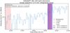 |
Fig. A.1 Distribution statistics for the 3-minute time-averaged data of STEREO-A / SEPT 85–105 keV electrons on the 2021-04-17 SEP event. The corresponding onset times are displayed on top of the time series in Fig. 3 and as a histogram in Fig. 4. The figure here shows the median (red), mode (blue) and the mean (orange) of the distribution as vertical lines and the ∼68 % (purple) and ∼95 % (blue) confidence intervals of the distribution as shadings. The chosen background for the method is seen on the left of the figure as light red shading. |
show_onset_distribution() is a method of OnsetStatsArray that displays the distribution of onset times at a given integration time marked on the time series data. The parameter integration_time_index is by default 0, which corresponds to no time-averaging applied (T1 in the set of onset time distributions), and can be changed to display the distribution of any time-averaged data. Figure 3 was produced with this method.
show_onset_statistics() is a method that displays the median, mode, mean, ∼68 % and ∼95 % percentiles at the given integration time drawn over the time series data. In the same fashion as for show_onset_distribution(), this method also defaults to showing the statistics of the native data resolution but can display other distribution’s statistics by changing the parameter integration_time_index. An example case for figures that this method produces is shown in Fig. A.1.
onset_time_histogram() is a method that displays the distribution of onset times as a probability distribution histogram. A figure like this is shown in Fig. 4.
integration_time_plot() is a method that produces a figure such as Fig. 6, where the onset time distribution attributes are displayed as a function of data integration time.
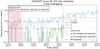 |
Fig. A.2 Onset diagnostics for the 3-minute time-averaged data of STEREO-A / SEPT 85–105 keV electrons on the 2021-04-17 SEP event. The corresponding onset time plot is displayed in Fig. 1. The figure shows the CUSUM function (dark red curve) along with its arguments: z-standardized intensity (green), k (dashed black line), and h (dash- dotted black line). The figure also shows, just like the standard plot without diagnostics, the mean of the background (horizontal dashed red line) and the µ + nσ line, where n = 2 (horizontal dotted red line). |
Appendix B Onset time comparison tables
The onset time comparison tables present the onset times found by the Poisson-CUSUM-bootstrap hybrid method introduced in this paper and the classical Poisson-CUSUM for the 199811-22 SEP event as measured by ERNE-LED (Table B.1) and ERNE-HED (B.2) aboard the SOHO spacecraft. The onset time comparison is visualized in Fig. 9.
Comparison of onset times found by the hybrid method and simple Poisson-CUSUM for SOHO/ERNE-LED observations on 199811-22.
Comparison of onset times found by the hybrid method and simple Poisson-CUSUM for SOHO/ERNE-HED observations on 1998-11-22.
References
- Ameri, D., Valtonen, E., & Pohjolainen, S. 2019, Sol. Phys., 294, 183 [NASA ADS] [CrossRef] [Google Scholar]
- Domingo, V., Fleck, B., & Poland, A. I. 1995, Sol. Phys., 162, 1 [Google Scholar]
- Dresing, N., Gómez-Herrero, R., Klassen, A., et al. 2012, Sol. Phys., 281, 281 [NASA ADS] [Google Scholar]
- Dresing, N., Rodríguez-García, L., Jebaraj, I. C., et al. 2023, A&A, 674, A105 [NASA ADS] [CrossRef] [EDP Sciences] [Google Scholar]
- Harris, C. R., Millman, K. J., van der Walt, S. J., et al. 2020, Nature, 585, 357 [NASA ADS] [CrossRef] [Google Scholar]
- Hartung, J., Knapp, G., & Sinha, B. 2008, Statistical Meta-Analysis with Applications, Wiley Series in Probability and Statistics (Hoboken: Wiley) [CrossRef] [Google Scholar]
- Huttunen-Heikinmaa, K., Valtonen, E., & Laitinen, T. 2005, A&A, 442, 673 [NASA ADS] [CrossRef] [EDP Sciences] [Google Scholar]
- Kaiser, M. L. 2005, Adv. Space Res., 36, 1483 [NASA ADS] [CrossRef] [Google Scholar]
- Kaiser, M. L., Kucera, T. A., Davila, J. M., et al. 2008, Space Sci. Rev., 136, 5 [Google Scholar]
- Klein, K.-L., Musset, S., Vilmer, N., et al. 2022, A&A, 663, A173 [CrossRef] [EDP Sciences] [Google Scholar]
- Kluyver, T., Ragan-Kelley, B., Pérez, F., et al. 2016, in Positioning and Power in Academic Publishing: Players, Agents and Agendas (Amsterdam: IOS Press), 87 [Google Scholar]
- Kollhoff, Kouloumvakos, A., Lario, D., et al. 2021, A&A, 656, A20 [NASA ADS] [CrossRef] [EDP Sciences] [Google Scholar]
- Kouloumvakos, A., Nindos, A., Valtonen, E., et al. 2015, A&A, 580, A80 [NASA ADS] [CrossRef] [EDP Sciences] [Google Scholar]
- Krucker, S., Larson, D. E., Lin, R. P., & Thompson, B. J. 1999, ApJ, 519, 864 [CrossRef] [Google Scholar]
- Laitinen, T., Huttunen-Heikinmaa, K., & Valtonen, E. 2010, AIP Conf. Proc., 1216, 249 [NASA ADS] [CrossRef] [Google Scholar]
- Laitinen, T., Huttunen-Heikinmaa, K., Valtonen, E., & Dalla, S. 2015, ApJ, 806, 114 [Google Scholar]
- Lintunen, J., & Vainio, R. 2004, A&A, 420, 343 [NASA ADS] [CrossRef] [EDP Sciences] [Google Scholar]
- Lucas, J. M. 1985, Technometrics, 27, 129 [CrossRef] [Google Scholar]
- Müller, D., St. Cyr, O. C., Zouganelis, I., et al. 2020, A&A, 642, A1 [Google Scholar]
- Müller-Mellin, R., Böttcher, S., Falenski, J., et al. 2008, Space Sci. Rev., 136, 363 [Google Scholar]
- Paassilta, M., Papaioannou, A., Dresing, N., et al. 2018, Sol. Phys., 293, 70 [NASA ADS] [CrossRef] [Google Scholar]
- Page, E. S. 1954, Biometrika, 41, 100 [CrossRef] [Google Scholar]
- Palmroos, C., Gieseler, J., Dresing, N., et al. 2022, Front. Astron. Space Sci., 9, 395 [NASA ADS] [CrossRef] [Google Scholar]
- Papaioannou, A., Kouloumvakos, A., Mishev, A., et al. 2022, A&A, 660, L5 [NASA ADS] [CrossRef] [EDP Sciences] [Google Scholar]
- Reames, D. V. 2021, Solar Energetic Particles. A Modern Primer on Understanding Sources, Acceleration and Propagation (Cham: Springer), 978 [Google Scholar]
- Rodríguez-Pacheco, J., Wimmer-Schweingruber, R. F., Mason, G. M., et al. 2020, A&A, 642, A7 [Google Scholar]
- Torsti, J., Valtonen, E., Lumme, M., et al. 1995, Sol. Phys., 162, 505 [CrossRef] [Google Scholar]
- Vainio, R., Desorgher, L., Heynderickx, D., et al. 2009, Space Sci. Rev., 147, 187 [Google Scholar]
- Vainio, R., Valtonen, E., Heber, B., et al. 2013, J. Space Weather Space Clim., 3, A12 [NASA ADS] [CrossRef] [EDP Sciences] [Google Scholar]
- Wang, Y., Lyu, D., Wu, X., & Qin, G. 2022, ApJ, 940, 67 [NASA ADS] [CrossRef] [Google Scholar]
- Xu, Z., Guo, J., Wimmer-Schweingruber, R. F., et al. 2020, ApJ, 902, L30 [CrossRef] [Google Scholar]
These are in practice 1 min data most of the time, but for the EPD suite of Solar Orbiter, for instance, it is 1 s. However, we favor the practice of using 1 min data as the base even for instruments with a higher cadence.
All Tables
Onset-time results of the three simulated SEP events calculated by the hybrid method and classical Poisson-CUSUM.
Comparison of onset times found by the hybrid method and simple Poisson-CUSUM for SOHO/ERNE-LED observations on 199811-22.
Comparison of onset times found by the hybrid method and simple Poisson-CUSUM for SOHO/ERNE-HED observations on 1998-11-22.
All Figures
|
Fig. 1 Onset time of 85–105 keV electrons as observed by STEREO- A / SEPT found at 19:19:33 by traditional Poisson-CUSUM on the SEP event of April 17, 2021 with the background window set to 08:00–16:00 when using three-minute time-averaging. The onset time is marked with a vertical red line and the background window with light red. The mean of the background, µ, and µ + 2σ are illustrated with dashed and dotted red lines, respectively. |
| In the text | |
|
Fig. 2 Proton onset time of the October 28, 2021 (GLE73) event in the Solar Orbiter EPT (~100 keV) channel in 1 s, 1 min, 3 min, and 5 min time-averaging. The comparison shows that time-averaging the data affects the onset time determination with the Poisson-CUSUM method. |
| In the text | |
|
Fig. 3 85–105 keV electron intensity as observed by STEREO-A / SEPT during the widespread SEP event of April 17, 2021, averaged to a time resolution of 3 min. With 1000 bootstrap runs, each of which used a random sample size of 35% of the data inside the background, the method found a number of possible unique onset times that are displayed on the right of the figure with their respective distribution shares. The background window was set to 08:00–16:00 and is highlighted in light red. The most probable onset time (19:14:33) is marked with a vertical solid red line, while the rest of the onset times are marked with dashed lines. The depth of the color-shading indicates their relative popularity. |
| In the text | |
|
Fig. 4 Distribution of onset times produced by the method for STEREO-A / SEPT 85–105 keV electrons from the SEP event of April 17, 2021. These are the same spacecraft, instrument, particle species, energy range, and event as in Fig. 3. The mean, median, and mode of the distribution are marked with vertical orange, red and blue lines, respectively. The red shading behind the histogram shows the times that bound ~68% of the distribution, and the blue shading bounds ~95% of the distribution. |
| In the text | |
|
Fig. 5 SOHO / ERNE (13–16 MeV) protons in the August 18, 2010 SEP event. We superpose on the intensity data in native cadence (black curve) the ten-minute time-averaged version of the data along with their nine copies, which are all shifted forward in time in one-minute intervals (rainbow-colored curves). The onset found by Poisson-CUSUM for the native data is marked with a vertical black line, and the onsets found for the ten ten-minute data time series are marked with a vertical line whose colors correspond to the time series. |
| In the text | |
|
Fig. 6 Set of 20 distributions of electron onset times as a function of data integration time using STEREO-A / SEPT 55-65 keV electron data from the April 17, 2021 SEP event. Each distribution consists of 1000 possible onsets, and its mean, median, and mode are marked in the plot with a yellow circle, red triangle, and a blue pentagon, respectively. The purple and blue areas mark the times that bound ~68 and ~95% of the distribution. |
| In the text | |
|
Fig. 7 Comparison of a set of Solar Orbiter / EPT ~245 keV ion onset-time distributions for the October 28, 2021 GLE event as a function of data-integration time. The upper panel displays the distributions with detrending, and the lower panel shows this without detrending. For this run, the native data time resolution was skipped because it was very different from the distributions produced by time-averaged data, and one-minute data were used instead. For the one-minute data, |
| In the text | |
|
Fig. 8 Three simulated SEP events and the onset analysis results of the hybrid method for the base cadence (one minute). The most probable onset time in base cadence (solid vertical red line) in each panel is also the onset time found by the classical Poisson-CUSUM. |
| In the text | |
|
Fig. 9 Comparison between the energy-dependent onset times of the November 22, 1998 SEP event observed by SOHO/ERNE found by the Poisson-CUSUM bootstrap hybrid method (blue and green) and the classical Poisson-CUSUM (red). The vertical axis marks the onset time, and the horizontal axis, 1/β = c/v, is the inverse unitless speed of the protons. The horizontal error bars represent the widths of the ERNE proton energy channels, and the vertical error bars represent the uncertainty in time, which is the ~95% confidence interval for the hybrid method. For the red onset times, the horizontal error is not plotted because it is identical to the green and blue data points, but the vertical error bars (±30 s = data time resolution) are shown. The velocity dispersion analysis applied on the onset times found by the hybrid method using orthogonal distance regression yields a path length of 1.6 AU and an injection time of 06:38. |
| In the text | |
|
Fig. A.1 Distribution statistics for the 3-minute time-averaged data of STEREO-A / SEPT 85–105 keV electrons on the 2021-04-17 SEP event. The corresponding onset times are displayed on top of the time series in Fig. 3 and as a histogram in Fig. 4. The figure here shows the median (red), mode (blue) and the mean (orange) of the distribution as vertical lines and the ∼68 % (purple) and ∼95 % (blue) confidence intervals of the distribution as shadings. The chosen background for the method is seen on the left of the figure as light red shading. |
| In the text | |
|
Fig. A.2 Onset diagnostics for the 3-minute time-averaged data of STEREO-A / SEPT 85–105 keV electrons on the 2021-04-17 SEP event. The corresponding onset time plot is displayed in Fig. 1. The figure shows the CUSUM function (dark red curve) along with its arguments: z-standardized intensity (green), k (dashed black line), and h (dash- dotted black line). The figure also shows, just like the standard plot without diagnostics, the mean of the background (horizontal dashed red line) and the µ + nσ line, where n = 2 (horizontal dotted red line). |
| In the text | |
Current usage metrics show cumulative count of Article Views (full-text article views including HTML views, PDF and ePub downloads, according to the available data) and Abstracts Views on Vision4Press platform.
Data correspond to usage on the plateform after 2015. The current usage metrics is available 48-96 hours after online publication and is updated daily on week days.
Initial download of the metrics may take a while.