| Issue |
A&A
Volume 693, January 2025
|
|
|---|---|---|
| Article Number | A308 | |
| Number of page(s) | 13 | |
| Section | Planets, planetary systems, and small bodies | |
| DOI | https://doi.org/10.1051/0004-6361/202452860 | |
| Published online | 29 January 2025 | |
Conditions for radiative zones in the molecular hydrogen envelope of Jupiter and Saturn: The role of alkali metals
1
Leiden Observatory, University of Leiden,
Einsteinweg 55,
2333CA
Leiden,
The Netherlands
2
SRON Netherlands Institute for Space Research,
Niels Bohrweg 4,
2333CA
Leiden,
The Netherlands
3
Observatoire de la Côte d’Azur, Boulevard de l’Observatoire CS 34229,
06304
Nice Cedex 4,
France
★ Corresponding author; siebenaler@strw.leidenuniv.nl
Received:
4
November
2024
Accepted:
18
December
2024
Context. Interior models of gas giants in the Solar System traditionally assume a fully convective molecular hydrogen envelope. However, recent observations from the Juno mission suggest a possible depletion of alkali metals in Jupiter’s molecular hydrogen envelope, indicating that a stable radiative layer could exist at the kilobar level. Recent studies propose that deep stable layers help reconcile various Jupiter observations, including its atmospheric water and CO abundances and the depth of its zonal winds. However, opacity tables used to infer stable layers are often outdated and incomplete, leaving the precise molecular hydrogen envelope composition required for a deep radiative zone uncertain.
Aims. In this paper, we determine atmospheric compositions that can lead to the formation of a radiative zone at the kilobar level in Jupiter and Saturn today.
Methods. We computed radiative opacity tables covering pressures up to 105 bar, including the most abundant molecules present in the gas giants of the Solar System, as well as contributions from free electrons, metal hydrides, oxides, and atomic species, using the most up-to-date line lists published in the literature. These tables were used to calculate Rosseland-mean opacities for the molecular hydrogen envelopes of Jupiter and Saturn, which were then compared to the critical mean opacity required to maintain convection.
Results. We find that the presence of a radiative zone is controlled by the existence of K, Na, and NaH in the atmosphere of Jupiter and Saturn. For Jupiter, the elemental abundance of K and Na must be less than ∼10−3 times solar to form a radiative zone. In contrast, for Saturn, the required abundance for K and Na is below ∼10−4 times solar.
Key words: planets and satellites: atmospheres / planets and satellites: gaseous planets
© The Authors 2025
 Open Access article, published by EDP Sciences, under the terms of the Creative Commons Attribution License (https://creativecommons.org/licenses/by/4.0), which permits unrestricted use, distribution, and reproduction in any medium, provided the original work is properly cited.
This article is published in open access under the Subscribe to Open model. Subscribe to A&A to support open access publication.
1 Introduction
Traditionally, interior models of gas giants assume convection as the dominant heat transport mechanism in the hydrogen- dominated envelope, which is driven by their high internal energy. As a consequence, the planet’s thermal profile is typically described by an adiabat, with the envelope expected to have a uniform composition due to convective mixing. However, Guillot et al. (1994a) demonstrated that the assumption of a fully convective interior may not always hold. At temperatures of ∼2000 K, it was found that the giant planets in the Solar System exhibit a decrease in opacity, which allows radiation to become the dominant heat transport mechanism and means that a stable radiative zone might develop. The presence of such a radiative zone can have significant effects on the planet. For example, reduced mixing efficiency across the radiative layer can prevent a uniform composition in the molecular hydrogen envelope, leading to differences between atmospheric and interior models. A sketch of Jupiter’s molecular envelope in the presence of a radiative zone is given in Fig. 1. This shows a radiative layer located between ∼103–104 bar, and surrounded by two convective regions. However, this early study by Guillot et al. (1994a) neglected the opacity of alkali metals, which makes a significant contribution to the absorption of photons in this region. More recent opacity calculations (Guillot et al. 2004; Freedman et al. 2008) have shown that alkali opacities can inhibit radiative energy transport and restore convection. Hence, the idea of a stable radiative zone in gas giants was largely dismissed due to the supersolar metallicity measurements of Jupiter’s (Mahaffy et al. 2000; Wong et al. 2004) and Saturn’s (Fletcher et al. 2012) atmospheres. However, recent findings from the Juno mission (Bolton et al. 2017) have significantly improved our understanding of Jupiter’s atmosphere and interior, pointing to the potential presence of radiative zones throughout the molecular hydrogen envelope. Recent interpretation of Juno microwave radiometer (MWR) data suggest that Jupiter’s atmosphere exhibits a depletion in alkali metals (Bhattacharya et al. 2023; Aglyamov et al. 2025), decreasing the opacity around ∼2000 K significantly, which disfavours convection and could restore the original hypothesis by Guillot et al. (1994a). Additional support for this radiative zone comes from the low atmospheric CO abundance (Bézard et al. 2002; Bjoraker et al. 2018) and recent MWR measurements of high deep-water abundance (Li et al. 2020). These observations align with suppressed vertical mixing, which is consistent with the presence of a deep radiative zone (Cavalié et al. 2023). Moreover, an inverted Z gradient produced by a radiative zone could help resolve the tension between atmospheric constraints and interior models (Howard & Guillot 2023). This tension involves the subsolar to solar heavy element abundances in Jupiter’s molecular hydrogen envelope predicted by interior models, in contrast with the supersolar abundances observed by the Juno mission and Galileo probe. Müller & Helled (2024) demonstrate that such an inverted Z gradient can be maintained by a radiative zone, which prevents downward mixing between the atmosphere and envelope, although this requires an extremely small diffusion coefficient close to molecular diffusivity. Further support for stable layers within the molecular hydrogen envelope comes from the inferred depth of Jupiter’s zonal winds (Christensen & Wulff 2024) and the characteristics of Jupiter’s dipolar magnetic field (Moore et al. 2022). However, the stable layers needed to explain these observations are located deeper in the envelope, at depths of ≳2000 km, compared to the shallower radiative layers produced by alkali metal depletion.
Despite recent results from Juno, the existence of a radiative zone on Jupiter is still unclear. This is related to the fact that most studies on the radiative zone rely on outdated and incomplete opacity data, and it is unclear how much alkalis are needed to prevent a radiative zone. In this work, we construct new radiative opacity tables to assess the existence of a radiative layer on Jupiter and Saturn, the goal being to determine the atmospheric compositions needed to prevent a radiative layer. In Sect. 2, we explain how we calculate the atmospheric composition of the planets, and the method of determining a stable radiative layer. We also present the sources of opacity used in this work and how they were computed. In Sect. 3, we calculate mean opacities for Jupiter and Saturn and determine the conditions needed for a radiative zone. Moreover, we construct non-adiabatic thermal profiles that include the presence of a radiative zone. Section 4 is devoted to discussion points, and finally, in Sect. 5, we give our conclusions.
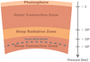 |
Fig. 1 Schematic view of Jupiter’s molecular hydrogen envelope. Low pressures (≲1 bar) correspond to the radiative photosphere, which based on chemistry codes is characterised by nitrogen-bearing clouds. Below is an outer convective zone that sits on top of a potential radiative layer. The radiative layer extends from ∼103–104 bar, at which refractory species condense. At pressures ≳104 bar, the atmosphere is convective again. We only show several condensing species for illustrative purposes. The structure of Saturn would be similar, although with a different zonal wind depth. |
2 Method
2.1 Atmospheric composition
To assess the existence of a stable radiative layer in the molecular hydrogen envelope of gas giants, we need to assume an atmospheric composition. In this section, we outline the general knowledge of the atmospheric composition of Jupiter and Saturn, and explain how the levels inaccessible to observations are modelled.
Atmospheric remote sensing from missions like Juno, Galileo, and Cassini has provided detailed insights into the atmospheric compositions of Jupiter and Saturn. These measurements generally show that both planets’ atmospheres are enriched in heavy elements1, with Jupiter exhibiting about three times solar enrichment and Saturn around eight times solar. For Jupiter, we have additional in situ measurements by the Galileo probe down to the 20 bar level, which revealed a slight depletion in helium, Yatm = 0.238 ± 0.005 (~0.8 times solar; von Zahn et al. 1998; Niemann et al. 1998). This suggests that some helium rain has occurred on Jupiter. In contrast, Saturn’s atmospheric helium abundance remains uncertain due to the lack of in situ measurements. Remote measurements by Voyager (Yatm = 0.180.25; Conrath & Gautier 2000), Cassini (Yatm = 0.15 8–0.217; Koskinen & Guerlet 2018), and Cassini Grand Finale Tour (Yatm = 0.075–0.130; Waite et al. 2018) suggest that Saturn’s atmosphere shows a greater helium depletion compared to Jupiter. This is consistent with predictions from evolution models (Nettelmann et al. 2015; Mankovich & Fortney 2020; Howard et al. 2024), which suggest a more pronounced helium rain process in Saturn due to its colder interior. Helium constitutes the second-largest mass fraction in gas giants and its abundance influences the temperature gradients in the deep atmosphere, which in turn controls the chemistry of the planet. Since pressures above ∼300 bar are inaccessible to current space missions, modelling the atmospheric composition at these depths requires one to assume a thermal profile. In this work, we model the temperature-pressure profile (TP profile) of the planet as a dry adiabat, with a 1-bar temperature fixed to the value given in Table 1. The adiabatic gradient was computed using the Chabrier et al. (2019) equation of state for dense H-He mixtures and the non-ideal mixing terms from Howard & Guillot (2023) as
 (1)
(1)
Here, SH and SHe denote the specific entropy of pure hydrogen and helium, respectively, and ∆S = Yatm(1 – Yatm)Smix is the entropy mixing term. We adopted a helium abundance of Yatm = 0.238 for Jupiter, while for Saturn we used Yatm = 0.204. For pressures below 1 bar, we used temperatures derived from in situ measurements by the Galileo probe for Jupiter (Seiff et al. 1998) and from Voyager radio-occultation data for Saturn (Lindal et al. 1985). We computed the chemistry of the planets along the resulting TP profiles using the equilibrium chemistry code FastChem (Kitzmann et al. 2024). Due to the high temperatures (∼1000–2000 K) and pressures (∼103–104 bar) relevant to this study, it is reasonable to assume that chemical timescales are shorter than dynamical ones, justifying the use of equilibrium chemistry. To model the removal of species in the gas phase into the condensate phase and their subsequent settling into cloud layers, we adopted the rainout approximation (Lodders & Fegley 2002). We show the gas and condensate chemistry of Jupiter using this approach in Fig. 2. In these calculations, the abundance of all heavy elements was set to three times the solar value of Asplund et al. (2021). As was expected, the atmosphere is dominated by H2 and He gas, with other molecules such as H2O, CH4 , and NH3 also abundant throughout in gas form. At pressures ≳1000 bar, alkali species such as K, Na, and NaH become abundant, which aligns with the onset of the stable radiative layer in Jupiter determined by Guillot et al. (1994a). Deeper in the atmosphere, metal hydrides and oxides form, and the abundance of free electrons increases. Condensation also plays a key role. Based on chemistry models, a water crystalline layer is expected around the 1-bar level of Jupiter. Around 100 bar, alkali species condense out of the atmosphere, which causes them to only become abundant in gas form at deeper levels. At even higher pressures, in the region of the potential radiative zone, refractory species such as silicates and iron condense, forming cloud layers, as is shown in the lower panel of Fig. 2. Saturn’s chemistry is quite similar to Jupiter’s, but its slightly cooler temperature causes elements like K and Na, and metal hydrides and oxides, to form at higher pressures. Similarly, condensation occurs at higher pressures, and the mixing ratios of most species are greater due to Saturn’s higher metallicity.
Fundamental properties of Jupiter and Saturn.
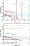 |
Fig. 2 Chemistry of Jupiter assuming an abundance of three times solar for all heavy elements. The upper panel applies to the gas chemistry, while the lower panel gives the condensate chemistry. The approximate pressure range for the potential radiative zone is shown by the shaded blue area. |
2.2 Heat transport of giant planets
In the H2 -envelope, the main mechanisms to transport internal energy are radiation and convection. In this work, we use the Schwarzschild stability criterion (Schwarzschild & Härm 1958) to determine the dominant mechanism. Deep in the atmosphere, where the optical depth is high, the diffusion approximation must hold. Under these conditions, the Rosseland-mean opacity, κR, controls the efficiency of radiative heat transport (e.g. Rybicki & Lightman 1986). It is defined as
 (2)
(2)
where κν is the monochromatic opacity and Bν is the Planck function. From the definition of the radiative temperature gradient (e.g. Guillot et al. 1994a) and the Schwarzschild stability criterion, it can be shown that if κR of a layer exceeds a critical value,
 (3)
(3)
it becomes convective. Here, P and T are the pressure and temperature of the layer, and g is the gravitational acceleration, which is assumed to be independent of depth in this study. Teff corresponds to the effective temperature of a layer and is derived from the total luminosity transported at that level. At high optical depths, all the irradiated flux has been absorbed so that Teff is given by the internal energy flux alone. Since we adopted the diffusion approximation to describe the radiative heat transport, we assume that a layer is always optically thick when computing Teff. As a result, we used Teff = 107.19 ± 0.57 K for Jupiter, and Teff = 84.13 ± 1.48 K for Saturn, which was derived from the internal energy fluxes given in Table 1. We realise that our treatment of Teff may not be valid at pressures <1 bar, where the optical depth is low and the irradiated flux needs to be accounted for, which causes Teff to increase slightly. In addition, at low optical depth the diffusion approximation breaks down, which implies that the application of κR is invalid. In this regime, the radiative transfer equation has to be solved to determine the radiative temperature gradient. However, the main focus of this study is the kilobar regime, where our treatment of Teff and Eq. (3) is valid. From Eq. (3), it becomes clear that the presence of a radiative zone in gas giant atmospheres is controlled by opacities. We shall describe our treatment of radiative opacity calculations in the following section.
2.3 Opacity calculations
In this section, we describe the calculations of opacities used in this work. In the region of a potential radiative zone (∼1000– 2000 K), the Planck function peaks around 1 µm. Consequently, we considered a spectral domain from 0.1 to 200 µm to compute opacities. Within this range, absorption due to molecules, atoms, collision-induced absorption (CIA), free electrons, and scattering all contribute to κR . In general, we calculated the absorption cross-sections over a grid of temperatures and pressures, which covers a temperature range from 100 to 5000 K with 50 linearly spaced points, and a pressure range from 10−1 to 105 bar with 26 points evenly spaced in log. The radiative opacities used in this study, along with tables of κR , are publicly available in the Zenodo repository2.
2.3.1 Atomic line absorption
This study considers the opacities of neutral atoms: Ca, Fe, Mg, Mn, Ni, Ti, V, Na, and K. We focus on atomic species that appear as condensates in the equilibrium chemistry code, ensuring their correct removal from the gas phase. While additional atomic species could be considered, their opacities are far less significant compared to molecular opacities. We calculated the absorption cross-sections of the non-alkali atoms in a uniform way using data from NIST (National Institute of Standards and Technology 2001) and the Vienna Atomic Line Data (VALD – Ryabchikova et al. 2017). We implemented our own atomic opacity calculator and shall now outline the main equations involved in these calculations.
Atomic (and molecular) absorption lines are described by an integrated line strength, S , which can be calculated assuming local thermodynamic equilibrium. For a transition from a level, i, to a higher level, j, we have (in cm g−1 )
 (4)
(4)
where, Ei and Ej are the excitation energies in cm−1 of the ith and jth level. The factors, 𝑔i and fij, correspond, respectively, to the statistical weight of the ith energy level and the oscillator strength of the transition. We retrieved the product of ɡi fij values from VALD. The partition function of the species is given by Q(T), and we computed it using the statistical weights from NIST.
Absorption lines are broadened due to thermal and pressure effects. Thermal effects produce a Gaussian line profile with a half width at half maximum (HWHM; in cm−1 ; Hill et al. 2013),
 (5)
(5)
where ν0 is the line centre in wavenumber and m is the mass of the species.
Pressure effects influence the lifetime of an energy state, which in turn specifies the broadening of the absorption line. In general, the most important pressure broadening effect in a dense medium is Van der Waals broadening. Another, less significant effect, is natural broadening as a consequence of the uncertainty principle (Gray 2008). Both effects introduce a Lorentzian absorption profile, with a combined HWHM (in cm−1 ) given by (Sharp & Burrows 2007),
![${\gamma _{\rm{L}}} = {1 \over {4\pi {\rm{c}}}}\left[ {{\gamma _{\rm{W}}}\left( {{C_{{{\rm{H}}_2}}}{N_{{{\rm{H}}_2}}} + {C_{{\rm{He}}}}{N_{{\rm{He}}}}} \right){{\left( {{T \over {{{10}^4}{\rm{K}}}}} \right)}^{3/10}} + {\gamma _N}} \right],$](/articles/aa/full_html/2025/01/aa52860-24/aa52860-24-eq6.png) (6)
(6)
where γW and γN are the Van der Waals and natural broadening coefficients, respectively, and were retrieved from VALD.  and NHe are the number densities of H2 and He, respectively. The coefficients,
  and CHe = 0.42, account for the different polarisabilities of H2 and He (Kurucz & Furenlid 1979). It is evident that in Eq. (6) we assume that atoms are only affected by perturbation from H2 and He, which are the most abundant per- turbers of gas giant atmospheres. For some transitions, Van der Waals broadening coefficients, γW , are unavailable. In this case, we define the Lorentzian HWHM (in cm−1 ) as (Schweitzer et al. 1996; Sharp & Burrows 2007),
![${\gamma _{\rm{L}}} = {{1.664461} \over {2{\rm{c}}}}{\left( {{{\rm{k}}_{\rm{B}}}T} \right)^{3/10}}\mathop \sum \limits_p \left[ {{{\left( {{1 \over m} + {1 \over {{m_p}}}} \right)}^{3/10}}C_{6,p}^{2/5}{N_p}} \right] + {{{\gamma _{\rm{N}}}} \over {4\pi {\rm{c}}}},$](/articles/aa/full_html/2025/01/aa52860-24/aa52860-24-eq9.png) (7)
(7)
where mp and Np are the mass and number density of the perturber. As in Eq. (6), we only considered the most abundant perturbers, H2 and He. The parameter C6,p is known as the interaction constant for Van der Waals interactions of a specific perturber. In general, for a transition between an energy level, Ei , to Ej, it is given as (in cm6 s−1)
![${C_{6,p}} = 1.01 \cdot {10^{ - 32}}{{{\alpha _p}} \over {{\alpha _{\rm{H}}}}}{(Z + 1)^2}\left[ {{{E_{\rm{H}}^2} \over {{{\left( {E - {E_i}} \right)}^2}}} - {{E_{\rm{H}}^2} \over {{{\left( {E - {E_j}} \right)}^2}}}} \right].$](/articles/aa/full_html/2025/01/aa52860-24/aa52860-24-eq10.png) (8)
(8)
Here, αp defines the polarisabilty of the perturber, Z is the charge of the absorber (we only consider neutral atoms, and hence we always have Z = 1), E is the ionisation potential of the absorber, αH is the polarisability of hydrogen, and EH = 13.6 eV. For the polarisabilities of H2 , and He, we used the values as given in Table 1 in Schweitzer et al. (1996). Since absorption lines have contributions from a Gaussian and Lorentzian profile, we have modelled them as Voigt profiles, which we express in terms of the real part of the normalised Faddeeva function (Gandhi et al. 2020).
Another important parameter when calculating absorption lines is the line wing cut-off, which defines the extent of the line wing on either side from the line centre. While its importance is well known in the community, there exists no first principle theory on how to treat this parameter for atoms and molecules in general. We followed the standard practice of the Exoclime team of truncating the line wings at an arbitrary distance of 100 cm−1 from the line centre (e.g. Malik et al. 2019; Whittaker et al. 2022). This is in line with the standard practice procedure for high pressures recommended by Gharib-Nezhad et al. (2023).
A different approach was used for the alkali atoms K and Na, which are very important species for the existence of a radiative layer (see Sect. 3.1). Observations of exoplanets and brown dwarfs have revealed that their resonance absorption lines exhibit strong deviations from the usual Voigt profile in their far wings (e.g. Burrows et al. 2000). This is caused by perturbations with other species, in particular H2 and He, where the potentialenergy curves describing the interactions differ from a Van der Waals broadening potential. The transitions in question are the ones of the K I resonance lines at 0.770 µm and the Na D resonance lines at 0.589 µm. There have been various studies of these line profiles in the past to determine precise interaction potentials (e.g. Tsuji et al. 1999; Burrows et al. 2000; Burrows & Volobuyev 2003; Allard et al. 2012). In this work, we use the most recent theoretical calculations of the resonance line profiles perturbed by H2 from Allard et al. (2016) for K and Allard et al. (2019) for Na. These calculations are valid up to a H2 number density of  . Hence, there will be a critical partial pressure, above which a different treatment of the resonance line profiles has to be used. For a Jupiter-like atmosphere, in which the H2 volume mixing ratio is ~88%, we can estimate that this critical pressure ranges between 10 and 600 bar for the temperatures of interest here. Unfortunately, as of this point there exist no theoretical calculations for the resonant line profiles at higher pressures. As a result, we modelled the line profiles again using a Voigt function in a similar way to the other atomic absorption lines; that is, using Eq. (6) and the Van der Waals coefficients from VALD. However, one difference from the previous calculations is that we adopted a line wing cut-off of 4500 cm−1 for the K and Na resonance lines, as is recommended by Baudino et al. (2017) to still account for their pseudo-continuum opacity spanning from the optical to the near-infrared. For all the other lines, we still employed a 100 cm−1 cut-off. We discuss the consequences of the HWHM calculation and adopted line wing cut-off for the resonance lines in Sect. 4.1.
2.3.2 Molecular and collision-induced absorption
The absorption spectrum of molecules and CIA is calculated using the opacity calculator HELIOS-K (Grimm et al. 2021). This allows one to compute absorption cross-sections from line lists and partition functions available from online databases. The opacities are computed at a resolution of 10−2 cm−1 . For molecules, we chose the ExoMol database (Tennyson et al. 2016, 2024) and used the line lists recommended by their team at the time of this work (May 2024). The only exception is CH4, for which we used the most recent HITEMP line list instead of the ExoMol recommendation, as it covers shorter wavelengths. As for the atomic lines, the molecular lines are approximated by Voigt profiles and we adopted a line wing cut-off of 100 cm−1 from the line centre. For the pressure broadening, we used the standard broadening parameters provided by the ExoMol database. The CIA corresponds to a continuum opacity rather than distinct spectral lines, so no assumption about line profiles is necessary. We used the data from HITRAN (Gordon et al. 2022) to calculate them. Tables A.1 and A.2 summarise all the molecular and CIA opacities considered in this study. In general, we calculated the absorption cross-sections over the aforementioned temperature-pressure grid. However, it is important to note that the line list of some species (CP, CrH, H2S, NaCl, NH3, TiH, and all CIA) do not extend across this entire temperature range, which explains their specific temperature ranges. To calculate opacities outside of their temperature range, we used the closest available absorption cross-sections in temperature space, without performing any extrapolation. Furthermore, we used the pre-calculated opacity data from the DACE3 database for CH4, CO2, PH3, and SiH4. These are larger molecules with billions of transitions, making the calculation of their absorption crosssections computationally very expensive. Although DACE uses a different temperature-pressure grid than the one adopted in this work, it covers the relevant conditions in which these molecules significantly contribute to κR. For H2O and NH3, which are also larger molecules, we used their available super-line lists to calculate their absorption cross-sections.
2.3.3 Bound-free and free-free absorption
At high temperatures (≳2500 K), bound-free and free-free interactions become relevant sources of opacities. In bound-free processes, a sufficiently energetic photon detaches an electron from an ion, and in free-free processes, a free electron approaches an atom or molecule, altering its potential. Both interactions result in continuous absorption of photons. In our calculations, we included bound-free absorption from H−, and free-free absorption from  , H−, and He−. We summarise the reactions, the wavelength coverage of the opacities, and the relevant references in Table A.3.
2.3.4 Rayleigh scattering
Rayleigh scattering acts as a continuous source of opacity. We included Rayleigh scattering cross-sections of the following species: CO2 (Sneep & Ubachs 2005; Thalman et al. 2014), CO (Sneep & Ubachs 2005), H2 (Allen & Cox 2000), H (Lee & Kim 2004), He (Sneep & Ubachs 2005; Thalman et al. 2014), N2 (Sneep & Ubachs 2005; Thalman et al. 2014), O2 (Sneep & Ubachs 2005; Thalman et al. 2014), and electrons (Astropy Collaboration 2022).
2.3.5 Abundance weighted-total opacities
After computing the cross-sections, we interpolated them for each species to the same wavelength grid of resolution Δλ/λ = 10000. We found that this resolution results in converging values of κR. To convert the absorption and scattering cross-sections (in cm2) into opacities (cm2 g−1 ), we multiplied them by the mixing ratio of the species and divided this by the mean molecular weight of the atmospheric layer4. As is mentioned in Sect. 2.1, we computed ĸR along a dry adiabatic TP profile of Jupiter and Saturn. The temperatures and pressures along these profiles do not exactly match our cross-section grid. Hence, we used bilinear interpolation to match the cross-sections to the temperaturepressure conditions along the profiles. The interpolation was performed in logarithmic space for pressure and linear space in temperature.
3 Results
3.1 Opacity spectra
We now want to identify the dominant sources of opacity at different depths in the atmosphere of gas giants in the Solar System. Assuming a general solar composition for the heavy elements, we focus on various layers along Jupiter’s adiabat. The following conclusions can also be applied to Saturn.
Figure 3 shows the total opacity (solid black curves) of our atmospheric Jupiter model at three different depths. The upper panel applies to a pressure of 50 bar, which corresponds to the outer convective region of Jupiter. At these conditions, the most abundant molecules in the gas phase are H2O, CH4, and NH3, all of which have strong absorption features in the infrared. Wavelengths above 1 µm contribute the most to ĸR in this layer, as is highlighted by the Planck curve (dashed grey), which acts as a weighting function to ĸR. Hence, H2O, CH4, and NH3 control the opacity and heat transport in this layer, which is a picture that persists until about 103 bar. At deeper layers, the higher density makes CIA significantly more important. The middle panel in Fig. 3 shows the opacity at a layer of 2⋅103 bar. This reflects the importance of CIA by H2 at these conditions, which now overwhelms the opacity of molecules at longer wavelengths. Below 1 µm, the absorption of alkali-bearing species, K, Na, and NaH emerges and completely dominates the shortwavelength opacity. We remind the reader that the resonance lines K I and Na D are modelled as Voigt profiles here, due to the absence of a detailed theory for their potential-energy curves describing the interaction with H2 at high pressures. The higher temperature of the layer causes the Planck function to shift to lower wavelengths, which causes the alkali species to make an important contribution to ĸR. In the absence of alkali species, ĸR of this layer would drop significantly, as no other short-wavelength absorbing species are present in considerable amounts at this depth. Moreover, because ĸR is a harmonic mean, the few absorbers in the visible spectrum can impact it much more than the numerous absorbers in the infrared. Other shortwavelength absorbing species only become abundant at layers around 104 bar. This includes metal hydrides (ex. CaH, CrH, FeH, MgH), metal oxides (e.g. CaO, MgO, TiO, VO), bound- free and free-free absorptions due to electrons, and other neutral atomic species (e.g. Ca, Fe, Mg). The lower panel in Fig. 3 gives the opacity spectrum at 2⋅104 bar, and shows the absorption of several species at short wavelengths. Hence, at high pressures a range of species contribute to ĸR, not only alkali gases.
The fact that between ~103–104 bar, alkali are the only species capable of absorbing in the visible causes them to control the existence of the radiative layer that was predicted by Guillot et al. (1994a), who did not include those opacities in their calculations. Its importance was later realised in Guillot et al. (2004), in which they found that they could prevent the radiative zone. In the next section, we shall estimate the abundance of K and Na needed to achieve this.
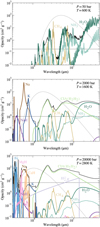 |
Fig. 3 Opacities of Jupiter at different depths, assuming a solar composition in heavy elements. The total opacity of the layer is given in black, and the opacities of individual species are given as coloured curves. The Rosseland-mean opacity, ĸR, of the layer is shown as the dashed black line and the Planck function at the relevant temperature is given as the dashed grey curve. |
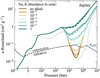 |
Fig. 4 Rosseland-mean opacity, ĸR (solid and dashed coloured curves), as a function of pressure for atmospheres with varying and Na and K abundances calculated along a Jupiter profile. The abundance of all other heavy elements is three times solar. The solid curves were computed using the Na D and K I HWHM formulation from Eq. (6), while the dashed curves use the Na D and K I HWHM formulation from Allard et al. (2016), Allard et al. (2019), Allard et al. (2023) and Allard et al. (2024). The dashed black curve corresponds to the critical opacity, ĸcrit. The dotted grey curve corresponds to ĸR from Guillot et al. (1994a). |
3.2 Conditions for a radiative zone on Jupiter
3.2.1 Deep radiative zone
Using our opacity tables, we shall now determine the atmospheric compositions needed to develop a radiative zone on Jupiter. As was seen in the previous section, K and Na are the most important elements to determine the existence of a radiative zone. Hence, we show ĸR for Jupiter for varying elemental abundances of K and Na in Fig. 4. The abundances of all the other heavy elements are fixed at three times solar. The dashed black curve corresponds to the critical opacity, ĸcrit, of Jupiter, and is evaluated using Eq. (3). For comparison, we show ĸR from Guillot et al. (1994a). As was expected, the presence of K, Na, and NaH has a significant impact on ĸR between ~ 103–104 bar. If their opacities are neglected, a radiative zone develops between ~ 103–7⋅103 bar (i.e. ~1400–2100 K). This region is comparable to the one identified by Guillot et al. (1994a). However, the radiative zone in our study is shallower due to the inclusion of opacities from metal hydrides and oxides, which were not accounted for in Guillot et al. (1994a). When the opacities of K, Na, and NaH are included, ĸR at the kilobar level increases by almost three orders of magnitude for solar abundances of K and Na. As the alkali abundance increases, the extent of the stable layer progressively shrinks at both ends until it disappears entirely and restores convection. Our opacities suggest that a significant alkali depletion of less than ~10−3 times solar is required for a radiative zone to exist in Jupiter’s molecular hydrogen envelope.
Furthermore, we find that the radiative-convection boundary of Jupiter is located around 0.5 bar. However, this result is sensitive to the H2-H2 CIA opacity, which below 200 K only covers wavelengths down to 4.167 µm (see Table A.3). Hence, it is possible that the RCB may occur at even lower pressures.
In Fig. 5, we show the effect of all the other elements, except for K, Na, H, and He, on Jupiter’s ĸR. In this case, the atmospheres are highly depleted in K and Na (10−5 times solar), while the abundances of other heavy elements are varied simultaneously. We find that, even with a high abundance of heavy elements, a radiative zone can still form deep in the atmosphere, provided there is sufficient alkali depletion. This highlights again the crucial role of K, Na, and NaH in determining whether a radiative layer develops, as no other known gas species can prevent its formation. The main effect of non-alkali heavy elements on the deep radiative zone is to determine its extent. For a heavy element abundance of 0.1 times solar (consistent with interior models), the radiative layer extends from ~5⋅102–104 bar (i.e. ~ 1200–2500 K), as opposed to ~ 103–7⋅103 bar (i.e. ~1400– 2100 K) for a three times solar abundance suggested by Juno and Galileo observations.
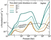 |
Fig. 5 ĸR (solid coloured curves) as a function of pressure for atmospheres with varying heavy element abundances, but fixed Na and K abundances of 10−5 times solar. The opacities were calculated along a Jupiter profile. The dashed black curve corresponds to the critical opacity, ĸcrit. |
3.2.2 Shallow radiative zone
In Fig. 5, we find that for low heavy element abundances, a second shallow radiative zone emerges between ~3–100 bar (i.e. ~200–600 K). This is related to a depletion in H2O, NH3, and CH4 , which are the main absorbers at low pressure and temperature. This radiative window was also identified by Guillot et al. (1994a) when removing the H2O opacity. From Juno and Galileo measurements, we know that a depletion in NH3 and CH4 is unlikely at low pressures. The abundance in H2O is more uncertain due to the subsolar abundance reported by the Galileo probe (Wong et al. 2004) and supersolar measurements from Juno (Li et al. 2024). The work of Wong et al. (2004) reports an O abundance of 0.289 ± 0.096 times solar abundance; however, we find that an abundance between 0.8 and 1.1 times solar is needed to align with the H2O mixing ratio measurements from the Galileo probe. This discrepancy arises because the earlier study neglected the effect of rocks and the sequestration of O atoms by these. At pressures around 10 kbar, MgO and SiO condense, and for a 0.289 solar O abundance, these species are abundant enough to almost completely remove O atoms from the atmosphere at lower pressures. As a result, the O abundance in Wong et al. (2004) is incompatible with the Galileo H2O measurement.
We re-calculated the opacities at low pressures using the measured N and C abundances of 2.61 and 3.56 times solar, respectively (Wong et al. 2004; Li et al. 2020; Guillot et al. 2022), while varying the O abundance. The abundance of K and Na has no effect in this region. The resulting ĸR are shown in Fig. 6. We find that with an O depletion of 0.1 times solar, the system is on the verge of preventing a radiative window, while for an abundance matching the Galileo measurement convection is restored. In fact, the temperature gradients of this region have been probed by the Galileo and Juno mission. During the in situ measurements, the Galileo probe found sub-adiabatic gradients between 0.5 and 20 bar, which is thought to be a manifestation of mean molecular weight gradients due to the vertical variation in the water vapour abundance (Magalhães et al. 2002). These sub- adiabatic gradients are surprising, as our opacity models predict adiabatic gradients for an O-abundance matching the one measured by the Galileo probe. While we calculated mean molecular weight gradients for a case matching the O-abundance measured by the Galileo probe, we found them to be negligible and unable to produce sub-adiabatic gradients. One possible reason for this discrepancy is the use of equilibrium chemistry to describe the shallow layers, where temperatures are relatively low (≲300 K).
Disequilibrium effects are expected in this region, which complicates the analysis. Furthermore, at pressures below ~5 bar, water condensation is expected, releasing latent heat that can influence the local temperature.
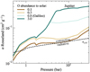 |
Fig. 6 ĸR (solid coloured curves) at low pressures for Jupiter with varying O abundances. The abundance of C is fixed to 3.56 times solar, and that of N is fixed to 2.61 times solar. The dashed black curve corresponds to the critical opacity, ĸcrit. |
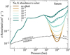 |
Fig. 7 ĸR (solid and dashed coloured curves) as a function of pressure for atmospheres with varying and Na and K abundances calculated along a Saturn profile. The abundance of all other heavy elements is eight times solar. The solid curves were computed using the Na D and K I HWHM formulation from Eq. (6), while the dashed curves use the Na D and K I HWHM formulation from Allard et al. (2016), Allard et al. (2019), Allard et al. (2023) and Allard et al. (2024). The dashed black curve corresponds to the critical opacity, ĸcrit. |
3.3 Conditions for a radiative zone on Saturn
Having assessed the conditions for a radiative zone on Jupiter, we can now apply the same analysis to Saturn. Figure 7 shows ĸR for Saturn with varying Na and K abundances, while the abundance of other heavy elements is fixed at eight times solar. Similar to Jupiter, a radiative zone forms only with sufficient alkali depletion. Non-alkali metals are unable to prevent the formation of the radiative layer and will only control its extent. Due to Saturn’s lower mass, the critical opacity, ĸcrit, is lower than Jupiter’s, implying that less Na and K are required to inhibit the development of a radiative zone. We find that an alkali abundance below ~10−4 is required for a radiative layer to form, and it develops at higher pressures than on Jupiter, between ~4⋅103 and 2⋅104 bar.
The radiative-convection boundary on Saturn is located at ≲0.4 bar. The exact location cannot be determined because FastChem does not converge at temperatures below 100 K. As a result, we can only compute ĸR down to 0.4 bar for Saturn.
3.4 Thermal profiles
One of the main effects of a radiative zone in the deep atmosphere of a planet is to introduce deviations from an adiabatic TP profile. In Fig. 8, we show TP profiles of Jupiter and Saturn in the presence of a radiative zone (shown as shaded regions). This was achieved by sufficiently depleting the atmosphere in K and Na, while keeping the abundance of the other heavy elements fixed at three and eight times solar for Jupiter and Saturn, respectively. As was anticipated, a radiative zone results in a cooler interior of the planet, given its subadiabatic nature (∇rad < ∇ad). For Jupiter, a significant depletion in alkali results in a temperature at the bottom of the radiative zone that is at most ~25% smaller than the one of the dry adiabatic model. The temperature difference is slightly less than the 30% found in Guillot et al. (1994b). The origin of this is most likely the inclusion of more opacity sources in this work, which increases the temperature gradients in the radiative zone. We expect that the temperature difference propagates to the centre of the planet, as the convective gradients of the dry adiabat and the radiative zone model are similar at deeper levels. As the alkali abundance increases, the temperature difference decreases as a result of the larger temperature gradient in the radiative zone.
For Saturn, a significant depletion in alkali leads to a smaller temperature difference at the bottom of the radiative zone relative to a dry adiabat model. This is related to the fact that the radiative zone is located at deeper levels in Saturn, which reduces its effect. In addition, the heavy element abundance is larger on Saturn, which increases the temperature gradient in the radiative zone. We find that the radiative zone can lead to an interior which is at most ~10% colder than the adiabatic model, which again is slightly less than the 15% temperature decrease reported by Guillot et al. (1994b).
Lowering the planet’s interior temperature has significant implications, including shifting the locations of key phase transitions, such as H/He separation (Salpeter 1973; Stevenson 1979) and the transition to metallic hydrogen (Sano et al. 2011; Loubeyre et al. 2012). For a cooler interior, these transitions occur deeper within the planet. Another consequence of a cooler interior is to increase the core density. Since the mean density of the planet is constrained by observations, an increase in the central density must be balanced by a decrease in density in the gaseous envelope. In other words, the atmospheric heavy element abundance, Zatm, is lower for interior models that include a radiative zone compared to adiabatic models.
The presence of a radiative zone also modifies the internal entropy of the planet. By definition, for a fully convective interior, without any phase transitions, the specific entropy, S, is constant throughout the planet. However, in a radiative zone, S will change due to its non-adiabatic behaviour. We find that S decreases from the top to the bottom of the radiative zone by a magnitude of up to ∆S ≈ −4⋅107 erg K−1g−1 for Jupiter and ∆S ≈ −2⋅107 erg K−1 g−1 for Saturn. The magnitude, ∆S, decreases as the abundance of K and Na increases until the medium becomes fully convective again.
4 Discussion
4.1 Half width at half maximum and cut-off of K I and Na D lines
In this paper, we have used the calculations from Allard et al. (2016) and Allard et al. (2019) to model the K I and Na D resonance lines (see Sect. 2.3.1). At high pressure, we switched to Voigt profiles due to the lack of applicable theories and experiments. In Jupiter and Saturn, K and Na only become abundant at pressures ≳1000 bar, at which point we modelled their resonance lines as Voigt profiles with a Lorentzian HWHM based on Van der Waals broadening parameters and a cut-off value of 4500 cm−1 for the line wings. Alternative formulations for the Lorentzian HWHM of the resonance lines exist, which depend on the assumed potential energy curve of the two colliding partners. To assess the impact on our results, we explored HWHM formulations from various sources: Allard et al. (2016) for the K- H2 potential, Allard et al. (2024) for the K-He potential, Allard et al. (2019) for the Na-H2 potential, and Allard et al. (2023) for the Na-He potential. We find that the K and Na resonance feature is narrower when using the Allard HWHM treatment. However, the differences in κR are negligible, and our conclusions remain unchanged regardless of the Lorentzian HWHM formulation used (see Figs. 4 and 7 dashed coloured curves).
The choice of line wing cut-off value is significantly more important. Baudino et al. (2017) and Chubb et al. (2021) recommend a cut-off value of 4500 cm−1, although this is not based on any specific theoretical justification, but rather on the observation that the K I and Na D line wings extend significantly from their core, κR of Jupiter assuming different line wing cut-offs are shown in Fig. 9. We find that increasing the cut-off value from 4500 cm−1 to 10000 cm−1 (dotted curve) has no notable effect on κR, and, as before, an alkali depletion of less than 10−3 times solar is required to develop a radiative zone. In contrast, reducing the cut-off value to 1000 cm−1 (dashed curve) substantially decreases κR. In this scenario, a radiative layer can develop even with alkali abundances close to solar levels. While it is unlikely that the Na D and K I line wings only extend to 1000 cm−1, given their behaviour at lower pressures, this example highlights the importance of improving our understanding of their profiles at high pressures. We emphasise that regardless of the cut-off value, a Na abundance above solar should still be sufficient to prevent a radiative zone due to the opacity of NaH.
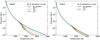 |
Fig. 8 Temperature pressure profiles of Jupiter (left panel) and Saturn (right panel) for different K and Na abundances. The parts where radiative zones exist are indicated as the shaded regions. The adiabatic models are given as green curves. |
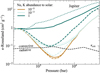 |
Fig. 9 κR of Jupiter for varying Na and K abundances and adopting different line wing cut-off values for the KI and Na D features. The solid lines represent the baseline cut-off value of 4500 cm−1, the dotted lines use a cut-off value of 10000 cm−1, and the dashed lines use a cut-off value of 1000 cm−1. The dashed black curve corresponds to the critical Opacity, κcrit. |
4.2 Constraints on alkali abundance
While we have determined how much K and Na is needed to develop a deep radiative layer on Jupiter and Saturn, the true abundance of these elements is unclear. Since they are expected to condense out of the atmosphere around 800 K, they should not be directly observable in cooler planets like Jupiter and Saturn. The resonance feature Na D has been observed in ‘transmission’ spectra of Jupiter (Montañés-Rodríguez et al. 2015), although this feature is likely related to the continuous volcanic outgassing from the galilean moon Io (Lellouch et al. 2003; Mendillo et al. 2004) or cometary impacts (Noll et al. 1995). Hence, these observations should not be representative of the alkali abundance at deeper levels.
Recent brightness temperature and limb darkening observations by the MWR instrument on Juno attempted to constrain the abundance of K and Na, as a proxy for the free electron abundance at the kilobar level. The initial results indicate a high depletion in alkali in the range of 10−5 to 10−2 times solar (Bhattacharya et al. 2023). This level of depletion would potentially allow for the existence of a stable radiative layer in Jupiter, based on the calculations performed in this study. However, this study neglected the importance of anions, which act as a sink of free electrons, and a reassessment of the analysis suggested a higher abundance for both K and Na of order 10−1 times solar (Aglyamov et al. 2025). Although there still seems to be a subsolar abundance in K and Na on Jupiter, our results and these measurements suggest that developing a radiative zone on the planet at this time would be challenging. The origin of such a depletion is unclear and could be explained through an unconventional planet formation mechanism, where Jupiter accreted a subsolar abundance of alkali metals. Alternatively, it could imply that the planet’s interior is not well mixed, such that most alkalis are locked in the core. A diluted core, as has been proposed by recent interior models (Wahl et al. 2017; Nettelmann et al. 2021; Miguel et al. 2022), can reduce the efficiency of con-vective mixing, and it has been shown that for Jovian conditions it has an erosion lifetime exceeding Jupiter’s age (Fuentes et al. 2024). We emphasise that the alkali measurements provided by the MWR observations are interpreted as global abundances on Jupiter and are expected to vary spatially due to the complexity of the planet’s atmosphere. Alternative measurements of Jupiter’s atmospheric alkali levels would be invaluable in confidently ruling out the existence of a radiative layer.
Alkali metals have been detected in hot gas giant exoplanets. An indirect measurement includes Kepler-7b, where an alkali depletion of 10−1–10−2 was inferred based on the planets high albedo (Demory et al. 2011). Another subsolar abundance in alkali was observed in the transit spectra of HAT-P-lb, with ![$[{\rm{Na}}/{\rm{H}}] = - 0.77_{ - 0.44}^{ + 0.50}$](/articles/aa/full_html/2025/01/aa52860-24/aa52860-24-eq13.png) and [K/H] < −1.25 (Chen et al. 2022). While these measurements suggest alkali depletion on gas giants, solar to super-solar measurements also exist. Examples include WASP-76b with
and [K/H] < −1.25 (Chen et al. 2022). While these measurements suggest alkali depletion on gas giants, solar to super-solar measurements also exist. Examples include WASP-76b with ![$[{\rm{Na}}/{\rm{H}}] = 0.649_{ - 0.902}^{ + 0.511}$](/articles/aa/full_html/2025/01/aa52860-24/aa52860-24-eq14.png) (Fu et al. 2021) or WASP-96b with
(Fu et al. 2021) or WASP-96b with ![$[{\rm{Na}}/{\rm{H}}] = 1.32_{ - 0.48}^{ + 0.36}$](/articles/aa/full_html/2025/01/aa52860-24/aa52860-24-eq15.png) (Nikolov et al. 2018, 2022). Given the discrepancy in alkali abundances and the small sample size of their detection in gas giant exoplanets, we should refrain from drawing any conclusions about the alkali abundance on Jupiter or Saturn based on exoplanet observations. However, we note that repeating these calculations to giant exoplanets with known alkali abundances would be of great interest.
(Nikolov et al. 2018, 2022). Given the discrepancy in alkali abundances and the small sample size of their detection in gas giant exoplanets, we should refrain from drawing any conclusions about the alkali abundance on Jupiter or Saturn based on exoplanet observations. However, we note that repeating these calculations to giant exoplanets with known alkali abundances would be of great interest.
4.3 Impact of cloud opacities
As is pointed out in Sect. 2.1, heavy elements condense at high temperatures and can form cloud decks. Molecules that condense between 103 and 104 bar for Jupiter and Saturn conditions are, for example, Fe, MgO, Mg2SiO4, MnS, and SiO. This represents an additional source of opacity that also extends to wavelengths < 1 µm. We shall estimate here the impact of these five condensates on κR.
Modelling cloud formation and their opacity involves a description of condensation, coagulation and coalescence, sedimentation, and eddy mixing. Since at high temperatures (>1000 K), eddy mixing timescales are expected to be much slower than the ones of other processes, the structure of clouds will be similar to that determined by the condensates vapour pressure (i.e. the output of FastChem). We simplified the coagulation and sedimentation process using the Ackerman & Marley (2001) model, which allows one to parametrise the mean radius and number density of cloud particles in a layer using two parameters, frain (ratio of mass-weighted sedimentation velocity to convective velocity scale), and σg (geometric standard deviation in lognormal size distributions of condensates). We defined frain = 3 and σg = 2, which results in mean radii ranging from ~1–3 µm. We computed the absorption and scattering cross-sections of condensates using the code LX-MIE (Kitzmann & Heng 2017) and the compilation of the optical constants therein. Figure 10 shows κR of Jupiter, including the contributions from condensates and assuming a heavy element abundance of three times solar. The dotted coloured bars represent the extent of the cloud deck for each condensate. At low K and Na abundances, sharp peaks in κr appear, corresponding to the base of cloud decks where condensates have settled, creating regions of higher opacity. The first peak, around 2 ⋅ 103 bar, is due to MnS condensates, while the second and third peaks are caused by SiO and MgO condensates, respectively. As the abundance of K and Na increases, these cloud-related features disappear, as alkali opacities dominate. We find that the MnS cloud is able to elevate κR above the critical value, κcrit, shrinking the extent of the radiative layer. The cloud base of the other condensates resides at higher pressure, ≳104 bar, and as a result they are unable to prevent the radiative zone. Varying the heavy element abundance alters the location of these cloud bases; generally, a higher abundance raises the vapour saturation pressure, pushing the cloud deck to higher pressures. Conversely, decreasing the abundance shifts the cloud base into the radiative zone but also reduces its opacity. Hence, the condensates considered here are incapable of fully preventing the radiative zone. In this analysis, we restricted ourselves to condensates for which optical properties were available. We found that condensates of Cu, Cr2O3, CaTiO3, CaSiO3, and CaMgSi2O6 form cloud bases in the region of the radiative zone, although their mixing ratios are smaller than that of MnS at three times solar metallicity. However, calculating κR with the contribution of their opacities would be of great interest.
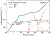 |
Fig. 10 Solid curves give κR of Jupiter for varying Na and K abundances and including the opacities from the condensates Fe, MgO, Mg2 SiO4, MnS, and SiO. The abundance of all other heavy elements was set to three times solar. The regions where each condensate contributes to κr are illustrated by the bars. The dotted curves give κR without the contribution from condensate opacities. The dashed black curve corresponds to the critical opacity, κcrit. |
4.4 Validity of Schwarzschild criterion
As is outlined in Sect. 2.2, we employed the Schwarzschild stability criterion to determine the dominant heat transport mechanism. However, this criterion applies to homogeneous and dry conditions, and the presence of condensation can violate these assumptions. When a species condenses, this produces a vertical gradient in the mixing ratio of that species in the gas phase, with the mixing ratio increasing with depth. As a result, when condensation takes place, the mean molecular weight of the atmosphere, denoted as µ, can increase at greater depths (i.e.  ), thereby stabilising the medium against convection. This is known as the Ledoux stability criterion (Ledoux 1947),
 (9)
(9)
Hence, it is possible for a radiative layer to exist for a supera-diabatic gradient. The next consequence of condensation is that, within a convective layer, the temperature profile follows the ‘moist’ adiabat,  , instead of the dry adiabat, ∇ad. This change occurs due to the release of latent heat during condensation, which contributes to a positive buoyancy and facilitates convection; that is,
  .
.
Since condensation of refractory materials occurs in the region where a radiative layer may exist in Jupiter and Saturn, it is reasonable to question the use of the Schwarzschild criterion in this study. We calculated mean molecular weight gradients for atmospheres assuming different abundances of metals, and found that they never exceeded a value of 0.2∇ad at high pressures. While this introduces a change in the critical opacity, κR, its effect is negligible and will not change the results of this work. At lower pressures, in the region where H2O condenses, the effect of mean molecular weight gradients is more pronounced and is known to stabilise Jupiter’s atmosphere in the 5 µm hotspot (Magalhães et al. 2002).
We have also estimated the moist adiabat caused by the condensation of MgO at high pressures. We chose MgO due to its large known latent heat of vapourisation L = 8.27 kJ g−1 (Mahmoud & Yabe 2017) compared to other condensing species with known values (e.g. L = 6.34 kJ g−1 for Fe, see Zhang 2011). Following Eq. (11) in Leconte et al. (2017), we find that the fractional difference between the dry and moist adiabat is of order 10−8, which justifies the use of the dry adiabat in this work.
5 Conclusions
We have calculated κR for the molecular hydrogen envelopes of Jupiter and Saturn. Our opacity tables are the most comprehensive to date, covering pressures up to 105 bar and incorporating the most abundant molecules found in gas giants, along with contributions from free electrons, various metal hydrides and oxides, and atomic species. We investigated different atmospheric composition and determined the conditions needed to develop a radiative zone at the kilobar level in Jupiter and Saturn today.
We found that K, Na, and NaH are the only species capable of restoring convection in the kilobar regime. The main effect of other opacity species is to control the width of a radiative zone. For significant depletions in the elemental abundances of K and Na, a radiative zone develops on Jupiter between ~ 103 – 7 ⋅ 103 bar, while on Saturn it exists deeper in the envelope between ~4 ⋅ 103 – 2 ⋅ 104. For K and Na abundances exceeding ~10−3 times solar on Jupiter and ~10−4 times solar on Saturn, convection is restored. The radiative zone identified in this study is too shallow to control the depth of Jupiter’s zonal winds as is suggested by Christensen & Wulff (2024) and Moore et al. (2022). At pressures ≳104 bar, the radiative opacities are more than two orders of magnitude too large too allow for stable radiative layers at greater depths. However, this does not rule out the possibility of stable layers at deeper levels, as conductive opacities were not calculated in this study. In a highly conductive fluid, heat transport can occur through conduction, potentially resulting in stable conductive layers.
We determined new thermal profiles for Jupiter and Saturn, assuming sufficient depletions of K and Na to form a radiative layer. Our results show that the presence of a radiative zone lowers Jupiter’s interior temperature by up to 25% compared to an adiabatic model, while Saturn’s interior temperature decreases by up to 10%. The cooler interior has significant implications for the inferred metallicity of the planet’s gaseous envelope in interior models. Additionally, a radiative zone decreases the specific entropy by up to ΔS ~ −4 ≳ 107erg K−1 g−1 for Jupiter and AS ≈ −2 ⋅ 107erg K−1 g−1 for Saturn.
We emphasise that these results are strongly influenced by the cut-off value for the line wings of the K I and Na D resonance lines, as is discussed in Sect. 4.1. Developing a theory for these lines in the kilobar regime would enhance the accuracy of this study. Furthermore, it is important to mention that molecules without available line lists could influence our results. For instance, potassium hydride (KH), which forms at conditions similar to NaH, likely has absorption features below 1 µm, and its absence in our opacity tables could affect the results.
In summary, we show that a substantial depletion in K and Na is needed to develop a radiative zone in the deep atmosphere of Jupiter and Saturn. Current estimates of their abundances on Jupiter suggest subsolar levels, which would restore convection at the present day.
We emphasise that, to either confidently rule out the possibility of a radiative zone or determine if it can resolve the conflict between interior models and observations, several critical steps are required. First, new methods of probing alkali should be developed to gather additional measurements and confirm the current constraints on their abundance. Second, we need to advance the theory describing the K I and Na D line profiles when perturbed by H2 and He, particularly at higher pressures. Finally, understanding the dynamics and evolution of the radiative zone is essential. This includes exploring molecular diffusion across the layer and investigating its properties and existence during earlier stages of planetary evolution.
Data availability
The radiative opacities used in this study, along with κr tables for Jupiter and Saturn, are available at https://doi.org/10.5281/zenodo.14507606.
Acknowledgements
We thank the referee for valuable comments which helped improve the manuscript. This project has received funding from the European Research Council (ERC) under the European Union’s Horizon 2020 research and innovation programme (grant agreement no. 101088557, N-GINE). This publication is part of the project ENW.GO.001.001 of the research programme “Use of space infrastructure for Earth observation and planetary research (GO), 2022-1” which is (partly) financed by the Dutch Research Council (NWO). TG benefited from support from CNES as part of the Juno mission.
Appendix A Tables
Molecular opacities used in this work. * super-line lists were used for H2O and NH3.
[1]: Ram et al. (2014); Bernath (2020); Qin et al. (2021) [2]: Burrows et al. (2002); Chubb et al. (2018); Bernath (2020) [3]: Li et al. (2015); Coxon & Hajigeorgiou (2015); Somogyi et al. (2021) [4]: Shemansky (1969); Western (2017); Western et al. (2018); Jans (2024)
Collision-induced absorption used in this work.
Bound-free and free-free absorptions considered in this work.
References
- Abel, M., Frommhold, L., Li, X., & Hunt, K. 2011, J. Phys. Chem., 115, 6805 [CrossRef] [Google Scholar]
- Abel, M., Frommhold, L., Li, X., & Hunt, K. L. C. 2012, J. Chem. Phys., 136, 044319 [NASA ADS] [CrossRef] [Google Scholar]
- Ackerman, A. S., & Marley, M. S. 2001, ApJ, 556, 872 [Google Scholar]
- Aglyamov, Y. S., Atreya, S. K., Bhattacharya, A., et al. 2025, Icarus, 425, 116334 [NASA ADS] [CrossRef] [Google Scholar]
- Al Derzi, A. R., Furtenbacher, T., Tennyson, J., Yurchenko, S. N., & Császár, A. G. 2015, J. Quant. Spec. Radiat. Transf., 161, 117 [NASA ADS] [CrossRef] [Google Scholar]
- Allard, N. F., Kielkopf, J. F., Spiegelman, F., Tinetti, G., & Beaulieu, J. P. 2012, A&A, 543, A159 [NASA ADS] [CrossRef] [EDP Sciences] [Google Scholar]
- Allard, N. F., Spiegelman, F., & Kielkopf, J. F. 2016, A&A, 589, A21 [NASA ADS] [CrossRef] [EDP Sciences] [Google Scholar]
- Allard, N. F., Spiegelman, F., Leininger, T., & Molliere, P. 2019, A&A, 628, A120 [NASA ADS] [CrossRef] [EDP Sciences] [Google Scholar]
- Allard, N. F., Myneni, K., Blakely, J. N., & Guillon, G. 2023, A&A, 674, A171 [NASA ADS] [CrossRef] [EDP Sciences] [Google Scholar]
- Allard, N. F., Kielkopf, J. F., Myneni, K., & Blakely, J. N. 2024, A&A, 683, A188 [NASA ADS] [CrossRef] [EDP Sciences] [Google Scholar]
- Allen, C. W., & Cox, A. N. 2000, Allen’s Astrophysical Quantities (Springer Science & Business Media) [Google Scholar]
- Asplund, M., Amarsi, A. M., & Grevesse, N. 2021, A&A, 653, A141 [NASA ADS] [CrossRef] [EDP Sciences] [Google Scholar]
- Astropy Collaboration (Price-Whelan, A. M., et al.) 2022, ApJ, 935, 167 [NASA ADS] [CrossRef] [Google Scholar]
- Azzam, A. A. A., Tennyson, J., Yurchenko, S. N., & Naumenko, O. V. 2016, MNRAS, 460, 4063 [NASA ADS] [CrossRef] [Google Scholar]
- Barton, E. J., Chiu, C., Golpayegani, S., et al. 2014, MNRAS, 442, 1821 [NASA ADS] [CrossRef] [Google Scholar]
- Baudino, J.-L., Mollière, P., Venot, O., et al. 2017, ApJ, 850, 150 [Google Scholar]
- Bell, K. L. 1980, J. Phys. B, 13, 1859 [CrossRef] [Google Scholar]
- Bernath, P. F. 2020, J. Quant. Spec. Radiat. Transf., 240, 106687 [NASA ADS] [CrossRef] [Google Scholar]
- Bhattacharya, A., Li, C., Atreya, S. K., et al. 2023, ApJ, 952, L27 [NASA ADS] [CrossRef] [Google Scholar]
- Bjoraker, G. L., Wong, M. H., de Pater, I., et al. 2018, AJ, 156, 101 [NASA ADS] [CrossRef] [Google Scholar]
- Bolton, S. J., Lunine, J., Stevenson, D., et al. 2017, Space Sci. Rev., 213, 5 [CrossRef] [Google Scholar]
- Borysow, A., & Frommhold, L. 1986, ApJ, 304, 849 [NASA ADS] [CrossRef] [Google Scholar]
- Brady, R. P., Yurchenko, S. N., Tennyson, J., & Kim, G.-S. 2023, MNRAS, 527, 6675 [NASA ADS] [CrossRef] [Google Scholar]
- Burrows, A., & Volobuyev, M. 2003, ApJ, 583, 985 [Google Scholar]
- Burrows, A., Marley, M. S., & Sharp, C. M. 2000, ApJ, 531, 438 [NASA ADS] [CrossRef] [Google Scholar]
- Burrows, A., Ram, R. S., Bernath, P., Sharp, C. M., & Milsom, J. A. 2002, ApJ, 577, 986 [NASA ADS] [CrossRef] [Google Scholar]
- Burrows, A., Dulick, M., C.W. Bauschlicher, J., et al. 2005, ApJ, 624, 988 [NASA ADS] [CrossRef] [Google Scholar]
- Bézard, B., Lellouch, E., Strobel, D., Maillard, J.-P., & Drossart, P. 2002, Icarus, 159, 95 [CrossRef] [Google Scholar]
- Campbell, J. K., & Synnott, S. P. 1985, AJ, 90, 364 [NASA ADS] [CrossRef] [Google Scholar]
- Cavalié, T., Lunine, J., & Mousis, O. 2023, Nat. Astron., 7, 678 [CrossRef] [Google Scholar]
- Chabrier, G., Mazevet, S., & Soubiran, F. 2019, ApJ, 872, 51 [NASA ADS] [CrossRef] [Google Scholar]
- Chen, G., Wang, H., van Boekel, R., & Pallé, E. 2022, AJ, 164, 173 [NASA ADS] [CrossRef] [Google Scholar]
- Christensen, U. R., & Wulff, P. N. 2024, PNAS, 121, e2402859121 [NASA ADS] [CrossRef] [Google Scholar]
- Chubb, K. L., Naumenko, O., Keely, S., et al. 2018, J. Quant. Spec. Radiat. Transf., 218, 178 [NASA ADS] [CrossRef] [Google Scholar]
- Chubb, K. L., Rocchetto, M., Yurchenko, S. N., et al. 2021, A&A, 646, A21 [NASA ADS] [CrossRef] [EDP Sciences] [Google Scholar]
- Coles, P. A., Yurchenko, S. N., & Tennyson, J. 2019, MNRAS, 490, 4638 [CrossRef] [Google Scholar]
- Conrath, B. J., & Gautier, D. 2000, Icarus, 144, 124 [NASA ADS] [CrossRef] [Google Scholar]
- Coxon, J. A., & Hajigeorgiou, P. G. 2015, J. Quant. Spec. Radiat. Transf., 151, 133 [NASA ADS] [CrossRef] [Google Scholar]
- Demory, B.-O., Seager, S., Madhusudhan, N., et al. 2011, ApJ, 735, L12 [Google Scholar]
- Dulick, M., C. W. Bauschlicher, J., Burrows, A., et al. 2003, ApJ, 594, 651 [NASA ADS] [CrossRef] [Google Scholar]
- Fletcher, L. N., Swinyard, B., Salji, C., et al. 2012, A&A, 539, A44 [NASA ADS] [CrossRef] [EDP Sciences] [Google Scholar]
- Fletcher, L. N., Gustafsson, M., & Orton, G. S. 2018, ApJS, 235, 24 [NASA ADS] [CrossRef] [Google Scholar]
- Freedman, R. S., Marley, M. S., & Lodders, K. 2008, ApJS, 174, 504 [NASA ADS] [CrossRef] [Google Scholar]
- Fu, G., Deming, D., Lothringer, J., et al. 2021, AJ, 162, 108 [NASA ADS] [CrossRef] [Google Scholar]
- Fuentes, J. R., Hindman, B. W., Fraser, A. E., & Anders, E. H. 2024, ApJ, 975, L1 [NASA ADS] [CrossRef] [Google Scholar]
- Gandhi, S., Brogi, M., Yurchenko, S. N., et al. 2020, MNRAS, 495, 224 [NASA ADS] [CrossRef] [Google Scholar]
- Gharib-Nezhad, E. S., Batalha, N. E., Chubb, K., et al. 2023, RASTI, 3, 44 [NASA ADS] [Google Scholar]
- Gordon, I., Rothman, L., Hill, C., et al. 2017, J. Quant. Spec. Radiat. Transf., 203, 3 [NASA ADS] [CrossRef] [Google Scholar]
- Gordon, I., Rothman, L., Hargreaves, R., et al. 2022, J. Quant. Spec. Radiat. Transf., 277, 107949 [NASA ADS] [CrossRef] [Google Scholar]
- Gray, D. F. 2008, The Observation and Analysis of Stellar Photospheres [Google Scholar]
- Grimm, S. L., Malik, M., Kitzmann, D., et al. 2021, ApJS, 253, 30 [NASA ADS] [CrossRef] [Google Scholar]
- Guillot, T., Gautier, D., Chabrier, G., & Mosser, B. 1994a, Icarus, 112, 337 [NASA ADS] [CrossRef] [Google Scholar]
- Guillot, T., Chabrier, G., Morel, P., & Gautier, D. 1994b, Icarus, 112, 354 [NASA ADS] [CrossRef] [Google Scholar]
- Guillot, T., Stevenson, D. J., Hubbard, W. B., & Saumon, D. 2004, in Jupiter. The Planet, Satellites and Magnetosphere, 1, eds. F. Bagenal, T. E. Dowling, & W. B. McKinnon, 35 [NASA ADS] [Google Scholar]
- Guillot, T., Fletcher, L., Helled, R., et al. 2022, Giant Planets from the Inside-Out [Google Scholar]
- Gupta, P., Atreya, S. K., Steffes, P. G., et al. 2022, Planet. Sci. J, 3, 159 [CrossRef] [Google Scholar]
- Gustafsson, M., & Frommhold, L. 2003, A&A, 400, 1161 [NASA ADS] [CrossRef] [EDP Sciences] [Google Scholar]
- Hargreaves, R. J., Gordon, I. E., Rey, M., et al. 2020, ApJS, 247, 55 [NASA ADS] [CrossRef] [Google Scholar]
- Hill, C., Yurchenko, S. N., & Tennyson, J. 2013, Icarus, 226, 1673 [NASA ADS] [CrossRef] [Google Scholar]
- Howard, S., & Guillot, T. 2023, A&A, 672, L1 [NASA ADS] [CrossRef] [EDP Sciences] [Google Scholar]
- Howard, S., Müller, S., & Helled, R. 2024, A&A, 689, A15 [NASA ADS] [CrossRef] [EDP Sciences] [Google Scholar]
- Jacobson, R. A., Antreasian, P. G., Bordi, J. J., et al. 2006, AJ, 132, 2520 [NASA ADS] [CrossRef] [Google Scholar]
- Jans, E. 2024, J. Quant. Spec. Radiat. Transf., 312, 108809 [NASA ADS] [CrossRef] [Google Scholar]
- John, T. L. 1988, A&A, 193, 189 [NASA ADS] [Google Scholar]
- John, T. L. 1994, MNRAS, 269, 871 [NASA ADS] [CrossRef] [Google Scholar]
- Kitzmann, D., & Heng, K. 2017, MNRAS, 475, 94 [Google Scholar]
- Kitzmann, D., Stock, J. W., & Patzer, A. B. C. 2024, MNRAS, 527, 7263 [Google Scholar]
- Koskinen, T., & Guerlet, S. 2018, Icarus, 307, 161 [NASA ADS] [CrossRef] [Google Scholar]
- Kurucz, R. L., & Furenlid, I. 1979, SAO Special Report, 387 [Google Scholar]
- Leconte, J., Selsis, F., Hersant, F., & Guillot, T. 2017, A&A, 598, A98 [NASA ADS] [CrossRef] [EDP Sciences] [Google Scholar]
- Ledoux, P. 1947, ApJ, 105, 305 [NASA ADS] [CrossRef] [Google Scholar]
- Lee, H.-W., & Kim, H. I. 2004, MNRAS, 347, 802 [NASA ADS] [CrossRef] [Google Scholar]
- Lellouch, E., Paubert, G., Moses, J., Schneider, N., & Strobel, D. 2003, Nature, 421, 45 [NASA ADS] [CrossRef] [Google Scholar]
- Li, G., Gordon, I. E., Rothman, L. S., et al. 2015, ApJS, 216, 15 [NASA ADS] [CrossRef] [Google Scholar]
- Li, L., Jiang, X., West, R. A., et al. 2018, Nat. Commun., 9, 3709 [Google Scholar]
- Li, H. Y., Tennyson, J., & Yurchenko, S. N. 2019, MNRAS, 486, 2351 [NASA ADS] [CrossRef] [Google Scholar]
- Li, C., Ingersoll, A., Bolton, S., et al. 2020, Nat. Astron., 4, 609 [Google Scholar]
- Li, C., Allison, M., Atreya, S., et al. 2024, Icarus, 414, 116028 [NASA ADS] [CrossRef] [Google Scholar]
- Lindal, G. F., Wood, G. E., Levy, G. S., et al. 1981, J. Geophys. Res., 86, 8721 [NASA ADS] [CrossRef] [Google Scholar]
- Lindal, G. F., Sweetnam, D. N., & Eshleman, V. R. 1985, AJ, 90, 1136 [Google Scholar]
- Lodders, K., & Fegley, B. 2002, Icarus, 155, 393 [Google Scholar]
- Loubeyre, P., Brygoo, S., Eggert, J., et al. 2012, Phys. Rev. B, 86, 144115 [NASA ADS] [CrossRef] [Google Scholar]
- Magalhães, J. A., Seiff, A., & Young, R. E. 2002, Icarus, 158, 410 [CrossRef] [Google Scholar]
- Mahaffy, P. R., Niemann, H. B., Alpert, A., et al. 2000, J. Geophys. Res. Planets, 105, 15061 [CrossRef] [Google Scholar]
- Mahmoud, M., & Yabe, T. 2017, J. Magnes. Alloy, 5, 430 [CrossRef] [Google Scholar]
- Malik, M., Kitzmann, D., Mendonça, J. M., et al. 2019, AJ, 157, 170 [Google Scholar]
- Mankovich, C. R., & Fortney, J. J. 2020, ApJ, 889, 51 [NASA ADS] [CrossRef] [Google Scholar]
- Masseron, T., Plez, B., Van Eck, S., et al. 2014, A&A, 571, A47 [NASA ADS] [CrossRef] [EDP Sciences] [Google Scholar]
- McKemmish, L. K., Yurchenko, S. N., & Tennyson, J. 2016, MNRAS, 463, 771 [NASA ADS] [CrossRef] [Google Scholar]
- McKemmish, L. K., Masseron, T., Hoeijmakers, H. J., et al. 2019, MNRAS, 488, 2836 [Google Scholar]
- Mendillo, M., Wilson, J., Spencer, J., & Stansberry, J. 2004, Icarus, 170, 430 [NASA ADS] [CrossRef] [Google Scholar]
- Miguel, Y., Bazot, M., Guillot, T., et al. 2022, A&A, 662, A18 [NASA ADS] [CrossRef] [EDP Sciences] [Google Scholar]
- Montañés-Rodríguez, P., González-Merino, B., Pallé, E., López-Puertas, M., & García-Melendo, E. 2015, ApJ, 801, L8 [Google Scholar]
- Moore, K. M., Barik, A., Stanley, S., et al. 2022, J. Geophys. Res. Planets, 127, e2022JE007479 [NASA ADS] [CrossRef] [Google Scholar]
- Müller, S., & Helled, R. 2024, ApJ, 967, 7 [CrossRef] [Google Scholar]
- National Institute of Standards and Technology 2001, Security Requirements for Cryptographic Modules, Tech. Rep. Federal Information Processing Standards Publications (FIPS PUBS) 140-2, Change Notice 2 December 03, 2002, U.S. Department of Commerce, Washington, D.C. [Google Scholar]
- Nettelmann, N., Fortney, J. J., Moore, K., & Mankovich, C. 2015, MNRAS, 447, 3422 [NASA ADS] [CrossRef] [Google Scholar]
- Nettelmann, N., Movshovitz, N., Ni, D., et al. 2021, Planet. Sci. J, 2, 241 [CrossRef] [Google Scholar]
- Niemann, H. B., Atreya, S. K., Carignan, G. R., et al. 1998, J. Geophys. Res., 103, 22831 [NASA ADS] [CrossRef] [Google Scholar]
- Nikolov, N., Sing, D. K., Fortney, J. J., et al. 2018, Nature, 557, 526 [CrossRef] [Google Scholar]
- Nikolov, N. K., Sing, D. K., Spake, J. J., et al. 2022, MNRAS, 515, 3037 [NASA ADS] [CrossRef] [Google Scholar]
- Noll, K. S., McGrath, M. A., Trafton, L. M., et al. 1995, Sci, 267, 1307 [NASA ADS] [CrossRef] [Google Scholar]
- Owens, A., Yachmenev, A., Thiel, W., Tennyson, J., & Yurchenko, S. N. 2017, MNRAS, 471, 5025 [NASA ADS] [CrossRef] [Google Scholar]
- Owens, A., Dooley, S., McLaughlin, L., et al. 2022, MNRAS, 511, 5448 [NASA ADS] [CrossRef] [Google Scholar]
- Polyansky, O. L., Kyuberis, A. A., Zobov, N. F., et al. 2018, MNRAS, 480, 2597 [NASA ADS] [CrossRef] [Google Scholar]
- Prajapat, L., Jagoda, P., Lodi, L., et al. 2017, MNRAS, 472, 3648 [NASA ADS] [CrossRef] [Google Scholar]
- Qin, Z., Bai, T., & Liu, L. 2021, J. Quant. Spec. Radiat. Transf., 258, 107352 [NASA ADS] [CrossRef] [Google Scholar]
- Ram, R., Brooke, J., Western, C., & Bernath, P. 2014, J. Quant. Spec. Radiat. Transf., 138, 107 [NASA ADS] [CrossRef] [Google Scholar]
- Rivlin, T., Lodi, L., Yurchenko, S. N., Tennyson, J., & Le Roy, R. J. 2015, MNRAS, 451, 634 [NASA ADS] [CrossRef] [Google Scholar]
- Rothman, L. S., Gordon, I. E., Barber, R. J., et al. 2010, J. Quant. Spec. Radiat. Transf., 111, 2139 [NASA ADS] [CrossRef] [Google Scholar]
- Roueff, E., Abgrall, H., Czachorowski, P., et al. 2019, A&A, 630, A58 [NASA ADS] [CrossRef] [EDP Sciences] [Google Scholar]
- Ryabchikova, T., Piskunov, N., Kupka, F., & Weiss, W. 2017, Baltic Astron., 6, 244 [NASA ADS] [Google Scholar]
- Rybicki, G. B., & Lightman, A. P. 1986, Radiative Processes in Astrophysics [Google Scholar]
- Salpeter, E. E. 1973, ApJ, 181, L83 [Google Scholar]
- Sano, T., Ozaki, N., Sakaiya, T., et al. 2011, Phys. Rev. B, 83, 054117 [NASA ADS] [CrossRef] [Google Scholar]
- Schwarzschild, M., & Härm, R. 1958, ApJ, 128, 348 [NASA ADS] [CrossRef] [Google Scholar]
- Schweitzer, A., Hauschildt, P. H., Allard, F., & Basri, G. 1996, MNRAS, 283, 821 [NASA ADS] [CrossRef] [Google Scholar]
- Seiff, A., Kirk, D. B., Knight, T. C. D., et al. 1998, J. Geophys. Res., 103, 22857 [NASA ADS] [CrossRef] [Google Scholar]
- Sharp, C. M., & Burrows, A. 2007, ApJS, 168, 140 [NASA ADS] [CrossRef] [Google Scholar]
- Shemansky, D. E. 1969, J. Chem. Phys., 51, 689 [NASA ADS] [CrossRef] [Google Scholar]
- Sneep, M., & Ubachs, W. 2005, J. Quant. Spec. Radiat. Transf., 92, 293 [NASA ADS] [CrossRef] [Google Scholar]
- Somogyi, W., Yurchenko, S. N., & Yachmenev, A. 2021, J. Chem. Phys., 155, 214303 [NASA ADS] [CrossRef] [Google Scholar]
- Sousa-Silva, C., Al-Refaie, A. F., Tennyson, J., & Yurchenko, S. N. 2014, MNRAS, 446, 2337 [Google Scholar]
- Stevenson, D. J. 1979, J. Phys. F: Met. Phys., 9, 791 [NASA ADS] [CrossRef] [Google Scholar]
- Tennyson, J., Yurchenko, S. N., Al-Refaie, A. F., et al. 2016, J. Mol. Spectrosc, 327, 73 [NASA ADS] [CrossRef] [Google Scholar]
- Tennyson, J., Yurchenko, S. N., Zhang, J., et al. 2024, J. Quant. Spec. Radiat. Transf., 326, 109083 [NASA ADS] [CrossRef] [Google Scholar]
- Thalman, R., Zarzana, K. J., Tolbert, M. A., & Volkamer, R. 2014, J. Quant. Spec. Radiat. Transf., 147, 171 [NASA ADS] [CrossRef] [Google Scholar]
- Tsuji, T., Ohnaka, K., & Aoki, W. 1999, ApJ, 520, L119 [NASA ADS] [CrossRef] [Google Scholar]
- von Zahn, U., Hunten, D. M., & Lehmacher, G. 1998, J. Geophys. Res., 103, 22815 [NASA ADS] [CrossRef] [Google Scholar]
- Wahl, S. M., Hubbard, W. B., Militzer, B., et al. 2017, Geophys. Res. Lett., 44, 4649 [CrossRef] [Google Scholar]
- Waite, J. H., Perryman, R. S., Perry, M. E., et al. 2018, Sci, 362, eaat2382 [CrossRef] [Google Scholar]
- Wang, X., Li, L., Jiang, X., et al. 2024, Nat. Commun., 15, 5045 [NASA ADS] [CrossRef] [Google Scholar]
- Western, C. M. 2017, J. Quant. Spec. Radiat. Transf., 186, 221 [NASA ADS] [CrossRef] [Google Scholar]
- Western, C. M., Carter-Blatchford, L., Crozet, P., et al. 2018, J. Quant. Spec. Radiat. Transf., 219, 127 [NASA ADS] [CrossRef] [Google Scholar]
- Whittaker, E. A., Malik, M., Ih, J., et al. 2022, AJ, 164, 258 [NASA ADS] [CrossRef] [Google Scholar]
- Wong, M. H., Mahaffy, P. R., Atreya, S. K., Niemann, H. B., & Owen, T. C. 2004, Icarus, 171, 153 [Google Scholar]
- Yurchenko, S. N., Blissett, A., Asari, U., et al. 2016, MNRAS, 456, 4524 [NASA ADS] [CrossRef] [Google Scholar]
- Yurchenko, S. N., Sinden, F., Lodi, L., et al. 2017, MNRAS, 473, 5324 [Google Scholar]
- Yurchenko, S. N., Mellor, T. M., Freedman, R. S., & Tennyson, J. 2020, MNRAS, 496, 5282 [NASA ADS] [CrossRef] [Google Scholar]
- Yurchenko, S. N., Tennyson, J., Syme, A.-M., et al. 2021, MNRAS, 510, 903 [NASA ADS] [CrossRef] [Google Scholar]
- Yurchenko, S. N., Szajna, W., Hakalla, R., et al. 2023, MNRAS, 527, 9736 [NASA ADS] [CrossRef] [Google Scholar]
- Zhang, Y. 2011, J. Chem. Eng. Data, 56, 328 [CrossRef] [Google Scholar]
All Tables
Molecular opacities used in this work. * super-line lists were used for H2O and NH3.
All Figures
|
Fig. 1 Schematic view of Jupiter’s molecular hydrogen envelope. Low pressures (≲1 bar) correspond to the radiative photosphere, which based on chemistry codes is characterised by nitrogen-bearing clouds. Below is an outer convective zone that sits on top of a potential radiative layer. The radiative layer extends from ∼103–104 bar, at which refractory species condense. At pressures ≳104 bar, the atmosphere is convective again. We only show several condensing species for illustrative purposes. The structure of Saturn would be similar, although with a different zonal wind depth. |
| In the text | |
|
Fig. 2 Chemistry of Jupiter assuming an abundance of three times solar for all heavy elements. The upper panel applies to the gas chemistry, while the lower panel gives the condensate chemistry. The approximate pressure range for the potential radiative zone is shown by the shaded blue area. |
| In the text | |
|
Fig. 3 Opacities of Jupiter at different depths, assuming a solar composition in heavy elements. The total opacity of the layer is given in black, and the opacities of individual species are given as coloured curves. The Rosseland-mean opacity, ĸR, of the layer is shown as the dashed black line and the Planck function at the relevant temperature is given as the dashed grey curve. |
| In the text | |
|
Fig. 4 Rosseland-mean opacity, ĸR (solid and dashed coloured curves), as a function of pressure for atmospheres with varying and Na and K abundances calculated along a Jupiter profile. The abundance of all other heavy elements is three times solar. The solid curves were computed using the Na D and K I HWHM formulation from Eq. (6), while the dashed curves use the Na D and K I HWHM formulation from Allard et al. (2016), Allard et al. (2019), Allard et al. (2023) and Allard et al. (2024). The dashed black curve corresponds to the critical opacity, ĸcrit. The dotted grey curve corresponds to ĸR from Guillot et al. (1994a). |
| In the text | |
|
Fig. 5 ĸR (solid coloured curves) as a function of pressure for atmospheres with varying heavy element abundances, but fixed Na and K abundances of 10−5 times solar. The opacities were calculated along a Jupiter profile. The dashed black curve corresponds to the critical opacity, ĸcrit. |
| In the text | |
|
Fig. 6 ĸR (solid coloured curves) at low pressures for Jupiter with varying O abundances. The abundance of C is fixed to 3.56 times solar, and that of N is fixed to 2.61 times solar. The dashed black curve corresponds to the critical opacity, ĸcrit. |
| In the text | |
|
Fig. 7 ĸR (solid and dashed coloured curves) as a function of pressure for atmospheres with varying and Na and K abundances calculated along a Saturn profile. The abundance of all other heavy elements is eight times solar. The solid curves were computed using the Na D and K I HWHM formulation from Eq. (6), while the dashed curves use the Na D and K I HWHM formulation from Allard et al. (2016), Allard et al. (2019), Allard et al. (2023) and Allard et al. (2024). The dashed black curve corresponds to the critical opacity, ĸcrit. |
| In the text | |
|
Fig. 8 Temperature pressure profiles of Jupiter (left panel) and Saturn (right panel) for different K and Na abundances. The parts where radiative zones exist are indicated as the shaded regions. The adiabatic models are given as green curves. |
| In the text | |
|
Fig. 9 κR of Jupiter for varying Na and K abundances and adopting different line wing cut-off values for the KI and Na D features. The solid lines represent the baseline cut-off value of 4500 cm−1, the dotted lines use a cut-off value of 10000 cm−1, and the dashed lines use a cut-off value of 1000 cm−1. The dashed black curve corresponds to the critical Opacity, κcrit. |
| In the text | |
|
Fig. 10 Solid curves give κR of Jupiter for varying Na and K abundances and including the opacities from the condensates Fe, MgO, Mg2 SiO4, MnS, and SiO. The abundance of all other heavy elements was set to three times solar. The regions where each condensate contributes to κr are illustrated by the bars. The dotted curves give κR without the contribution from condensate opacities. The dashed black curve corresponds to the critical opacity, κcrit. |
| In the text | |
Current usage metrics show cumulative count of Article Views (full-text article views including HTML views, PDF and ePub downloads, according to the available data) and Abstracts Views on Vision4Press platform.
Data correspond to usage on the plateform after 2015. The current usage metrics is available 48-96 hours after online publication and is updated daily on week days.
Initial download of the metrics may take a while.