| Issue |
A&A
Volume 693, January 2025
|
|
|---|---|---|
| Article Number | A259 | |
| Number of page(s) | 15 | |
| Section | Stellar structure and evolution | |
| DOI | https://doi.org/10.1051/0004-6361/202452000 | |
| Published online | 23 January 2025 | |
Eclipse-mapping study of the eclipsing binary KIC 3858884 with a hybrid δ Sct/γ Dor component
1
Institute of Physics, Faculty of Sciences and Informatics, University of Szeged, Dóm tér 9, 6720 Szeged, Hungary
2
ELTE Eötvös Lóránd University, Gothard Astrophysical Observatory, Szombathely, Szent Imre h. u. 112 H-9700, Hungary
3
HUN-REN-ELTE Exoplanet Research Group, Szent Imre h. u. 112, 9700 Szombathely, Hungary
4
MTA-ELTE Lendület “Momentum” Milky Way Research Group, Szent Imre h. u. 112, 9700 Szombathely, Hungary
5
Baja Astronomical Observatory of University of Szeged, Szegedi út, Kt. 766, 6500 Baja, Hungary
6
HUN-REN-SZTE Stellar Astrophysics Research Group, Szegedi út, Kt. 766, 6500 Baja, Hungary
⋆ Corresponding author; This email address is being protected from spambots. You need JavaScript enabled to view it.
Received:
26
August
2024
Accepted:
9
November
2024
Abstract
Aims. Pulsating stars in eclipsing binary systems offer a unique possibility to empirically identify pulsation modes using the geometric effect of the eclipses on the pulsation signals. Here we explore the δ Scuti-type pulsations in the eclipsing binary system KIC 3858884 with the aim of identifying the dominant modes using various photometric methods.
Methods. We used the Kepler short-cadence photometry data. Refined binary model and pulsation parameters were determined using an iterative separation of the eclipsing binary and pulsation signals. We used the photometric residuals, a phase modulation study, and a double eclipse mapping (EM) to identify the host stars of the dominant pulsations. Échelle diagram diagnostics were employed to locate the frequencies most affected by the eclipses. Direct-fitting (DF) methods assuming spherical harmonic surface patterns were explored to determine an orientation for the symmetry axis and to infer surface mode numbers ℓ and m. Ancillary mode number estimates were obtained from reconstructions of general surface patterns using dynamic eclipse mapping (DEM). The use of these methods allowed mode identifications that are independent of asteroseismic models.
Results. We unambiguously established the secondary star as the main source of the pulsations. Seven peaks were found to show pronounced modulations during the secondary eclipses. For the first time, we were able to detect two hidden modes with amplitude intensification during the eclipses. Only one additional frequency appears to originate from the primary. DF results point to an essentially aligned pulsation axis for the secondary. We successfully reconstructed surface patterns and determined mode numbers for most of the selected frequencies with both of our methods. We found one radial and three sectoral modes, (1,−1), (2,±2), and (3,±3). The two strongest modes were both found to be nonradial. The hidden modes were identified as (3,±1) and (2,±1), respectively. We find one additional radial mode to be a combination frequency. The partial disagreement between the results of the two methods may indicate that either the strongest modes deviate from strict spherical harmonics, or that the pulsation axis cannot be constrained by the photometric data alone. Future spectroscopic observations could help in resolving this discrepancy.
Key words: asteroseismology / binaries: eclipsing / stars: oscillations / stars: individual: KIC 3858884
© The Authors 2025
 Open Access article, published by EDP Sciences, under the terms of the Creative Commons Attribution License (https://creativecommons.org/licenses/by/4.0), which permits unrestricted use, distribution, and reproduction in any medium, provided the original work is properly cited.
This article is published in open access under the Subscribe to Open model. This email address is being protected from spambots. You need JavaScript enabled to view it. to support open access publication.
1. Introduction
Eclipsing binary (EB) stars containing pulsating components are a serendipitous combination of benchmark astrophysical objects. The pulsations offer a unique tool for probing stellar interiors, in particular when accurate stellar parameters, such as masses, radii, and temperatures, can be directly determined from the analysis of the eclipsing binarity. The internal structure determined in this way can in turn shed light on the evolutionary state of the system as a whole. Stellar oscillations occur at various stages of stellar evolution across the Hertzsprung-Russell diagram (Kurtz 2022). Therefore, performing this complex analysis holds great potential as a valuable probe for modern astrophysics (Aerts 2021).
The first systematic catalogue of pulsating stars in binaries was presented by Szatmary (1990). The number of known systems increased steadily, involving only classical pulsators at first, like δ Scuti stars (Rodríguez et al. 2000; Rodríguez & Breger 2001), but then also other types, such as solar-like oscillations and pulsating sdB/O stars. The analysis of the precise and continuous data collected by the space-borne photometric missions CoRoT (Auvergne et al. 2009), Kepler (Koch et al. 2010) , and TESS (Ricker et al. 2015) resulted in the discovery of hundreds of new binary and multiple systems with pulsating components. The catalogue of Zhou (2014) contained 515 pulsating binaries as of October 2014, with more than half of them showing eclipses, and 96 being oscillating Algol-type eclipsing binaries (‘oEAs’; Mkrtichian et al. 2002). Liakos & Niarchos (2017) listed 199 δ Sct pulsators in binaries; and Gaulme & Guzik (2019) identified 303 systems (163 new) from Kepler light curves, containing δ Sct, γ Dor, red giants, and tidally excited oscillators. Systematic searches in TESS data resulted in 54 pulsators in EA-type EBs (Shi et al. 2022), 242 pulsators (143 new) of various types in all kinds of EBs (Chen et al. 2022), and 78 β Cep pulsators (Eze & Handler 2024).
Close binaries containing pulsating stars also offer a unique possibility to probe astrodynamics from various perspectives, such as the effect of mass transfer from the companion (the ‘oEA’ class; Mkrtichian et al. 2002) or its tidal influence on the oscillations. This latter manifests as a wide variety of phenomena depending on the strength of the tidal forces: tidally perturbed oscillations (Reyniers & Smeyers 2003b,a; Bowman et al. 2019; Johnston et al. 2023), tidally excited oscillations (the ‘heartbeat’ stars; Welsh et al. 2011; Guo et al. 2019); tidal locking of the pulsation axis, or even tidal trapping of the oscillations on the facing side of the star (Fuller et al. 2020; Handler et al. 2020; Shi et al. 2021). At the same time, it is also intriguing to identify modes in the more detached systems, where the oscillations may be assumed to be unaffected by binarity and thus intrinsic to the star, hence allowing the application of classical asteroseismic inversions to the components.
A successful asteroseismic analysis is based on a correct mode identification involving the association of mode numbers to the individual frequencies. This key step is easier for solar-like oscillations, where pattern recognition in their observed oscillation frequency spectrum can be applied together with scaling relations (Kjeldsen & Bedding 1995). On the other hand, classical pulsators, such as the δ Sct and γ Dor classes, have complex, irregular frequency spectra, making the usual approach difficult to use. Methods developed for these classical pulsators either exploit the sensitivity of limb darkening to different pulsation modes with multi-colour photometry (Balona & Evers 1999; Garrido 2000; Dupret et al. 2003a,b), or fit the variations of the spectral line profiles (Aerts & Eyer 2000; Briquet & Aerts 2003). Both approaches rely heavily on detailed stellar models, the latter also requiring time series of high-quality, high-resolution spectra.
It is thus very fortunate that for pulsating stars in EBs, the effective surface sampling nature of the eclipses offers another possibility for mode identification. The changing visible stellar portion during an eclipse convolves the surface brightness distribution of the star into the integrated flux. Concerning the pulsations, this leads to modulations in their observed signals during the eclipses, which depend on the underlying surface patterns of the individual modes. These modulations can be exploited to investigate tidally tilted and/or aligned pulsations in close binaries (Reed et al. 2005), as was recently done for U Gru (Johnston et al. 2023). Furthermore, appropriate modelling (Gamarova et al. 2003; Bíró 2013) or reconstruction techniques (Nuspl et al. 2004; Bíró & Nuspl 2011) can then be used to recover the surface patterns from the modulations, which ultimately allows a direct mode identification that depends only on the eclipse geometry of the system.
We used these approaches to identify the modes of the pulsating component of KIC 3858884, a detached EB exhibiting a wide eccentric orbit with an orbital period of ∼26 days and an eccentricity of ∼0.465. KIC 3858884 was first investigated by Maceroni et al. (2014), whose work established the first comprehensive analysis of the system regarding the aspects of both an EB model and of pulsations. Most of the pulsation signal seems to originate from the secondary, which is a δ Sct/γ Dor hybrid pulsator, but the primary component is also suspected to show pulsations, because the two stars are very similar: their mass ratio is close to 1 (q = 0.987), and their temperatures and radii are also similar (T2/T1 ∼ 0.97, r2/r1 ∼ 0.88). Manzoori (2020) investigated the linear and nonlinear effects of tidal interaction on the combination frequencies possibly occurring in the system.
For our analysis we applied eclipse-mapping (EM) image reconstruction and an Markov Chain Monte Carlo (MCMC) exploration of spherical harmonic models on Kepler photometric data of KIC 3858884 to recover surface patterns and identify their modes. Section 2 presents the data preparation and detrending followed by a description of the iterative process of disentangling the eclipse and pulsation components of the light curve in Sect. 3. Section 4 describes the methods used for identifying the source stars of the individual pulsation modes. Section 5 presents the mode identification procedures and results. In Sect. 6, we discuss our findings and summarise our conclusions.
2. Data acquisition and processing
KIC 3858884 was observed by Kepler in the original Kepler field. Long-cadence data (LC, ∼30 min effective exposure time) were collected in every quarter, except Q6, Q10, and Q14. Short cadence (SC, exp time ∼1 min) observations were performed in Q2, Q8, and Q9. In our analysis, we used the short cadence data because the characteristic period of the pulsations has the order of minutes. They cover 9 months of data series and approximately the same number of binary orbits.
For the analysis we downloaded the simple aperture photometry (SAP) flux data from the Mikulski Archive for Space Telescopes (MAST) database. The trends were determined by a careful choice of co-trending base vectors using tasks from the pyKE1 package. The remaining trends were removed by fitting a low order polynomial to the out of eclipse envelope of the light curve using a custom written code. The light curve segments were then normalised in flux to out of eclipse levels of 1. We completed these procedures separately for each quarter. A sample of the detrended light curve is shown on the top panel of Fig. 1.
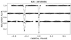 |
Fig. 1. Sample light curves of KIC 3858884 after detrending. The light curves have been folded within one orbit and shifted vertically by 0.27 from each other for illustrative purposes. The first three observed orbits are shown. Only every 12th data point is drawn for better visibility. |
3. Disentangling the light curve
Due to the strong interdependence of the eclipse and pulsation characteristics there is no reliable method yet to simultaneously fit the eclipses and the pulsations to the data. Although it would be tempting to use, for example, wavelet-based algorithms to automatically fit the pulsations during a binary modelling as red noise or Gaussian processes and remove them in one step, they have not been tested for cases of eclipse-modulated pulsations. Besides, they would probably have difficulty in handling hundreds of simultaneous pulsations. Rather, we carried out a traditional iterative procedure of separating the eclipsing binary signal, consisting of the light contributions of the equilibrium surface brightness maps of the stars, and the pulsation signals. The methods analysing eclipse-modulated pulsations operate on the pulsation-only signal, while of course also relying on the binary model, to be determined from the binary signal.
Maceroni et al. (2014) started their iterative procedure with cleaning the pulsations identified from the harmonic analysis of the data outside the eclipses, then binary modelling, followed by harmonic analysis of the full data range, and repeating the last two steps until convergence. Each of these steps operates on the residuals of the previous step. We followed the same procedure, with a few differences. (i) We started with the eclipsing binary (EB) modelling of folded and binned data together with the pulsations, using the parameters determined by Maceroni et al. (2014) as initial values; (ii) All pulsations were treated as pure sinusoidal signals, until the binary parameters stopped improving; (iii) Peaks that were multiples of the orbital frequency were considered as residuals from an incomplete binary modelling, their signals collected and transferred from the pulsation data to the EB data; (iv) After convergence was achieved in 4 iterations, all but the 8 largest frequencies were subtracted as radial modes modulated on the secondary, by being multiplied by the secondary’s normalised contribution to the integrated flux, as derived from the binary model, while the 8 largest modes were fitted with an EM reconstruction described in Sect. 5.2.2. Using this result we performed a final, fifth iteration to refine the parameters. This step proved to be a significant improvement, since the bulk of the pulsation signal is contained in these frequencies. It resulted in a dramatic reduction of the residuals in the last iteration, as illustrated in Fig. 2.
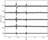 |
Fig. 2. Evolution of the residuals for KIC 3858884 across the five iterations of the light curve disentangling process, from top to bottom. All points from the full dataset are plotted. The centres of the two eclipses are marked with vertical dashed lines. |
We omitted the undetermined modes of the rest of pulsations because they do not not impact this analysis. The only exceptions are probably the hidden modes which have small amplitude when uneclipsed but large amplitude during the eclipses. However, we neglected them during the disentangling, because the achieved residuals suggested that only a few such modes may present.
All modes were assumed on the secondary because the diminishing of the residuals during the secondary eclipses indicated so, at least for the largest amplitudes. This was the conclusion of both Maceroni et al. (2014) and our investigation detailed in Sect. 4 regarding the sources of the individual pulsations.
3.1. Enhancing the binary model
We used the PHOEBE code (Prša & Zwitter 2005) for fitting the binary model. For this purpose the current light curve data were folded within one orbit, and binned with a resolution of 0.0005 between in the phase intervals [ − 0.25, −0.21] and [ − 0.14, 0.14] covering the eclipses, and 0.005 elsewhere. The binning also yielded formal point to point errors which were used during the fit.
As initial parameters for the binary model fitting, we used the binary solution determined by Maceroni et al. (2014). and the adjusted parameters were: the inclination i, the surface potentials Ω1, 2, the eccentricity e, and the argument of periastron ω. All the other values were kept at their values of the initial solution. In particular, we had no reasons trying to readjust quantities that had already been determined from spectroscopic data by Maceroni et al. (2014). The gravity darkening and albedo coefficients were kept fixed at their theoretical values for radiative envelopes (g = 1, A = 1, von Zeipel 1924). The limb darkening coefficients of a square root law corresponding to the Kepler transmission function were set to be internally interpolated by PHOEBE for the given atmospheric parameters.
The derived binary parameters are presented in Table 1, compared with the previous result of Maceroni et al. (2014) as reference. Our results are quoted with one more decimal digit in order to make it clear that all of them were fitted, and not adopted.
Orbital and geometric parameters of KIC 3858884.
The values differ from the reference values more than the quoted errors in the latter; we think the reason lies in the different handling of the modulated pulsations (radial versus mapped modes). Our primary reason was the removal of the binary signal with the highest possible accuracy – better than the amplitude of the pulsations to be mapped; otherwise the residuals would be regarded as modulation signal and totally distort the mode mapping results. Errors in the geometric quantities are better tolerated by the mapping algorithms (Bíró & Nuspl 2011). For this reason we did not attempt to derive uncertainties for the determined parameters.
3.2. Extraction of pulsation frequencies
In analysis, we generally report the frequencies in units of orbital frequency, forb = 0.0385 d−1. In Table A.1 (on Zenodo; see the Sect. Data availability), the frequencies are also listed in units of c/d.
The harmonic analysis of the current pulsation signal was repeated at every iteration as part of the disentangling procedure. The data were the residuals after the current binary signal was interpolated to the original light curve points and subtracted. The original data consisted of 358 240 points, corresponding to a Nyquist frequency limit of 19 082 forb, (735 d−1). We did an initial analysis on the original dataset with full time resolution in order to check for the highest frequency signal present. It was found that there is no peak in the Fourier spectrum above 580 forb (22.3 d−1). Therefore, we undersampled the data by 20, that is, we kept every twentieth point, to reduce the unnecessarily high time resolution. This lowered the number of points to 17 912 and reduced the Nyquist limit to 750 forb (29 d−1). The undersampling does not affect the frequency resolution which is proportional to the inverse of the total time base of the dataset, as it is fR ∼ 0.036 in our case.
Both the primary and secondary eclipses have been excluded from the harmonic analysis in this section. Their presence cause more trouble than the periodic gaps due to their masking – real side peaks around the frequencies of all modulated pulsations versus side peaks in the spectral window; the latter is already affected by the large gap of 15 months between Q2 and Q8 anyway. However, when the locations of the individual modes were investigated (Sect. 5.2), we performed additional harmonic analyses with exactly the same configuration, but with primary or secondary eclipses also being involved.
We used SigSpec (Reegen 2007) to detect and extract the frequencies from the data. It is an automated program which operates on the basis of probabilistic formulation of signal detection, and selects peaks based on their spectral significance. We adhered ourselves to the usual threshold of S/N = 4, which corresponds to a significance limit of ∼5.47 (Reegen 2007), even though, as noted by Maceroni et al. (2014), the real useful limit for the present data is probably as high as 12. Our choice was driven by the desire to obtain a disentangling as perfectly as possible, taking into account every signal, but not belonging to the eclipses.
As a precaution and convenience in observational asteroseismology, we applied a classic filtering mechanism in order to select the real pulsation frequencies. One consequence of nonlinear processes in stellar pulsations is the appearance of combination frequencies of the form
 (1)
(1)
where fi and fj are the parent frequencies, ci and cj are integer numbers and Δf is the Rayleigh frequency resolution, the inverse of the time base of the full dataset (Pápics 2012). We wrote a Python script to search for such combinations in the list of the detected frequencies. Table A.1 (on Zenodo; see the Sect. Data availability) lists the properties of the first 55 peaks with the largest amplitude together with the detected frequency combinations.
4. Identification of the source stars of the pulsations
The performance of mode identification relies on the fact that the right frequencies are modelled on the right stars. In this regard, there is some controversy among the published results about KIC 3858884. Maceroni et al. (2014) concluded that at least the strongest pulsations are most likely originate on the secondary, indicated by the behaviour of the residuals in the Rossiter-McLaughlin effect and in the light curve cleaned from pulsations. On the other hand, Manzoori (2020) argued that the two largest pulsations of similar frequency and amplitude (cf. Table A.1; on Zenodo; see the Sect. Data availability) are the fundamental modes of the two similar components, and provided support by computing time delays for the two pulsations, using the phase modulation method of Murphy et al. (2014; hereafter PM), showing oppositely varying phases for the two pulsations (Appendix B of cited work). If they are indeed the fundamental modes, it seems logical to assume that they originate from two stars with similar physical properties.
Figure 3 shows the residuals of the light curve at various stages, folded with the orbital period. The top panel displays the pulsation signals after the subtraction of the EB model. The diminishing of the pulsation amplitudes during the secondary eclipses is evident. There is also some modulation going on during the primary eclipse phases, but is less pronounced. The bottom panel displays the residuals after also subtracting all the pulsations, but as pure harmonic signals, without any modulation anywhere. Therefore, the more real modulation is going during an eclipse, the larger its residuals are. It is clear that if F1 and F2 were fundamental radial modes of two different stars, then the observed pulsations would experience modulations of comparable magnitude at the two eclipses. Yet, we see a very pronounced effect during the secondary eclipses and a very small one during the primary one.
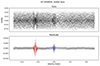 |
Fig. 3. Residuals of KIC 3858884 folded with the orbital phase. Top: After subtracting the binary model. Bottom: After also subtracting all the pulsations modelled as pure, uneclipsed sinusoidal signals. Blue and red mark the sections affected by the primary and secondary eclipses, respectively. Only every second data point is plotted, for a better visibility. |
We experimented exclusively with the locations of F1 and F2. For this, we got rid of all the other pulsations as unperturbed harmonic signals. Then we subtracted also F1 and F2 under all possible variants of their location, and compared the residuals. Figure 4 shows the results. Whenever either frequency is assumed on the primary, the residuals increase dramatically. The lowest residuals are attained when both are modulated on the secondary (bottom plot in the Fig. 4).
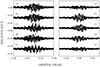 |
Fig. 4. Residual investigation for identifying the sources of F1 and F2. All the other frequencies were subtracted as unperturbed sinusoidals. From top to bottom: (a) – both F1 and F2 are also sinusoidals; (b) – both are on the primary; (c) – F1 on primary, F2 on secondary; (d) – reverse of (c); (e) – both are on the secondary. |
The above findings still do not exclude that one of the two pulsations is on the primary: it could be different from a radial mode, thus causing more subtle modulations, as illustrated in Fig. A.1 (on Zenodo; see the Sect. Data availability). Manzoori (2020) used the phase modulation method to prove that F1 and F2 show phase variations of opposite sign. To clear up the issue, we have also performed a PM analysis. The classical method, which works in the time domain, without the knowledge of the orbital period, found periodic phase variations for F1 and F2 that were running together, but with a period different from the known orbital period. Therefore, we changed to the orbital phase domain with the known period, and sliced the times series into smaller segments according to the orbital phase rather than time. The rationale was that there may be other stellar or non-stellar processes influencing the fit of the initial phases; however, our main aim is only to determine the sources of the frequencies. The eclipse phases were omitted from the analysis in order to avoid the complications related to modulated pulsations. We then fitted the first eight frequencies constraining their frequencies and out of eclipse amplitudes, adjusting the phases only. The modified method met our expectations, we could obtain firm evidence that F1 and F2 are indeed coming from the secondary component (see Fig. 5). For these frequencies, the obtained time delays are in fair agreement with the theoretical values, which were computed from line-of-sight distances modelled by second generation of PHOEBE (Prša et al. 2016). As for the other frequencies, the results were inconclusive, probably due to their lower amplitudes.
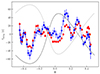 |
Fig. 5. Time delays of F1 and F2 computed with the modified phase modulation method (see text for the details). The blue and red filled circles correspond to F1 (f = 187.65 forb) and F2 (f = 193.95 forb), respectively. The continuous and dotted grey lines show the theoretical time delays of the primary and secondary components, respectively, which were computed from line-of-sight distances modelled by the second generation of PHOEBE (Prša et al. 2016). |
Finally, we performed a so-called double EM of the first eight frequencies, where mode pulsations on both stars are mapped simultaneously, using the data from both eclipses. If a pulsation is assumed on a star, but has no associated modulations in the dataset during the eclipses of that star, then its surface pattern is expected to receive a negligible power. Therefore, we assigned the same 8 frequencies to both the primary and secondary, and let the mapping procedure decide about their proportions on each star in terms of amplitude. Because the emphasis was on the separation of the modulations rather than providing sensible pulsation maps, no symmetry was assumed at all about the solutions ; instead, a most uniform solution was sought. The amplitudes of each reconstructed pattern, computed outside the eclipses, are shown in Table 2, and indicate that the majority of the most dominant modes, including F1 and F2, come from the secondary component, although the disambiguation becomes less reliable when going towards the weaker modes. In fact, F9 and F10 may as well reside on the primary. We note in passing that F9 is the almost exact double of F10, so the two pulsations may indeed have a common origin, suggesting the presence of some nonlinear modes as well.
Result of the double eclipse mapping for KIC 3858884.
In our opinion, the results (see Table 3) of the above detailed investigations provide a firm evidence that F1 and F2, as well as most of the significant pulsations, are located on the secondary star. There is also some evidence that the five of other dominant frequencies are identified to be from the secondary, and the one with the lowest amplitude (F10) among them from the primary star.
Pulsation source analysis for the KIC 3858884 system.
5. Mode identification
5.1. Methods
In the linear adiabatic approximation the surface pulsation patterns of the oscillation eigenmodes of a spherically symmetric star can be described in terms of surface spherical harmonic functions Yℓm(θ,φ) in the coordinate system tied to the symmetry axis of the star (Cox 1980). The two numbers ℓ (degree) and m (azimuthal order) are the two surface mode numbers identifiable with various photometric or spectroscopic techniques. Rotation and tidal interaction cause distortions in the amplitude distribution of these eigenmodes in addition to frequency splittings (Aerts et al. 2010), leading to equatorial concentration (Reese et al. 2009) or mode trapping (Handler et al. 2020), among others. Therefore, the use of spherical harmonics may not always be appropriate or justifiable. Nevertheless, for the study of intrinsic stellar oscillations in binaries where these perturbing effects are small, they can still be a useful approximation. In accordance, we employed two approaches in modelling the surface patterns. The first, the dynamic eclipse mapping (DEM) method, reconstructs general surface pulsation patterns with the possibility to impose certain symmetry properties on them, from which the mode numbers can be inferred either by topological resemblance or by quantitative analysis of the amplitude and phase profiles. The second, direct fitting (hereafter DF), works with the usual surface spherical harmonics as basis functions, and looks for the best matching set of mode numbers either by sequential probing of all possible cases, or by a stochastic sampling of their parameter space. It also has the potential to detect a possibly tilted pulsation axis, which cannot be excluded in such a wide binary system.
Both methods rely on the assumption that the resulting time-dependent surface pattern can be approximated by the linear superposition of the individual oscillating patterns. For small amplitude pulsations this is the usual assumption made by all other analysis approaches too, on the basis that small changes in the local temperature can be added up linearly, and also induce a linear change in the local brightness around its value determined by the equilibrium value of the local effective temperature at first approximation. Also, they were constructed to only study intrinsic pulsations in binaries, free from tidal locking or trapping. Although future extensions could make these cases partially tractable, it is beyond the scope of our paper.
5.1.1. Eclipse mapping
Eclipse mapping2 (EM) is an image reconstruction technique originally conceived for mapping the brightness distributions of accretion discs in eclipsing cataclysmic binaries (Horne 1985) and later in more regular systems (Collier Cameron 1997). Eclipse events are effectively sampling the surface of the star undergoing the eclipse, convolving its surface brightness distribution into the eclipse light curve. Eclipse-mapping methods employ regularised inversion techniques to restore the brightness distribution from the light curve.
Bíró & Nuspl (2011) constructed a variant of EM extended to reconstruct periodic time-dependent surface patterns, primarily pulsations. For every involved frequency it furnishes two maps, the so-called ‘cosine’ map A⋅ cos ϕ and its ‘sine’ counterpart, A⋅ sin ϕ, leading to amplitude and phase maps A and ϕ. The convolution causes a significant loss of information on the patterns themselves; however, with reasonable assumptions about their nature, in terms of symmetries, they can be restored to an extent that allows mode identification through the analysis of their the nodal line structure. The assumption is that the amplitude depends on the co-latitude only; similarly the phase depends on the longitude only, and linearly. This approach also allows for deviations from the spherical harmonics caused by rotational distortion. Since its original implementation, the DEM algorithm has received a significant improvement: the use of a hidden image space, connected to the real image space via a fuzzy pixel-based intrinsic correlation function. This separation of regularisation and correlations led to a dramatic improvement in the smoothness and reliability of the reconstructed patterns, which previously rendered the method awkward for real applications.
Both the application of symmetry requirements and the inference on the mode numbers require the knowledge of the symmetry axis, fixed in space. In close or moderately wide systems it is customary to assume an orbitally aligned rotation axis, to which the pulsations are aligned, unless there is evidence indicating otherwise, e.g from the Rossiter-McLaughlin effect (Albrecht et al. 2009). In wide systems like KIC 3858884 the validity of this assumption is less certain. Fortunately, the Direct Fitting method has the potential to estimate an orientation from the pulsation data.
5.1.2. Direct fitting
In addition to eclipse mapping, Bíró (2013) also reported on another algorithm termed direct fitting (DF), which models the surface patterns explicitly as spherical harmonics Yℓm(θ,φ) defined in a coordinate system tied to the symmetry axis of the pulsation. For a mode with known ℓ, m, the only free parameters are its amplitude and phase. If its out of eclipse amplitude and phase in the integrated flux as determined from time series analysis are applied as additional constraints, even these are uniquely determined, and the problem reduces from a fit to a simple evaluation of the match between synthetic light curves and data, for all reasonable modes (ℓ,m). The idea is to test all possible partitionings of the modes, up to a certain maximum ℓ, and select the combination giving the best fit to the data. However, as the number of simultaneous modes increases, the number of combinations to be tested also increases as (ℓ+1)2N, where N is the number of frequencies and ℓ stands for the maximum degree, which makes the process computationally challenging. For example, for 8 frequencies and degrees up to ℓ = 3 it would mean more than 4 billion cases to investigate.
There is an existing semi-solution, which is a variant of DF. The algorithm is similar to a method in time series analysis known as frequency whitening, just performed with Yℓm-s, calling hence DFCLEAN in the following. The idea is to search for the best fit per frequencies instead of simultaneously on all frequencies, while the unknown ones are kept as radial and the identified ones with determined (ℓ,m) mode numbers. Although the search is way faster in that way than the DF, this algorithm probe much lower number of possible nonradial mode configurations.
To overcome this issue, we developed a program which performs a MCMC search using DF as its core program (Bókon & Bíró 2020, YLMCMC). A simple Metropolis-Hastings algorithm is used for sampling. The modes are treated as categorical variables, discrete variables with special ordering. After experimentation, the best ordering of the modes proved to be according to the deviation of their modulation curve – in the context of the investigated binary model – from that of the radial mode (0,0), in terms of the sum of square of the residuals (χ2).
In our runs, the mode degree was limited to ℓ ≤ 3. Modes with larger ℓ have such large cancellations that they are invisible outside the eclipses and are therefore undetected. The starting point of the Markov chain was in every run the all-radial modes case, and all modes are assigned uniform prior probabilities. The resulting joint posterior probability distribution of ℓ and m parameters for all modes is then used to draw conclusions.
The modelling with spherical harmonics also opens up the possibility of inferring a most plausible value for the pulsation axis, being the polar axis of the coordinate system in which the pulsation patterns can be described as spherical harmonics. As with EM, DF also requires the knowledge of this axis when fitting individual modes. However, when a spherical harmonic is viewed from another coordinate system with a different polar axis, it can be described as the linear combination of all spherical harmonics of the same degree ℓ, defined in the new system:
 (2)
(2)
where  are the elements of the Wigner rotation matrix which is a function of the Euler rotation angles α, β and γ of the transformation from the current system to that of the pulsation axis. α is the azimuth of the axis, clockwise from the meridian facing the observer and around the orbital axis; β is its tilt from the orbital axis; the phase shift mγ of the third angle is incorporated as a common phase shift of all the Yℓm′ components, and does not appear explicitly in the analysis. Therefore it is possible in principle to infer a best estimate of the pulsation axis in two steps. First a set of ℓ-multiplets
  is assumed for each pulsation, and the DF procedure now partitions various ℓ-s. Then the Wigner coefficients of all modes are solved for a common value of α, β via a numerical optimisation. Tests performed in Bíró (2013) were encouraging, showing that the orientation of the pulsation axis may be recoverable even in the presence of rotationally distorted modes.
The road map of analysis is then as follows. First a DF of multiplets is performed to estimate the obliquity of the pulsation axis. The derived orientation of the axis is then used, first to perform EM, which furnishes reconstructed surface patterns and allows estimates for mode numbers; another DF of single modes is then performed to infer mode numbers in the frame of the spherical harmonics model. The comparison of the two sets of mode numbers may shed light on deviations of the pulsation patterns from spherical harmonics, or point to limits of capability of the method for the particular binary system.
There is a limit on the number of simultaneously mappable modes, as revealed by tests performed previously by Bíró & Nuspl (2011). Single modes can be successfully reconstructed even from a single sampled eclipse. Multiple modes require multiple eclipses in order to be properly separated during the mapping. As a rule of thumb, it was found that, for reasonably precise data like those from space telescopes, the number of simultaneously restorable modes will not be larger, possibly even less, than the number of the eclipses involved. Larger noise in the data can be compensated by collecting observations of more eclipses.
The algorithms were also found to be less reliable when more than a half dozen modes were present and some pulsations had much smaller amplitudes than others. In this case, the smaller amplitudes tend to be improperly reconstructed. To deal with this shortcoming, we analysed the pulsations in groups or packets of roughly similar orders of amplitude, in decreasing order. All the modes to be mapped were temporarily cleaned as radial modes with uniform amplitude and phase patterns, affected only by decreasing variation of their amplitudes proportional to the fractional contribution of their host star to the integrated flux; in our study, all the studied modes were located on the secondary component. All the modes already mapped were properly subtracted with their fitted modulations.
5.2. Results
Once the origins of the frequencies were clarified, the actual mode-identification task could begin.
For the mapping procedures the data were resampled to uniformly spaced points with more amenable resolution in time. They covered the secondary eclipses and some of their surrounding out of eclipse portions. The same set of points in terms of the fractional photometric phase was used for all the individual eclipses. This speeds up the mapping procedures: an eclipse kernel covering a single secondary eclipse can be replicated for all the eclipses, shifting its temporal factors properly in time. Quadratic interpolation was sufficient for the resampling, given the density of the original data points. Each section was covered by 801 points from −0.28 to −0.18 in orbital phase. This covers the secondary eclipses between −0.25 and −0.23 as well as two additional sections on the two sides; the latter are included to constrain the uneclipsed amplitude and phase characteristics of the modes to be fitted. The 11 secondary eclipses contained in the data are thus covered by 8811 individual data points.
We first attempted this for the frequencies listed in Table 3, omitting the combination frequencies. A DF in multiplet mode yielded angles α ∼ 32° and β ∼ 30° for the symmetry axis. However, both the EM and DF runs were essentially unsuccessful, regardless of whether all the frequencies were handled together, or grouped in 4+4 according to similar amplitudes, or cleaned one by one using DF. The achieved fits to the data were only marginally better than the all-radial case. In the case of the EM, tightening the fit in terms of the sum of squared residuals (χ2) only increased the noise in the images but did not reduce the residuals in the eclipse phases, signalling that the algorithm is fitting noise rather than structure. For reference, the runs were repeated with perfectly aligned pulsation axis, with the same result.
This called for a more thorough investigation regarding which modes are really involved in the modulations. The nature of the residuals pointed to the possible presence of unaccounted hidden modes contaminating the data. These are modes with surface patterns that yield nearly perfect mutual cancellation outside the eclipses, but get amplified during the eclipses due to the symmetry breaking. (1,0), (2,1) or (3,1) are such modes when viewed nearly edge-on, like in the present system.
Fortunately, the amount and quality of the short cadence data for KIC 3858884 allowed us to search in the frequency spectra for modes affected by the eclipses. Eclipses modulate the amplitudes of the individual pulsation modes with the periodicity of the orbital motion, resulting in the development of side peaks around the frequency of the affected mode, with spacing equal to the orbital frequency, forb. Tidal perturbations also induce frequency splitting with the same spacing, although there were cases where the excited pulsations were close to the harmonics of the orbital frequency (Bowman et al. 2019) instead of the splitting of the actual frequencies. However, the splittings of tidal origin are present in all types of datasets, while the eclipse-related modulations only occur if the respective eclipse phases are included in the analysis.
Following this logic, we performed two additional SigSpec runs on datasets extended to include either the primary or the secondary eclipses, respectively, using the same sampling and program setup as before, except that a lower value of 3 was used for the significance threshold in order to detect as many side peaks as possible. We refer to the original list of peaks obtained from the data excluding all eclipses (Sect. 3.2) as ‘noe’, and the two new lists of peaks as ‘pri’ and ‘sec’.
The peaks were then examined on échelle diagrams with the folding frequency of forb. Figure 6 shows the two diagrams for the ‘pri’ and ‘sec’ cases, together with the peaks common to all three spectra. We also cross-identified the peaks across the three cases. In doing so, we took the Rayleigh frequency fR ≈ 0.036 as a reference value for the precision of the peak frequencies, although the matching of the peaks turned out to be much tighter, within about one-fourth of the quoted precision, in agreement with the heuristic results of Kallinger et al. (2008) that the precision also depends on the significance of the peak.
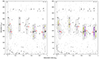 |
Fig. 6. Échelle diagrams of pulsation frequencies with respect to the orbital frequency, extracted from the data including primary eclipses (left panel) and secondary eclipses (right panels). Grey filled circles mark the individual frequency peaks intrinsic to the actual dataset. Peaks common to all the three datasets are shown with the bold diagonal squares. The numbered peaks are those for which a significant amount of side peaks were found in either of the cases. The side peaks are colour coded according to the ratio of their amplitudes to that of their central peak: ratios lower than 5% are shown in yellow, the larger ones in violet. (The threshold only serves visualisation purposes). All symbol sizes are proportional to their amplitudes on a logarithmic scale. The boxes show the regions in which side peaks were searched for; their widths is equal to the fR (∼0.036), and extend vertically by 60 forb in both directions. Only F10 was found to have significant modulation during the primary eclipses. The dotted box centred on 0 shows the location where orbitally resonant frequencies and remnants of an incompletely subtracted binary signal are expected. |
It is intriguing to see the very low level of modulations related to the primary eclipses. Only a few peaks show notable side peaks in the ‘pri’ spectra: F10 and perhaps F13 and F4, but the latter two are blended with F1 and F2. The secondary eclipses, as expected, modulate a larger number of modes and more strongly, namely F1 and F2 as expected, then F3, F6 and F15, and, unexpected from previous evidence, F44 and F52. Figure C1 shows the modulations of these modes computed by adding up their main peaks and side lobes. F44 and F52 clearly have the characteristics of hidden modes, their amplitudes increasing dramatically during the secondary eclipses, reaching levels equal to the residuals from the first unsuccessful mappings.
Thus from the échelle diagrams we updated the set of frequencies to be mapped on the secondary: F1, F2, F3, F6, F15, F44, and F52. Their characteristics are replicated in Table 4 from the main frequency table in the appendix for easier reference.
Final set of frequencies selected for mode identification.
We generated artificial modulated pulsations for all spherical harmonic modes with ℓ up to and including 3, using the current binary parameters and the same time points as used for the time series analyses above. The first frequency F1 = 187.65 forb was used for all modes. No noise was added. We then performed SigSpec runs on these noiseless data to locate the first 100 peaks in the frequency range 100–300 forb. The simulated data and their spectra are shown in Figs. A.1 and A.2 (on Zenodo; see the Sect. Data availability). The structure of side peaks is clearly visible for all cases. They are shown for positive m-s only; for negative m they are mirrored around the central peak. (They appear on the panels of modulated light curves, though.) We experimented with the number of peaks, required to be included, in order of decreasing amplitude, to reproduce the modulated signals to an acceptable accuracy. We found that at least 80 peaks were required for a good approximation.
For comparison, we located the side peaks of the modulated frequencies using the ‘sec’ échelle diagram. In this procedure, the matching tolerance was lowered to 1/4 fR to exclude close but unrelated peaks. Also, to avoid any spurious peaks and especially those of possible tidal origin, only peaks present exclusively in the ‘sec’ spectrum were considered as candidates. The side peaks and their resulting modulated pulsations are shown in Fig. C1 in a similar manner as for the simulated data.
The number of detected side peaks from the real data with noise is much lower than from the simulations. Therefore a meaningful isolation of the individual modulations based on their detected side peaks is beyond possible, even for these extraordinarily precise data. Instead, one can go the other way around: subtract the signals of all the peaks of the ‘sec’ spectrum from the data, except the target peaks and their side lobes. We note that the peaks in ‘sec’ already describe the modulations during the secondary eclipses, and therefore they should be interpreted as unmodulated harmonic signals.
5.2.1. Direct fitting
First, we performed a DF of ℓ-multiplets to estimate the orientation of the symmetry axis. The first five modes were used for this purpose3. The best solution, with χ2 = 1.48, yielded the ℓ-numbers (1, 1, 2, 2, 2) for the five frequencies. The fitting of Wigner coefficients on the best parameters gave α = 21.9° and β = 21.6° for the orientation of the rotation axis. This is very close to an aligned configuration. The associated mode numbers turned out to be (1, 0), (1, 0), (2,−1), (2, 0) and (2, 1). This came as a surprise, given that modes (1,0) are hidden modes.
To check the validity of these mode numbers, we performed runs of DF, DFCLEAN, and YLMCMC, all in singlet mode. Table 5 summarises the results. Generally speaking, there is a good agreement in the mode numbers found by these runs with fixed axis, but they differ significantly from those given by the free axis algorithm. We have two conjectures regarding the cause of this disagreement. It could happen if the pulsation patterns cannot be appropriately described by spherical harmonics – although we think it unlikely for nearly spherical stars on such a wide orbit corresponding to the nearly 26 days period, even if it is eccentric. Or the remnants of the many other unfitted modes, taken into account as uniform patterns affected by the eclipses, are disturbing the data sufficiently so that sensible information on the orientation of the axis cannot be inferred. All the analyses have been repeated for an aligned axis case (α = 0°, β = 0°). The results are shown in Table 6.
Results of direct fitting for the α = 22° and β = 22° configuration.
Mode identification from the performed reconstruction for the selected frequencies.
5.2.2. Dynamic eclipse mapping
As with DF, we proceeded with the EM analysis in two consecutive steps, with the two sets of frequencies grouped according to similar amplitudes. In EM, the goodness of fit to the data is user-specified in terms of the χ2 value. If only white noise is present and its level is correctly estimated, χ2 = 1, or a slightly larger value is appropriate. For white noise of unknown level a noise scaling is possible by tuning χaim2 so that the value of a related, so-called R-statistics, proposed by (Baptista & Steiner 1993) as a measure of the correlation between adjacent residuals, becomes close to zero. Unfortunately this approach rarely works in practice due to the presence of additional contaminating factors, like the remnants of modulations of the many smaller amplitude pulsations. Some experimenting is required regarding the smallest value of attainable χ2 without significant distortions in the maps. The first version of EM as described in Bíró & Nuspl (2011) was very sensitive to noise, which easily propagated into the maps as unrealistic, noisy patterns as the level of fit was being tightened. The introduction of the hidden space solved this shortcoming, allowing only maps that are smooth on the scale of the resolution of the hidden space, which is covered typically by about 50 uniformly distributed vertex points. As a consequence, they are more immune to noise in the data.
There will be a lower limit of χ2 below which the algorithm cannot go, giving at that point a smooth map, which, however, is unfeasible in the sense that it is far from the expected ‘rosette’ symmetry of the pulsation patterns with a symmetry axis. Also, given that many different modes are bound to cause nearly the same modulation, as illustrated in Fig. A.1 (on Zenodo; see the Sect. Data availability) for the case of the secondary eclipses of KIC 3858884, as our aimed χ2 was being pushed down, the solutions kept switching between the various nearly equivalent modes (e.g. (0,0),(1,±1),(2,±2) are such a group), separately for each mapped mode. Selecting an appropriate χ2 then unavoidably injects a certain amount of subjectivity into the solution. More precise data and, more importantly, less correlated noise would certainly help in resolving this ambiguity. In the present case, we tried to mitigate the subjective factor by first going for the smallest attainable χ2 value, and then relaxing it until the maps become feasibly. It was comforting to see that at least the signs of m remained consistent for each map throughout the iterations. We note that the values of χ2 attained by DF results can only serve as upper limits for EM, because they assume the more restrictive spherical harmonics.
The reconstructed maps and their amplitude and phase profiles are shown in Fig. C2. Contrary to our expectations, neither of the two strongest signals (F1, F2) emerged as radial mode. Both were mapped as sectoral modes: (2,−2) for F1 and (3,3) for F2, respectively. These mode numbers are unfortunately not recovered by the DF runs. We discuss the possible causes for all frequencies in the next section. On the other hand, F3 and F15 were reconstructed as radial modes. DF runs also unambiguously attributed (0,0) to them.
F6 was reconstructed as a sectoral mode (1,−1). In comparison, DF failed to recover it, yielding equivalent modes instead: (0,0), (1,1), (2,0). F44 and F52 were identified as (3,−1) and (2,1), respectively. These are typical hidden modes, showing the most pronounced modulations during the secondary eclipses. Because they are more distinguishable from the other modes in terms of their modulation pattern, DF procedures essentially gave the same results, but sometimes with opposite sign for m.
The fit to the data achieved by the EM reconstructions is shown in Fig. C3. It shows the joint result of the two split, 5+2 runs. Figure C4 illustrates the contributions of the individual modes to the integrated flux for a single eclipse, as synthesised from the reconstructed maps.
6. Discussion and conclusions
We invested a considerable amount of effort into identifying the source components of the pulsations, given that the previous two works on this system (Maceroni et al. 2014; Manzoori 2020) came to conflicting conclusions in this regard. Maceroni et al. (2014) obtained the first binary model from Kepler photometry and extensive supplementary spectroscopy. These authors identified the high-frequency p mode oscillations, which contain most of the power, and also low-frequency g mode oscillations. No evidence was found for tidal perturbations of the g modes. Similarly, faint signs of orbital modulation were found for some peaks, and no rotational splitting was detected. From the study of clustering of the p mode frequencies (Breger et al. 2009), Maceroni et al. (2014) found it plausible that of the two strongest modes, F2 is a radial mode and F1 is a non-radial counterpart in the same cluster, provided that both pulsations originate from the secondary component. The common origin was supported by the behaviour of both the photometric and RV residuals from their EB analysis with respect to the orbital phase: the scatter intensifies during the secondary eclipse in both cases.
However, Manzoori (2020), while performing an extensive tidal oscillation analysis on the system, concluded that F1 and F2 reside on different stars, on the grounds that they are very similar, as are also the stars, and therefore it is plausible that F1 and F2 are their radial mode frequencies. This conclusion appears to be supported by the values of the pulsation constant Q = Ppuls (ρ/ρ⊙) (Breger 1979, Table II) for these frequencies as second and third overtones of the radial mode based on the stellar masses and radii derived by Maceroni et al. (2014). In further support of this conclusion, Manzoori (2020) presents results of the phase-modulation method of Murphy et al. (2014) applied to the data, confirming periodic time-delay variations in opposite phase for the two frequencies.
Our results, however, do no support this scenario. Similar to Maceroni et al. (2014), we find that the behaviour of the residuals from the EB analysis, and after having subtracted all the identified pulsation frequencies as pure sinusoidals (Fig. 3), shows without doubt that most of the eclipse modulations take place during the secondary eclipse. There is clearly some modulation during the primary eclipse as well, indicating that some low-amplitude frequencies indeed do originate from the primary star. However, if the two dominant modes were on separate stars, the residuals would be amplified to similar extents during the two eclipses, having similar geometry for an orbit seen nearly side-on (with ω ∼ 22°). We do not see this in the data. In addition, an eclipse mapping of the first eight frequencies simultaneously on both stars attributed most of the modes to the secondary, leaving only F9 and F10 with a possible primary origin. We note that F9 is approximately two times F10. We also note that the time delays of about ±500s of Manzoori (2020, Fig. B1) seem to be much larger than those expected from the binary orbit, which should vary between 116s and 132s depending on the orientation of the orbit, and is about ±120s for the current configuration. The period of variation as assessed from the figure also seems to be too large compared to the orbital period. In any case, we find that applying phase-modulation methods to multi-mode pulsations with many concurrent modes is not straightforward. Our attempt to apply such a method in the traditional way showed the delays of the two signals to vary synchronously rather than oppositely, but with an uncertain period. A folded version of the PM technique, using the known orbital period, only marginally reproduced the time-delay curves expected for the current orbit, and the two delays still run together, as shown in Fig. 5.
We now turn to a discussion of the mode identification results. A full pulsation analysis is beyond the scope of this paper, and one has already been carried out in detail in previous works (Maceroni et al. 2014; Manzoori 2020). Here we focus on assessing the feasibility of the various EM methods regarding the mode identification. These methods use the surface sampling phenomenon of the mutual eclipses, and depend on the orbital parameters of the binary system and basic stellar parameters, such as radii and limb darkening coefficients only; they therefore provide independent information for future asteroseismic investigations. We also did not attempt to map the very low-amplitude g modes, as they would have challenged the methods beyond their capabilities.
The échelle diagram folded with the orbital frequency proved to be a crucial diagnostic tool in identifying the peaks modulated during the eclipses. Of the p modes, we successfully located seven such candidates on the secondary star. These are however not the seven strongest amplitude pulsations. We possibly found one candidate (F10) on the primary as well, but with less certainty. A direct fitting (DF) method using multiplets was applied to the first five candidates in order to determine the orientation of the symmetry axis, and resulted in α ∼ 22° and β ∼ 22° for the azimuthal and tilt angles, suggesting an aligned configuration. We then performed generic DF analyses in both tilted and aligned configurations for the same five candidates. Their results mostly agree, giving the same mode numbers, or equivalent mode numbers that are barely distinguishable in the present eclipse geometry. Therefore, we assumed an aligned configuration for the subsequent runs, and repeated the DF procedures for all seven frequencies.
We also successfully reconstructed surface pulsation patterns with EM, and inferred best-matching mode numbers. The two strongest modes were found to be sectoral, with (2,−2) and (3,3) for F1 and F2 according to EM. It came as a surprise that none of them appear to be radial. In turn, F3 and F15 were found to be best approximated by radial modes in all mapping procedures involving various symmetry angle orientations. The pulsation constant for F3 is Q = 0.026, which in theory can be attributed to the first overtone of the fundamental radial frequency of the secondary (Breger 1979, Table II) – although, according to Maceroni et al. (2014), both stars have evolved considerably from the main sequence, and so it is not clear whether the classical pulsation constant can serve as a useful diagnostic in this case. Regarding F15, we note that it may be a combination frequency, such as F15 ≈ 3 ⋅ F12 − 3 ⋅ F8 (Table A.1; see the data availability section), in which case its radial nature is no surprise. F6 is best described by a retrograde sectoral mode (1,−1). F44 and F52 are two hidden modes that surfaced during the échelle diagram analysis; our initial ignorance of them hampered our first set of mappings, but after their discovery, not only did the analysis succeed, but they could also be identified as (3, ±1) and (2, ±1). We should mention however that the reconstructed pattern for the latter is less reliable. It can also be noted that all the surface patterns suffer from distortions arising from the interplay of the different frequencies, which is a consequence of the small number of individual eclipses covered by the data compared to the number of mapped modes (11 eclipses for 7 frequencies).
In general, we were able to uniquely determine the absolute value of m, but not its sign. The results from EM have systematically opposite signs compared to the DF results. Figure A.1 (on Zenodo; see the Sect. Data availability) shows that, for the geometric configuration of KIC 3858884, modes with identical ℓ but oppositely signed m are close to each other in terms of their modulations; therefore they can be mistaken for each other. If the quality of the data allows it, the investigation of the associated side lobe structure may help to resolve this ambiguity: the main peak is seen centered for m = 0 and shifted to the left or right for m < 0 and m > 0, respectively. A visual check of Fig. C1 shows that the main peak of F1 is located left of the maximum of the side lobe forest, while for F2 it is shifted to the right, supporting the values of m found from EM rather than DF. Unfortunately, our capacity to carry out such a check quickly reduces with decreasing amplitude. For F3, there is a marginal hint of centered location, that is, m = 0, which is indeed the value derived from all mappings; for F6, the peak appears left-shifted, pointing to a negative m. For F15, the structure is too sparse to draw a conclusion, and for the two ‘hidden’ modes, the absence of additional side lobe ‘islands’ prevents a clear conclusion (cf. Figure A.1, lower panels; see the data availability section).
Regarding those leading pulsations that do not seem to be modulated at all, such as F4, F5, F7, F8, and F9, most of them are recognised as combination frequencies (cf. Table A.1; on Zenodo; see the Sect. Data availability), and therefore they are not real peaks and are not expected to contribute to the modulations.
It is not clear why the DF and EM results disagree for F1 and F2, while they mostly match for the other modes, including the two low-amplitude tesseral modes F44 and F52. Although the radial and the low-order sectoral modes give rise to similar modulations, one would expect the strongest signals to be the most clearly differentiated. This discrepancy may be a result of the fact that these modes are the most different from spherical harmonics due to their larger amplitudes. The other source of disagreement could be that the direction of the pulsation axis, as inferred from the photometric modulations, is poorly determined. In our opinion, this is causing the greatest hinderance to further progress.
As a final conclusion, we successfully located seven pulsations on the secondary component, including the two strongest ones. Their modulations were detected in the frequency spectra of datasets with one or both types of eclipse masked out. Crucial to this detection was the use of échelle diagrams. We also successfully identified these modes using DF and EM methods. We were able to uniquely determine the radial mode of the secondary as F3. To our knowledge, this is the first time that hidden modes have been found and identified.
We feel that our analysis reveals only a fraction of the vast potential of EBs with pulsating components, and in particular this system, KIC 3858884, with its superb short-cadence Kepler photometry data. As pointed out already by Maceroni et al. (2014), a future spectroscopic survey of the system could be a tremendous help for mode identification. Apart from improving the atmospheric parameters and opening the way for spectroscopic mode identification methods, spectra of sufficient resolution and signal-to-noise ratio could also provide the possibility to fix the orientation of the symmetry axis –which is currently the largest source of uncertainty in our photometry-based analysis– using the Rossiter-McLaughlin effect.
Data availability
The figures (Figs. A.1, A.2 and B.1) and the table (Table A.1) of Appendices A and B are available at https://doi.org/10.5281/zenodo.14178674.
We are aware that there is some divergence in using the term ‘eclipse mapping’ across the scientific community; some communications use it to name the phenomenon itself, others refer to the reconstruction method. We follow the tradition of the first papers on the topic, and use the term to name the reconstruction method.
A seven-frequency run was also completed, giving similar results, but its follow-up validation with almost 300 million combinations of individual modes would have taken too much time, and was therefore abandoned.
Acknowledgments
We would like to thank the anonymous referee for all the recommendations and remarks to improve the manuscript. We would like to thank László Molnár and Susmita Das for the discussions of possible asteroseismologic implication regarding δ Scutis and for their modelling efforts. This work was supported by the PRODEX Experiment Agreement No. 4000137122 between the ELTE Eötvös Lóránd University and the European Space Agency (ESA-D/SCI-LE-2021-0025). This project has been supported by the LP2021-9 Lendület grant of the Hungarian Academy of Sciences. This project has received funding from the HUN-REN Hungarian Research Network. I.B.B acknowledges the financial support of the Hungarian National Research, Development and Innovation Office – NKFIH Grant K-147131. This paper includes data collected by the Kepler mission. Funding for the Kepler mission is provided by the NASA Science Mission directorate.
References
- Aerts, C. 2021, Rev. Mod. Phys., 93, 015001 [Google Scholar]
- Aerts, C., & Eyer, L. 2000, ASP Conf. Ser., 210, 113 [NASA ADS] [Google Scholar]
- Aerts, C., Christensen-Dalsgaard, J., & Kurtz, D. W. 2010, Astron. Astrophys. Libr., 848, 866 [Google Scholar]
- Albrecht, S., Reffert, S., Snellen, I. A. G., & Winn, J. N. 2009, Nature, 461, 373 [Google Scholar]
- Auvergne, M., Bodin, P., Boisnard, L., et al. 2009, A&A, 506, 411 [NASA ADS] [CrossRef] [EDP Sciences] [Google Scholar]
- Balona, L. A., & Evers, E. A. 1999, MNRAS, 302, 349 [NASA ADS] [CrossRef] [Google Scholar]
- Baptista, R., & Steiner, J. E. 1993, A&A, 277, 331 [NASA ADS] [Google Scholar]
- Bíró, I. B. 2013, EAS Publ. Ser., 64, 331 [Google Scholar]
- Bíró, I. B., & Nuspl, J. 2011, MNRAS, 416, 1601 [CrossRef] [Google Scholar]
- Bókon, A., & Bíró, I. B. 2020, Bulg. Astron. J., 33, 47 [Google Scholar]
- Bowman, D. M., Johnston, C., Tkachenko, A., et al. 2019, ApJ, 883, L26 [Google Scholar]
- Breger, M. 1979, PASP, 91, 5 [NASA ADS] [CrossRef] [Google Scholar]
- Breger, M., Lenz, P., & Pamyatnykh, A. A. 2009, MNRAS, 396, 291 [NASA ADS] [CrossRef] [Google Scholar]
- Briquet, M., & Aerts, C. 2003, A&A, 398, 687 [NASA ADS] [CrossRef] [EDP Sciences] [Google Scholar]
- Chen, X., Ding, X., Cheng, L., et al. 2022, ApJS, 263, 34 [CrossRef] [Google Scholar]
- Collier Cameron, A. 1997, MNRAS, 287, 556 [NASA ADS] [CrossRef] [Google Scholar]
- Cox, J. P. 1980, Theory of Stellar Pulsation (PSA-2) (Princeton University Press) [CrossRef] [Google Scholar]
- Dupret, M. A., De Ridder, J., De Cat, P., et al. 2003a, A&A, 398, 677 [NASA ADS] [CrossRef] [EDP Sciences] [Google Scholar]
- Dupret, M. A., Scuflaire, R., Noels, A., et al. 2003b, Ap&SS, 284, 129 [NASA ADS] [CrossRef] [Google Scholar]
- Eze, C. I., & Handler, G. 2024, ApJS, 272, 25 [NASA ADS] [CrossRef] [Google Scholar]
- Fuller, J., Kurtz, D. W., Handler, G., & Rappaport, S. 2020, MNRAS, 498, 5730 [NASA ADS] [CrossRef] [Google Scholar]
- Gamarova, A. Y., Mkrtichian, D. E., Rodriguez, E., Costa, V., & Lopez-Gonzalez, M. J. 2003, ASP Conf. Ser., 292, 369 [Google Scholar]
- Garrido, R. 2000, ASP Conf. Ser., 210, 67 [NASA ADS] [Google Scholar]
- Gaulme, P., & Guzik, J. A. 2019, A&A, 630, A106 [NASA ADS] [CrossRef] [EDP Sciences] [Google Scholar]
- Guo, Z., Fuller, J., Shporer, A., et al. 2019, ApJ, 885, 46 [Google Scholar]
- Handler, G., Kurtz, D. W., Rappaport, S. A., et al. 2020, Nat. Astron., 4, 684 [Google Scholar]
- Horne, K. 1985, MNRAS, 213, 129 [NASA ADS] [Google Scholar]
- Johnston, C., Tkachenko, A., Van Reeth, T., et al. 2023, A&A, 670, A167 [NASA ADS] [CrossRef] [EDP Sciences] [Google Scholar]
- Kallinger, T., Reegen, P., & Weiss, W. W. 2008, A&A, 481, 571 [NASA ADS] [CrossRef] [EDP Sciences] [Google Scholar]
- Kjeldsen, H., & Bedding, T. R. 1995, A&A, 293, 87 [NASA ADS] [Google Scholar]
- Koch, D. G., Borucki, W. J., Basri, G., et al. 2010, ApJ, 713, L79 [Google Scholar]
- Kurtz, D. W. 2022, ARA&A, 60, 31 [NASA ADS] [CrossRef] [Google Scholar]
- Liakos, A., & Niarchos, P. 2017, MNRAS, 465, 1181 [NASA ADS] [CrossRef] [Google Scholar]
- Maceroni, C., Lehmann, H., da Silva, R., et al. 2014, A&A, 563, A59 [NASA ADS] [CrossRef] [EDP Sciences] [Google Scholar]
- Manzoori, D. 2020, MNRAS, 498, 1871 [Google Scholar]
- Mkrtichian, D. E., Kusakin, A. V., Gamarova, A. Y., & Nazarenko, V. 2002, ASP Conf. Ser., 259, 96 [NASA ADS] [Google Scholar]
- Murphy, S. J., Bedding, T. R., Shibahashi, H., Kurtz, D. W., & Kjeldsen, H. 2014, MNRAS, 441, 2515 [Google Scholar]
- Nuspl, J., Biro, B. I., & Hegedus, T. 2004, ASP Conf. Ser., 318, 350 [NASA ADS] [Google Scholar]
- Pápics, P. I. 2012, Astron. Nachr., 333, 1053 [CrossRef] [Google Scholar]
- Prša, A., & Zwitter, T. 2005, ApJ, 628, 426 [Google Scholar]
- Prša, A., Conroy, K. E., Horvat, M., et al. 2016, ApJS, 227, 29 [Google Scholar]
- Reed, M. D., Brondel, B. J., & Kawaler, S. D. 2005, ApJ, 634, 602 [NASA ADS] [CrossRef] [Google Scholar]
- Reegen, P. 2007, A&A, 467, 1353 [NASA ADS] [CrossRef] [EDP Sciences] [Google Scholar]
- Reese, D. R., MacGregor, K. B., Jackson, S., Skumanich, A., & Metcalfe, T. S. 2009, A&A, 506, 189 [NASA ADS] [CrossRef] [EDP Sciences] [Google Scholar]
- Reyniers, K., & Smeyers, P. 2003a, A&A, 409, 677 [NASA ADS] [CrossRef] [EDP Sciences] [Google Scholar]
- Reyniers, K., & Smeyers, P. 2003b, A&A, 404, 1051 [NASA ADS] [CrossRef] [EDP Sciences] [Google Scholar]
- Ricker, G. R., Winn, J. N., Vanderspek, R., et al. 2015, J. Astron. Telescopes Instrum. Syst., 1, 014003 [Google Scholar]
- Rodríguez, E., & Breger, M. 2001, A&A, 366, 178 [NASA ADS] [CrossRef] [EDP Sciences] [Google Scholar]
- Rodríguez, E., López-González, M. J., & López de Coca, P. 2000, A&AS, 144, 469 [CrossRef] [EDP Sciences] [Google Scholar]
- Shi, X.-D., Qian, S.-B., Li, L.-J., & Liao, W.-P. 2021, MNRAS, 505, 6166 [NASA ADS] [CrossRef] [Google Scholar]
- Shi, X.-D., Qian, S.-B., & Li, L.-J. 2022, ApJS, 259, 50 [NASA ADS] [CrossRef] [Google Scholar]
- Szatmary, K. 1990, J. Am. Assoc. Var. Star. Obs., 19, 52 [NASA ADS] [Google Scholar]
- von Zeipel, H. 1924, MNRAS, 84, 665 [NASA ADS] [CrossRef] [Google Scholar]
- Welsh, W. F., Orosz, J. A., Aerts, C., et al. 2011, ApJS, 197, 4 [Google Scholar]
- Zhou, A. Y. 2014, Pulsating Components in Binary and Multiple Stellar Systems- A Catalog of Oscillating Binaries [Google Scholar]
Appendix C: Additional figures
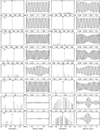 |
Fig. C1. The modulations of selected frequencies, as determined from their sidelobes identified in the ‘pri’ and ‘sec’ spectra involving primary or secondary eclipses, respectively. Every row contains data for one frequency, marked in the leftmost panels. From left to right: columns 1 and 2 – data (peaks + their synthetic signals) for primary eclipses; columns 3 and 4 – same for secondary eclipses. We note that the peak amplitudes in the frequency spectra are plotted on a nonlinear – square root – scale in order to make the smallest peaks visible. Black upside down triangles mark the central peaks. Dashed vertical lines in the light curve panels (columns 2 and 4) mark the eclipse regions. |
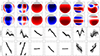 |
Fig. C2. Result of eclipse-mapping reconstruction. Each column contains maps and profiles for the frequency labelled at the top of the column. The top two rows contain the reconstructed maps as seen by the observer and the corresponding ‘reference map’ holding the “rosette” symmetry content of the former. The uniformly grey polar caps represent the uneclipsed regions, the integrated signals of which were fitted by additional virtual pixels. Row 3 (from top) shows the amplitude profile in function of the stellar co-latitude, with north on the left (0 degrees) and south to the right (180 degrees). Row 4 shows the phase profile in function of the stellar longitude, from −180 to +180 degrees. Longitude 0 at the centre corresponds to the stellar meridian. The individually computed values for the pixels are plotted with grey symbols, and the values interpolated from the fitted model to the same locations are plotted in black. The axis ticks are drawn every 90 degree, except for the vertical axis of the amplitude profiles. The tick labels have been omitted from the graphs to save space. The horizontal dashed lines in the amplitude graphs mark the individual zero levels. |
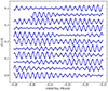 |
Fig. C3. The fit of the combined eclipse-mapping reconstructions to the data. Data for the individual orbital cycles are shown in separate rows from bottom to top. The input data are shown as grey circles, the fitted model as blue curves. |
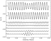 |
Fig. C4. The individual flux contributions of the maps reconstructed by eclipse mapping. The curves, labelled by their frequencies, are shown on the same scale, only shifted vertically by arbitrary amounts. |
All Tables
Mode identification from the performed reconstruction for the selected frequencies.
All Figures
|
Fig. 1. Sample light curves of KIC 3858884 after detrending. The light curves have been folded within one orbit and shifted vertically by 0.27 from each other for illustrative purposes. The first three observed orbits are shown. Only every 12th data point is drawn for better visibility. |
| In the text | |
|
Fig. 2. Evolution of the residuals for KIC 3858884 across the five iterations of the light curve disentangling process, from top to bottom. All points from the full dataset are plotted. The centres of the two eclipses are marked with vertical dashed lines. |
| In the text | |
|
Fig. 3. Residuals of KIC 3858884 folded with the orbital phase. Top: After subtracting the binary model. Bottom: After also subtracting all the pulsations modelled as pure, uneclipsed sinusoidal signals. Blue and red mark the sections affected by the primary and secondary eclipses, respectively. Only every second data point is plotted, for a better visibility. |
| In the text | |
|
Fig. 4. Residual investigation for identifying the sources of F1 and F2. All the other frequencies were subtracted as unperturbed sinusoidals. From top to bottom: (a) – both F1 and F2 are also sinusoidals; (b) – both are on the primary; (c) – F1 on primary, F2 on secondary; (d) – reverse of (c); (e) – both are on the secondary. |
| In the text | |
|
Fig. 5. Time delays of F1 and F2 computed with the modified phase modulation method (see text for the details). The blue and red filled circles correspond to F1 (f = 187.65 forb) and F2 (f = 193.95 forb), respectively. The continuous and dotted grey lines show the theoretical time delays of the primary and secondary components, respectively, which were computed from line-of-sight distances modelled by the second generation of PHOEBE (Prša et al. 2016). |
| In the text | |
|
Fig. 6. Échelle diagrams of pulsation frequencies with respect to the orbital frequency, extracted from the data including primary eclipses (left panel) and secondary eclipses (right panels). Grey filled circles mark the individual frequency peaks intrinsic to the actual dataset. Peaks common to all the three datasets are shown with the bold diagonal squares. The numbered peaks are those for which a significant amount of side peaks were found in either of the cases. The side peaks are colour coded according to the ratio of their amplitudes to that of their central peak: ratios lower than 5% are shown in yellow, the larger ones in violet. (The threshold only serves visualisation purposes). All symbol sizes are proportional to their amplitudes on a logarithmic scale. The boxes show the regions in which side peaks were searched for; their widths is equal to the fR (∼0.036), and extend vertically by 60 forb in both directions. Only F10 was found to have significant modulation during the primary eclipses. The dotted box centred on 0 shows the location where orbitally resonant frequencies and remnants of an incompletely subtracted binary signal are expected. |
| In the text | |
|
Fig. C1. The modulations of selected frequencies, as determined from their sidelobes identified in the ‘pri’ and ‘sec’ spectra involving primary or secondary eclipses, respectively. Every row contains data for one frequency, marked in the leftmost panels. From left to right: columns 1 and 2 – data (peaks + their synthetic signals) for primary eclipses; columns 3 and 4 – same for secondary eclipses. We note that the peak amplitudes in the frequency spectra are plotted on a nonlinear – square root – scale in order to make the smallest peaks visible. Black upside down triangles mark the central peaks. Dashed vertical lines in the light curve panels (columns 2 and 4) mark the eclipse regions. |
| In the text | |
|
Fig. C2. Result of eclipse-mapping reconstruction. Each column contains maps and profiles for the frequency labelled at the top of the column. The top two rows contain the reconstructed maps as seen by the observer and the corresponding ‘reference map’ holding the “rosette” symmetry content of the former. The uniformly grey polar caps represent the uneclipsed regions, the integrated signals of which were fitted by additional virtual pixels. Row 3 (from top) shows the amplitude profile in function of the stellar co-latitude, with north on the left (0 degrees) and south to the right (180 degrees). Row 4 shows the phase profile in function of the stellar longitude, from −180 to +180 degrees. Longitude 0 at the centre corresponds to the stellar meridian. The individually computed values for the pixels are plotted with grey symbols, and the values interpolated from the fitted model to the same locations are plotted in black. The axis ticks are drawn every 90 degree, except for the vertical axis of the amplitude profiles. The tick labels have been omitted from the graphs to save space. The horizontal dashed lines in the amplitude graphs mark the individual zero levels. |
| In the text | |
|
Fig. C3. The fit of the combined eclipse-mapping reconstructions to the data. Data for the individual orbital cycles are shown in separate rows from bottom to top. The input data are shown as grey circles, the fitted model as blue curves. |
| In the text | |
|
Fig. C4. The individual flux contributions of the maps reconstructed by eclipse mapping. The curves, labelled by their frequencies, are shown on the same scale, only shifted vertically by arbitrary amounts. |
| In the text | |
Current usage metrics show cumulative count of Article Views (full-text article views including HTML views, PDF and ePub downloads, according to the available data) and Abstracts Views on Vision4Press platform.
Data correspond to usage on the plateform after 2015. The current usage metrics is available 48-96 hours after online publication and is updated daily on week days.
Initial download of the metrics may take a while.