| Issue |
A&A
Volume 693, January 2025
|
|
|---|---|---|
| Article Number | A263 | |
| Number of page(s) | 12 | |
| Section | Cosmology (including clusters of galaxies) | |
| DOI | https://doi.org/10.1051/0004-6361/202451803 | |
| Published online | 23 January 2025 | |
Turbulent pressure support in galaxy clusters
Impact of the hydrodynamical solver
1
Universitäts-Sternwarte, Fakultät für Physik, Ludwig-Maximilians-Universität München, Scheinerstr. 1, 81679 München, Germany
2
Astronomy Unit, Department of Physics, University of Trieste, via Tiepolo 11, I-34131 Trieste, Italy
3
INAF – Osservatorio Astronomico di Trieste, via Tiepolo 11, I-34131 Trieste, Italy
4
ICSC – Italian Research Center on High Performance Computing, Big Data and Quantum Computing, via Magnanelli 2, 40033 Casalecchio di Reno, Italy
5
Center for Computational Astrophysics, Flatiron Institute, 162 Fifth Avenue, New York, NY 10010, USA
6
Departament d’Astronomia i Astrofísica, Universitat de València, C/Doctor Moliner 50, E-46100 Burjassot (València), Spain
7
Max-Planck-Institut für Astrophysik, Karl-Schwarzschild-Straße 1, 85741 Garching, Germany
⋆ Corresponding author; fgroth@usm.lmu.de
Received:
5
August
2024
Accepted:
5
December
2024
Context. The amount of turbulent pressure in galaxy clusters is still debated, especially in relation to the impact of the dynamical state and the hydro-method used for simulations.
Aims. We study the turbulent pressure fraction in the intracluster medium of massive galaxy clusters. We aim to understand the impact of the hydrodynamical scheme, analysis method, and dynamical state on the final properties of galaxy clusters from cosmological simulations.
Methods. We performed non-radiative simulations of a set of zoom-in regions of seven galaxy clusters with meshless finite mass (MFM) and smoothed particle hydrodynamics (SPH). We used three different analysis methods based on: (i) the deviation from hydrostatic equilibrium, (ii) the solenoidal velocity component obtained by a Helmholtz-Hodge decomposition, and (iii) the small-scale velocity obtained through a multi-scale filtering approach. We split the sample of simulated clusters into active and relaxed clusters.
Results. Our simulations predict an increased turbulent pressure fraction for active clusters compared to relaxed ones. This is especially visible for the velocity-based methods. For these, we also find increased turbulence for the MFM simulations compared to SPH, consistent with findings from more idealized simulations. The predicted nonthermal pressure fraction varies between a few percent for relaxed clusters and ≈13% for active ones within the cluster center and increases toward the outskirts. No clear trend with redshift is visible.
Conclusions. Our analysis quantitatively assesses the importance played by the hydrodynamical scheme and the analysis method to determine the nonthermal or turbulent pressure fraction. While our setup is relatively simple (non-radiative runs), our simulations show agreement with previous, more idealized simulations, and represent a step closer to an understanding of turbulence.
Key words: turbulence / methods: numerical / galaxies: clusters: general / galaxies: clusters: intracluster medium
© The Authors 2025
 Open Access article, published by EDP Sciences, under the terms of the Creative Commons Attribution License (https://creativecommons.org/licenses/by/4.0), which permits unrestricted use, distribution, and reproduction in any medium, provided the original work is properly cited.
This article is published in open access under the Subscribe to Open model. Subscribe to A&A to support open access publication.
1. Introduction
The intracluster medium (ICM) of galaxy clusters is a very dynamic environment and is shaped by mergers, global gas motions, and turbulence (Carilli & Taylor 2002; Kravtsov & Borgani 2012). These processes act on different scales. Mergers and bulk motions directly impact the gas dynamics on large scales. Small scales, in contrast, are dominated by turbulent motions.
All of these gas motions can be described as different pressure terms contributing to the total pressure in the ICM. Besides gas motions, magnetic fields can also produce additional magnetic pressure. In combination, the aforementioned two contributions are often summarized as nonthermal pressure opposed to the thermal pressure of the gas.
In this work, we shall refer to the pressure due to small-scale turbulent motions as the turbulent pressure. The entirety of pressures except for the thermal, including turbulence, bulk motions, and possibly magnetic fields will be called nonthermal pressure.
A plethora of numerical and observational programs specifically target understanding the origin of the structure of the ICM. Turbulence is injected on large scales in merger shocks, after which it decays and cascades down to smaller scales (Roettiger & Burns 1999; Subramanian et al. 2006; Mohapatra et al. 2020, 2021). Both simulations and observations find that ICM turbulence is subsonic, with typical velocities of a few hundred kilometers per second (den Herder et al. 2001; Hitomi Collaboration 2016, 2018). For a sound speed on the order of cs = 1000 km/s, this results in a volume-filling Mach number between ℳ = 0.2 and 0.5, depending on the position within the clusters. While global measurements of turbulence in galaxy clusters can be understood within the context of the classical theory of subsonic turbulence that is supported by observations (e.g., the results by Hitomi Collaboration 2016, 2018), our understanding of its origin and dissipation scales still lacks a solid base.
Various X-ray observations provide an insight into ICM properties and aim to analyze ICM turbulence. Schuecker et al. (2004) quantified turbulence based on pressure fluctuations in the Coma cluster. They found that turbulence is described well by a Kolmogorov power spectrum, with an upper limit of the turbulent pressure that is 10% of the total pressure. Similarly, Zhuravleva et al. (2019) study density fluctuations from X-ray observations and quantify viscosity in the ICM. They derive velocities up to around a few hundred kilometers per second, closely following the expected Kolmogorov scaling for subsonic turbulence. Using spectroscopic lines with XMM-Newton, Gatuzz et al. (2023) confirm the Kolmogorov-like slope with driving scales of 10–20 kpc in Virgo.
Exploiting spectroscopically resolved lines to derive velocities, Hitomi Collaboration (2016, 2018) performed detailed measurements in the Perseus cluster, yielding velocities of between 100–200 km/s and a turbulent pressure support of only 4% compared to the total pressure. This value is at the lower end compared to many other results cited in this work. As Perseus also shows a cool core, it is often classified as relaxed in the center where the turbulence is measured, despite the cluster showing sloshing motions and an active galactic nucleus (AGN). As this is a single system, it is unclear from the aforementioned work if there is any dependence on the dynamical state. The result is still consistent with the upper limits of the spectroscopic measurements by XMM-Newton (den Herder et al. 2001) of 200–600 km/s.
An alternative method was used by Eckert et al. (2019). For the X-COP sample, they quantified the nonthermal pressure based on the deviation from hydrostatic equilibrium (HE) and found values between 2% and 15%, depending on the radius and cluster.
Different observations indicate that the amount of turbulence should depend on the dynamical state of the system. One indirect tracer of turbulence is the existence of a radio halo, which requires turbulent reacceleration. Cassano et al. (2010), Cuciti et al. (2015, 2021) found that merging systems typically host such a radio halo, while relaxed systems do not.
An alternative insight can be gained from simulations of cosmological boxes or zoom-in regions with adequate resolution. One main advantage is the access to the velocity data for every resolution element in the simulation. Nevertheless, it remains difficult to extract turbulence directly, as this requires a good estimate of the bulk flow.
Based on the velocity dispersion, Lau et al. (2009) found a turbulent pressure support of between 6–15%, increasing with radius, in relaxed systems and higher values of between 9–24% in unrelaxed systems. Using a slightly different approach – separating the smooth gas component from clumps, and computing median instead of mean properties – Zhuravleva et al. (2013) found consistent results. They found increased root-mean-square (rms) velocities in active clusters of ≈0.7 cs in units of the sound speed, compared to ≈0.4 cs in relaxed clusters.
In a series of papers, Vazza et al. (2009, 2012, 2017, 2018) have explored turbulence in galaxy clusters simulated with the ENZO code (Bryan et al. 2014) featuring adaptive mesh refinement (AMR; Berger & Colella 1989). They introduced the multi-scale filtering technique, which decomposes the total velocity into bulk and turbulent motions, predicting a turbulent pressure support of around 10%. In addition, they have shown a strong dependence on whether a constant or variable filtering length is used. Such a dependence is expected because the filtering length allows us to focus on motions only on the length scales defined by the size of turbulent eddies, ignoring any bulk motions on larger scales that can increase the kinetic energy budget.
Biffi et al. (2016) use a modern SPH implementation with a high-resolution shock-capturing method and a high-resolution entropy-increasing diffusion scheme (also known as artificial viscosity and conduction), with an additional stabilization of the method against the tensile instability using a high-order kernel for their simulations. They find overall high deviations from HE of around 10–20%, with a higher deviation for more disturbed systems. This is slightly higher than other values from previously quoted references in the introduction, but still consistent. In addition, not all of this deviation from HE will be attributed to turbulence; instead, this is only an upper limit.
A direct comparison between simulations and observations has been made by Sayers et al. (2021). Using the “Clump3d” method, they combined several observations to de-project the cluster and derive a nonthermal pressure based on the deviation from HE. Even when analyzed with the same method, simulations and observations show a significant disagreement in the nonthermal pressure fraction. It reaches ≈13% for simulations, while it is consistent with zero for observations. In addition, Sayers et al. (2021) find no dependence on the dynamical state.
Overall, the interpretation of the nonthermal pressure depends on the analysis method. Many strategies based on the deviation from HE include the effect of bulk motions, magnetic fields, cooling flows, turbulence, and everything not attributed to the thermal origin. Rotational patterns can also affect the nonthermal pressure support (Biffi et al. 2011). This makes the comparison between different results depend on subtleties and motivates the need for more robust methods. More direct methods such as the multiscale-filtering technique instead return the actual turbulent pressure, filtering out motions on larger scales.
Derived properties of ICM turbulence depend not only on the analysis method but also on the numerical setup. Detailed comparisons on different hydro-methods of simulating subsonic turbulence have mainly been made in idealized boxes (compare, e.g., Kitsionas et al. 2009; Price & Federrath 2010; Padoan et al. 2007; Bauer & Springel 2012; Price 2012). These works show that the power spectrum especially can be significantly impacted by the choice of hydro scheme.
In cosmological simulations, several works have studied the impact of individual numerical parameters. An overly high artificial viscosity can significantly reduce the amount of turbulence (Dolag et al. 2005). Also, artificial conductivity reduces turbulence, as a result of increased gas stripping (Biffi & Valdarnini 2015).
In this work, we want to extend the comparison of different hydrodynamical methods from idealized simulations to cosmological environments. In particular, we want to study the differences between meshless finite mass (MFM; Lanson & Vila 2008a,b) and smoothed particle hydrodynamics (SPH; Springel & Hernquist 2002) as two different hydro-methods on the resulting turbulence in the ICM. To this end, we use non-radiative, hydrodynamical zoom-in simulations of galaxy clusters as a clean setup that allows us to produce robust results to compare MFM and SPH. In addition, we want to quantify the impact of the analysis method, as well as of the dynamical state of the cluster.
The paper is organized as follows. In Sect. 2, we describe the code and simulation setup, followed by a description of the different methods used to analyze the simulations in Sect. 3. The general dynamical and thermodynamic properties of the clusters used in this work are described in Sect. 4. To gain an insight into the turbulence, we start with a general analysis of the velocity structure in Sect. 5, and present the resulting turbulent pressure support in Sect. 6. Our findings are discussed in Sect. 7 and we provide some outlook to possible future work in Sect. 8.
2. The simulations
2.1. OpenGadget3
The simulations were performed with the hydrodynamical cosmological simulation code OPENGADGET3. It was originally based on GADGET-2 (Springel et al. 2001; Springel 2005). Gravity was calculated with an octree particle mesh approach (Xu 1995; Springel 2005; Springel et al. 2021). Hydrodynamical forces were calculated either using modern SPH (Springel & Hernquist 2002) including artificial viscosity, as it is formulated by Beck et al. (2016a), and artificial conductivity, as it was formulated by Price (2008). Alternatively, the MFM hydro-solver was used, with the implementation presented by Groth et al. (2023).
Two hundred and ninety-five neighbors were used for the SPH calculations with a Wendland C6 kernel (Wendland 1995; Dehnen & Aly 2012), while only 32 neighbors with a cubic spline kernel (Monaghan & Lattanzio 1985) were best suited for MFM. This leads to an effectively higher spatial resolution for the hydrodynamical solver defined by the smoothing length, h, using MFM compared to SPH by a factor of ≈3. The SUBFIND substructure finder (Springel et al. 2001; Dolag et al. 2009) and a shockfinder (Beck et al. 2016b) were run on the fly.
2.2. Dianoga suite
We simulated seven massive galaxy clusters from the Dianoga suite of zoom-in regions (Bonafede et al. 2011). The background cosmological evolution follows a flat ΛCDM cosmology with Ωm = 0.24, Ωb = 0.04, h = 0.72, and σ8 = 0.8. The mass resolution is Mdm = 109 h−1 M⊙, Mgas = 1.6 ⋅ 108 h−1 M⊙. The gravitational softening corresponds to 3.75 h−1 kpc for gas and 11.25 h−1 kpc for DM particles.
All selected clusters have a mass larger than 1015 h−1 M⊙. Their names and masses are listed in Table 1.
List of some general properties of the galaxy clusters analyzed in this study.
The selection includes active clusters with high merger activity and relaxed clusters that undergo mainly smooth accretion or minor mergers. This diversity allows us to study the effect of the dynamical state and compare the results to other simulations and observations of populations of different clusters.
Every cluster was simulated twice: once with the MFM solver and once with SPH. The main properties such as R200 and M200 quoted in Table 1 are consistent between the methods. Also, the classification between active and relaxed systems including the fraction of their evolution that they stay active or relaxed does not change when different hydro-solvers are used. Overall, differences between the methods are ≲1% for all quantities, and thus the values cited in Table 1 are identical within the given accuracy. For each simulation, we created 46 snapshots from redshift z = 0.43 until redshift zero, which we used for time averaging and studying their evolution.
3. Analysis methods
3.1. Dynamical states
To classify the dynamical state of a galaxy cluster, we followed the method described by Cui et al. (2017, 2018). We used two complementary criteria, whereby clusters were classified as active if at least one of them was satisfied. The first criterion is based on the shift of the center of mass (com) with respect to the cluster center defined by the minimum potential, where active clusters have an offset of at least
In addition, clusters for which the mass in substructures exceeds

are considered active. The cluster was classified as relaxed if none of the criteria were satisfied. The minimum potential, as well as the mass enclosed in substructures, was found using SUBFIND (Springel et al. 2001; Dolag et al. 2009). The center of mass was calculated for all gas and dark matter (DM) particles within R2001 of the SUBFIND center.
Both criteria are directly related to major mergers. The first one aims to capture the offset and sloshing of the gas within the DM potential shortly after the merger. Massive substructures can also offset the global mass distribution. The second criterion detects the infalling halo of an ongoing merger more directly.
Alternative criteria to classify the dynamical state would be possible; for example, ones based on the virialization (compare, e.g., Cui et al. 2018). We found, however, that these closely follow the two criteria used in this work, such that they are sufficient to classify the dynamical state of the system.
3.2. Clump3d analysis
The first option to calculate the nonthermal pressure contribution closely followed the method described by Sayers et al. (2021). In the first step, the ellipticity of the gas and total matter distribution was calculated according to the framework described by Fischer et al. (2022), Fischer & Valenzuela (2023) to account for deviations from spherical symmetry. The derived axes were used to define an elliptical radial coordinate used in all the fits.
The global density profile of gas plus DM was fit with a Navarro-Frenk-White profile (Navarro et al. 1997). The gas density was fit with a modified beta-model, and its temperature with a modified broken power law (Vikhlinin et al. 2006). The total pressure was obtained from these fits using the HE equation:
The thermal pressure was calculated directly from the gas density, ρgas, and internal energy, ugas, of all particles as:

with an adiabatic index of γ = 5/3. We used 40 radial bins equally distributed in log space between 0.01 R200 and 1.1 R200 to compute these profiles, using a logarithmic mean over the particles within each bin. The nonthermal pressure is given by the deviation from the assumption of HE. It was computed as the difference between the total and thermal pressure, Pnt = Ptot − Ptherm, limited to values greater than zero. Finally, the time and cluster-to-cluster average was computed with the radial coordinate normalized to R200.
The nonthermal pressure derived from this method includes contributions from turbulence and bulk motions. Depending on which physics is included, it could also contain, for example, magnetic pressure. In addition, strong shocks after recent mergers could impact the derived nonthermal pressure.
3.3. Vortex analysis – Helmholtz decomposition
The second method of calculating the nonthermal pressure fraction uses the velocity data from the simulation more directly. In particular, the solenoidal component of the velocity is associated with turbulence, while compressive motions are associated with shocks and bulk motion, following the results of Vazza et al. (2017) who find that the solenoidal component of turbulence dominates. In principle, the solenoidal component also contains components of motions at larger scales. Nevertheless, it tends to be more isotropic, behaving more like an additional pressure contribution compared to the compressive part (mainly radial; cf. Figure 7 in Vallés-Pérez et al. 2021a). Also, compressive velocity components can be associated with turbulence, and the mixture between solenoidal and compressive can vary depending on the type and driving of turbulence (Federrath et al. 2010, 2021). These results have been found for supersonic turbulence. For subsonic turbulence within galaxy clusters, a predominance of the solenoidal component has been found (Ryu et al. 2008; Vazza et al. 2014, 2017; Wang & He 2024). Overall, the solenoidal component is only an indirect tracer of turbulence, and we shall compare the performance in more detail in the remainder of the paper.
We used the VORTEX-P code developed by Vallés-Pérez et al. (2024) to perform a Helmholtz-decomposition (Vallés-Pérez et al. 2021a). The total gas velocity was split into compressive and solenoidal components that were derived via a scalar potential, ϕ, and vector potential, A, respectively, leading to a unique decomposition,


The potentials were found as solutions to the elliptic partial differential equations,

Internally, VORTEX-P assigned the SPH data to an ad hoc set of nested AMR grids, with higher resolution in regions of higher particle number density, especially in the cluster center and within substructures. We ran the decomposition in a region of 50 h−1 Mpc that was sufficiently large to contain the virialized region of the main cluster and not be influenced by boundary effects. The base grid had a resolution of Nx = 128 and a maximum of nl = 6 refinement levels. Cells at any refinement level containing more than  particles were set to refine, producing a quasi-Lagrangian refinement. These settings result in a peak resolution of Δx6 ≈ 6 kpc, which is on the same order as the minimum smoothing length. A cubic spline kernel was used to interpolate the MFM simulations, while a Wendland C6 kernel was used for the SPH runs. Interpolations in the decomposition used the same neighbor number as in the cosmological simulation they were applied to. Further details on the setup of the cosmological simulations are provided in Sect. 2. The solenoidal velocity was then mapped back from the internal AMR grid to the original particle positions. This can introduce some smoothing and small errors, which are, however, of the same order as the errors involved in the initial grid assignment (see Vallés-Pérez et al. 2024, their Figures 2 and 3).
The turbulent pressure within 40 elliptical shells was calculated directly from the particle-based velocity data:
The thermal pressure was also obtained directly from the gas properties according to Eq. (4). The total pressure is the sum of both. All properties were calculated as the mass-weighted mean.
3.4. Vortex analysis – Multiscale filtering
Finally, VORTEX-P can also perform a Reynolds decomposition to split the bulk component of the velocity field from the turbulent contribution. Following the initial idea by Vazza et al. (2012, 2017), we performed a multiscale filtering approach. The details of the implementation and the extension of the method to AMR have been described by Vallés-Pérez et al. (2021b).
The outer scale of turbulence was constrained iteratively for each cell center. A lower bound, L0 = 3Δxl, depended on the local resolution of the ad hoc AMR grid (i.e., the refinement level, l). Then, the filtering scale was iteratively increased until the turbulent velocity converged, indicating that longer spatial scales around the given point no longer contained more kinetic energy, and hence the outer scale of the inertial range had been reached. To avoid divergent behavior at discontinuities, the iteration also stopped if a shocked cell with a Mach number of ℳ ≥ 2.0 entered the integration domain. The resulting filtered mean velocity corresponds to the bulk motion, such that the turbulent velocity remains as the difference between the total and filtered mean velocity. As for the solenoidal velocity, the filtered velocities were mapped back to the particle position.
This decomposition offers the most direct way of measuring the turbulent velocity. The turbulent pressure was calculated according to Eq. (8), replacing the solenoidal velocity with the filtered one.
4. Cluster properties
To better understand the set of clusters, we first analyzed some of their main properties. The projected gas density maps of two clusters that are representative of both more active and more relaxed clusters are shown in Fig. 1. Maps of the remaining clusters are shown in the Appendix. Overall, the galaxy clusters simulated with MFM have general properties that are similar to those of their analogous SPH version, by visual inspection. The same is true for the location of substructures, as the large-scale evolution is dominated by gravity. The accretion history of the gas is also almost identical, with only minor timing differences.
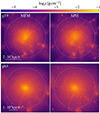 |
Fig. 1. Projected gas density maps for g19 and g63 as examples of one more active and one more relaxed cluster analyzed in this work at redshift z = 0. The dashed circle denotes Rvir. The upper maps have a size of Δx = Δy ≈ 3064 kpc h−1; the lower maps Δx = Δy ≈ 2797 kpc h−1. |
Differences are visible on smaller scales. Small structures tend to be destroyed earlier for MFM, leading to less substructures in the cluster. We do not find a statistically significant difference in the subhalo gas mass function between MFM and SPH within R200 of the cluster, as it is highly dominated by uncertainties in the substructure finder for such small halos. For MFM, we even find an overall higher number of subhalos. Nevertheless, SUBFIND struggles to find the gas content and the differences are minor when manually calculating the mass of the gas enclosed within the substructure. However, the smaller number of substructures in MFM simulations appears to be a consistent trend by visual inspection of all surface density plots. This observation is a sign that MFM mixes gas more efficiently and is more dissipative, which is consistent with more idealized simulations shown by Groth et al. (2023). In addition, from visual inspection, the diffuse volume-filling ICM appears to have more turbulent density fluctuations, visible mainly in the active cluster g19.
Cluster g19, classified as an active cluster at almost all redshifts, has more and larger substructures and ongoing mergers. In contrast, more relaxed clusters, such as g63, have fewer substructures and undergo mainly smooth accretion. Their overall shape looks much smoother and rounder.
The first panel shows the gas density, ρgas, the second panel the gas temperature in terms of kBT, and the third panel the entropy, S = T/ne2/3, profile. The electron density, ne, was calculated assuming full ionization. In the outskirts, the radial profiles shown in Fig. 2 are fully consistent between MFM and SPH. As was already visible in the maps, differences are present in the center. In particular, MFM tends to produce slightly cooler and denser cores compared to SPH. The central entropy is lower for MFM compared to SPH by a factor of ≈2, leading to the density being higher by a factor ≈2. This difference can be explained by MFM having more mixing and slightly higher numerical diffusivity, as is discussed by Groth et al. (2023) in the more idealized case of the hydrostatic sphere.
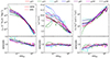 |
Fig. 2. Radial gas density, temperature, and entropy profiles for the clusters analyzed in this work at redshift z = 0. Lower panels show the ratio between MFM and SPH simulations for each cluster. |
Most of the clusters have a hot core that is visible both in temperature and in entropy. Only the g14 cluster has a cool core with a decrease in temperature in the center. This is most likely a transition state of the ongoing strong merger activity. In the surface density plot in Appendix B, even two distinct density peaks in the center are visible as a result of a recent major merger. This can significantly impact all radial profiles for this particular cluster.
The gas mass to halo mass relation for the different clusters evaluated inside different radii, R200, R500, and R2500, is shown in Fig. 3. The MFM and SPH simulations lead to almost identical results when evaluating the masses inside larger radii (i.e., R200 and R500), as the global structure does not change. The gas content roughly reaches the cosmological one, Ωb/Ωm ≈ 16.7%. Strong clustering in the cluster center can even lead to gas contents above the cosmological value observed for a few clusters.
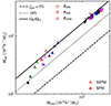 |
Fig. 3. Gas mass to halo mass relation for the clusters evaluated inside different radii at redshift z = 0. Lines indicate constant gas fractions, fgas. The colors of the clusters are the same as in Fig. 2. |
Slight differences appear in the innermost region inside R2500, where MFM generally leads to larger masses, consistent with the increase in density found in the radial profiles. The gas content ranges from 10% to approximately the cosmological value of 16.7%. While this is slightly larger than typical observation results of around 5–13% (Vikhlinin et al. 2006; David et al. 2012), differences can be explained by the absence of AGN feedback processes, which would reduce the gas fraction, especially at smaller radii (McNamara et al. 2000; Churazov et al. 2000; Eckert et al. 2021), and also star formation, which reduces the gas as it is transformed into stars.
The clusters show a variety of dynamical states, as is shown in Fig. 4. As is described in Sect. 3.1, clusters are classified as relaxed if both the offset of the center of mass and the mass enclosed in substructures are below the threshold marked by the gray-shaded region, while they are classified as active otherwise. Sloshing can make the center of mass approach the center defined by the minimum potential at some redshifts, but still have a nonzero relative velocity. Our second criterion of the mass enclosed in substructures ensures that the clusters can also be classified as active under such a condition.
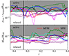 |
Fig. 4. Evolution of the center offset and substructure-mass over time of all clusters analyzed in this work. As is described in Sect. 3.1, a cluster is classified as relaxed only if both lines are below the two dotted thresholds, and otherwise as active. The colors of the clusters are the same as in Fig. 2. |
Some clusters, such as g14 (green) or g63 (purple), remain active or relaxed, respectively, at all redshifts. Other clusters, such as g55 (dark blue), can change their dynamical state over time, becoming active after larger mergers, but becoming relaxed again soon after.
There are only minor differences between the two hydro-methods. In particular, the mass enclosed in substructures is slightly smaller for MFM compared to that of SPH, but this does not change the dynamical state classification. Overall, using two criteria allows for a stable classification of the dynamical state.
5. Velocity structure
A more turbulent structure of the ICM for MFM compared to SPH is already visible from the surface density fluctuations. A more direct tracer is the velocity structure. In the upper part of Fig. 5, we show the solenoidal velocity component in a slice through the g55 cluster. As was expected, the global structure is qualitatively very similar between MFM and SPH. A strong increase can be found within a small region at the lower left. The total velocity shows that this region also has a very high infall velocity in general.
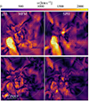 |
Fig. 5. Slice through the g55 cluster at redshift z = 0, showing the rotational component of the velocity in the upper panel and the multi-scale filtered velocity in the lower panel, each comparing MFM and SPH. The color indicates the absolute value of the solenoidal or filtered velocity, while the quivers show the direction. The dashed circle marks Rvir. |
Quantitatively MFM leads to higher velocities on average, and regions of large velocities are more extended. In addition, MFM has finer structures in the central region, which can be a result of a more turbulent structure and also the effectively higher resolution due to the smaller neighbor number.
The even more direct tracer for turbulence is the filtered velocity, shown in the lower panels of Fig. 5.
The patterns are similar to the solenoidal component, especially in the center. Nevertheless, the filtered velocity has a much lower maximum and does not show a strong increase within the accreting region. These differences persist and become clearer when averaging the absolute value within spherical shells, as is shown in Fig. 6.
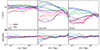 |
Fig. 6. Velocity profiles of all the simulated galaxy clusters, at redshift z = 0. The colors of the clusters are the same as in Fig. 2. The lower panels show the ratio between MFM and SPH simulations for each cluster. |
The differences between MFM and SPH are small, and substantial scatter between different clusters can be observed in the center. A mild increase on the order of 10% for MFM compared to SPH is visible on the outskirts of all panels, and is most pronounced for the filtered and solenoidal components. In the center, the differences are less obvious due to the strong scatter between different clusters, and within the scatter, it is consistent with all panels being identical between the hydrodynamical methods. More detailed conclusions can be drawn in Sect. 6.1, when also averaging over different redshifts studying the resulting pressure.
While turbulence is mainly solenoidal (compare, e.g., Vazza et al. 2017), other solenoidal motions can also be present in the ICM. Thus, the solenoidal component is a possible tracer of turbulence, but it tends to overestimate the turbulent velocity compared to the filtered one for almost every cluster. It is only an indirect tracer and should be used with caution. Nevertheless, as we shall see later, it still works reasonably well on average.
6. ICM turbulence
6.1. Turbulent pressure fractions
Finally, we can use the methods described in Sect. 3 to derive nonthermal or turbulent pressure fractions. We start by showing values at two individual redshifts, z = 0 and z = 0.33, in Fig. 7, to better compare to observations that typically cover a narrow redshift range.
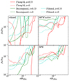 |
Fig. 7. Turbulent pressure profile averaged over all clusters at redshifts z = 0.33 and z = 0, comparing the three analysis methods: the clump3d method, the solenoidal velocity component, and the multi-scale filtered velocity. The sample is split between dynamical states (left column: relaxed, right column: active) and hydro-methods (top row: MFM, bottom row: SPH) used for the simulation. The linestyle indicates the redshift, the color the analysis method. As only seven clusters were used for averaging, a strong scatter between individual clusters dominates the uncertainty. |
A strong scatter is present as the number of clusters used for averaging is small. Only two of the clusters are relaxed at redshift z = 0, and five of them are active. Single outliers and timings of ongoing mergers can significantly influence the value. We find an increase in nonthermal pressure toward the outskirts, where the cluster is not in equilibrium but dominated by bulk, turbulent motions, and the presence of a larger number of substructures.
All the methods predict a nonzero turbulent pressure fraction for almost all clusters within most radial shells, with only a few exceptions. Due to the strong scatter, no clear differences are visible between the individual analysis methods. In addition, there are no clear trends for the turbulent pressure fraction with redshift. We find some increase in turbulent pressure for active clusters compared to relaxed ones; this seems to be even stronger for MFM compared to SPH. Relaxed clusters have on average only a few percent of turbulent pressure support, while active ones can have up to ≈20%. Nevertheless, these trends are not significant and all nonthermal pressure profiles are consistent within the strong scatter among individual clusters.
A clearer picture arises when averaging over redshifts 0.43 ≥ z ≥ 0, as is shown in Fig. 8.
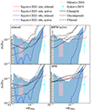 |
Fig. 8. Turbulent pressure profile averaged over all clusters and redshifts 0.43 ≥ z ≥ 0. The sample was split between dynamical states and hydro-methods used for the simulation, shown in the different panels. The solid line shows the results for the Clump3d analysis, the dashed line the pressure resulting from the solenoidal velocity component using the Helmholtz-decomposed velocity, and the dash-dotted line results from the multi-scale filtering. The typical uncertainty is on the order of σ = 0.08 and indicated for each method with an error bar on the left of each panel. |
We include different data from the literature as a comparison, including X-ray observations in the Perseus cluster (Hitomi Collaboration 2016, 2018), averages from the X-COP sample (Eckert et al. 2019), and the observations and the “300 simulations” (Cui et al. 2018) analyzed by Sayers et al. (2021). These span a wide range of possible turbulent pressure fractions, from Pnt/Ptot = 0 up to ≈0.13.
All the methods predict an increase on the outskirts located around 20 − 40% R200 m, consistent with the observations by Sayers et al. (2021), but stronger than for their simulation results. We typically find pressure values greater than zero, but still consistent with zero within the cluster-to-cluster and redshift-to-redshift scatter, which is typically around 0.08. The average 1σ scatter within 0.1 R200 for each method is indicated by a bar on the left of each panel.
For the relaxed clusters, we find turbulent pressure values smaller than the 300 simulations analyzed by Sayers et al. (2021) within the central region. Differences can be attributed to not including feedback processes in our simulations, which could potentially increase the amount of turbulence. Our results should thus be considered as lower limits. We find that the relaxed subsample is consistent with the spectral observations in the Perseus cluster (Hitomi Collaboration 2016, 2018), which is often assumed to be relaxed in the center, even though showing tracers of activity on the outskirts.
Active clusters yield higher turbulent pressure values that are more consistent with the simulations of the active clusters by Sayers et al. (2021). In general, our predictions, even though they do not include feedback processes, lie within the expected range of values found by other simulations and observations.
The clump3d method analyzing the deviation from HE predicts a nonthermal pressure of around ≲10%. It does not lie above the other two methods; rather, it lies below their predictions for MFM. This is opposed to the aim of the technique, which should indicate an upper limit for turbulence, as it also includes the nonthermal pressure contribution from bulk motions. A mild increase for active clusters compared to relaxed ones is present both for MFM and even stronger for SPH. Overall, the differences between hydro-methods are very small.
In contrast, the velocity-based methods show much clearer trends with the hydro-method and dynamical state. Interestingly, despite the radial velocity profiles showing a higher solenoidal velocity than the filtered one, we find the opposite trend for the pressure evaluated from the squared velocity. Nevertheless, the two methods produce very similar results. Relaxed clusters have a turbulent pressure fraction in the center of 2–4%. We find a strong increase in turbulent pressure for active clusters to 8–9% for SPH, and even higher up to 9–13% for the MFM simulation. Overall, we find small but non-negligible turbulent pressure fractions in all simulations, which are consistent with previous results.
6.2. Velocity distributions via line profiles
An alternative method of analyzing the distribution of velocities is via line profiles, which also offers a more direct comparison to observational results. We followed a simplified approach that was described by Dolag et al. (2005). When evaluating the line profile, the thermal broadening was ignored, and we focused purely on Doppler broadening due to velocity.
We assumed a constant iron abundance and emissivity proportional to the density, independent of temperature,
The total emission was computed as the sum of all particles, i, within the virial radius and a cylinder in the direction of the sightline in the z direction with a radius of r = 150 h−1 kpc,
The energy of the line was shifted due to the relativistic Doppler shift with βi = |vi|/c and the angle of the velocity with respect to the line of sight, cos ϕi = |vlos, i|/|vi|. As we neglected any thermal broadening, each individual line is described by a Dirac delta function, δ. The impact parameter was varied between 0, 250 h−1 kpc and 500 h−1 kpc in the x direction.
In Fig. A.1, we show the corresponding profiles binned at a resolution of 1 eV for a 6.702 keV iron line for all our clusters. As the density is highest in the center, the intensity of the line profile looking through the cluster center is the highest, and it decreases as the profile is evaluated moving further from the galaxy cluster center.
All line profiles are significantly broadened due to bulk- and turbulent motions by several tens of electronvolts. Their shape can vary between close to Gaussian to highly irregular profiles, depending on the velocity structure. Clusters g14, g19, and g55, which have the highest turbulent velocities in the radial profiles shown in Fig. 6, also show the broadest and most irregular line profiles compared to more relaxed clusters broadened by more than 50 eV.
Comparing the ratio of emissivity with MFM to SPH, we find that for many clusters this ratio increases toward the wings of the line, which indicates that the distribution is broader for MFM compared to SPH. In several cases, this can be seen even from the line profile itself. An exception is cluster g63, where a secondary maximum appears for SPH, but not MFM. This is most likely connected to a substructure at that position. Dolag et al. (2005) also argue that this method is highly sensitive to the timing and position of substructures.
Overall, the line profiles confirm the previous findings that more turbulence is present for MFM compared to SPH. Even if the line profile includes information not only on the turbulent motion but also on bulk velocities, it is a good tracer of turbulence.
7. Conclusions
We have analyzed the turbulent pressure support in galaxy clusters simulated with different hydro-methods, according to which the turbulence has been estimated in three different ways. Our set of zoom-in regions includes clusters at various dynamical states, so that even using few clusters we can get meaningful results.
The amount of turbulent pressure can vary significantly depending on the analysis method that was employed. The multi-scale filtering is the most direct approach, as it filters out bulk motions depending on the local structure. Like the filtered velocity, the solenoidal velocity is also a tracer of the turbulent velocity. Compared to the filtered velocity, it is slightly less direct and shows some differences in radial velocity profiles and derived turbulent pressure. Also, other solenoidal motions can be present, and turbulence can in principle also have compressive components, even though they are small in the ICM. Despite these limitations, we find that the solenoidal component follows the results based on the multi-scale filtered velocity reasonably well, especially considering that it is computationally much less expensive to calculate. While the clump3d method should predict an upper limit for the turbulence as it includes the effect of bulk motions, we find values similar to or even lower than those of the velocity-based methods. Possible explanations are limitations of the clump3d method, which relies on several assumptions, or that not all solenoidal or small-scale motion acts as an actual source of pressure for the HE equation. To unquestionably assess the reason for this discrepancy, a more detailed analysis beyond the scope of this paper is necessary.
Our setup allows us to compare hydro-methods of simulating turbulence in the ICM beyond idealized simulations, for the first time. The global structure is very similar between MFM and SPH, with differences on smaller scales. A visual inspection of the projected surface density reveals more small-scale density fluctuations for MFM compared to SPH. This can partly be explained by the effectively higher resolution for MFM, but also the better capturing of subsonic turbulence via the MFM scheme. Even though the reduced amount of small substructures for MFM is not statistically significant, this indicates more numerical dissipation and consequently more mixing for MFM.
Higher turbulent velocities are present for MFM than for SPH. Consistent with more idealized simulations, MFM predicts more turbulence for the velocity-based methods. For the clump3d method, only minor differences are present.
Finally, we analyzed the impact of the dynamical state. By exploiting velocity-based methods, we find that active clusters have more turbulence than relaxed ones, in contrast to Sayers et al. (2021). Some differences with respect to their work can be attributed to feedback processes, which are not present in our simulations as we instead preferred to have a clearer setup. Stellar and AGN feedback can drive feedback on small scales, increasing the overall amount of turbulence. While AGN feedback mainly affects the cluster in the center, the effect of stellar feedback can be more widespread. Although it does not include feedback processes, the amount of turbulence we find in our simulations is consistent with the range of values found in previous works between a few percent for relaxed clusters and up to ≈13% in the center for active clusters.
As the turbulent pressure increases toward the outskirts, the hydrostatic bias at the X-ray boundary around R500 ≈ 0.7 R200, where the signal is obtained by observations, is small, but non-negligible. We do not expect this result to change due to feedback processes. As a final remark, we stress that it is key to quantify what the discrepancies are between different simulations and analysis techniques, and why they arise: this allows us to understand their (possibly different) predicted nonthermal or turbulent pressure support.
8. Outlook
While this work focuses on a clean setup using purely hydrodynamical simulations, the inclusion of additional physical processes might partly change the picture. In particular, cooling would act as a sink for energy. Star formation, stellar, and AGN feedback, by contrast, would act as small-scale drivers of turbulence. As feedback processes self-regulate, they might also reduce differences between hydro-methods. More studies including feedback processes would be necessary to confirm our findings beyond non-radiative simulations. In addition, this could give a further insight into the expected amount of turbulence in real galaxy clusters.
The inclusion of magnetic fields would also provide an additional channel to study turbulence, as they closely couple via the dynamo effect. In addition, they can change the shape of turbulence and leave an imprint on the power spectrum.
Acknowledgments
We thank the anonymous referee for the constructive feedback which helped to improve the quality of this paper. FG and KD acknowledge support by the COMPLEX project from the European Research Council (ERC) under the European Union’s Horizon 2020 research and innovation program grant agreement ERC-2019-AdG 882679. MV acknowledges support by the Italian Research Center on High Performance Computing, Big Data and Quantum Computing (ICSC), project funded by European Union – NextGenerationEU – and National Recovery and Resilience Plan (NRRP) – Mission 4 Component 2, within the activities of Spoke 3, Astrophysics and Cosmos Observations, and by the INFN Indark Grant. UPS is supported by a Flatiron Research Fellowship at the Center for Computational Astrophysics (CCA) of the Flatiron Institute. The Flatiron Institute is supported by the Simons Foundation. FG, MV, and KD acknowledge support by the Deutsche Forschungsgemeinschaft (DFG, German Research Foundation) under Germany’s Excellence Strategy – EXC-2094 – 390783311. MV is supported by the Alexander von Humboldt Stiftung and the Carl Friedrich von Siemens Stiftung. We are especially grateful for the support by M. Petkova through the Computational Center for Particle and Astrophysics (C2PAP) under the project pn68va. Some simulations were carried out at the Leibniz Supercomputer Center (LRZ) under the project pr86re (SuperCast). The analysis was performed mainly in julia (Bezanson et al. 2014), including the package GadgetIO by Böss & Valenzuela (2022). DVP has been supported by the Agencia Estatal de Investigación Española (AEI; grant PID2022-138855NB-C33), by the Ministerio de Ciencia e Innovación (MCIN) within the Plan de Recuperación, Transformación y Resiliencia del Gobierno de España through the project ASFAE/2022/001, with funding from European Union NextGenerationEU (PRTR-C17.I1), by the Generalitat Valenciana (grant CIPROM/2022/49), and by Universitat de València through an Atracció de Talent fellowship.
References
- Bauer, A., & Springel, V. 2012, MNRAS, 423, 2558 [NASA ADS] [CrossRef] [Google Scholar]
- Beck, A. M., Murante, G., Arth, A., et al. 2016a, MNRAS, 455, 2110 [Google Scholar]
- Beck, A. M., Dolag, K., & Donnert, J. M. F. 2016b, MNRAS, 458, 2080 [NASA ADS] [CrossRef] [Google Scholar]
- Berger, M. J., & Colella, P. 1989, J. Comput. Phys., 82, 64 [CrossRef] [Google Scholar]
- Bezanson, J., Edelman, A., Karpinski, S., & Shah, V. B. 2014, arXiv e-prints [arXiv:1411.1607] [Google Scholar]
- Biffi, V., & Valdarnini, R. 2015, MNRAS, 446, 2802 [NASA ADS] [CrossRef] [Google Scholar]
- Biffi, V., Dolag, K., & Böhringer, H. 2011, MNRAS, 413, 573 [NASA ADS] [CrossRef] [Google Scholar]
- Biffi, V., Borgani, S., Murante, G., et al. 2016, ApJ, 827, 112 [NASA ADS] [CrossRef] [Google Scholar]
- Bonafede, A., Dolag, K., Stasyszyn, F., Murante, G., & Borgani, S. 2011, MNRAS, 418, 2234 [NASA ADS] [CrossRef] [Google Scholar]
- Böss, L. M., & Valenzuela, L. M. 2022, https://doi.org/10.5281/zenodo.7055005 [Google Scholar]
- Bryan, G. L., Norman, M. L., O’Shea, B. W., et al. 2014, ApJS, 211, 19 [Google Scholar]
- Carilli, C. L., & Taylor, G. B. 2002, Annu. Rev. Astron. Astrophys., 40, 319 [CrossRef] [Google Scholar]
- Cassano, R., Ettori, S., Giacintucci, S., et al. 2010, ApJ, 721, L82 [Google Scholar]
- Churazov, E., Forman, W., Jones, C., & Böhringer, H. 2000, A&A, 356, 788 [NASA ADS] [Google Scholar]
- Cuciti, V., Cassano, R., Brunetti, G., et al. 2015, A&A, 580, A97 [CrossRef] [EDP Sciences] [Google Scholar]
- Cuciti, V., Cassano, R., Brunetti, G., et al. 2021, A&A, 647, A51 [EDP Sciences] [Google Scholar]
- Cui, W., Power, C., Borgani, S., et al. 2017, MNRAS, 464, 2502 [NASA ADS] [CrossRef] [Google Scholar]
- Cui, W., Knebe, A., Yepes, G., et al. 2018, MNRAS, 480, 2898 [Google Scholar]
- David, L. P., Jones, C., & Forman, W. 2012, ApJ, 748, 120 [NASA ADS] [CrossRef] [Google Scholar]
- Dehnen, W., & Aly, H. 2012, MNRAS, 425, 1068 [NASA ADS] [CrossRef] [Google Scholar]
- den Herder, J. W., Brinkman, A. C., Kahn, S. M., et al. 2001, A&A, 365, L7 [NASA ADS] [CrossRef] [EDP Sciences] [Google Scholar]
- Dolag, K., Vazza, F., Brunetti, G., & Tormen, G. 2005, MNRAS, 364, 753 [NASA ADS] [CrossRef] [Google Scholar]
- Dolag, K., Borgani, S., Murante, G., & Springel, V. 2009, MNRAS, 399, 497 [Google Scholar]
- Eckert, D., Ghirardini, V., Ettori, S., et al. 2019, A&A, 621, A40 [NASA ADS] [CrossRef] [EDP Sciences] [Google Scholar]
- Eckert, D., Gaspari, M., Gastaldello, F., Le Brun, A. M. C., & O’Sullivan, E. 2021, Universe, 7, 142 [NASA ADS] [CrossRef] [Google Scholar]
- Federrath, C., Roman-Duval, J., Klessen, R. S., Schmidt, W., & Mac Low, M.-M. 2010, A&A, 512, A81 [NASA ADS] [CrossRef] [EDP Sciences] [Google Scholar]
- Federrath, C., Klessen, R. S., Iapichino, L., & Beattie, J. R. 2021, Nat. Astron., 5, 365 [NASA ADS] [CrossRef] [Google Scholar]
- Fischer, M. S., & Valenzuela, L. M. 2023, A&A, 670, A120 [NASA ADS] [CrossRef] [EDP Sciences] [Google Scholar]
- Fischer, M. S., Brüggen, M., Schmidt-Hoberg, K., et al. 2022, MNRAS, accepted [arXiv:2205.02243] [Google Scholar]
- Gatuzz, E., Mohapatra, R., Federrath, C., et al. 2023, MNRAS, 524, 2945 [NASA ADS] [CrossRef] [Google Scholar]
- Groth, F., Steinwandel, U. P., Valentini, M., & Dolag, K. 2023, MNRAS, 526, 616 [NASA ADS] [CrossRef] [Google Scholar]
- Hitomi Collaboration (Aharonian, F., et al.) 2016, Nature, 535, 117 [Google Scholar]
- Hitomi Collaboration (Aharonian, F., et al.) 2018, PASJ, 70, 9 [NASA ADS] [Google Scholar]
- Kitsionas, S., Federrath, C., Klessen, R. S., et al. 2009, A&A, 508, 541 [NASA ADS] [CrossRef] [EDP Sciences] [Google Scholar]
- Kravtsov, A. V., & Borgani, S. 2012, Annu. Rev. Astron. Astrophys., 50, 353 [CrossRef] [Google Scholar]
- Lanson, N., & Vila, J.-P. 2008a, SIAM J. Numer. Anal., 46, 1912 [CrossRef] [Google Scholar]
- Lanson, N., & Vila, J.-P. 2008b, SIAM J. Numer. Anal., 46, 1935 [CrossRef] [Google Scholar]
- Lau, E. T., Kravtsov, A. V., & Nagai, D. 2009, ApJ, 705, 1129 [NASA ADS] [CrossRef] [Google Scholar]
- McNamara, B. R., Wise, M., Nulsen, P. E. J., et al. 2000, ApJ, 534, L135 [NASA ADS] [CrossRef] [Google Scholar]
- Mohapatra, R., Federrath, C., & Sharma, P. 2020, MNRAS, 493, 5838 [NASA ADS] [CrossRef] [Google Scholar]
- Mohapatra, R., Federrath, C., & Sharma, P. 2021, MNRAS, 500, 5072 [Google Scholar]
- Monaghan, J. J., & Lattanzio, J. C. 1985, A&A, 149, 135 [NASA ADS] [Google Scholar]
- Navarro, J. F., Frenk, C. S., & White, S. D. M. 1997, ApJ, 490, 493 [Google Scholar]
- Padoan, P., Nordlund, Å., Kritsuk, A. G., Norman, M. L., & Li, P. S. 2007, ApJ, 661, 972 [NASA ADS] [CrossRef] [Google Scholar]
- Price, D. J. 2008, J. Comput. Phys., 227, 10040 [NASA ADS] [CrossRef] [Google Scholar]
- Price, D. J. 2012, MNRAS, 420, L33 [NASA ADS] [CrossRef] [Google Scholar]
- Price, D. J., & Federrath, C. 2010, MNRAS, 406, 1659 [NASA ADS] [Google Scholar]
- Roettiger, K., & Burns, J. O. 1999, Am. Astron. Soc. Meet. Abstr., 195, 13.04 [NASA ADS] [Google Scholar]
- Ryu, D., Kang, H., Cho, J., & Das, S. 2008, Science, 320, 909 [NASA ADS] [CrossRef] [Google Scholar]
- Sayers, J., Sereno, M., Ettori, S., et al. 2021, MNRAS, 505, 4338 [NASA ADS] [CrossRef] [Google Scholar]
- Schuecker, P., Finoguenov, A., Miniati, F., Böhringer, H., & Briel, U. G. 2004, A&A, 426, 387 [NASA ADS] [CrossRef] [EDP Sciences] [Google Scholar]
- Springel, V. 2005, MNRAS, 364, 1105 [Google Scholar]
- Springel, V., & Hernquist, L. 2002, MNRAS, 333, 649 [NASA ADS] [CrossRef] [Google Scholar]
- Springel, V., Yoshida, N., & White, S. D. M. 2001, New Astron., 6, 79 [Google Scholar]
- Springel, V., Pakmor, R., Zier, O., & Reinecke, M. 2021, MNRAS, 506, 2871 [NASA ADS] [CrossRef] [Google Scholar]
- Subramanian, K., Shukurov, A., & Haugen, N. E. L. 2006, MNRAS, 366, 1437 [CrossRef] [Google Scholar]
- Vallés-Pérez, D., Planelles, S., & Quilis, V. 2021a, Comput. Phys. Commun., 263, 107892 [CrossRef] [Google Scholar]
- Vallés-Pérez, D., Planelles, S., & Quilis, V. 2021b, MNRAS, 504, 510 [CrossRef] [Google Scholar]
- Vallés-Pérez, D., Planelles, S., Quilis, V., et al. 2024, Comput. Phys. Commun., 304, 109305 [CrossRef] [Google Scholar]
- Vazza, F., Brunetti, G., Kritsuk, A., et al. 2009, A&A, 504, 33 [NASA ADS] [CrossRef] [EDP Sciences] [Google Scholar]
- Vazza, F., Roediger, E., & Brüggen, M. 2012, A&A, 544, A103 [NASA ADS] [CrossRef] [EDP Sciences] [Google Scholar]
- Vazza, F., Brüggen, M., Gheller, C., & Wang, P. 2014, MNRAS, 445, 3706 [CrossRef] [Google Scholar]
- Vazza, F., Jones, T. W., Brüggen, M., et al. 2017, MNRAS, 464, 210 [Google Scholar]
- Vazza, F., Angelinelli, M., Jones, T. W., et al. 2018, MNRAS, 481, L120 [NASA ADS] [CrossRef] [Google Scholar]
- Vikhlinin, A., Kravtsov, A., Forman, W., et al. 2006, ApJ, 640, 691 [Google Scholar]
- Wang, Y., & He, P. 2024, ApJ, 974, 107 [NASA ADS] [CrossRef] [Google Scholar]
- Wendland, H. 1995, Adv. Comput. Math., 4, 389 [CrossRef] [MathSciNet] [Google Scholar]
- Xu, G. 1995, ApJS, 98, 355 [NASA ADS] [CrossRef] [Google Scholar]
- Zhuravleva, I., Churazov, E., Kravtsov, A., et al. 2013, MNRAS, 428, 3274 [NASA ADS] [CrossRef] [Google Scholar]
- Zhuravleva, I., Churazov, E., Schekochihin, A. A., et al. 2019, Nat. Astron., 3, 832 [Google Scholar]
Appendix A: Line profiles
In Fig. A.1 we show the line profiles at three different distances from the cluster center of all clusters. See Sec. 6.2 for more details.
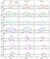 |
Fig. A.1. Line profiles of a 6.702 keV iron line for the different clusters at different distances from the cluster center (as written in each of the top panels). The intensity is in arbitrary units. For each panel, we also calculate the ratio between intensity for MFM and SPH to emphasize smaller differences. |
Appendix B: Surface density
In Fig. B.1 we show the surface density of all clusters. More active clusters such as g14 or g19 show a lot of substructure, while more relaxed clusters such as g63 show much less substructure. In g14 even two distinct cores in the center are visible as tracers of a recent major merger.
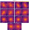 |
Fig. B.1. Projected gas density maps for all clusters analyzed in this work at redshift z = 0. The dashed circle denotes Rvir. |
All Tables
All Figures
|
Fig. 1. Projected gas density maps for g19 and g63 as examples of one more active and one more relaxed cluster analyzed in this work at redshift z = 0. The dashed circle denotes Rvir. The upper maps have a size of Δx = Δy ≈ 3064 kpc h−1; the lower maps Δx = Δy ≈ 2797 kpc h−1. |
| In the text | |
|
Fig. 2. Radial gas density, temperature, and entropy profiles for the clusters analyzed in this work at redshift z = 0. Lower panels show the ratio between MFM and SPH simulations for each cluster. |
| In the text | |
|
Fig. 3. Gas mass to halo mass relation for the clusters evaluated inside different radii at redshift z = 0. Lines indicate constant gas fractions, fgas. The colors of the clusters are the same as in Fig. 2. |
| In the text | |
|
Fig. 4. Evolution of the center offset and substructure-mass over time of all clusters analyzed in this work. As is described in Sect. 3.1, a cluster is classified as relaxed only if both lines are below the two dotted thresholds, and otherwise as active. The colors of the clusters are the same as in Fig. 2. |
| In the text | |
|
Fig. 5. Slice through the g55 cluster at redshift z = 0, showing the rotational component of the velocity in the upper panel and the multi-scale filtered velocity in the lower panel, each comparing MFM and SPH. The color indicates the absolute value of the solenoidal or filtered velocity, while the quivers show the direction. The dashed circle marks Rvir. |
| In the text | |
|
Fig. 6. Velocity profiles of all the simulated galaxy clusters, at redshift z = 0. The colors of the clusters are the same as in Fig. 2. The lower panels show the ratio between MFM and SPH simulations for each cluster. |
| In the text | |
|
Fig. 7. Turbulent pressure profile averaged over all clusters at redshifts z = 0.33 and z = 0, comparing the three analysis methods: the clump3d method, the solenoidal velocity component, and the multi-scale filtered velocity. The sample is split between dynamical states (left column: relaxed, right column: active) and hydro-methods (top row: MFM, bottom row: SPH) used for the simulation. The linestyle indicates the redshift, the color the analysis method. As only seven clusters were used for averaging, a strong scatter between individual clusters dominates the uncertainty. |
| In the text | |
|
Fig. 8. Turbulent pressure profile averaged over all clusters and redshifts 0.43 ≥ z ≥ 0. The sample was split between dynamical states and hydro-methods used for the simulation, shown in the different panels. The solid line shows the results for the Clump3d analysis, the dashed line the pressure resulting from the solenoidal velocity component using the Helmholtz-decomposed velocity, and the dash-dotted line results from the multi-scale filtering. The typical uncertainty is on the order of σ = 0.08 and indicated for each method with an error bar on the left of each panel. |
| In the text | |
|
Fig. A.1. Line profiles of a 6.702 keV iron line for the different clusters at different distances from the cluster center (as written in each of the top panels). The intensity is in arbitrary units. For each panel, we also calculate the ratio between intensity for MFM and SPH to emphasize smaller differences. |
| In the text | |
|
Fig. B.1. Projected gas density maps for all clusters analyzed in this work at redshift z = 0. The dashed circle denotes Rvir. |
| In the text | |
Current usage metrics show cumulative count of Article Views (full-text article views including HTML views, PDF and ePub downloads, according to the available data) and Abstracts Views on Vision4Press platform.
Data correspond to usage on the plateform after 2015. The current usage metrics is available 48-96 hours after online publication and is updated daily on week days.
Initial download of the metrics may take a while.