| Issue |
A&A
Volume 693, January 2025
|
|
|---|---|---|
| Article Number | A245 | |
| Number of page(s) | 14 | |
| Section | Numerical methods and codes | |
| DOI | https://doi.org/10.1051/0004-6361/202451348 | |
| Published online | 22 January 2025 | |
Search for hot subdwarf stars from SDSS images using a deep learning method: SwinBayesNet
1
School of Mathematics and Statistics, Shandong University,
Weihai,
264209
Shandong,
PR China
2
School of Mechanical, Electrical and Information Engineering, Shandong University,
Weihai,
264209
Shandong,
PR China
3
Key Laboratory of Stars and Interstellar Medium, Xiangtan University,
Xiangtan,
411105
Hunan,
PR China
★ Corresponding author; This email address is being protected from spambots. You need JavaScript enabled to view it.
Received:
2
July
2024
Accepted:
30
November
2024
Abstract
Hot subdwarfs are essential for understanding the structure and evolution of low-mass stars, binary systems, astroseismology, and atmospheric diffusion processes. In recent years, deep learning has driven significant progress in hot subdwarf searches. However, most approaches tend to focus on modelling with spectral data, which are inherently more costly and scarce compared to photometric data. To maximise the reliable candidates, we used Sloan Digital Sky Survey (SDSS) photometric images to construct a two-stage hot subdwarf search model called SwinBayesNet, which combines the Swin Transformer and Bayesian neural networks. This model not only provides classification results but also estimates uncertainty. As negative examples for the model, we selected five classes of stars prone to confusion with hot subdwarfs, including O-type stars, B-type stars, A-type stars, white dwarfs (WDs), and blue horizontal branch stars. On the test set, the two-stage model achieved F1 scores of 0.90 and 0.89 in the two-class and three-class classification stages, respectively. Subsequently, with the help of Gaia DR3, a large-scale candidate search was conducted in SDSS DR17. We found 6804 hot-subdwarf candidates, including 601 new discoveries. Based on this, we applied a model threshold of 0.95 and Bayesian uncertainty estimation for further screening, refining the candidates to 3413 high-confidence objects, which include 331 new discoveries.
Key words: methods: data analysis / methods: statistical / techniques: photometric / Hertzsprung-Russell and C-M diagrams / subdwarfs
© The Authors 2025
 Open Access article, published by EDP Sciences, under the terms of the Creative Commons Attribution License (https://creativecommons.org/licenses/by/4.0), which permits unrestricted use, distribution, and reproduction in any medium, provided the original work is properly cited.
This article is published in open access under the Subscribe to Open model. This email address is being protected from spambots. You need JavaScript enabled to view it. to support open access publication.
1 Introduction
Hot subdwarfs, which have a low mass of approximately half the solar mass (0.5 M⊙), display remarkably high effective temperatures (Teff) ranging from 20 000 to 70 000 K and surface gravities (log 𝑔) of between 5.0 and 6.5 dex (Lei et al. 2023a). Exhibiting spectral and colour similarities with O-type and B-type main sequence (MS) stars, hot subdwarfs are broadly classified into two categories based on their spectral line characteristics: sdO and sdB. The sdB stars, also known as extreme horizontal branch (EHB) stars, undergo helium (He) burning within their cores and are positioned towards the blue extremity of the horizontal branch (HB). The sdO stars have depleted their core helium, indicating that they are no longer in the He MS phase, and are evolving into white dwarfs (WD), and represent a blend of post-red giant branch (RGB), post-HB, and post-asymptotic giant branch (AGB) stars (Heber 2009, 2016). Furthermore, depending on the strength of the hydrogen (H) and He lines, hot subdwarfs can be subdivided into He-poor subdwarfs (sdB, sdOB, and sdO), which are dominated by the H lines, and He-rich subdwarfs (He-sdB, He-sdOB, and He-sdO), which are dominated by the He lines (Moehler et al. 1990; Geier et al. 2017; Lei et al. 2023b).
In the Hertzsprung-Russell (HR) diagram, hot subdwarfs are positioned between the MS and the WD sequence; while throughout the Milky Way galaxy, hot subdwarfs are widely distributed over all Galactic populations, including the thin disc, the thick disc, the bulge, and the halo (i.e. globular clusters) (Heber 2009).
Hot subdwarfs, characterised as low-mass celestial bodies, hold significant value for scientific research. Theoretically, it is unlikely for them to reach the helium-burning phase within the age of the Universe through normal stellar evolution. Therefore, the formation of hot subdwarfs is likely quite distinctive, and studying them can contribute to a better understanding of the evolutionary processes of low-mass stars. However, the formation mechanism of hot subdwarfs remains elusive. The several possible formation channels for hot subdwarfs include binary systems and single stars, with binary evolution being the main channel, involving Roche lobe overflow (RLOF), common envelope (CE) ejection, and a merger of two helium WDs (Han et al. 2002, 2003). As the majority of sdBs are discovered in close binaries (Napiwotzki et al. 2004; Copperwheat et al. 2011), hot subdwarfs can be used to study the evolution and formation of binary systems. Among them, hot subdwarf binaries with massive WD companions serve as candidates for the progenitors of type Ia supernovae (Wang et al. 2009; Wang & Han 2010; Geier et al. 2007, 2013, 2015a). Several types of pulsating stars found in hot subdwarfs can be used in astroseismology to study the internal structure and rotation of stars (Charpinet et al. 2011; Zong et al. 2018). The peculiar helium abundance of hot subdwarfs can be used to study diffusion processes; more details are available in Heber (2016).
Initially, hot subdwarfs were discovered in a survey of faint blue stars (Humason & Zwicky 1947). Subsequently, Kilkenny et al. (1988) and Østensen (2006) released catalogues containing 1225 and more than 2300 hot subdwarfs, respectively. With the publication of the Sloan Digital Sky Survey (SDSS), Large Sky Area Multi-Object Fiber Spectroscopic Telescope (LAMOST), and the addition of data from other large-scale surveys, significant progress has been made in the search for these objects. Geier et al. (2017) released the first relatively complete hot subdwarf catalogue containing 5613 hot subdwarfs. The release of Gaia DR2 (Gaia Collaboration 2018) is a milestone in the search for hot subdwarfs, as it provides colour, absolute magnitude, and reduced proper motion, which can be used as criteria for candidate selection. Based on this, Geier et al. (2019) released a catalogue of 39 800 candidates, and Geier (2020) released a second catalogue of 5874 known hot subdwarfs. Culpan et al. (2022) then continued Geier’s work by updating the known hot subdwarfs to 6616 and the candidates to 61 585 with the help of Gaia EDR3 (Gaia Collaboration 2021).
Conventional search methods for hot subdwarfs are based on the fundamental characteristics of these stars. Candidates are initially selected based on colour, and are then confirmed based on visual inspection and template matching of spectra (Geier et al. 2011, 2015b; Vennes et al. 2011; Németh et al. 2012; Kepler et al. 2015, 2016; Luo et al. 2016). However, as of 2018, Gaia Data Release 2 (DR2) provided parallax and photometric information that can be used to construct the HR diagram, facilitating a more efficient selection of candidates. Lei et al. (2018, 2019b, 2020, 2023a) and Luo et al. (2019, 2021) adopted this approach to select candidates in Gaia, which they then cross-matched with LAMOST, and further identified common sources through template matching. Initial screening of candidates through traditional methods is relatively crude, and the use of tabular data such as photometric magnitudes provides limited information, resulting in lower confidence in the candidates.
In recent years, machine learning and deep learning have been widely applied in various fields of astronomy, driving notable progress in the search for hot subdwarfs. Bu et al. (2017) first applied the hierarchical extreme learning machine (HELM) to find more than 7000 candidates in LAMOST DR1, 56 of which were identified as hot subdwarfs by Lei et al. (2019a). Subsequently, Bu et al. (2019) further improved the search efficiency based on convolutional neural networks (CNNs) and a support vector machine (CNN+SVM). Tan et al. (2022) found 2393 candidates in LAMOST DR7-V1 based on CNN, 25 of which were newly identified as hot subdwarfs. Most of the above focuses on modeling using spectral data. However, spectroscopic data are more expensive to obtain and are available in smaller quantities compared to photometric data. Therefore, in order to maximise the reliability of candidates, the present study focuses on searching for hot-subdwarf candidates based on the more abundant photometric data.
Given the above motivations, we used SDSS photometric images to construct a two-stage hot subdwarf search model based on SwinBayesNet. Subsequently, a large-scale candidate search in SDSS DR17 was conducted with the assistance of Gaia DR3. The organisational structure of this paper is as follows. Section 2 provides a detailed description of the data sources and sample distribution. Section 3 introduces the establishment of the classification model, SwinBayesNet, and the settings for the training strategy. In Sect. 4, we present our evaluation metrics and the results of the two-stage classification model, as well as the results of our comparative experiment. In Sect. 5, we describe how we applied the developed model to SDSS DR17 and we discuss the results obtained. Finally, in Sect. 6 we outline our conclusions.
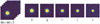 |
Fig. 1 Sample of photometric data. The left panel presents an example of the data used in this study, with dimensions of 48 × 48 × 5. Subsequently, examples of the u, ɡ, r, i, and ɀ bands from SDSS are displayed from left to right. |
2 Data
2.1 Data source
The SDSS is a large-scale survey project that uses a 2.5 meter telescope to collect multi-band photometric and spectral data for millions of objects. Since the year 2000, the survey has completed four phases. The imaging camera of SDSS began capturing images in 1998 and concluded in 2009. It scanned the sky in strips, with each strip containing six scan lines, each equipped with u, ɡ, r, i, and ɀ filters. Each imaging region corresponds to 2048 × 1489 pixels, and is uniquely determined by three parameters: run, camcol (camera column), and field. The complete image data were made public in the first data release (DR8, Hiroaki et al. 2011) of the third phase of SDSS (SDSS- III). Subsequent survey data releases no longer include new photometric images but involve multiple reprocessings of the photometric pipelines of the existing data. The data used in the present paper are derived from the final data release of the fourth phase of SDSS (SDSS-IV), specifically the photometric images from SDSS DR17 (Abdurro’uf et al. 2022).
With the assistance of CasJobs1, a data acquisition tool provided by SDSS, we obtained the three parameters (run, cam- col, and field) for each star from the photometric catalogue (PhotoObj) of SDSS DR17. Subsequently, we downloaded the original FITS files for the five bands (u, ɡ, r, i, and ɀ). After obtaining the original imaging regions (each 2048 × 1489 pixels), each star was cropped – with its right ascension (RA) and declination (Dec) as the centre – to a size of 48 × 48 pixels. Ultimately, each star is represented as a high-dimensional array of 48 × 48 × 5 (see Fig. 1). In this process, stars were filtered based on the clean flag, which is set to 1. The clean flag in SDSS is used to quickly select a clean sample of stars.
The positive sample of hot subdwarfs in this paper is derived from Culpan et al. (2022), resulting in a sample of 2958 stars after crossing with SDSS DR17. The negative sample comprises five classes of stars that are easily confused with hot subdwarfs, including O-type, B-type, and A-type stars, as well as WDs and blue horizontal branch stars (BHBs). Specifically, O-type, B-type, A-type, and WDs are all sourced from the SpecObj catalogue of SDSS DR17, while BHBs are obtained from Xue et al. (2008) and Vickers et al. (2021). Except for O-type stars, for each of the other star classes, 3000 stars were randomly selected. Due to the scarcity of O-type stars in SDSS DR17, only 1354 stars were chosen for this category. The total number of objects in the final sample is 16 312, and a summary of this sample is presented in Table 1.
2.2 Data distribution
Gaia, launched by the European Space Agency (ESA) in 2013, is a space astrometry satellite designed to accurately measure the positions, motions, luminosity, and colours of billions of stars, which are used to create a high-precision three-dimensional star map. Since the second data release (DR2), Gaia has provided photometric magnitudes in the blue (GBP) and red (GRP) bands, as well as the absolute magnitude in G band (MG), which can be used to construct the Gaia HR diagram. The HR diagram facilitates the search and study of various unique objects, particularly hot subdwarfs. The formula for calculating the MG is as follows:
 (1)
(1)
where G is the photometric magnitude in G band and ϖ is parallax.
Figure 2 presents the HR diagram of Gaia DR3. We note that the GBP − GRP of known hot subdwarfs (blue dots) concentrates around −0.35, while the MG is around 4.5. Of the 2958 hot subdwarfs in the sample of this study, 1931 have spectroscopic classifications in SDSS DR17. Among these, 1890 objects (approximately 98%) are classified by SDSS as O-type stars (395), B-type stars (872), and A-type stars (623). This result further confirms the rationale behind the selection of negative sample types in this paper.
Summary of sample.
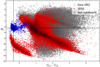 |
Fig. 2 HR diagram of Gaia DR3, where grey points represent samples from Gaia DR3, red points depict stars with spectral classifications in SDSS DR17, and blue points indicate samples of known hot subdwarfs. The two black dashed lines mark the concentrated distribution region of known hot subdwarfs (GBP − GRP ~ −0.35 and MG ~ 4.5). It is worth noting that the stars plotted on the figure have been filtered according to the criteria used for constructing the Gaia HR diagram, as detailed in Eq. (18). |
3 Method
3.1 Construction of classification model
Here, the search for hot subdwarfs is treated as a two-class classification, considering hot subdwarfs as positive samples and the remaining five classes (O, B, A, WD, BHB) as negative samples. However, using this approach, the F1 score (defined in Eq. (16)) for hot subdwarfs only reaches 0.8. Even though the ratio of positive to negative samples is close to 1:5, indicating an imbalance, various attempts to alleviate the imbalance did not significantly improve the F1 score. This suggests that sample imbalance is not the key factor leading to the lower F1 score. By examining misclassified objects, it was observed that they were predominantly O-type stars and WDs. Hence, the primary reason for the lower F1 score lies in the similarity between these two classes of stars and hot subdwarfs. It is necessary to further refine these three classes by developing a more focused feature-extraction model.
We therefore propose a two-stage classification model. The positive and negative sample settings of the model, along with the sample sizes, are shown in Table 2. In the first stage, hot subdwarfs, O-type stars, and WDs are treated as one class, and a two-class classification model is employed to filter out B-type stars, A-type stars, and BHBs. In the second stage, a three-class classification is performed on the samples classified as positive in the first stage, including hot subdwarfs, O-type stars, and WDs. The dataset is divided into training, validation, and testing sets in a ratio of 6:2:2.
However, the two-stage classification model alone is insufficient to address all of the challenges faced when using this kind of approach. We observe that the model’s confidence levels for O-type stars and WDs are unstable, leading to frequent misclassifications. Due to the high similarity between these stars and hot subdwarfs, the model often exhibits overconfidence, outputting high predicted probabilities for uncertain objects. This phenomenon aligns with common issues in neural networks, especially deep neural networks. The model uses the softmax function to produce predicted probabilities for each class, reflecting its relative judgments based on the current parameters and input data. While a higher value indicates a stronger inclination towards a specific class, it may not accurately represent the true probability that a target belongs to that class.
To address this problem, we introduce a Bayesian framework to quantify the predictive confidence of the model through uncertainty estimation. Specifically, we combine the Swin Transformer with Bayesian neural networks (BNNs) to construct the SwinBayesNet model. This model not only outputs classification results but also estimates uncertainty, allowing us to exclude samples with high predicted probabilities that also exhibit high uncertainty, thus providing more scientifically high-confidence candidates. In the following sections, we detail the design and implementation of the Swin Transformer, BNNs, and the Swin- BayesNet model.
Sample settings and sizes of the two-stage model.
3.2 Swin Transformer
The Swin Transformer model (Liu et al. 2021) is a hierarchical vision Transformer model based on shifted windows and designed specifically for advanced image-analysis tasks. It was awarded the ‘Best Paper’ at the International Conference on Computer Vision (ICCV) in 2021 and has since become widely used in the computer vision field. It has proven particularly effective at tasks such as image classification, object detection, and semantic segmentation.
In the field of computer vision, convolutional neural networks (CNNs) have become the leading architecture. These networks extract features from images layer by layer using convolutional layers and then reduce data dimensions by pooling layers. Ultimately, they produce classification results through fully connected layers. Meanwhile, in the field of natural language processing, the Transformer architecture (Vaswani et al. 2017) has gained prominence due to its attention mechanism, which effectively handles long sequences of data. In 2020, the Vision Transformer (ViT, Dosovitskiy et al. 2021) was introduced, marking the first direct application of the Transformer model from natural language processing to computer vision. Building on this foundation, the Swin Transformer was developed as an enhanced Transformer version specifically designed for computer vision tasks. It extracts features layer by layer like CNNs, while overcoming the limitations of the single-resolution feature maps used in ViT.
Specifically, the Swin Transformer introduces two optimisations. Firstly, it introduces a patch merging layer (see Sect. 3.2.1) to construct a hierarchical feature map. This layer halves the height and width of the feature map while doubling the number of channels. This makes it particularly effective for tasks like semantic segmentation and object detection, which require precise identification and localisation of small objects within images. Secondly, to reduce computational complexity, it avoids calculating self-attention across the entire feature map. Instead, it divides the feature map into smaller, non-overlapping windows and computes self-attention within each window. Interaction between windows is achieved through an operation called shifted windows (see Sect. 3.2.2).
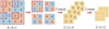 |
Fig. 3 Structure of the patch merging operation. A 4 × 4 × 1 feature map is transformed into a 2 × 2 × 2 map. The 4 × 4 feature map is divided into 2 × 2 blocks, totaling 4 blocks. The four elements of each block are labelled 1–4. |
3.2.1 Patch merging
Patch merging is a downsampling operation similar to the pooling operation of CNNs, but unlike pooling, patch merging does not lose information. As illustrated in Fig. 3, we consider a single-channel feature map with a size of 4 × 4. When the downsampling factor is 2, the map is divided into 2 × 2 blocks. For each block (consisting of four elements), the elements at the corresponding positions are combined to form four feature maps, each with a size of 2 × 2. Subsequently, these feature maps are concatenated along the channel dimension. Finally, a linear layer is applied to map the four feature maps into two feature maps. Through this operation, the height and width of the feature map are halved, while the number of channels is doubled (from 4 × 4 × 1 to 2 × 2 × 2).
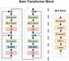 |
Fig. 4 Swin Transformer block. This block is composed of two stacked Transformer encoders, W-MSA and SW-MSA. The rightmost panel illustrates the structure of the MLP block within the Swin Transformer block. |
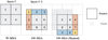 |
Fig. 5 Attention calculation process in the Swin Transformer block. The left panel represents the use of W-MSA in the layer l, the middle panel represents the use of SW-MSA in the next layer, and these two appear in pairs. The attention calculation in SW-MSA is shown in the right panel, where the completion of the new window is achieved by moving the windows and then a masking operation is applied to calculate attention within the window. Please note that the black squares represent windows with a size of 4 × 4, and the grey squares represent patches. |
3.2.2 Swin Transformer block
The Swin Transformer block (see Fig. 4) is a fundamental component of the Swin Transformer architecture. It consists of two types of Transformer encoders: window-based multi-head self-attention (W-MSA) and shifted window-based multi-head self-attention (SW-MSA). Unlike the self-attention mechanism used in ViT, which considers the entire feature map, W-MSA computes self-attention within smaller, non-overlapping windows of the feature map. This approach conserves computational resources, making it more efficient. However, a limitation is that the windows do not interact with one another, limiting the model’s ability to capture all of the information contained within the data. To address this limitation, SW-MSA is introduced, allowing for information sharing among different windows and thereby improving interaction.
As illustrated in Fig. 5, assume the feature map is singlechannel with a size of 8 × 8. The Swin Transformer divides this feature map into non-overlapping windows, each with a size of 4 × 4 (M = 4). In layer l, the feature map is divided into  windows, and self-attention is computed within these 4 windows. Subsequently, in layer l + 1, the entire feature map is shifted to the right and down by 2 pixels
 ![Mathematical equation: $\left( {\left[ {{M \over 2}} \right]} \right)$](/articles/aa/full_html/2025/01/aa51348-24/aa51348-24-eq3.png) , leading to a new division of windows. At this point, the feature map is divided into 9 windows. Calculating attention within these 9 windows enables interaction between the windows from layer l. For instance, when computing attention within window 2 at layer l + 1, interaction information between window 1 and window 2 from layer l can be obtained. However, these 9 windows have different sizes. To perform parallel attention computation across these 9 windows, we need to pad them to a uniform size of 4 × 4, which increases the computational complexity compared to the 4 windows in layer l.
, leading to a new division of windows. At this point, the feature map is divided into 9 windows. Calculating attention within these 9 windows enables interaction between the windows from layer l. For instance, when computing attention within window 2 at layer l + 1, interaction information between window 1 and window 2 from layer l can be obtained. However, these 9 windows have different sizes. To perform parallel attention computation across these 9 windows, we need to pad them to a uniform size of 4 × 4, which increases the computational complexity compared to the 4 windows in layer l.
To address this issue, we introduced a masked MSA mechanism. Specifically, window 1 from layer l + 1 (yellow region in the diagram) is moved to the bottom-right corner of window 9. The combination of windows 2 and 3 (blue region) is shifted to the bottom of windows 8 and 9, and the combination of windows 4 and 7 (orange region) is moved to the right of windows 6 and 9. This rearrangement forms 4 new windows, and attention needs to be computed within these new windows. However, as some of these new windows, for example window 4 and window 6, are not continuous in practice, attention must be computed separately for each window. For instance, when calculating attention for window 4, the weights related to window 6 are set to zero, ensuring that only the internal attention within window 4 is considered. Similarly, when calculating attention for window 6, the weights related to window 4 are set to zero.
The attention calculation formula is as follows:
 (2)
(2)
where Q, K, and V represent the query, key, and value, respectively, d is the dimension of query or key, and B denotes the relative position bias used in the Swin Transformer.
3.3 Bayesian neural networks
No neural network can be universally applied to all data distributions. Complex neural networks are prone to overfitting due to their large number of parameters, which affects the model’s generalisation ability. Additionally, standard neural networks often exhibit overconfidence. Even when the model’s predicted result is incorrect, it may still give a high predicted probability, indicating that the model is overly confident in its predictions and unable to measure the uncertainty of its results. To address these issues, BNNs (Blundell et al. 2015) were introduced.
Standard neural networks treat the model’s weight parameters as fixed constants. Once training is complete, these parameters are set, resulting in consistent results for a given input. However, a single deterministic output cannot capture the uncertainty in predictions. In contrast, BNNs treat the model’s parameters as probability distributions, classifying them as stochastic neural networks. During multiple forward propagations, the same input can produce different results, allowing us to quantify prediction uncertainty.
Bayesian neural networks are based on Bayes’s theorem, which can be expressed in the context of neural networks as follows. With the dataset denoted Ɗ(X, y) and the model’s weight parameters as θ, Bayes’s theorem is formulated as
 (3)
(3)
where p(θ) represents the prior probability, reflecting our initial assumptions about the model parameters; p(Ɗ) is the marginal probability (also known as evidence), indicating the probability distribution of observing the dataset; p(Ɗ | θ) is the likelihood function, which describes the data generation process, indicating the probability of generating the dataset Ɗ given the model parameters θ; and finally p(θ | Ɗ) is the posterior probability, representing the updated probability distribution of the model parameters θ after observing the dataset Ɗ.
Bayes’s theorem can be understood as follows. Initially, we have a preliminary understanding of the probability distribution of the parameters θ based on our prior assumptions. As we observe the dataset Ɗ, we update our understanding of these parameters, leading to the posterior distribution. Within this Bayesian framework, BNNs not only provide classification results but also quantify the uncertainty of the predictions.
As the dataset Ɗ represents a conditional probability distribution p(y | X), and X is independent of θ, we can deduce that p(θ) = p(θ | X). Based on this, the posterior probability can be further expressed as
 (4)
(4)
If we can compute this posterior probability, we can obtain the probability distribution of the parameters. However, as seen in the equation, the denominator p(y | X) requires integration over all possible values of θ, and the exact solution is often computationally unfeasible.
Therefore, in practical applications, approximate inference methods are commonly used, including Markov chain Monte Carlo (MCMC) methods and variational inference. Due to the high computational costs and extensive iterations required by MCMC, BNNs typically favour variational inference. The fundamental principle of variational inference is to find a variational distribution qϕ(θ) that closely approximates the posterior distribution p(θ|X,y), using Kullback-Leibler (KL) divergence to measure the difference between the two distributions. The KL divergence is then minimised to optimise the variational distribution.
A widely used method for variational inference in BNNs is Bayes by Backprop, which was introduced by Blundell et al. (2015). This method is designed to minimise the following KL divergence:
 (5)
(5)
After some derivation, we obtain
 (6)
(6)
Since the last term, log p(y|X), is independent of ϕ, we get
![Mathematical equation: $\eqalign{ & {\phi ^*} = \arg \mathop {\min }\limits_\phi {\mathop{\rm KL}\nolimits} \left( {{q_\phi }(\theta )p(\theta \mid X,y)} \right) \cr & \,\,\,\,\,\, = \arg \mathop {\min }\limits_\phi \left( {{\mathop{\rm KL}\nolimits} \left( {{q_\phi }(\theta )p(\theta )} \right) - {_{{q_\phi }}}[\log (p(y\mid X,\theta )]).} \right. \cr} $](/articles/aa/full_html/2025/01/aa51348-24/aa51348-24-eq9.png) (7)
(7)
For clarity, let
![Mathematical equation: $\eqalign{ & {\cal F}(y,X,\phi ) = {\mathop{\rm KL}\nolimits} \left( {{q_\phi }(\theta )p(\theta )} \right) - {_{{q_\phi }}}[\log (p(y\mid X,\theta ))] \cr & \,\,\,\,\,\,\,\,\,\,\,\,\,\,\,\,\,\,\,\,\,\,\,\, = \int {{q_\phi }} (\theta )\log {{{q_\phi }(\theta )} \over {p(\theta )p(y\mid X,\theta )}}{\rm{d}}\theta \cr & \,\,\,\,\,\,\,\,\,\,\,\,\,\,\,\,\,\,\,\,\,\,\,\, = \int {{q_\phi }} (\theta )\left[ {\log {q_\phi }(\theta ) - \log p(\theta ) - \log p(y\mid X,\theta )} \right]{\rm{d}}\theta , \cr} $](/articles/aa/full_html/2025/01/aa51348-24/aa51348-24-eq10.png) (8)
(8)
where ℱ (y, X, ϕ) is referred to as the variational free energy. The optimisation goal can be rewritten as minimising the variational free energy:
 (9)
(9)
Finally, as the integrals in the above formula are difficult to compute directly, Monte Carlo methods are often used to estimate the variational free energy. The equation can be discretised as
![Mathematical equation: ${\cal F}(y,X,\phi ) \approx {1 \over m}\sum\limits_{i = 1}^m {\left[ {\log {q_\phi }\left( {{\theta ^i}} \right) - \log p\left( {{\theta ^i}} \right) - \log p\left( {y\mid X,{\theta ^i}} \right)} \right]} .$](/articles/aa/full_html/2025/01/aa51348-24/aa51348-24-eq12.png) (10)
(10)
However, the sampling process is non-differentiable, which means it cannot be directly optimised using gradient descent. To address this issue, the reparameterisation trick is typically employed, which involves first sampling from a non-parametric distribution and then transforming it to ensure differentiability. In Bayes by Backprop, this method entails sampling each weight individually and combining them with the inputs. In the present paper, we adopt a local reparameterisation trick inspired by Bayes by Backprop (Kingma et al. 2015). This method allows direct sampling from the activation distribution, thereby reducing computational costs and improving efficiency.
 |
Fig. 6 Overall model framework, divided into three main parts. The input part is a high-dimensional matrix with dimensions of 48 × 48 × 5. The feature extraction consists of five stages, with the Swin Transformer block (in blue) detailed in Sect. 3.2.2, and the patch merging (in green) described in Sect. 3.2.1. Numbers within the Swin Transformer blocks denote the repetition of stacked blocks. The third part is the head for the classification output, where the Bayesian block (see Fig. 7) maps the 8C-dimensional features to 2 or 3, corresponding to two-class and three-class classification, while also outputting the uncertainty. |
3.4 SwinBayesNet
As mentioned in Sect. 3.1, we constructed the SwinBayesNet model by combining the Swin Transformer and BNNs. The model is initially trained for two-class and three-class classification using the Swin Transformer. Once the model is trained stably, we freeze the backbone (feature extraction) and replace the output head with a BNN to produce the final classification results and uncertainty.
The model’s overall framework is illustrated in Fig. 6, where photometric images of stars are input to the network as a highdimensional matrix of size 48 × 48 × 5. Subsequently, feature extraction is conducted through five stages. At stage 0, the PatchEmbed module is employed to break down the photometric image into patches, each of 2 × 2 in size, mapping the channel dimension to C and thus transforming the dimensions to 24 × 24 × C. For the two-class and three-class classification models, C is set to 128 and 192, respectively. Each stage from stage 1 to 3 consists of Swin Transformer blocks and a patchmerging module, while stage 4 only contains Swin Transformer blocks. The Swin Transformer blocks compute attention, while patch merging adopts a CNN-like approach for downsampling. Through three downsampling operations, the feature map of the original photometric image is reduced from 48 × 48 to 3 × 3, with the number of channels changing from 5 to 8C. It then undergoes a layer normalisation (LN) layer and a global average pooling layer, transforming the feature map from 3 × 3 × 8C to a feature vector of size 8C. After feature extraction, we freeze the backbone and input the extracted features into the Bayesian block (see Fig. 7) for further training of the BNN, which outputs both classification results and uncertainty.
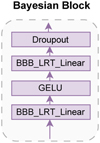 |
Fig. 7 Bayesian block composed of BBB_LRT_Linear layers (using the local reparameterisation trick) and GELU activation and dropout layers. |
3.5 Training strategy
As the data are essentially high-dimensional arrays, unlike traditional computer vision image data, many data-augmentation methods related to brightness and colour changes cannot be applied here. Therefore, we only employed random flips and rotations. Specifically, we applied horizontal and vertical flips with a probability of 0.3, and applied random rotations within a range of 90 degrees.
In the Swin Transformer classification model, the loss function is the cross-entropy loss function, and is expressed as
 (11)
(11)
where n is the number of samples, m denotes the number of categories, yic represents the label of sample yi, indicating whether yi belongs to category c, and ŷic indicates the probability that the sample yi is predicted to belong to category c. For the two-class classification model, the weights are initialised using truncated normal distribution, and the base learning rate is set to 1 × 10⁻⁴. For the three-class classification model, Xavier initialisation is used, and the base learning rate is set to 3 × 10⁻⁵. Both models are trained for 100 epochs with a batch size of 128 using the Adam optimiser. The weight decay is configured at 1 × 10⁻⁵ for both models.
In the Bayesian block, the loss function is given by Eq. (8), which consists of two parts: the KL divergence (prior-dependent part) and the negative log-likelihood (data-dependent part). The negative log-likelihood can be computed using the negative loglikelihood loss (NLLLoss), which is expressed as
 (12)
(12)
where ŷi is the predicted probability for the true label of the i-th sample. Both models are trained for 500 epochs with a batch size of 256.
Confusion matrix.
4 Result
4.1 Evaluation metrics
The model evaluation metrics include the confusion matrix (see Table 3), as well as the accuracy, precision, recall, and F1 score (defined below), which are commonly used for classification tasks. Accuracy is the proportion of correctly predicted objects to the total number of objects. Precision indicates the proportion of objects predicted to be hot subdwarfs by the model that are actually hot subdwarfs, while recall indicates the proportion of hot subdwarf objects that the model can correctly predict. F1 score is the harmonic mean of precision and recall, serving as a comprehensive evaluation metric. Given that this study focuses on the search for hot subdwarfs, it is more interested in the metrics related to this class of stars, namely precision, recall, and F1 score for hot subdwarfs.
 (13)
(13)
 (14)
(14)
 (15)
(15)
 (16)
(16)
Performance of the two-class classification model.
4.2 Results of the two-class classification model
For the two-class classification model, positive samples comprise a mixture of hot subdwarfs, O-type stars, and WDs, while negative samples consist of a mixture of B-type, A-type, and BHB stars.
After 100 epochs, the Swin Transformer two-class classification model stabilises (see Fig. 8b). Subsequently, we froze the backbone and trained the Bayesian block. After 500 epochs, the model also stabilised (see Fig. 8c) and produced results on the test set, achieving an overall accuracy of 0.92. For positive samples, the precision is 0.94, recall is 0.87, and the F1 score is 0.90. The performance and confusion matrix of the two- class classification model are detailed in Table 4 and Fig. 9, respectively.
4.3 Results of the three-class classification model
After 100 epochs of iteration, the Swin Transformer three-class classification model stabilises (see Fig. 8e). We then froze the backbone and trained the Bayesian block. Finally, the model stabilised (see Fig. 8f) and produced results on the test set, achieving an overall accuracy of 0.82. For hot subdwarfs, the precision is 0.86, recall is 0.92, and the F1 score is 0.89. The performance and confusion matrix of the three-class classification model are detailed in Table 5 and Fig. 10, respectively. Compared to the two-class classification model, both the accuracy and the F1 score for hot subdwarfs have decreased, and especially the accuracy. This is primarily due to the involvement of classifying hot stars and white dwarfs.
Firstly, O-type stars present significant challenges. Their precision and recall are 0.68 and 0.56, respectively, resulting in a low F1 score of 0.61. This is partly because O-type stars are rare in SDSS DR17, numbering less than 2000, and their high temperatures make the labels provided by SDSS less reliable. This poor performance is consistent with previous research on the use of SDSS photometric images for stellar classification (see Shi et al. 2023).
Secondly, for WDs, the precision and recall are 0.83 and 0.85, respectively, with an F1 score of 0.84. These results are better than those for O-type stars, but are not ideal. This is mainly due to the similarity between hot subdwarfs and WDs in photometry and spectra, and the resulting difficulty in distinguishing between them, as demonstrated by Tan et al. (2022).
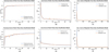 |
Fig. 8 Learning curves of the models. The first row presents the two-class classification model, with (a) and (b) representing the accuracy and loss curves for the Swin Transformer two-class model, respectively, while (c) shows the loss curve of the Bayesian two-class model. The second row displays the three-class classification model, where (d) and (e) represent the accuracy and loss curves for the Swin Transformer three-class model, and (f) shows the loss curve of the Bayesian three-class model. |
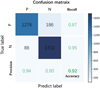 |
Fig. 9 Confusion matrix of the two-class classification model. |
Performance of the three-class classification model.
4.4 Comparative experiment
To demonstrate the efficiency of the model in searching for hot subdwarfs, a series of comparative experiments were conducted in this study.
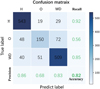 |
Fig. 10 Confusion matrix of the three-class classification model. |
4.4.1 Comparison of different data types
The photometric magnitudes in SDSS are obtained by processing the original photometric images and calculating them through mathematical models. These magnitudes provide a comprehensive summary of the information contained in the photometric images. Among them, PSF magnitudes are determined by fitting the point spread function (PSF) of objects, making them particularly suitable for describing point sources, such as isolated stars. Each band’s photometric magnitude in SDSS is represented by a numerical value, and so each star is represented as a vector with a length of 5 (psf Ma𝑔_u, psf Ma𝑔_𝑔, psf Ma𝑔_r, psf Ma𝑔_i, psf Ma𝑔_z).
To illustrate the advantage of using photometric images over photometric magnitudes in the search for hot subdwarfs, we acquired PSF magnitudes for 16 312 samples. We then applied machine learning algorithms, including support vector machine (SVM; Cortes & Vapnik 1995), random forest (RF; Breiman 2001), XGBoost (Chen & Guestrin 2016), LightGBM (Ke et al. 2017), and CatBoost (Prokhorenkova et al. 2018). We compared their performances with that of our model based on photometric images. The detailed results are presented in Table 6.
The table reveals that the proposed model based on photometric images performs the best, both in two-class and three-class classification. In the two-class classification model, the machine learning model based on photometric magnitudes shows similar performance to our proposed model. However, in the three-class classification model, our model performance has a clear advantage. This indicates that when dealing with the three easily confused classes, namely O-type stars, WDs, and hot subdwarfs, photometric images can provide more highdimensional and abstract features compared to photometric magnitudes. Therefore, they are better suited to the search for hot subdwarfs.
Our comparison of model performance led us to the conclusions outlined above. We now further explore the superiority of photometric images. Firstly, from the perspective of featureextraction methods, PSF magnitudes extract photometric information by fitting a PSF based on two-dimensional Gaussian and Moffat distributions (see Eq. (17)). This method solidifies the feature-extraction process, resulting in a generic photometric representation. Consequently, when using such data for classification tasks, models can only be further trained on this generic feature basis. In contrast, deep learning models based on original photometric images can automatically learn features tailored to specific classification tasks. During training, these models compute losses based on classification results and optimise feature extraction through gradient backpropagation, achieving adaptive adjustments for specific tasks and thus improving classification accuracy.
 (17)
(17)
Secondly, from the perspective of data dimensionality, photometric magnitudes are one-dimensional tabular data, whereas photometric images are two-dimensional data and serve as the source of magnitudes, inherently containing more information. Utilising this more original and information-rich data source enhances classification performance
Finally, the research by Wu et al. (2023) demonstrates that it is feasible to directly estimate Teff and log ɡ from photometric images, particularly in cases where log ɡ >4. These parameters are key characteristics of hot subdwarfs, and the study shows that its estimation method outperforms magnitude-based methods, further indicating that photometric images provide more crucial information, which aligns with our conclusions.
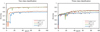 |
Fig. 11 Accuracy on the validation set varies across epochs for different numbers and combinations of bands. |
Performance comparison of using photometric magnitudes and images.
4.4.2 Comparison of different bands
The SDSS photometric image consists of five different bands. To investigate the impact of using different numbers and combinations of bands on the final classification performance, we conducted four comparative experiments: using all five bands (u, ɡ, r, i, ɀ), using two different combinations of four bands (u, ɡ, r, i and ɡ, r, i, ɀ), and using three bands (ɡ, r, i). Figure 11 shows the relationship between the accuracy and the epoch of these four experiments. The accuracy of five-band and four-band (u, ɡ, r, i) configurations is the highest, with a slight difference between them. In contrast, the accuracy of the four-band (ɡ, r, i, ɀ) and three-band (ɡ, r, i) configurations is lower. Considering the performance on the test set and aiming to use as much data as possible, we ultimately chose the five-band photometric image for classification.
4.4.3 Comparison of different deep learning models
To illustrate the superiority of our model in the search for hot subdwarfs, we compared its performance with that of typical and advanced deep learning models, including CNN-based methods such as VGG-16 (Simonyan & Zisserman 2015), ResNet-50 (He et al. 2016), EfficientNetV2-S (Tan & Le 2021), and ConvNext- B (Liu et al. 2022), as well as ViT. The results are shown in Table 7, highlighting that our approach outperforms others in both two-class and three-class classification.
This advantage arises from the Swin Transformer’s exceptional feature-extraction capabilities, which effectively capture both local and global features. While CNNs excel in extracting local features, they often struggle with integrating global information. ViT applies the Transformer architecture from natural language processing directly to computer vision without tailored optimisations for visual tasks, resulting in insufficient local feature extraction and a lack of multi-scale feature representation. In contrast, the Swin Transformer uses a hierarchical structure and a window-based self-attention mechanism, enabling it to process local features while simultaneously capturing global contextual information. This dual approach allows a more comprehensive understanding of image structures and relationships, significantly enhancing the modelling of spatial relationships and local features.
Performance comparison of different deep learning models.
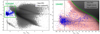 |
Fig. 12 Target selection for our hot subdwarfs search. The left panel shows the preliminary selection in Gaia DR3 (green rectangle), with blue and grey dots representing hot subdwarfs and objects from Gaia DR3, respectively. The right panel is an enlarged view of the left panel’s selection, revealing further refinement of the search region (green curve), with the region below the curve indicating the target sources (pink dots) for the hot subdwarfs search. |
5 Application
5.1 Target selection
After establishing the model, we applied it to actual survey data to validate its capacity in finding hot subdwarfs in real data. Our model is based on SDSS photometric images, the ideal approach would involve an extensive search across all photometric images from SDSS DR17. However, given the colossal scale of the photometric data in SDSS DR17, which contains information for approximately 1.2 billion objects, and considering the known properties and distribution of hot subdwarfs, we integrated distance information from Gaia DR3 and performed an initial region selection in the HR diagram (see the region below the green curve in the right panel of Fig. 12). Subsequently, we conducted a cross-match between SDSS DR17 and Gaia DR3, focusing on common sources for the search of hot subdwarfs.
Based on this, the target sources for searching hot subdwarfs in this study come from two sets of data. The first set is derived from 61 585 hot subdwarf candidates provided by Culpan et al. (2022), which have undergone astronomical filtering. After cross-matching with SDSS DR17 and applying a clean filter, we obtained 10 416 candidates. The purpose of utilising this dataset is to obtain candidates with higher confidence values.
The second set is obtained using the following Eqs. (18) and (19).
 (18)
(18)
 (19)
(19)
Equation (18) defines the criteria for constructing the Gaia HR diagram. In this equation, RPlx denotes the ratio of parallax to its standard error, while RFBP and RFRP represent the integrated mean flux divided by its error in the BP and RP bands, respectively.
Equation (19) is derived based on the distribution of known hot subdwarfs. Initially, as shown in the left panel of Fig. 12, a rectangular region is outlined in the HR diagram based on the distribution of hot subdwarfs (−1 < MG < 7 and −0.7 < BP – RP < 0.7). This region contains a total of 3182334 stars. The right panel is an enlarged view of the rectangular region in the left panel, with a curve (the third expression of Eq. (19)) drawn to exclude most MS stars. This curve is similar to Culpan’s, but it encompasses a larger range, and is designed to include as many target regions as possible for a more comprehensive search for hot subdwarfs. Below the curve of the rectangular region, there is a total of 194 482 stars. After cross-matching with SDSS DR17 and applying a clean filter, 29 034 stars were obtained.
The two sets of data were mutually de-duplicated, resulting in a final set of 37 519 stars as target sources for searching for hot subdwarfs.
Result comparison of other known hot subdwarf catalogues.
5.2 Search for hot subdwarfs
The above-mentioned target sources were input into the pretrained two-stage classification model, which recognised a total of 10 579 stars as positive samples. Subsequently, these stars were fed into the three-class classification model. A total of 6804 stars were recognised as hot subdwarfs by this latter model, including 601 stars not previously discovered by Culpan.
To validate the effectiveness of our research method, we compared our results with three known hot subdwarf catalogues, namely those of Geier et al. (2017), Geier (2020), and Culpan et al. (2022). All three catalogues employed the same data processing method as this study, specifically cross-matching with SDSS DR17 and applying clean filtering. As shown in Table 8, our target sources selected in Sect. 5.1 covered 83, 85, and 86% of the objects from these catalogues, with overall search accuracies for hot subdwarfs using our method of 77, 80, and 81%. Notably, the search accuracy within the coverage range reached 93, 94, and 94%. Therefore, as long as the hot subdwarfs are covered by the target sources, the probability of detection remains very high. These results indicate that our target selection is reasonable and our search method is effective. Among the 1352 uncovered objects, 1345 have common sources with Gaia DR3, of which 1329 (approximately 92%) do not meet the criteria for plotting the HR diagram (Eq. (18)) and are therefore excluded.
5.3 Uncertainty analysis
In BNNs, for classification tasks, Varq ( p(y* | x∗)) represents the variance of the conditional probability distribution of the target variable y* given the input x*, reflecting the variance due to model uncertainty.
Therefore, the measurement of uncertainty can be decomposed as follows (Kendall & Gal 2017):
![Mathematical equation: $\eqalign{ & {{\mathop{\rm Var}\nolimits} _q}\left( {p\left( {{y^*}\mid {x^*}} \right)} \right) = {_q}\left[ {y{y^T}} \right] - {_q}[y]{_q}{[y]^T} \cr & \,\,\,\,\,\,\,\,\,\,\,\,\,\,\,\,\,\,\,\,\,\,\,\,\,\,\,\,\,\,\,\,\,\,\,\,\,\, = \underbrace {{1 \over T}\sum\limits_{t = 1}^T {{\mathop{\rm diag}\nolimits} } \left( {{{\hat p}_t}} \right) - {{\hat p}_t}\hat p_t^T}_{{\rm{aleatoric }}} + \underbrace {{1 \over T}\sum\limits_{t = 1}^T {\left( {{{\hat p}_t} - \bar p} \right)} {{\left( {{{\hat p}_t} - \bar p} \right)}^T}}_{{\rm{epistemic }}}, \cr} $](/articles/aa/full_html/2025/01/aa51348-24/aa51348-24-eq22.png) (20)
(20)
where T is the number of forward passes, which is set to 50 in this paper.  denotes the predicted probability at the t-th forward pass, while
  is the mean predicted probability, defined as
  , representing the average probability across all T predictions.
Aleatoric uncertainty (also known as statistical uncertainty) arises from inherent noise in the data and cannot be reduced by adding more samples. In contrast, epistemic uncertainty is associated with the model itself, meaning that additional samples can improve its performance. For both types of uncertainty, we employed the Softmax method (Kwon et al. 2020) and the Softplus normalisation method (Shridhar et al. 2018), which are both based on model outputs, allowing us to derive four types of uncertainty, as follows:
 (21)
(21)
 (22)
(22)
In this study, we combined the four types of uncertainty derived from the model outputs and their predicted probabilities to identify high-confidence candidates. Specifically, we plotted the density distributions of these uncertainties (see Fig. 13) and selected objects that fell within the 95th percentile and had predicted probabilities of greater than 0.95 in the two-stage model, labelling them as high-confidence candidates. Ultimately, among the 6804 hot subdwarf candidates identified in Sect. 5.2, 3413 objects were classified as high-confidence candidates. Of the newly discovered 601 candidates, 331 were deemed high- confidence. A partial example of the hot subdwarf candidates catalogue is shown in Table 9 (the complete version includes 6804 candidates).
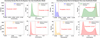 |
Fig. 13 Uncertainty density plots for the Bayesian two-class and three-class classification models. |
Catalogue of hot subdwarf candidates.
5.4 Related discussion
Figure 14 shows the sample distribution of hot subdwarf candidates obtained in this study (yellow and red points). The left panel displays the distribution of these objects in the Gaia DR3 HR diagram. It can be observed that the candidates are predominantly distributed in the region where hot subdwarfs are distributed (blue points). However, some candidates extend to the right of the HR diagram, connecting with the MS, resulting in a more widespread distribution. We can also see that some newly discovered candidates (red dots) are distributed near the green boundary line, especially in the lower-right region of the HR diagram.
Apart from the misclassifications induced by the model itself, this phenomenon may be attributed to two other factors. Firstly, binary systems with a WD and a low-mass MS companion exhibit a redder composite colour. This causes the hot subdwarfs in these binary systems to shift towards the redder end of HR diagram, approaching the MS region. Secondly, the influence of interstellar extinction leads to a darkening and reddening of celestial bodies, causing them to move towards the lower-right corner of the HR diagram. Consequently, actual hot subdwarfs deviate from their typical distribution region in the observation of photometric data, making them prone to being overlooked during the selection of candidates.
For these reasons, the target selection (see Sect. 5.1) in the present paper covers a wider range compared to Culpan’s and previous research, with the aim being to retain as many potential hot subdwarf targets as possible. Thus, the newly discovered candidates in this study that are situated near the boundary line are likely to be either hot subdwarfs in binary systems or objects overlooked due to their displacement to the lower-right of the HR diagram due to extinction.
The right panel of Fig. 14 shows the sky distribution of candidates obtained in this study, displaying their RA and Dec. Since SDSS photometric data mainly cover the northern celestial hemisphere, candidates obtained from SDSS photometric images are primarily distributed in the northern sky.
As shown in Fig. 15, currently known hot subdwarfs are widely distributed across the entire sky (green dots in the left panel). The target sources selected through Gaia in Sect. 5.1 also span the entire sky (grey dots in the left panel). Conducting a search for hot subdwarfs within this range will lead to a more comprehensive study. However, due to the limited coverage of SDSS photometric data, the search range in this study (grey dots in the right panel) is predominantly concentrated in the northern celestial hemisphere. Future plans include the use of the Pan-STARRS survey for the entire sky and the SkyMapper survey in the southern sky to conduct a more comprehensive study. This will focus on regions observable by Gaia but not covered by SDSS, including parts of the northern sky and the entire southern sky.
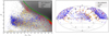 |
Fig. 14 Sample distribution of hot subdwarf candidates in this study. The left panel shows the distribution of samples predicted as hot subdwarfs by the model in the Gaia DR3 HR diagram. Blue points represent known hot subdwarfs, yellow points represent candidates discovered in this study that have already been reported by Culpan, and red points represent newly discovered candidates in this study. Each plotted sample has passed the screening criteria defined in Eq. (18). The right panel displays the sky distribution of all samples. |
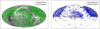 |
Fig. 15 Sky distribution of target sources and hot subdwarfs. The left panel displays the distribution of all target sources (grey dots) selected in Sect. 5.1 along with all hot subdwarfs (green dots) provided by Culpan. The right panel displays the distribution of target sources (grey dots) and hot subdwarfs (blue dots) within the SDSS observation range. |
6 Conclusion
In the present study, we constructed a two-stage hot subdwarf search model based on SwinBayesNet using five bands (u, ɡ, r, i, and ɀ) of SDSS photometric images. The model not only provides classification results but also outputs the uncertainty.
Subsequently, through a series of comparative experiments, it was demonstrated that the model proposed in this paper outperforms others. After selecting two sets of target sources for the search range, the model successfully recognised 6804 hot subdwarf candidates, 601 of which were newly discovered. When the threshold for the model’s predicted probabilities is set to 0.95 and filtered through uncertainty, a total of 3413 high-confidence candidates are identified, of which 331 are new discoveries.
The model effectively filters high-confidence hot subdwarf candidates from SDSS photometric images, providing valuable support for further identification based on spectral data and enhancing the efficiency of the search for hot subdwarfs.
However, due to the limited coverage of SDSS photometric data, the search for target sources is confined to the northern sky. A more comprehensive study is planned using the Pan-STARRS survey for the entire sky and the SkyMapper survey for the southern sky. At the same time, the model’s feature-extraction capabilities require further enhancement in order to improve overall performance. Additionally, the ‘black box’ nature of deep learning makes it challenging to intuitively understand the information extracted internally. Therefore, enhancing the model’s transparency and interpretability will be an important research direction for us in the future.
Data availability
Full Table 9 is available at the CDS via anonymous ftp to cdsarc.cds.unistra.fr (130.79.128.5) or via https://cdsarc.cds.unistra.fr/viz-bin/cat/J/A+A/693/A245. The code is available on GitHub: https://github.com/HuiliWu-code/SwinBayesNet.
Acknowledgements
We thank the anonymous referee for useful comments that helped us improve the manuscript substantially. This work is supported by the Natural Science Foundation of Shandong Province under grants No. ZR2024MA063, ZR2022MA076, and ZR2022MA089, the National Natural Science Foundation of China (NSFC) under grant No. 11873037, the science research grants from the China Manned Space Project under No. CMS-CSST- 2021-B05 and CMS-CSST-2021-A08, and is partially supported by the Young Scholars Program of Shandong University, Weihai (2016WHWLJH09). X.K. is supported by the National Natural Science Foundation of China under grant No. 11803016. Z.L. acknowledges support from the National Natural Science Foundation of China under grant No. 12073020, the Scientific Research Fund of the Hunan Provincial Education Department under grant No. 20K124, the Cultivation Project for LAMOST Scientific Payoff and Research Achievement of CAMS-CAS, and the science research grants from the China Manned Space Project under grant No. CMS-CSST-2021-B05.
References
- Abdurro’uf, Accetta, K., Aerts, C., et al. 2022, ApJS, 259, 35 [NASA ADS] [CrossRef] [Google Scholar]
- Blundell, C., Cornebise, J., Kavukcuoglu, K., & Wierstra, D. 2015, in International conference on machine learning, PMLR, 1613 [Google Scholar]
- Breiman, L. 2001, Mach. Learn., 45, 5 [Google Scholar]
- Bu, Y., Lei, Z., Zhao, G., Bu, J., & Pan, J. 2017, ApJS, 233, 2 [NASA ADS] [CrossRef] [Google Scholar]
- Bu, Y., Zeng, J., Lei, Z., & Yi, Z. 2019, ApJ, 886, 128 [NASA ADS] [CrossRef] [Google Scholar]
- Charpinet, S., Van Grootel, V., Fontaine, G., et al. 2011, A&A, 530, A3 [NASA ADS] [CrossRef] [EDP Sciences] [Google Scholar]
- Chen, T., & Guestrin, C. 2016, in Proceedings of the 22nd acm sigkdd international conference on knowledge discovery and data mining, 785 [Google Scholar]
- Copperwheat, C. M., Morales-Rueda, L., Marsh, T. R., Maxted, P. F. L., & Heber, U. 2011, MNRAS, 415, 1381 [Google Scholar]
- Cortes, C., & Vapnik, V. 1995, Mach. Learn., 20, 273 [Google Scholar]
- Culpan, R., Geier, S., Reindl, N., et al. 2022, A&A, 662, A40 [NASA ADS] [CrossRef] [EDP Sciences] [Google Scholar]
- Dosovitskiy, A., Beyer, L., Kolesnikov, A., et al. 2021, ICLR [Google Scholar]
- Gaia Collaboration (Babusiaux, C., et al.) 2018, A&A, 616, A10 [NASA ADS] [CrossRef] [EDP Sciences] [Google Scholar]
- Gaia Collaboration (Brown, A. G. A., et al.) 2021, A&A, 649, A1 [NASA ADS] [CrossRef] [EDP Sciences] [Google Scholar]
- Geier, S. 2020, A&A, 635, A193 [NASA ADS] [CrossRef] [EDP Sciences] [Google Scholar]
- Geier, S., Nesslinger, S., Heber, U., et al. 2007, A&A, 464, 299 [NASA ADS] [CrossRef] [EDP Sciences] [Google Scholar]
- Geier, S., Hirsch, H., Tillich, A., et al. 2011, A&A, 530, A28 [NASA ADS] [CrossRef] [EDP Sciences] [Google Scholar]
- Geier, S., Marsh, T. R., Wang, B., et al. 2013, A&A, 554, A54 [NASA ADS] [CrossRef] [EDP Sciences] [Google Scholar]
- Geier, S., Fürst, F., Ziegerer, E., et al. 2015a, Science, 347, 1126 [Google Scholar]
- Geier, S., Kupfer, T., Heber, U., et al. 2015b, A&A, 577, A26 [NASA ADS] [CrossRef] [EDP Sciences] [Google Scholar]
- Geier, S., Østensen, R. H., Nemeth, P., et al. 2017, A&A, 600, A50 [NASA ADS] [CrossRef] [EDP Sciences] [Google Scholar]
- Geier, S., Raddi, R., Gentile Fusillo, N. P., & Marsh, T. R. 2019, A&A, 621, A38 [NASA ADS] [CrossRef] [EDP Sciences] [Google Scholar]
- Han, Z., Podsiadlowski, P., Maxted, P. F. L., Marsh, T. R., & Ivanova, N. 2002, MNRAS, 336, 449 [Google Scholar]
- Han, Z., Podsiadlowski, P., Maxted, P. F. L., & Marsh, T. R. 2003, MNRAS, 341, 669 [NASA ADS] [CrossRef] [Google Scholar]
- He, K., Zhang, X., Ren, S., & Sun, J. 2016, in Proceedings of the IEEE conference on computer vision and pattern recognition, 770 [Google Scholar]
- Heber, U. 2009, ARA&A, 47, 211 [Google Scholar]
- Heber, U. 2016, PASP, 128, 082001 [Google Scholar]
- Hiroaki, A., Carlos Allende, P., Deokkeun, A., et al. 2011, ApJS, 193, 29 [NASA ADS] [CrossRef] [Google Scholar]
- Humason, M. L., & Zwicky, F. 1947, ApJ, 105, 85 [NASA ADS] [CrossRef] [Google Scholar]
- Ke, G., Meng, Q., Finley, T., et al. 2017, in Neural Information Processing Systems (Berlin: Springer) [Google Scholar]
- Kendall, A., & Gal, Y. 2017, Advances in neural information processing systems, 30 [Google Scholar]
- Kepler, S. O., Pelisoli, I., Koester, D., et al. 2015, MNRAS, 446, 4078 [Google Scholar]
- Kepler, S. O., Pelisoli, I., Koester, D., et al. 2016, MNRAS, 455, 3413 [NASA ADS] [CrossRef] [Google Scholar]
- Kilkenny, D., Heber, U., & Drilling, J. S. 1988, South African Astron. Observ. Circ., 12, 1 [NASA ADS] [Google Scholar]
- Kingma, D. P., Salimans, T., & Welling, M. 2015, Advances in neural information processing systems, 28 [Google Scholar]
- Kwon, Y., Won, J.-H., Kim, B. J., & Paik, M. C. 2020, Comput. Stat. Data Anal., 142, 106816 [CrossRef] [Google Scholar]
- Lei, Z., Zhao, J., Németh, P., & Zhao, G. 2018, ApJ, 868, 70 [Google Scholar]
- Lei, Z., Bu, Y., Zhao, J., Németh, P., & Zhao, G. 2019a, PASJ, 71, 41 [NASA ADS] [CrossRef] [Google Scholar]
- Lei, Z., Zhao, J., Németh, P., & Zhao, G. 2019b, ApJ, 881, 135 [NASA ADS] [CrossRef] [Google Scholar]
- Lei, Z., Zhao, J., Németh, P., & Zhao, G. 2020, ApJ, 889, 117 [NASA ADS] [CrossRef] [Google Scholar]
- Lei, Z., He, R., Németh, P., et al. 2023a, ApJ, 942, 109 [CrossRef] [Google Scholar]
- Lei, Z., He, R., Németh, P., et al. 2023b, ApJ, 953, 122 [NASA ADS] [CrossRef] [Google Scholar]
- Liu, Z., Lin, Y., Cao, Y., et al. 2021, in Proceedings of the IEEE/CVF international conference on computer vision, 10012 [Google Scholar]
- Liu, Z., Mao, H., Wu, C.-Y., et al. 2022, in Proceedings of the IEEE/CVF conference on computer vision and pattern recognition, 11976 [Google Scholar]
- Luo, Y.-P., Németh, P., Liu, C., Deng, L.-C., & Han, Z.-W. 2016, ApJ, 818, 202 [NASA ADS] [CrossRef] [Google Scholar]
- Luo, Y., Németh, P., Deng, L., & Han, Z. 2019, ApJ, 881, 7 [NASA ADS] [CrossRef] [Google Scholar]
- Luo, Y., Németh, P., Wang, K., Wang, X., & Han, Z. 2021, ApJS, 256, 28 [NASA ADS] [CrossRef] [Google Scholar]
- Moehler, S., Richtler, T., de Boer, K. S., Dettmar, R. J., & Heber, U. 1990, A&AS, 86, 53 [Google Scholar]
- Napiwotzki, R., Karl, C. A., Lisker, T., et al. 2004, Ap&SS, 291, 321 [NASA ADS] [CrossRef] [Google Scholar]
- Németh, P., Kawka, A., & Vennes, S. 2012, MNRAS, 427, 2180 [Google Scholar]
- Østensen, R. H. 2006, Balt. Astron., 15, 85 [NASA ADS] [Google Scholar]
- Prokhorenkova, L., Gusev, G., Vorobev, A., Dorogush, A. V., & Gulin, A. 2018, Advances in neural information processing systems, 31 [Google Scholar]
- Shi, J.-H., Qiu, B., Luo, A. L., et al. 2023, MNRAS, 520, 2269 [Google Scholar]
- Shridhar, K., Laumann, F., & Liwicki, M. 2018, arXiv e-prints [arXiv:1806.05978] [Google Scholar]
- Simonyan, K., & Zisserman, A. 2015, in International Conference on Learning Representations, 1 [Google Scholar]
- Tan, M., & Le, Q. 2021, in International conference on machine learning, PMLR, 10096 [Google Scholar]
- Tan, L., Mei, Y., Liu, Z., et al. 2022, ApJS, 259, 5 [NASA ADS] [CrossRef] [Google Scholar]
- Vaswani, A., Shazeer, N., Parmar, N., et al. 2017, Advances in neural information processing systems, 30 [Google Scholar]
- Vennes, S., Kawka, A., & Németh, P. 2011, MNRAS, 410, 2095 [NASA ADS] [Google Scholar]
- Vickers, J. J., Li, Z.-Y., Smith, M. C., & Shen, J. 2021, ApJ, 912, 32 [NASA ADS] [CrossRef] [Google Scholar]
- Wang, B., & Han, Z. 2010, A&A, 515, A88 [NASA ADS] [CrossRef] [EDP Sciences] [Google Scholar]
- Wang, B., Meng, X., Chen, X., & Han, Z. 2009, MNRAS, 395, 847 [NASA ADS] [CrossRef] [Google Scholar]
- Wu, F., Bu, Y., Zhang, M., et al. 2023, AJ, 166, 88 [NASA ADS] [CrossRef] [Google Scholar]
- Xue, X. X., Rix, H. W., Zhao, G., et al. 2008, ApJ, 684, 1143 [Google Scholar]
- Zong, W., Charpinet, S., Fu, J.-N., et al. 2018, ApJ, 853, 98 [NASA ADS] [CrossRef] [Google Scholar]
All Tables
All Figures
|
Fig. 1 Sample of photometric data. The left panel presents an example of the data used in this study, with dimensions of 48 × 48 × 5. Subsequently, examples of the u, ɡ, r, i, and ɀ bands from SDSS are displayed from left to right. |
| In the text | |
|
Fig. 2 HR diagram of Gaia DR3, where grey points represent samples from Gaia DR3, red points depict stars with spectral classifications in SDSS DR17, and blue points indicate samples of known hot subdwarfs. The two black dashed lines mark the concentrated distribution region of known hot subdwarfs (GBP − GRP ~ −0.35 and MG ~ 4.5). It is worth noting that the stars plotted on the figure have been filtered according to the criteria used for constructing the Gaia HR diagram, as detailed in Eq. (18). |
| In the text | |
|
Fig. 3 Structure of the patch merging operation. A 4 × 4 × 1 feature map is transformed into a 2 × 2 × 2 map. The 4 × 4 feature map is divided into 2 × 2 blocks, totaling 4 blocks. The four elements of each block are labelled 1–4. |
| In the text | |
|
Fig. 4 Swin Transformer block. This block is composed of two stacked Transformer encoders, W-MSA and SW-MSA. The rightmost panel illustrates the structure of the MLP block within the Swin Transformer block. |
| In the text | |
|
Fig. 5 Attention calculation process in the Swin Transformer block. The left panel represents the use of W-MSA in the layer l, the middle panel represents the use of SW-MSA in the next layer, and these two appear in pairs. The attention calculation in SW-MSA is shown in the right panel, where the completion of the new window is achieved by moving the windows and then a masking operation is applied to calculate attention within the window. Please note that the black squares represent windows with a size of 4 × 4, and the grey squares represent patches. |
| In the text | |
|
Fig. 6 Overall model framework, divided into three main parts. The input part is a high-dimensional matrix with dimensions of 48 × 48 × 5. The feature extraction consists of five stages, with the Swin Transformer block (in blue) detailed in Sect. 3.2.2, and the patch merging (in green) described in Sect. 3.2.1. Numbers within the Swin Transformer blocks denote the repetition of stacked blocks. The third part is the head for the classification output, where the Bayesian block (see Fig. 7) maps the 8C-dimensional features to 2 or 3, corresponding to two-class and three-class classification, while also outputting the uncertainty. |
| In the text | |
|
Fig. 7 Bayesian block composed of BBB_LRT_Linear layers (using the local reparameterisation trick) and GELU activation and dropout layers. |
| In the text | |
|
Fig. 8 Learning curves of the models. The first row presents the two-class classification model, with (a) and (b) representing the accuracy and loss curves for the Swin Transformer two-class model, respectively, while (c) shows the loss curve of the Bayesian two-class model. The second row displays the three-class classification model, where (d) and (e) represent the accuracy and loss curves for the Swin Transformer three-class model, and (f) shows the loss curve of the Bayesian three-class model. |
| In the text | |
|
Fig. 9 Confusion matrix of the two-class classification model. |
| In the text | |
|
Fig. 10 Confusion matrix of the three-class classification model. |
| In the text | |
|
Fig. 11 Accuracy on the validation set varies across epochs for different numbers and combinations of bands. |
| In the text | |
|
Fig. 12 Target selection for our hot subdwarfs search. The left panel shows the preliminary selection in Gaia DR3 (green rectangle), with blue and grey dots representing hot subdwarfs and objects from Gaia DR3, respectively. The right panel is an enlarged view of the left panel’s selection, revealing further refinement of the search region (green curve), with the region below the curve indicating the target sources (pink dots) for the hot subdwarfs search. |
| In the text | |
|
Fig. 13 Uncertainty density plots for the Bayesian two-class and three-class classification models. |
| In the text | |
|
Fig. 14 Sample distribution of hot subdwarf candidates in this study. The left panel shows the distribution of samples predicted as hot subdwarfs by the model in the Gaia DR3 HR diagram. Blue points represent known hot subdwarfs, yellow points represent candidates discovered in this study that have already been reported by Culpan, and red points represent newly discovered candidates in this study. Each plotted sample has passed the screening criteria defined in Eq. (18). The right panel displays the sky distribution of all samples. |
| In the text | |
|
Fig. 15 Sky distribution of target sources and hot subdwarfs. The left panel displays the distribution of all target sources (grey dots) selected in Sect. 5.1 along with all hot subdwarfs (green dots) provided by Culpan. The right panel displays the distribution of target sources (grey dots) and hot subdwarfs (blue dots) within the SDSS observation range. |
| In the text | |
Current usage metrics show cumulative count of Article Views (full-text article views including HTML views, PDF and ePub downloads, according to the available data) and Abstracts Views on Vision4Press platform.
Data correspond to usage on the plateform after 2015. The current usage metrics is available 48-96 hours after online publication and is updated daily on week days.
Initial download of the metrics may take a while.