| Issue |
A&A
Volume 693, January 2025
|
|
|---|---|---|
| Article Number | A301 | |
| Number of page(s) | 14 | |
| Section | The Sun and the Heliosphere | |
| DOI | https://doi.org/10.1051/0004-6361/202451257 | |
| Published online | 28 January 2025 | |
Long-term properties of coronal off-limb structures
1
Instituto de Astrofísica e Ciências do Espaço, University of Coimbra, Coimbra, Portugal
2
Solar Physics and Space Plasma Research Centre (SP2RC), School of Mathematical and Physical Sciences, University of Sheffield, Sheffield S3 7RH, UK
3
Department of Physics, University of Rome “Tor Vergata”, Via della Ricerca Scientifica 1, Rome I-00133, Italy
4
Department of Astronomy, Eötvös Loránd University, Pázmány Péter sétány 1/A, Budapest, Hungary
5
Gyula Bay Zoltan Solar Observatory (GSO), Hungarian Solar Physics Foundation (HSPF) Petőfi tér 3, Gyula H-5700, Hungary
6
National Key Laboratory of Deep Space Exploration, Deep Space Exploration Laboratory/School of Earth and Space Sciences, University of Science and Technology of China (USTC), Hefei 230026, PR China
7
CAS Key Laboratory of Geospace Environment, USTC, Hefei 230026, PR China
8
School of Electrical and Electronic Engineering, University of Sheffield, Sheffield S1 3JD, UK
⋆ Corresponding author; sllbourgeois1@sheffield.ac.uk
Received:
26
June
2024
Accepted:
16
November
2024
Context. Extracting plasma structures in the solar corona (e.g. jets, loops, prominences) from spacecraft imagery data is essential in order to ascertain their unique properties and for our understanding of their evolution.
Aims. Hence, our aim is to detect all coronal off-limb structures over a solar cycle and to analyse their statistical properties. In particular, we investigated the intensity and density evolution of these coronal structures, with a specific focus on active longitudes in the corona, that is, longitudinal regions where the solar activity is unequivocally dominant.
Methods. We developed a methodology based on mathematical morphology (MM) algorithms to extract these coronal structures from extreme ultraviolet (EUV) images taken by the Solar Dynamics Observatory (SDO)/Atmospheric Imaging Assembly (AIA) in the 304 Å wavelength channel during Solar Cycle (SC) 24.
Results. The resulting dataset consists of 877 843 structures spanning the whole period from June 2010 to December 2021 with a three-hour cadence. We assessed the main characteristics of these coronal off-limb structures, such as their length, width, area, perimeter, latitude, and longitude (evaluated at the centre of the structures), as well as their intensity corrected for the charge-coupled device (CCD) sensitivity degradation of the AIA instrument.
Conclusions. Regarding most of these properties, we find similar trends to the behaviour of the on-disk features, including the butterfly diagram and the structures that migrate towards the polar regions (also referred to as ‘rush-to-the-poles’ structures) expanding during the rising phase of SC 24 until the reversal of the magnetic field at the solar poles. We uncover an interesting distribution: lower-intensity coronal structures seem to behave differently with respect to higher-intensity structures. The butterfly diagram is clearly shaped by the high-intensity structures, while the lower-intensity structures are more dispersed and survive during the declining phase of SC 24. We also find evidence of the existence of active longitudes in the corona and of their dependence on differential rotation and latitude.
Key words: methods: data analysis / methods: observational / methods: statistical / techniques: image processing / Sun: activity / Sun: corona
© The Authors 2025
 Open Access article, published by EDP Sciences, under the terms of the Creative Commons Attribution License (https://creativecommons.org/licenses/by/4.0), which permits unrestricted use, distribution, and reproduction in any medium, provided the original work is properly cited.
This article is published in open access under the Subscribe to Open model. Subscribe to A&A to support open access publication.
1. Introduction
The Sun’s hot plasma and dynamic magnetic fields, travelling through its atmosphere, give rise to various solar phenomena. Among these are coronal mass ejections (CMEs), which involve massive outbursts of magnetised plasma ejected into interplanetary space (Green et al. 2018), often associated with prominences and active regions (Subramanian & Dere 2001). Solar flares are another significant phenomenon, characterised by eruptions of electromagnetic radiation spanning a broad spectrum, from gamma rays to visible light and radio waves. Flares are frequently related to CMEs in powerful events (Green et al. 2002; Youssef 2012) and are most prominently observed at ultraviolet (UV), extreme ultraviolet (EUV), and X-rays wavelengths used for flare classification in the Geostationary Operational Environmental Satellite (GOES) system. Additionally, flares and CME-driven shock waves may accelerate solar energetic particles (SEPs), posing risks to astronauts and, to a lesser extent, aircrew members and airline passengers (Bain et al. 2023). They can also disrupt radio communications and global navigation satellite system (GNSS) signals due to elevated radiation levels in space. Similarly, solar flares can impact communication and navigation systems by causing ionospheric disturbances (Zhang et al. 2021), while the magnetic fields embedded in CME structures can trigger geomagnetic storms (Webb & Howard 2012), disrupting electrical equipment on Earth, such as power grids. As society increasingly relies on space-based technologies, the influence of such solar phenomena on our planetary environment becomes more pronounced, thereby emphasising the growing need to understand, monitor, and forecast these events (Georgoulis et al. 2024).
Solar eruptions originate from complex magnetic structures that span the entire solar atmosphere, from the photosphere to the corona, and are subject to cyclic fluctuations. Hathaway (2010) provides a thorough review of the solar cycle, particularly the relationship between sunspot emergence, time, and solar latitude, known as the butterfly diagram, first identified by Maunder (1904). In this pattern, sunspots initially appear at mid-latitudes (around 20° −30° north and south) near solar minimum and gradually migrate toward the solar equator, forming the characteristic wings of the butterfly diagram, before new sunspots emerge at mid-latitudes in the next cycle. The solar cycle itself was first observed by Schwabe & Schwabe Herrn (1844) through variations in sunspot group numbers. However, the solar cycle extends far beyond the sunspot cycle. For example, Diercke et al. (2024) identify a filament cycle using a deep learning (DL) detection algorithm on H-alpha observations during Solar Cycle (SC) 24. Similarly, Zhang et al. (2024) describe a prominence cycle detected during the same cycle, applying DL techniques to Solar Dynamics Observatory (SDO)/Atmospheric Imaging Assembly (AIA) 304 Å images. Liu et al. (2023) report an off-limb coronal jet cycle using their semiautomated jet identification algorithm (SAJIA) on pre-processed SDO/AIA 304 Å observations.
Coronal structures, and the corona as a whole, have been intensely studied since Bernard Lyot’s invention of the coronagraph in 1930 (Lyot 1939; Hufbauer et al. 2007; Koutchmy 1988). The corona hosts various dynamic features that play a major role in triggering solar eruptions, both in terms of particles (e.g. CMEs) and radiation (e.g. solar flares). These features are often studied individually; for example, Liu et al. (2023) examined 1215 coronal jets, a study later expanded to 2704 jets by Soós et al. (2024), while Zhang et al. (2024) introduced a large dataset of 50 456 prominences, both from SC 24, using SDO/AIA 304 Å images. Despite the challenges in compiling extensive databases of coronal features, these datasets are crucial for gaining deeper insights into the dynamics of the solar corona. Some regions are more active than others, and those where coronal activity occurs more frequently, whether by latitude or longitude, are of particular interest.
For this paper we conducted a statistical study of all observed coronal off-limb structures at once, an analysis that, to the best of our knowledge, has not yet been performed in the literature. We extracted these structures from SDO/AIA 304 Å images spanning from June 2010 to December 2021, using a cadence of three hours. The extraction was performed via an image processing methodology based on mathematical morphology (MM) transforms.
Mathematical morphology provides powerful tools for various image processing tasks such as image enhancement, shape and size analysis, skeletonisation, multi-scale analysis, background subtraction, and noise removal. These tools are widely applied across a range of fields. For instance, MM has been instrumental in tasks such as printed character recognition and human face identification, as demonstrated by Iwanowski et al. (1997). Although MM was conceived in the early 1960s (Matheron 1967; Haas et al. 1967; Serra 1969), its application in solar physics is relatively recent. As an example, Marshall et al. (2006) applied MM to eliminate cosmic ray noise from the Solar and Heliospheric Observatory (SOHO)/Large Angle and Spectrometric Coronagraph (LASCO) C2 data, demonstrating its superiority over other noise-removal techniques. In solar physics, MM is predominantly used for feature detection, segmentation, and solar event tracking, such as filament detection (Kowalski 2003; Qu et al. 2005; Koch & Rosolowsky 2015), filament tracking (Shih & Kowalski 2003), sunspot identification (Ling et al. 2020; Zharkov et al. 2005; Curto et al. 2008; Carvalho et al. 2020; Bourgeois et al. 2024), sunspot classification (Stenning et al. 2011), and faculae detection (Barata et al. 2018). MM is adaptable to a wide range of observational data types and resolutions, and to simulation data. For example, Wagner et al. (2023) used MM to extract magnetic flux rope structures embedded in early-phase CMEs from simulation-generated twist number maps, investigating their dynamics and eruptivity behaviour.
For this study we applied MM algorithms to identify coronal off-limb structures and measured their key properties (e.g. area, intensity, latitude, longitude). We examined their temporal and latitudinal distributions, with a particular focus on the north–south (N-S) asymmetry, which arises from an imbalance in solar activity between the hemispheres (Svalgaard & Kamide 2013; Janardhan et al. 2018) and is linked to the near-equatorial meridional flow (Hathaway 2010; Blanter & Shnirman 2021). We analysed the butterfly diagram in the context of coronal off-limb structures. While active latitudes (regions where coronal activity intensifies) are well-established, the existence of active longitudes (i.e. longitudinal belts) is also suggested, though their interpretation is more nuanced.
Active longitudes (ALs) have been observed within a range of 20 to 60° (Bumba & Obridko 1969; Gyenge et al. 2016), at opposing heliographic longitudes (Dodson & Hedeman 1968; Bai 1987; Jetsu et al. 1993, 1997; Bumba et al. 2000; Mordvinov & Kitchatinov 2004; Vernova et al. 2004). However, their visibility and detectability tend to decrease over a certain amount of time, complicating their identification. This variability has contributed to ongoing debates about their existence, with some studies questioning their validity (Pelt et al. 2005). The literature generally agrees on their presence, but their specific properties, such as lifespan and location, remain contentious (Berdyugina & Usoskin 2003). ALs have been observed to persist for roughly 10 to 15 Carrington rotations (Castenmiller et al. 1986; de Toma et al. 2000; Kostyuchenko & Vernova 2024); however, their exact origins and the mechanisms driving their formation are still unclear.
Several hypotheses suggest that the emergence of new magnetic flux (Gaizauskas et al. 1983) and the influence of a non-axisymmetric relic magnetic field might be key drivers (Mordvinov et al. 2002; Kitchatinov & Olemskoi 2005; Olemskoy & Kitchatinov 2009; Raphaldini et al. 2023). Additionally, there is evidence of a correlation with helicity, as ALs frequently encompass active regions that do not conform to the hemispheric helicity rule (Canfield & Pevtsov 1998; Pevtsov & Canfield 1999; Pevtsov & Balasubramaniam 2003), indicating that their origin is likely tied to helicity and solar dynamo processes occurring beneath the photospheric layer. Given this context, for this paper we utilised the MM method discussed above to identify coronal off-limb structures and explore their longitudinal behaviour.
This paper is organised as follows. In Sect. 2 we introduce the satellite data (Sect. 2.1) and the MM methodology (Sect. 2.2) used in this study. We present the developed dataset of coronal structures and their main properties in Sect. 3. Section 4 covers the statistical results, followed by our conclusions and future prospects in Sect. 5.
2. Data and methodology
In this section we describe in detail the data and methodology employed in this paper and yield the extraction of 877 843 coronal off-limb structures over SC 24 (2010–2021).
2.1. Data
The input data consists of a set of SDO/AIA 304 Å images, covering almost the entire SC 24, from June 2010 to December 2021, with a cadence of 3 hours. For each day, data is taken at 00:00:00, 03:00:00, 06:00:00, 09:00:00, 12:00:00, 15:00:00, 18:00:00, 21:00:28 (UT time), respectively. These images have been downsized, normalised, and masked from the solar centre up to 14 Mm above the solar radius, according to the procedure described by Liu et al. (2023). The mask was necessary to remove any unwanted chromospheric features, thus enabling us to focus on coronal structures only. The 304 Å channel was selected in order to distinguish coronal structures optimally, as pointed out by Liu et al. (2023).
We checked manually the quality of these images by visual inspection on half of the dataset (corresponding to 03:00:00, 09:00:00, 15:00:00, 21:00:28 UT times of each day), and we removed 456 unusable – noisy and/or misaligned – images. For the second half of the dataset, we employed a different strategy to discard dates corresponding to outliers in our statistical study, as the previous approach was very time-consuming. Specifically, a disproportionate density of features on a particular date indicates a weakness in our algorithm, which mistakenly identifies each noisy dot as a coronal structure. Therefore, we removed the images associated with these high-density outliers, ensuring that the dataset was cleaned of noisy data and images where the solar disk was not properly aligned. Finally, we established a threshold of 685 Mm for the distance from the bottom pixel of each detected coronal structure to the solar centre, as the algorithm tends to inappropriately detect coronal structures within the solar mask when processing noisy image data. This threshold enabled a more effective filtering process, discarding most of the noisy data.
After implementing all these filtering processes, the new dataset built now consists of 32 985 images and is set to undergo MM image processing. An example of ready-to-use image from this dataset is displayed in Fig. 1. We endeavour to extract all the dark coronal structures appearing on this image, whatever they may be (e.g. prominences, jets, solar loops). For an example, we clearly distinguish between two solar jets (indicated by red arrows in Fig. 1) that have been checked by visual inspection on video sequences. We discriminate the small-sized noise from the coronal structures by automatically applying a filter on the size of the image objects (namely, the white top-hat and the small object removal function; see Sect. 2.2). We have verified the effects of these filters on images from the first half of the dataset. It is possible that some noise may be detected as a coronal structure on its own and vice versa. This effect is however negligible given the large number of coronal structures detected by our algorithm.
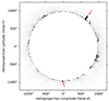 |
Fig. 1. SDO/AIA 304 Å image recorded on 6 June 2010 at 15:00:00 (UT time) and pre-processed by the procedure developed by Liu et al. (2023). Here the inverted image is displayed instead of the original image for visualisation purposes. The red arrows indicate solar jets (checked manually). |
2.2. Mathematical morphology
Mathematical morphology is an image processing method, built on set theory, which consists in analysing, extracting or detecting image features by comparing them with simpler feature shapes. With this method, one is able to compare the complex-shaped objects in images with a smaller and simpler-shaped object – the structuring element (SE). The image is processed based on this SE and a MM function enabling the extraction of complex features. In other words, the SE scans the image – similarly to a kernel in a convolution operation – and modifies the features of the images in accordance with one determined MM transform. A combination of multiple SEs can be used as parameters in each transform to enhance the desired results, as demonstrated by Lirui & Runtao (1991). According to the image dimensions and type, and to the MM function that one considers applying on to the image in line with one’s purposes (e.g. noise filtering, edge detection, feature segmentation, image enhancement), the user pre-defines a suitable SE. The SE is indeed a highly customisable object as one has a free hand on varying its shape, size, and orientation altogether. In addition to the SE, MM stands on two fundamental functions that we briefly introduce: erosion and dilation. Erosion is denoted and defined in Eq. (1) (Soille 1999) from the perspective of set theory, with S designating the SE and X a set:

The erosion of X by S consists in all the points x such that the SE (which origin is at x) entirely fits in X. In the images, this erosion operation results in shrinking objects’ boundaries, as Eq. (2) (Soille 1999) shows. The dilation, on the other hand, is described in Eq. (3) (Soille 1999) and contains all points x such that the SE (with origin at x) hits X in some way:

The dilation operation thus entails an expansion of objects’ boundaries in images (see Eq. (4)). By combining and chaining these two basic operations, more complex transformations can be created; for instance, the following functions, white top-hat, morphological opening and gradient, respectively:
![$$ \begin{aligned} \gamma _{S}(f)&= \delta _{S}[\epsilon _{S}(f)], \end{aligned} $$](/articles/aa/full_html/2025/01/aa51257-24/aa51257-24-eq6.gif)
In this work we seek to apply MM functions on the pre-processed satellite data introduced earlier in Sect. 2.1 in order to extract all the coronal off-limb structures visible in these images. Figure 2 displays the main steps of our processing algorithm.
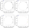 |
Fig. 2. Main steps of the extraction algorithm applied to the image described in Fig. 1. The images are inverted for visualisation purposes. Panel A: White top-hat operation. The small, bright features of the image (here highlighted in black) smaller than 200 pixels (the size of the SE used in this operation) are isolated. Panel B: Fixed threshold. The image is binarised. Panel C: Small object removal function. Noise smaller than 5 pixels (the SE size) is eliminated, retaining only the structures of interest. Panel D: Labelling. Each coronal off-limb structure is labelled with a unique number and colour. |
First, we perform a white top-hat operation (Fig. 2A), which is defined in Eq. (5) as the difference between the image and its opening γ. γ is described in Eq. (6) (Soille 1999). In practical terms, the opening function is a dilation of an erosion (with the same SE), that is, the image is partly reconstructed from the erosion by the dilation operation, leading to the removal of small objects while still preserving the larger structures in the original image. The opening is incorporated in the white top-hat operation which, as its name suggests, isolates small peaks (brightest regions) standing out in an image. Here, we resort to the white top-hat as we aim to uncover the bright coronal features – which are already emphasised by the pre-processing steps led by Liu et al. (2023) – instead of a black top-hat, based on the closing transform function, that highlights the small dark features such as sunspots (Bourgeois et al. 2024). The SE chosen for the top-hat transform is a circular object with a size of 200 pixels.
Subsequently, a fixed threshold of 135 was applied in Fig. 2B to create a binary image. This thresholding technique allows us to distinguish between the coronal off-limb structures and the background noise by establishing a specific value that separates the bright features from the darker areas. In the resulting binary image, the inverted bright pixels (shown in black) represent the areas of interest. Following this, in Fig. 2C, a small object removal function was utilised with a circular SE of 5 pixels. This step is crucial for enhancing the quality of the image by eliminating small-sized noise that does not correspond to the coronal structures. By using a circular SE, we ensure that any isolated pixels or small groups of pixels smaller than 5 pixels are removed, allowing us to retain only the larger, meaningful coronal off-limb structures that we are interested in analysing. Finally, in Fig. 2D, each coronal off-limb structure is assigned a unique label, facilitating identification and reference throughout the analysis. In total, 53 distinct coronal off-limb structures are identified in this image.
We then apply a morphological half-gradient by dilation – also referred to simply as external gradient – to extract the labels’ contours. The external gradient is the difference between the dilated image and the image itself (see Eq. (7)) and is indeed very helpful in underlining objects’ edges within an image. In Fig. 3, the coronal feature contouring – elicited through the external gradient – is overlaid on the pre-processed image that has been disposed of all the white noise (here appearing in dark in the inverted image). The contours have been eroded with a circular SE of size 2.5 in order to distinguish the inner structures with more clarity.
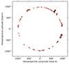 |
Fig. 3. Contouring of all the coronal off-limb structures (obtained via application of the morphological gradient operation) overlaid on the pre-processed image from Fig. 1 (6 June 2010 at 15:00:00 UT time) after noise filtering. We show the inverted image. |
The main steps of this algorithm (Fig. 2) have automatically been reiterated on all the images of the dataset (Sect. 2.1). The different values of the threshold and MM function parameters are described in the previous paragraphs of this section. For each MM transform, we use a disk-shaped SE so as not to distort the solar disk and to keep isotropic features; however, we note that if our aim were to detect coronal jets only, a line-shaped SE would prove more suitable to the identification of these straight-like structures. It is important to mention here that we did not discriminate between the short- and long-lived coronal off-limb structures: some of them last more than three hours but are to be identified by the algorithm as new structures.
3. Properties
Once we extracted all coronal off-limb structures, we were able to proceed with the computation of their main characteristics such as their area (in square megametres, Mm2), perimeter (in megametres, Mm), length (Mm), width (Mm). The length and width of the structures were computed using the Feret diameter. Defined, for instance, by Lourenço et al. (2015), the Feret diameter consists of a set of distances between any two parallel tangents to the structure’s contour (similar to a slide gauge measurement); the length and width are thus represented by the maximum and minimum Feret diameter, respectively. We also measured the position angle (PA) of the coronal structures’ central points (calculated anticlockwise from the solar north pole, in degrees) and, from there, we derived the centroids’ longitude and latitude – without correction for the B0 angle. The B0 angle represents the heliographic latitude of the solar disk centre and oscillates in a sinusoidal manner between −7, 23° and +7, 23° when observed from the Earth. We consider it to be negligible in this work.
Moreover, the MM library that we use for quantitative image analysis, DIPlib, enables us to calculate various morphology parameters including circularity, convexity, eccentricity, Podczeck shapes, mean radius of structures. We do not describe them thoroughly here as our statistical study focuses mostly on the other properties mentioned above, as well as on the intensity behaviour of the coronal features. However, all properties can be found in the dataset available on the University of Sheffield’s Online Research Data (ORDA) repository1.
The intensity is assessed in digital number (DN) and corrected for the charge-coupled device (CCD) sensitivity degradation on board the SDO/AIA instrument with the aiapy package tool developed by Barnes et al. (2020). Notwithstanding this correction, the intensity measurement seems to suffer from this degradation and early on since the launch of the SDO spacecraft in 2010, as seen in Fig. 4.
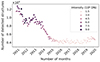 |
Fig. 4. Monthly distribution of the density and intensity of coronal off-limb structures from 1 January 2011 00:00:00 to 31 December 2021 21:00:28 UT. The structures were recorded at three-hour intervals, and the total number observed each month is displayed on the y-axis. Each dot represents the total number of observed structures per month, with the size and colour of the dots indicating their intensity. Smaller and lighter dots correspond to weaker summed intensities, while larger and darker dots represent higher summed intensities. The intensity and number of detected structures are correlated. A peak in both density and intensity occurs in 2013, while the overall trend shows a sharp decline throughout SC 24, with a slight increase at the beginning of the next cycle around 2019–2020. |
Figure 4 displays the monthly distribution of coronal off-limb structures. Both the markers’ size and colour indicate the coronal off-limb structures’ intensity (corrected for the CCD degradation): darker and larger data points represent the coronal off-limb structures with higher intensity values (in DN) while lighter and smaller data points show lower intensities. The influence of the solar cycle is conspicuous: the peak in the number of coronal features at the start of 2013 depicts the solar cycle approaching its maximum, and both the intensity and the density of features slightly increase in 2019, as a new solar cycle – SC 25 – begins its expansion (starting in December 2019). However, the number of features strikingly decreases with time. Likewise, the features’ intensity follows a declining trend overall. Despite the correction for the CCD degradation, the impact of the latter on the pixel intensities – also acknowledged by Ahmadzadeh et al. (2019) – remains far too important, especially in the AIA 304 Å passband (forming at temperatures around 50 000 K), as it has been spectacularly evidenced by Zwaard et al. (2021). This effect is thus to be kept in mind all along our statistical interpretations in the next section.
4. Statistical results
The statistical results obtained from the extraction of 877 843 coronal off-limb structures (described in Sect. 2) for nearly the entire duration of SC 24 (June 2010–December 2021) are presented here. Beforehand, the number of structures will be examined against latitude.
4.1. North–south asymmetry
Figure 5 shows the kernel density estimate (KDE) plot of the latitude of all the detected coronal off-limb structures. KDE is a non-parametric method yielding an estimation of features’ density based on so-called kernels that act as weights balancing up the distances of all data points. In Fig. 5, the edge effects have been discarded by rolling up the KDE distribution (i.e. the same distribution has been prior and subsequently appended). Two clear peaks stand out at mid-latitudes around ±20/25°, as one might expect it. There are fewer coronal features near the solar poles, but the more we progress towards the mid-latitudes, the more these features become abundant. After reaching a local maximum at ±20/25°, the number of coronal structures decreases again while approaching the equator – a dip is visible at 0°. Interestingly, we observe that the two maxima are not of equal height: the north features a higher density of coronal features at +20/25° with a maximum at a density of 3, 17 × 10−3 against a maximum at a density of 2, 91 × 10−3 in the south. This observation seems to reveal the so-called N-S asymmetry.
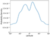 |
Fig. 5. Latitudinal distribution of coronal off-limb structures during SC 24. Two prominent peaks are observed at latitudes around +20/25° and −20/25°, corresponding to the active latitude belts. A slight gap between these peaks may suggest a N-S asymmetry, with a subtle predominance of activity in the northern hemisphere during this cycle. |
Figure 5 shows a northern dominance during Solar Cycle 24 that is also supported by the findings of Chandra et al. (2022). In their case, in the periodicity of the daily sunspot number, they also reported a southern dominance during SCs 22 and 23. Other authors found, instead, increased solar activity in the southern hemisphere during SC 24 (e.g. Liu et al. 2023 with coronal jets). There is some inconsistency about this topic in the literature. For example, Hao et al. (2015) observed a southern dominance during SC 22 followed by a northern dominance in SC 23 and during the rise of SC 24 (but their study ends in December 2013), which is contradictory with the works of Li et al. (2009) and Chandra Joshi et al. (2009) who reported a southern dominance during SC 23 in sunspot activity and prominences, respectively.
These discrepancies between different studies may come from the variety of observed solar features (e.g. sunspots, filaments, prominences, jets) which exhibit distinct behaviours due to the influence of localised small-scale dynamics. Coronal off-limb structures are no exception as they encompass jets and prominences along with other features that may follow a different trend to that of sunspots (see Fig. 8 in Sect. 4.2). In addition, the datasets in different studies might have been created in a different manner. We recall here that our dataset contains structures that may be registered more than once (in fact, all structures living longer than three hours), which can introduce some bias. Hao et al. (2015) face a similar difficulty with their filament database (with one-day cadence), while other authors count each structure only once (e.g. Liu et al. 2023 and their 1215 jets).
The N-S asymmetry thus seems to depend on the solar cycle, but also on the year (see Fig. 6) and even on the month (see Fig. 7). For instance, Fig. 6 showcases the KDE plot of the latitude of the coronal off-limb structures for each year of our dataset. We note that the first year (2010, first row) may not be entirely relevant here as it contains only half of the data (starting from June 2010). The KDE distribution has been rolled up as described previously to prevent any edge effect. We point out here that the KDE distribution is not normalised in Figs. 6 and 7, nor in any of the subsequent figures in this paper that show a KDE distribution. Consequently, the rows can be compared against each other qualitatively but not quantitatively. The bandwidth of the kernel function used in Fig. 6 and in the following KDE distributions is 0.5.
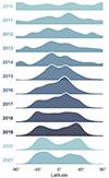 |
Fig. 6. Distribution of the latitude of coronal off-limb structures per year. Row 1 corresponds to 2010 and row 12 to 2021. Only six months of data were recorded in 2010, while the other rows represent entire years. This figure is consistent with the butterfly diagram, illustrating two distinct latitudinal peaks in the northern and southern hemispheres for most years. These peaks shift over time, moving closer to each other and toward the equator around the maximum of SC 24 in 2014 and at the beginning of the declining phase. Eventually, they converge into a single peak near the equator (slightly to the northern side). At the end of SC 24 and the beginning of SC 25, the peaks appear distinctly apart as coronal activity increases at mid-latitudes. |
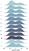 |
Fig. 7. Distribution of the latitude of coronal off-limb structures per month in 2021. Row 1 corresponds to January and row 12 to December. Notably, the two expected peaks in latitude (corresponding to the active latitude belts) are not consistent across the hemispheres throughout the months, revealing a strong N-S asymmetry. There is a predominance of coronal activity in the southern hemisphere at the beginning and end of the year, while the northern hemisphere exhibits either equal or greater coronal activity during the middle of the year. |
From Fig. 6, it is clear that the north mostly dominates during SC 24, barring the coronal activity prevalence of the southern hemisphere in 2013–2014 and 2020–2021. These observations are consistent with the study carried out by Zhang et al. (2024) on active regions: they found a southern predominance in 2012–2015 and 2020. In our case, it is more uncertain to find any prevailing activity regarding the years 2012 and 2015 as peaks in both hemispheres seem to be at approximately the same height. We also notice that coronal activity in the northern hemisphere is so preponderant at the beginning of the declining phase of SC 24 (2016–2017) that we almost see only one peak in the distribution. Around the solar minimum, the active latitudes – appearing where the solar activity is more intense – shift considerably. At the minimum of SC 25 (reached around 2019), the two peaks – located at ±40/45° – are separated by almost 90°. Although the active latitudes around the solar minimum are usually closer to the equator (around ±20/30° instead of ±40/45°), the butterfly diagram and its N-S asymmetry is quite well represented here in the case of coronal off-limb structures.
The N-S asymmetry is also illustrated by the time-distance plot in Fig. 7, where each row corresponds to a month in 2021 (starting with January in row 1). In this year, coronal activity is more pronounced in the southern hemisphere, particularly at the beginning and end of the year. A slight predominance of coronal feature density is observed in the northern hemisphere during June, July, and August, suggesting that the N-S asymmetry fluctuates on a monthly timescale. Interestingly, a roughly four-month cycle appears, with coronal activity alternating between the southern and northern hemispheres. This pattern bears a notable resemblance to the Rieger period, which spans approximately 158 days and has been observed in several solar phenomena, including sunspots and solar flares (Rieger et al. 1984). Further analysis of monthly distributions from other years reveals different patterns, such as a stronger northern hemisphere predominance in some years. These month-to-month variations are crucial for understanding solar dynamics and predicting solar activity, as they reflect the complex interactions between the Sun’s magnetic field and coronal structure density. Periods of heightened activity in one hemisphere increase the likelihood of solar eruptions in that region, which can, in turn, impact space weather conditions in different areas of space, including Earth.
4.2. Intensity behaviour
We now continue to explore the distribution of coronal structures with regard to latitude – namely the butterfly diagram, and its active latitudes – but now with a specific focus on the intensity behaviour of these structures (bearing in mind the decline of intensity due to the CCD degradation mentioned in Sect. 3). The latitude of the coronal off-limb structures is plotted as a function of time in Fig. 8. The colour bar indicates the intensity of these structures, spanning the DN range of [103, 106]. The intensity is then normalised on a log scale to the [3, 6] range, which enables us to distinguish qualitatively more clearly between low-intensity (blue-ish dots), medium-intensity (green-ish dots), and high-intensity (red-ish dots) structures.
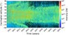 |
Fig. 8. Latitude and intensity of coronal off-limb structures as a function of time. The intensity of the coronal structures in digital number (DN) is represented using a gradual colour-code based on a logarithmic scale, with blue indicating the lowest-intensity structures and red indicating the highest. The distribution of structures per latitude over time clearly illustrates the butterfly diagram (particularly when looking at the highest-intensity reddish structures), with coronal activity moving toward the equator as SC 24 progresses. It also shows the notable rush-to-the-poles phenomenon observed in both hemispheres between 2010 and 2015, with several surges in the northern hemisphere. |
Intriguingly, the butterfly diagram is here essentially generated by the coronal structures with higher intensity (in red) that seem to markedly follow the solar magnetic cycle; the butterfly wings are well shaped by the high-intensity structures starting to appear at latitudes around ±20° between 2010 and 2012, and progressively decreasing towards lower latitudes as the solar cycle evolves with time. A very high density of these red-ish structures can be observed between 2014 (year in which the solar cycle reaches its maximum) and 2016. This number then substantially decreases after that time (i.e. during the descending phase of SC 24 and the very beginning phase of SC 25 starting in 2019). The butterfly wings make an appearance again as more high-intensity coronal structures re-emerge in 2021 with SC 25 beginning its ascent. Figure 8 shows thus the butterfly diagram as anticipated; however, only for the coronal structures with higher intensity. The lower- and medium-intensity structures exhibit a more dispersive behaviour; we also note a higher density of these structures during the declining phase of SC 24 in contrast with that of higher-intensity structures.
Coronal structures with medium intensity (in green) manifest an interesting behaviour with long-shaped green-ish structures heading from high-latitude regions towards the solar poles – known as the ‘rush-to-the-poles’ phenomenon occurring just before the polar magnetic field reversal due to the solar cycle evolution (Lockyer 1931; Hyder 1965; Yeates 2013). In recent works referring to SC 24, the rush-to-the-poles structures have been evidenced in the same kind of plot, for example by Diercke et al. (2024) with solar filaments and by Zhang et al. (2024) with prominences. Yeates (2013) also found similar structures during SC 23 by simulating the latitude distribution of flux ropes.
The N-S asymmetry is once again accentuated by the visible offset in the migration of these high-latitude structures to the poles between both hemispheres (Diercke et al. 2024). The rush-to-the-poles in the northern hemisphere starts in 2010 and seem to end in 2013 (although a second structure arises from 2013 to 2015), while the rush-to-the-poles in the southern hemisphere begins later, in 2012, and finishes in 2015, indicating that the polar field reversal takes place one year after the solar maximum in the south (but also in the north if we count what appears to be a second rush-to-the-poles surge).
The observation of this two-year offset between hemispheres complies with the findings of Zhang et al. (2024), whereby they found that the occurrence of both active regions and prominences reached its summit in 2011 in the northern hemisphere and in 2013 in the southern hemisphere, respectively. Gopalswamy et al. (2016) also found various rush-to-the-poles surges in the northern hemisphere in terms of prominence eruptions, whilst the rush-to-the-poles structure in the southern hemisphere shows a steadier pattern. However, they determined that the rush-to-the-poles phenomenon lasts longer in the north (until the end of 2015 against 2014 in the south). They thus derived that the magnetic field reverses later than expected (after the solar maximum) and that SC 25 might be delayed in the northern hemisphere. In the past solar cycles, the magnetic field reversal was always to happen first in the north (Gopalswamy et al. 2016); regarding SC 25, Jha & Upton (2024) also predicted the magnetic field reversal to arise first in the northern hemisphere and, only a few months later, in the southern hemisphere. In Fig. 8, the northern and southern rush-to-the-poles seem to end at around the same time, in 2015 (by taking into account the second poleward structure in the north).
After the magnetic field reversal, we notice that there is still a high density of medium-intensity features during the descending phase of SC 24 at high latitudes around ±40/50°, which reveals a continuous activity from these features. Therefore, the butterfly shape is not clear in regards to lower-intensity coronal off-limb structures, while the high-intensity coronal structures are distinctly modulated by the solar cycle evolution, as illustrated by Figs. 8 and 9.
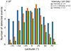 |
Fig. 9. Number of detected coronal off-limb structures as a function of latitude. The different colours account for three categories of intensity (low-intensity structures in blue, medium-intensity structures in orange, and high-intensity structures in green). |
Figure 9 displays the number of coronal off-limb structures as a function of latitude with 11 bins. Information about the intensity of the structures is provided by the colour-code employed in this plot: in blue, we show the structures with an intensity lower than 20 000 DN (388 936 structures); in orange, the structures are with an intensity between 20 000 and 55 000 DN (280 513 structures); in green, the structures are with an intensity above 55 000 DN (208 394 structures). Here, again, the active latitudes are conspicuous at around ±20°, for all three categories of intensity. Nevertheless, the lower-intensity coronal structures (in blue) seem once more to follow a different pattern in comparison with the higher-intensity structures (in orange and green). We observe a large number of lower-intensity structures at high latitudes between −90° / − 50° and 50° /90°, which is highly supported by the distribution of the blue and green dots in Fig. 8 and complementary to the characteristic trend of the blue curve in Fig. 10.
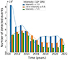 |
Fig. 10. Number of detected coronal off-limb structures as a function of time. The legend is the same as in Fig. 9 (blue: low-intensity structures; orange: medium-intensity structures; green: high-intensity structures). |
Figure 10 shows the number of coronal off-limb structures as a function of time. The colour-code is the same as in Fig. 9. The declining phase of SC 24 is marked by a salient increase of lower-intensity structures after a local maximum in 2013 and a local minimum in 2015, while the number of medium- and high-intensity features decreases in accordance with the evolution of the solar cycle. A curious peak in the number of lower-intensity features stands out in 2010; it might be due to the CCD degradation (see Sect. 3) as the fainter structures were more accurately recorded in 2010 (and thus captured by the MM detection algorithm) by the AIA instrument that was, very quickly after the launch of the SDO satellite, strongly affected by its CCD sensitivity degradation.
The peculiar behaviour exhibited by low-intensity coronal off-limb structures – namely, the increase in the number of these features during the decaying phase of SC 24, as depicted in Figs. 8 and 10 – may also be a consequence of CCD degradation. Yet, other studies have reported similar behaviour for certain types of features, such as isolated sunspots, which appear more frequently than expected during the decaying phase (Koutchmy & Le Piouffle 2009). Zhang et al. (2024) also observed a related trend in prominence areas: only prominences with a large projected area (> 4.103 Mm2) seem to clearly follow the solar cycle evolution, while the number of small- and medium-area prominences expands during the declining phase of SC 24 – similarly to the low-intensity coronal off-limb structures in our dataset. However, we only found this pattern when investigating the intensity of these structures. In terms of projected area, we did not uncover a similar trend concerning the small-area structures – the solar cycle variations modulate the density of coronal off-limb structures in all categories of area, without exception.
In conclusion, the intensity behaviour of the coronal off-limb structures is challenging to interpret due to the lack of information about the specific types of coronal structures (e.g. jets, loops, prominences) contributing to each intensity category. Moreover, we cannot ascertain whether we are observing the early, intermediate, or late stages of these structures’ evolution, each of which significantly affects their observed intensity. Although the temporal and latitudinal behaviour of coronal off-limb structures appears to vary across different intensity categories (as shown in Figs. 8, 9, and 10), the overall trend remains relatively consistent. Specifically, the distribution across latitude follows a pattern similar to the well-known butterfly diagram and can be approximated by a double-peaked Gaussian distribution, as evidenced in Fig. 9.
The main distinction lies in the behaviour of lower-intensity features, which tend to display a wider distribution across latitudes. A notably high density of low-intensity structures is observed at high latitudes, which is consistent with the findings on polar jets – smaller and fainter jets typically found near the poles. Soós et al. (2024) reported that polar jets are less intense but more frequent compared to their lower-latitude counterparts, which are generally larger and more energetic. This wider distribution of weaker-intensity features may reflect the prevalence of these smaller-scale events in polar regions, contributing to the overall complexity of the observed intensity trends.
4.3. Active longitudes
The latitudinal distribution of coronal off-limb structures complies with the solar cycle evolution (at least in terms of high-intensity structures) and results in the emergence of long-established active latitudes, latitudes where the solar activity is magnified, and that were first brought to light through historical sunspot recording. The questions arise, however, about the longitudinal distribution of coronal off-limb structures, how it is shaped, and whether it follows a cyclical pattern, as its latitudinal counterpart does. We address these questions in what follows.
The longitudinal distribution of solar activity (including sunspots, flares, CMEs) has been studied for many years (Chidambara Aiyar 1932; Bogart 1982; Bai 1987) and is known to be non-uniform, with magnetic features clustering in two preferred longitudinal positions approximately 180° apart, hence the term ALs. These ALs have been observed to maintain a relatively constant position (with a 26° dispersion over 10 solar cycles; see Plyusnina 2010), although they are subject to the “flip-flop” effect – a periodic switch in the dominant longitudinal position of solar activity observed first in starspots (Jetsu et al. 1991; Elstner & Korhonen 2005). ALs have been detected on other stars (Berdyugina et al. 2002; Lanza et al. 2009) and in various solar features. For example, Berdyugina & Usoskin (2003) investigated ALs in sunspots over 120 years, while Gyenge et al. (2012) used the Debrecen Photoheliographic Data (DPD, Baranyi et al. 2016; Győri et al. 2017) to explore the longitudinal behaviour of active regions between 1979 and 2011 in the northern hemisphere. ALs have also been thoroughly examined in the distribution of CMEs (Skirgiello 2005; Gyenge et al. 2017), coronal streamers (Li 2011), the interplanetary magnetic field (Neugebauer et al. 2000), and solar flares (Bumba & Obridko 1969; Heras et al. 1990; Mordvinov et al. 2002; Zhang et al. 2007). Specifically, Zhang et al. (2008) found that 80% of C-class flares occur in ALs (±20 − 30°) around solar minimum, and 80% of X-class flares occur in ALs (±20 − 30°) at solar maximum. Later, Gyenge et al. (2016) discovered that ALs (±36°) enclose more than 60% of the flares detected by GOES and the Reuven Ramaty High Energy Solar Spectroscopic Imager (RHESSI). Consequently, the position of ALs is an important proxy for improving solar flare forecasting, as demonstrated by Huang et al. (2013), who used the distance between active regions and ALs as a valuable parameter to upgrade the performance of their flare forecasting model.
According to Usoskin et al. (2007), ALs are influenced by two main factors: differential rotation and the latitudes of intense solar activity (i.e. active latitudes). ALs rotate differentially in both hemispheres, resulting in a characteristic N-S asymmetry (Mordvinov & Kitchatinov 2004; Berdyugina et al. 2006; Zhang et al. 2011), which may stem from the so-called stroboscopic effect (illustrated by Usoskin et al. 2007). This effect induces the motion of a non-axisymmetric, quasi-rigid magnetic structure – responsible for the emergence of ALs – when it is enlightened by a dynamo (axisymmetric) wave propagating toward the solar equator. Kitchatinov & Olemskoi (2005), Olemskoy & Kitchatinov (2009) support the idea that AL formation is linked to the presence of a rigid background magnetic field embedded in the uniformly rotating radiative zone. Specifically, ALs may arise from the interaction between cyclically oscillating axisymmetric dynamo modes and a non-axisymmetric relic field, which weakly but consistently modulates the global mean magnetic field (Mordvinov et al. 2002; Jiang & Wang 2007; Raphaldini et al. 2023). Dikpati & Gilman (2005), Dikpati et al. (2018), Dikpati & McIntosh (2020) discuss the magnetohydrodynamics (MHD) shallow-water model at the base of the convection zone (i.e. the tachocline) and show that stationary (or quasi-stationary) Rossby waves can lead to flux emergence by forming bulges of toroidal field at preferred longitudes after interacting with differential rotation instability and toroidal fields within the tachocline.
However, the theory behind ALs remains unclear. ALs can be difficult to detect, vary across solar cycles, and appear more acutely in certain solar features than in others. For example, Zhang et al. (2007) observed that X-ray flares are more frequently detected in ALs compared to sunspots. Therefore, it is essential to investigate ALs across various solar structures and over extended periods to ascertain their long-lived existence. While longitudinal inhomogeneities in solar activity are generally accepted, studies differ on their exact location, rotation rate, and lifespan, often due to differences in the methods used for detection (Berdyugina & Usoskin 2003). For instance, Pelt et al. (2005) questioned Berdyugina & Usoskin (2003)’s findings, suggesting that their data processing introduced a bias, leading to a bimodal distribution irrespective of the initial distribution (whether randomly generated or real sunspot longitudinal distribution).
In this work, we measure the Carrington longitude at the centroids of all the coronal off-limb structures contained in our dataset (877 843 spanning SC 24). Figure 11 shows the number of these coronal structures distributed as a function of Carrington longitude. We set to use 18 bins, that is, each bin spans 20° in longitude. That value has been used in previous works (Berdyugina & Usoskin 2003; Liu et al. 2023) in order to visualise better the ALs. The colour-code is the same as in Figs. 9 and 10. The coronal structures within all three categories of intensity seem to follow the same distribution. What stands out in this graph is a spatially periodically pattern with two peaks at around 100 and 200°; however, we are not able, as for now, to interpret this observation. ALs might be likely to appear in the distribution of coronal off-limb structures, but one would expect a separation distance of about 180° between each other. There are too many data points to visualise clearly any trends; we thus need to focus on shorter time ranges (e.g. of the order of months).
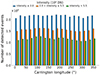 |
Fig. 11. Number of detected coronal off-limb structures as a function of Carrington longitude. The legend is the same as in Figs. 9 and 10 (blue: low-intensity structures; orange: medium-intensity structures; green: high-intensity structures). |
The KDE distribution of coronal off-limb structures per month as a function of Carrington longitude is displayed in Fig. 12. Similarly to Fig. 7, each row corresponds to the distribution over one month of the year 2021. We selected the year 2021 as this enables us to gain insight into the longitudinal distribution of coronal features during the rising phase of SC 25 – when solar activity begins to strengthen. For each month, we can see several peaks of density in the Carrington longitude distribution. Some of these peaks are plainly separated by 180°: January (row 1), June (row 6), July (row 7), August (row 8), September (row 9), October (row 10), and December (row 12) 2021. We notice an east–west (E-W) asymmetry in the peak height for some months; for example, that is particularly obvious in December, but also in March, August, and November 2021. Very interestingly, when looking at these monthly plots as a whole, we spot a shift of the crests across the months. One can easily follow all the crests from the one starting in row 1 at 360° down until the crest of row 9 or 10 at 0°, or else the one starting at 360° in row 6 down until the crest at about 160° in row 10. The motion of these crests looks consistent with an almost constant velocity, but this needs to be looked into further. We have here plotted the KDE distribution per month, but ALs last in general longer than a Carrington rotation: some months may display twice the same longitudes and introduce a bias in the distribution.
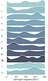 |
Fig. 12. Distribution of the longitude of coronal off-limb structures per month in 2021. Row 1 corresponds to January and row 12 to December. Notably, there are significant longitudinal peaks of coronal activity, with approximately one to three peaks occurring each month. These peaks exhibit a gradual shift in longitude over time. |
We show the difference by reproducing in Fig. 13 the plot of Fig. 12 every 27 days (instead of a monthly breakdown), which corresponds to the Bartels’ rotation. The Bartels’ rotation (exactly 27 days) is very close to the Carrington rotation but takes into consideration the apparent rotation of the Sun from the Earth’s viewpoint. Curiously enough, the divergence between Figs. 12 and 13 is substantial. The crests in Fig. 13 are less sharply shaped; for some months, several peaks are visible, sometimes very close to each other – the evidence for the 180° distance separation between ALs completely disappears. Nonetheless, one can still visualise a strong pattern; this time, not by following the crests but the dips. For instance, there are successive dips from row 2 to row 5 between 250° and 0°. The dips then shift and reappear from row 5 to row 9 between 300° and 180°, to finally relocate from row 10 to row 13 between approximately 50° and 150°. This dip displacement (that becomes a peak displacement in other years) reveals the zones of quiet longitudes and thus the dynamics of ALs. The discrepancies between the two Figs. 12 and 13 are due to the somewhat skewed nature of the monthly distribution of longitude. Because the Carrington rotation occurs approximately every 27 days, certain longitudinal zones are counted twice within a single month. In the case of a uniform distribution, this bias gradually propagates over time, leading to the formation of recurring peaks at specific longitudes that shift each month. In Fig. 12, we observe this pattern, but it is not as distinct as described, given that the longitudinal distribution is not uniform. Hence, the importance of examining this distribution over a 27-day period.
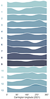 |
Fig. 13. Distribution of the longitude of coronal off-limb structures per Bartels’ rotation in 2021. Row 1 corresponds to the KDE distribution over the first 27 days of the year. Longitudinal peaks are present, but are less consistently regular compared to Fig. 12, as this distribution is not influenced by the bias introduced by monthly divisions. Instead, the apparent rotation of the Sun, as seen from Earth, is accounted for. |
However, the longitudinal inhomogeneities in Fig. 13 are smoothed out as the distribution is plotted across all latitudes. Usoskin et al. (2007) found that ALs undergo the effects of differential rotation, but also of variations in solar activity at different latitudes. The Carrington rotation represents the average rotation rate of the Sun, while the regions actually rotating with a 27-day period are situated around 40° and −40° latitude. In contrast, the equatorial region, for instance, rotates with a 25-day period. It is thus crucial to investigate the longitudinal distribution of coronal off-limb structures within specific latitude bands whose rotation period aligns with the chosen period in the displayed distribution.
In Fig. 14a, we present the 27-day longitudinal distribution of coronal off-limb structures selected within a 10° band centred around +40° in the northern hemisphere and −40° in the southern hemisphere. We then plot this same distribution separately for each hemisphere in Figs. 14b and 14c to compare them and examine potential patterns of the N-S asymmetry. When simultaneously looking at both hemispheres in Fig. 14a, we note the presence of one or several peaks in each 27-day period. Some are clearly separated by a distance close to 180°, for example, in row 2 around 135° and 315° longitude, in rows 5 and 11 around 150° and 330°, and in rows 6, 7 (very similar), and 9 around 0°, 180°, and 360°. The ALs are now much easier to identify within a specific latitude belt. The peaks are distinct and migrate over time. For example, from row 1 to row 7, there is a peak between 270° and 360° that eventually disappears, making way for another prominent peak visible from row 5 to row 9 around 180° longitude. Another peak emerges from row 9 to row 12 and progressively shifts with time between 0° and 180°.
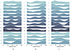 |
Fig. 14. Distribution of the longitude of coronal off-limb structures over a 27-day period in 2021, shown for different latitude belts: centred around 40° in the northern hemisphere (panel b) and −40° in the southern hemisphere (panel c), with a latitude range of ±5°. Panel (a) shows the longitudinal distribution simultaneously centred around 40° latitude in the northern hemisphere and −40° latitude in the southern hemisphere, also with a latitude range of ±5°. These latitude belts correspond to the solar regions rotating with an approximately 27-day period, while lower latitudes rotate faster and higher latitudes rotate more slowly. (a) Latitude belt at ±35°/±45°. (b) Latitude belt between 35° and 45°. (c) Latitude belt between −45° and −35°. |
In Fig. 14a, we also notice a greater contribution to longitudinal irregularities from the southern hemisphere as it manifests higher activity in 2021 compared to the northern hemisphere (see Fig. 7). When focusing only on the 40° latitude belt in Fig. 14b, we can discern two peaks separated by about 180° in most rows. However, the distance between these peaks varies, occasionally being closer or farther apart than 180°. Particularly noteworthy is the significant discrepancy in height between these two peaks (for example, from row 2 to 7 around 140° and 320° longitude), indicating a pronounced E-W asymmetry that may reveal the “flip-flop” phenomenon. The distribution in the southern hemisphere (see Fig. 14c) appears to be more dynamic. It occasionally exhibits only one peak, while in certain rows such as rows 1, 6, 7, and 9, it may display three peaks. In these rows, two peaks are sometimes very close to each other and distant from the third one. In contrast, rows 3 and 4 distinctly show two peaks separated by approximately 180°. In row 4, the peaks are of equal height, occurring around 90° and 270°, whereas in row 3, there is an E-W asymmetry between the peaks at about 130° and 310°.
Interestingly, we observe that in certain rows, a decline in coronal activity in the northern hemisphere corresponds to an increase in activity in the southern hemisphere, and vice versa. For instance, in row 0, a dip is observed in the northern hemisphere around 90°, while a significant peak emerges at the same longitude in the southern hemisphere. Similarly, in rows 3 and 10, a dip around 120° in the northern hemisphere corresponds to a peak in the southern hemisphere. In row 2, a peak appears between 270° and 360° in the northern hemisphere, while a large crest extends from 0° to 180° in the southern hemisphere. In row 4, there is a peak in the north around 320°, while peaks in the south are situated around 90° and 270°. In row 11, a peak around 160° is observed in the northern hemisphere, and another peak in the southern hemisphere is approximately at 340°, resulting in two distinct peaks separated by about 180° in Fig. 14a. Regarding the three peaks (located around 0°, 180°, and 360°) seen in rows 6 and 7 in Fig. 14a, they also arise from different peak locations in both hemispheres that complement each other. Therefore, it is essential to account for the N-S asymmetry when investigating ALs and to analyse each hemisphere separately, as the ALs exhibit an offset between the two hemispheres.
For comparison, we display in Fig. 15 the longitudinal distribution of coronal off-limb structures for the same year (2021), but this time centred around the equator and displayed with a 25-day period accordingly. Figure 15a illustrates the distribution within a 10° latitude band centred around the equator (0°), whereas Fig. 15b concentrates on the northern hemisphere (latitude belt between 0° and 5°), and Fig. 15c on the southern hemisphere (latitude belt between −5° and 0°). The effects of the N-S asymmetry are less pronounced in this case, given the equatorial distribution. The three figures appear to be very similar, with peaks mostly located at the same positions in both hemispheres. However, some variations are observed, such as in rows 5 and 6 where more peaks are visible in the northern hemisphere, and in rows 1, 2, 12, and 14 where an offset in peak locations occurs between the hemispheres. Overall, the presence of crests in Fig. 15a indicates the existence of ALs, although discerning the 180° separation distance between them is more challenging, except in rows 0, 5, and 6.
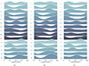 |
Fig. 15. Distribution of the longitude of coronal off-limb structures over a 25-day period in 2021, shown for different latitude belts centred around the equator. Panel (a) shows the longitudinal distribution centred around 0° latitude with a range of ±5°, while panel (b) displays the longitudinal distribution over the northern part of this belt (0° to 5° latitude), and panel (c) over the southern part (−5° to 0° latitude). |
5. Conclusion
In this paper we introduced a processing method based on MM transforms and applied it to the identification of coronal off-limb structures in SDO/AIA 304 Å images during SC 24 (starting in June 2010 and finishing in December 2021, with a three-hour cadence). After filtering (removal of noisy and misaligned images), the dataset contained 32 985 images with a total of 877 843 coronal off-limb structures. This high number of structures allowed us to carry out a statistical study by assessing their main characteristics (e.g. area, intensity, latitude, and longitude). Our main conclusions are summarised below:
-
The N-S asymmetry is strongly visible in the distribution of coronal off-limb structures (including in the rush-to-the-poles phenomenon) and varies according to the years and months due to the variations of the near-equatorial meridional circulation.
-
The rush-to-the-poles phenomenon is only observed with medium-intensity coronal structures (and not with high-intensity structures), probably due to the fact that this migration starts at high latitudes, while the lower-latitude structures also emit greater intensity.
-
Active latitudes (around ±20/30°) that shape the butterfly diagram are detected for high-intensity coronal structures. However, the distribution of the lower-intensity coronal off-limb structures does not show clear butterfly wings.
-
A high density of lower-intensity coronal structures appear at the high latitudes and solar poles, and during the declining phase of SC 24. This curious behaviour exhibited by the lower-intensity structures may be due in part to the CCD degradation of the AIA instrument.
-
We did not find a similar trend regarding the area of coronal structures, contrary to Zhang et al. (2024) who found that smaller-area prominences do not seem to follow the solar cycle evolution (only large-area prominences do).
-
In terms of ALs, we find a spatially periodically pattern in the longitudinal distribution of coronal off-limb structures.
-
The monthly distribution of the longitude of coronal off-limb structures, although nicely showing the peaks associated with ALs and occasionally the 180° separation distance between them, is skewed. As the Sun rotates with an average rotation period of 27 days, certain longitude bands may be counted twice.
-
We observe a strong drift of peaks and dips in the 27-day longitudinal distribution of coronal features that underline the dynamics of ALs.
-
However, considering the Carrington rotation alone is not sufficient, one must also account for the differential rotation occurring across different latitudes.
-
Plotting the 27-day longitudinal distribution within a 10° latitude belt centred around +40° and −40° reveals the existence of ALs, along with the blatant N-S asymmetry, as peaks in the southern hemisphere may align with the dips in the northern hemisphere and vice versa.
-
The 25-day longitudinal distribution of coronal off-limb structures within a 10° latitude belt centred around the equator also highlights the ALs, but the N-S asymmetry is less pronounced.
To achieve a deeper understanding of the statistics, conducting further investigations, particularly regarding the ALs, would be beneficial. One way to accomplish this would be to expand our database by including new images from multiple solar cycles, such as SC 25, or data from previous cycles obtained through other satellite sources, for example the Solar and Heliospheric Observatory (SOHO). Additionally, incorporating other SDO/AIA channels could help us identify certain corona aspects that may have been missed in the 304 Å wavelength channel. These efforts would lead to a more comprehensive and insightful data analysis. It is important to note that having too much data can sometimes make it difficult to identify clear trends in data distributions. To address this, it may be helpful to segment different coronal structures in our dataset. For instance, we used the 2704 labelled jets provided by Liu et al. (2023) and Soós et al. (2024) to identify coronal jets in our dataset. Other structures, for example prominences and loops, are also crucial to understanding solar phenomena and eruptions. Therefore, statistical studies of coronal structures are necessary and should be expanded.
Data availability
The dataset generated and analysed during the current study is publicly available in the ORDA (Online Research Data) repository of the University of Sheffield. It can be accessed at the following link: DOI: 10.15131/shef.data.27130590
Acknowledgments
This work is part of the SWATNet project funded by the European Union’s Horizon 2020 research and innovation programme under the Marie Skłodowska-Curie grant agreement No 955620. We acknowledge the use of the data from the Solar Dynamics Observatory (SDO). SDO is the first mission of NASA’s Living With a Star (LWS) program. The SDO/AIA data are publicly available from NASA’s SDO website (https://sdo.gsfc.nasa.gov/data/). TB and RG thanks for the support received from doi: 10.54499/UIDP/04434/2020 and doi: 10.54499/UIDB/04434/2020. J.L. acknowledges the support by the Strategic Priority Research Program of the Chinese Academy of Science (Grant No. XDB0560000), and the National Natural Science Foundation (NSFC 12373056, 42188101). R.E. is grateful to Science and Technology Facilities Council (STFC, grant No. ST/M000826/1) UK, acknowledges NKFIH (OTKA, grant No. K142987 and Excellence Grant TKP2021-NKTA-64) Hungary and PIFI (China, grant number No. 2024PVA0043) for enabling this research. MBK is grateful for the Leverhulme Trust Found ECF-2023-271. Sz.S. acknowledges the support (grant No. C1791784) provided by the Ministry of Culture and Innovation of Hungary of the National Research, Development and Innovation Fund, financed under the KDP-2021 funding scheme.
References
- Ahmadzadeh, A., Kempton, D. J., & Angryk, R. A. 2019, ApJS, 243, 18 [NASA ADS] [CrossRef] [Google Scholar]
- Bai, T. 1987, ApJ, 314, 795 [CrossRef] [Google Scholar]
- Bain, H. M., Copeland, K., Onsager, T. G., & Steenburgh, R. A. 2023, Space Weather, 21, e2022SW003346 [NASA ADS] [CrossRef] [Google Scholar]
- Baranyi, T., Győri, L., & Ludmány, A. 2016, ArXiv e-prints [arXiv:1608.08419] [Google Scholar]
- Barata, T., Carvalho, S., Dorotovic, I., et al. 2018, Astron. Comput., 24, 70 [NASA ADS] [CrossRef] [Google Scholar]
- Barnes, W., Cheung, M., Bobra, M., et al. 2020, J. Open Source Softw., 5, 2801 [NASA ADS] [CrossRef] [Google Scholar]
- Berdyugina, S. V., & Usoskin, I. G. 2003, A&A, 405, 1121 [NASA ADS] [CrossRef] [EDP Sciences] [Google Scholar]
- Berdyugina, S. V., Pelt, J., & Tuominen, I. 2002, A&A, 394, 505 [NASA ADS] [CrossRef] [EDP Sciences] [Google Scholar]
- Berdyugina, S. V., Moss, D., Sokoloff, D., & Usoskin, I. G. 2006, A&A, 445, 703 [NASA ADS] [CrossRef] [EDP Sciences] [Google Scholar]
- Blanter, E., & Shnirman, M. 2021, Sol. Phys., 296, 86 [NASA ADS] [CrossRef] [Google Scholar]
- Bogart, R. S. 1982, Sol. Phys., 76, 155 [NASA ADS] [CrossRef] [Google Scholar]
- Bourgeois, S., Barata, T., Erdélyi, R., Gafeira, R., & Oliveira, O. 2024, Sol. Phys., 299, 10 [NASA ADS] [CrossRef] [Google Scholar]
- Bumba, V., & Obridko, V. N. 1969, Sol. Phys., 6, 104 [NASA ADS] [CrossRef] [Google Scholar]
- Bumba, V., Garcia, A., & Klvaňa, M. 2000, Sol. Phys., 196, 403 [NASA ADS] [CrossRef] [Google Scholar]
- Canfield, R. C., & Pevtsov, A. A. 1998, ASP Conf. Ser., 140, 131 [NASA ADS] [Google Scholar]
- Carvalho, S., Gomes, S., Barata, T., Lourenço, A., & Peixinho, N. 2020, Astron. Comput., 32, 100385 [NASA ADS] [CrossRef] [Google Scholar]
- Castenmiller, M. J. M., Zwaan, C., & van der Zalm, E. B. J. 1986, Sol. Phys., 105, 237 [CrossRef] [Google Scholar]
- Chandra Joshi, N., Bankoti, N., Pande, S., Pande, B., & Pandey, K. 2009, Sol. Phys., 260, 451 [NASA ADS] [CrossRef] [Google Scholar]
- Chandra, Y., Pande, B., Mathpal, M. C., & Pande, S. 2022, Astrophysics, 65, 404 [NASA ADS] [CrossRef] [Google Scholar]
- Chidambara Aiyar, P. R. 1932, MNRAS, 93, 150 [CrossRef] [Google Scholar]
- Curto, J., Blanca, M., & Martínez, E. 2008, Sol. Phys., 250, 411 [NASA ADS] [CrossRef] [Google Scholar]
- de Toma, G., White, O. R., & Harvey, K. L. 2000, ApJ, 529, 1101 [NASA ADS] [CrossRef] [Google Scholar]
- Diercke, A., Jarolim, R., Kuckein, C., et al. 2024, A&A, 686, A213 [NASA ADS] [CrossRef] [EDP Sciences] [Google Scholar]
- Dikpati, M., & Gilman, P. A. 2005, ApJ, 635, L193 [NASA ADS] [CrossRef] [Google Scholar]
- Dikpati, M., & McIntosh, S. W. 2020, Space Weather, 18, e2018SW002109 [NASA ADS] [CrossRef] [Google Scholar]
- Dikpati, M., McIntosh, S. W., Bothun, G., et al. 2018, ApJ, 853, 144 [Google Scholar]
- Dodson, H. W., & Hedeman, E. R. 1968, Some Patterns in the Development of Centers of Solar Activity, 1962–66 (Dordrecht: Springer), 56 [Google Scholar]
- Elstner, D., & Korhonen, H. 2005, Astron. Nachr., 326, 278 [NASA ADS] [CrossRef] [Google Scholar]
- Gaizauskas, V., Harvey, K. L., Harvey, J. W., & Zwaan, C. 1983, ApJ, 265, 1056 [NASA ADS] [CrossRef] [Google Scholar]
- Georgoulis, M. K., Yardley, S. L., Guerra, J. A., et al. 2024, Adv. Space Res., in press https://doi.org/10.1016/j.asr.2024.02.030 [Google Scholar]
- Gopalswamy, N., Yashiro, S., & Akiyama, S. 2016, ApJ, 823, L15 [NASA ADS] [CrossRef] [Google Scholar]
- Green, L. M., Matthews, S. A., van Driel-Gesztelyi, L., Harra, L. K., & Culhane, J. L. 2002, Sol. Phys., 205, 325 [NASA ADS] [CrossRef] [Google Scholar]
- Green, L., Torok, T., Vrsnak, B., et al. 2018, Space Sci. Rev., 214, 46 [NASA ADS] [CrossRef] [Google Scholar]
- Gyenge, N., Baranyi, T., & Ludmány, A. 2012, Cent. Eur. Astrophys. Bull., 36, 9 [NASA ADS] [Google Scholar]
- Gyenge, N., Ludmány, A., & Baranyi, T. 2016, ApJ, 818, 127 [NASA ADS] [CrossRef] [Google Scholar]
- Gyenge, N., Singh, T., Kiss, T. S., Srivastava, A. K., & Erdélyi, R. 2017, ApJ, 838, 18 [NASA ADS] [CrossRef] [Google Scholar]
- Győri, L., Ludmány, A., & Baranyi, T. 2017, MNRAS, 465, 1259 [Google Scholar]
- Haas, A., Matheron, G., & Serra, J. 1967, Ann. Mines, 12, 767 [Google Scholar]
- Hao, Q., Fang, C., Cao, W., & Chen, P. F. 2015, ApJS, 221, 33 [NASA ADS] [CrossRef] [Google Scholar]
- Hathaway, D. 2010, Liv. Rev. Sol. Phys., 7, 1 [NASA ADS] [CrossRef] [Google Scholar]
- Heras, A. M., Sanahuja, B., Shea, M. A., & Smart, D. F. 1990, Sol. Phys., 126, 371 [NASA ADS] [CrossRef] [Google Scholar]
- Huang, X., Zhang, L., Wang, H., & Li, L. 2013, A&A, 549, A127 [NASA ADS] [CrossRef] [EDP Sciences] [Google Scholar]
- Hufbauer, K., & Dollfus, A. 2007, in In the Spirit of Bernard Lyot: The Direct Detection of Planets and Circumstellar Disks in the 21st Century, ed. P. Kalas, 17 [Google Scholar]
- Hyder, C. L. 1965, ApJ, 141, 272 [NASA ADS] [CrossRef] [Google Scholar]
- Iwanowski, M., Skoneczny, S., & Szostakowski, J. 1997, Int. Soc. Opt. Photon., 3164, 565 [Google Scholar]
- Janardhan, P., Fujiki, K., Ingale, M., Bisoi, S. K., & Rout, D. 2018, A&A, 618, A148 [NASA ADS] [CrossRef] [EDP Sciences] [Google Scholar]
- Jetsu, L., Pelt, J., Tuominen, I., & Nations, H. 1991, IAU Colloq., 130, 381 [NASA ADS] [Google Scholar]
- Jetsu, L., Pelt, J., & Tuominen, I. 1993, A&A, 278, 449 [NASA ADS] [Google Scholar]
- Jetsu, L., Pohjolainen, S., Pelt, J., & Tuominen, I. 1997, A&A, 318, 293 [NASA ADS] [Google Scholar]
- Jha, B., & Upton, L. 2024, ApJ, 962, L15 [NASA ADS] [CrossRef] [Google Scholar]
- Jiang, J., & Wang, J. X. 2007, MNRAS, 377, 711 [CrossRef] [Google Scholar]
- Kitchatinov, L. L., & Olemskoi, S. V. 2005, Astron. Lett., 31, 280 [NASA ADS] [CrossRef] [Google Scholar]
- Koch, E. W., & Rosolowsky, E. W. 2015, MNRAS, 452, 3435 [Google Scholar]
- Kostyuchenko, I. G., & Vernova, E. S. 2024, Geomagnet. Aeron., 63, 1210 [Google Scholar]
- Koutchmy, S. 1988, Space Sci. Rev., 47, 95 [NASA ADS] [CrossRef] [Google Scholar]
- Koutchmy, S., & Le Piouffle, V. 2009, IAU Symp., 259, 227 [NASA ADS] [Google Scholar]
- Kowalski, A. 2003, Ph.D. Thesis, New Jersey Institute of Technology, USA [Google Scholar]
- Lanza, A. F., Pagano, I., Leto, G., et al. 2009, A&A, 493, 193 [NASA ADS] [CrossRef] [EDP Sciences] [Google Scholar]
- Li, J. 2011, ApJ, 735, 130 [NASA ADS] [CrossRef] [Google Scholar]
- Li, K., Gao, P.-X., & Zhan, L. 2009, Sol. Phys., 254, 145 [NASA ADS] [CrossRef] [Google Scholar]
- Ling, L., Yanmei, C., Siqing, L., & Lei, L. 2020, Chin. J. Space Sci., 40, 315 [NASA ADS] [CrossRef] [Google Scholar]
- Lirui, Y., & Runtao, D. 1991, China, 1991 International Conference on Circuits and Systems, 812 [CrossRef] [Google Scholar]
- Liu, J., Song, A., Jess, D. B., et al. 2023, ApJS, 266, 17 [NASA ADS] [CrossRef] [Google Scholar]
- Lockyer, W. J. S. 1931, MNRAS, 91, 797 [NASA ADS] [CrossRef] [Google Scholar]
- Lourenço, S., Woche, S., Bachmann, J., & Saulick, Y. 2015, Geotech. Lett., 5, 00075 [Google Scholar]
- Lyot, B. 1939, MNRAS, 99, 580 [NASA ADS] [CrossRef] [Google Scholar]
- Marshall, S., Fletcher, L., & Hough, K. 2006, A&A, 457, 729 [NASA ADS] [CrossRef] [EDP Sciences] [Google Scholar]
- Matheron, G. 1967, Eléments pour une théorie des milieux poreux (Paris: Masson) [Google Scholar]
- Maunder, E. W. 1904, MNRAS, 64, 747 [NASA ADS] [Google Scholar]
- Mordvinov, A. V., & Kitchatinov, L. L. 2004, Astron. Rep., 48, 254 [NASA ADS] [CrossRef] [Google Scholar]
- Mordvinov, A., Salakhutdinova, I., Plyusnina, L., Makarenko, N., & Karimova, L. 2002, Sol. Phys., 211, 241 [NASA ADS] [CrossRef] [Google Scholar]
- Neugebauer, M., Smith, E. J., Ruzmaikin, A., Feynman, J., & Vaughan, A. H. 2000, J. Geophys. Res. Space Phys., 105, 2315 [NASA ADS] [CrossRef] [Google Scholar]
- Olemskoy, S. V., & Kitchatinov, L. L. 2009, Geomagnet. Aeron., 49, 866 [NASA ADS] [CrossRef] [Google Scholar]
- Pelt, J., Tuominen, I., & Brooke, J. 2005, A&A, 429, 1093 [NASA ADS] [CrossRef] [EDP Sciences] [Google Scholar]
- Pevtsov, A., & Balasubramaniam, K. 2003, Adv. Space Res., 32, 1867 [NASA ADS] [CrossRef] [Google Scholar]
- Pevtsov, A. A., & Canfield, R. C. 1999, Helicity of the Photospheric Magnetic Field (American Geophysical Union (AGU)), 103 [Google Scholar]
- Plyusnina, L. A. 2010, Sol. Phys., 261, 223 [NASA ADS] [CrossRef] [Google Scholar]
- Qu, M., Shih, F., Jing, J., & Wang, H. 2005, Sol. Phys., 228, 119 [NASA ADS] [CrossRef] [Google Scholar]
- Raphaldini, B., Dikpati, M., & McIntosh, S. W. 2023, ApJ, 953, 156 [NASA ADS] [CrossRef] [Google Scholar]
- Rieger, E., Share, G. H., Forrest, D. J., et al. 1984, Nature, 312, 623 [Google Scholar]
- Schwabe, H., & Schwabe Herrn, H. 1844, Astron. Nachr., 21, 234 [NASA ADS] [CrossRef] [Google Scholar]
- Serra, J. 1969, Introduction à la morphologie mathématique, Cahiers du Centre de morphologie mathématique de Fontainebleau (Fontainebleau: Centre de morphologie mathématique de Fontainebleau) [Google Scholar]
- Shih, F. Y., & Kowalski, A. J. 2003, Sol. Phys., 218, 99 [NASA ADS] [CrossRef] [Google Scholar]
- Skirgiello, M. 2005, Ann. Geophys., 23, 3139 [NASA ADS] [CrossRef] [Google Scholar]
- Soille, P. 1999, Morphological Image Analysis (Heidelberg: Springer-Verlag) [CrossRef] [Google Scholar]
- Soós, S., Liu, J., Korsós, M. B., & Erdélyi, R. 2024, ApJ, 965, 43 [CrossRef] [Google Scholar]
- Stenning, D. C., Kashyap, V. L., Lee, T., van Dyk, D. A., & Young, C. A. 2011, Morphological Image Analysis and its Application to Sunspot Classification [Google Scholar]
- Subramanian, P., & Dere, K. P. 2001, ApJ, 561, 372 [NASA ADS] [CrossRef] [Google Scholar]
- Svalgaard, L., & Kamide, Y. 2013, ApJ, 763, 23 [NASA ADS] [CrossRef] [Google Scholar]
- Usoskin, I., Berdyugina, S., Moss, D., & Sokoloff, D. 2007, Adv. Space Res., 40, 951 [NASA ADS] [CrossRef] [Google Scholar]
- Vernova, E. S., Mursula, K., Tyasto, M. I., & Baranov, D. G. 2004, IAU Symp., 223, 155 [CrossRef] [Google Scholar]
- Wagner, A., Bourgeois, S., Kilpua, E. K. J., et al. 2023, A&A, 677, A81 [NASA ADS] [CrossRef] [EDP Sciences] [Google Scholar]
- Webb, D. F., & Howard, T. A. 2012, Liv. Rev. Sol. Phys., 9, 3 [Google Scholar]
- Yeates, A. R. 2013, Sol. Phys., 289, 631 [Google Scholar]
- Youssef, M. 2012, NRIAG J. Astron. Geophys., 1, 172 [NASA ADS] [CrossRef] [Google Scholar]
- Zhang, L., Wang, H., Du, Z., Cui, Y., & He, H. 2007, A&A, 471, 711 [NASA ADS] [CrossRef] [EDP Sciences] [Google Scholar]
- Zhang, L. Y., Wang, H. N., & Du, Z. L. 2008, A&A, 484, 523 [NASA ADS] [CrossRef] [EDP Sciences] [Google Scholar]
- Zhang, L., Mursula, K., Usoskin, I., & Wang, H. 2011, J. Atmos. Sol. Terr., 73, 258 [NASA ADS] [CrossRef] [Google Scholar]
- Zhang, J., Temmer, M., Gopalswamy, N., et al. 2021, Progr. Earth Planet. Sci., 8, 56 [NASA ADS] [CrossRef] [Google Scholar]
- Zhang, T., Hao, Q., & Chen, P. F. 2024, ApJS, 272, 5 [NASA ADS] [CrossRef] [Google Scholar]
- Zharkov, S., Zharkova, V., Ipson, S., & Benkhalil, A. 2005, EURASIP J. Adv. Sig. Proc., 2005, 2573 [Google Scholar]
- Zwaard, R., Bergmann, M., Zender, J., et al. 2021, Sol. Phys., 296, 138 [NASA ADS] [CrossRef] [Google Scholar]
All Figures
|
Fig. 1. SDO/AIA 304 Å image recorded on 6 June 2010 at 15:00:00 (UT time) and pre-processed by the procedure developed by Liu et al. (2023). Here the inverted image is displayed instead of the original image for visualisation purposes. The red arrows indicate solar jets (checked manually). |
| In the text | |
|
Fig. 2. Main steps of the extraction algorithm applied to the image described in Fig. 1. The images are inverted for visualisation purposes. Panel A: White top-hat operation. The small, bright features of the image (here highlighted in black) smaller than 200 pixels (the size of the SE used in this operation) are isolated. Panel B: Fixed threshold. The image is binarised. Panel C: Small object removal function. Noise smaller than 5 pixels (the SE size) is eliminated, retaining only the structures of interest. Panel D: Labelling. Each coronal off-limb structure is labelled with a unique number and colour. |
| In the text | |
|
Fig. 3. Contouring of all the coronal off-limb structures (obtained via application of the morphological gradient operation) overlaid on the pre-processed image from Fig. 1 (6 June 2010 at 15:00:00 UT time) after noise filtering. We show the inverted image. |
| In the text | |
|
Fig. 4. Monthly distribution of the density and intensity of coronal off-limb structures from 1 January 2011 00:00:00 to 31 December 2021 21:00:28 UT. The structures were recorded at three-hour intervals, and the total number observed each month is displayed on the y-axis. Each dot represents the total number of observed structures per month, with the size and colour of the dots indicating their intensity. Smaller and lighter dots correspond to weaker summed intensities, while larger and darker dots represent higher summed intensities. The intensity and number of detected structures are correlated. A peak in both density and intensity occurs in 2013, while the overall trend shows a sharp decline throughout SC 24, with a slight increase at the beginning of the next cycle around 2019–2020. |
| In the text | |
|
Fig. 5. Latitudinal distribution of coronal off-limb structures during SC 24. Two prominent peaks are observed at latitudes around +20/25° and −20/25°, corresponding to the active latitude belts. A slight gap between these peaks may suggest a N-S asymmetry, with a subtle predominance of activity in the northern hemisphere during this cycle. |
| In the text | |
|
Fig. 6. Distribution of the latitude of coronal off-limb structures per year. Row 1 corresponds to 2010 and row 12 to 2021. Only six months of data were recorded in 2010, while the other rows represent entire years. This figure is consistent with the butterfly diagram, illustrating two distinct latitudinal peaks in the northern and southern hemispheres for most years. These peaks shift over time, moving closer to each other and toward the equator around the maximum of SC 24 in 2014 and at the beginning of the declining phase. Eventually, they converge into a single peak near the equator (slightly to the northern side). At the end of SC 24 and the beginning of SC 25, the peaks appear distinctly apart as coronal activity increases at mid-latitudes. |
| In the text | |
|
Fig. 7. Distribution of the latitude of coronal off-limb structures per month in 2021. Row 1 corresponds to January and row 12 to December. Notably, the two expected peaks in latitude (corresponding to the active latitude belts) are not consistent across the hemispheres throughout the months, revealing a strong N-S asymmetry. There is a predominance of coronal activity in the southern hemisphere at the beginning and end of the year, while the northern hemisphere exhibits either equal or greater coronal activity during the middle of the year. |
| In the text | |
|
Fig. 8. Latitude and intensity of coronal off-limb structures as a function of time. The intensity of the coronal structures in digital number (DN) is represented using a gradual colour-code based on a logarithmic scale, with blue indicating the lowest-intensity structures and red indicating the highest. The distribution of structures per latitude over time clearly illustrates the butterfly diagram (particularly when looking at the highest-intensity reddish structures), with coronal activity moving toward the equator as SC 24 progresses. It also shows the notable rush-to-the-poles phenomenon observed in both hemispheres between 2010 and 2015, with several surges in the northern hemisphere. |
| In the text | |
|
Fig. 9. Number of detected coronal off-limb structures as a function of latitude. The different colours account for three categories of intensity (low-intensity structures in blue, medium-intensity structures in orange, and high-intensity structures in green). |
| In the text | |
|
Fig. 10. Number of detected coronal off-limb structures as a function of time. The legend is the same as in Fig. 9 (blue: low-intensity structures; orange: medium-intensity structures; green: high-intensity structures). |
| In the text | |
|
Fig. 11. Number of detected coronal off-limb structures as a function of Carrington longitude. The legend is the same as in Figs. 9 and 10 (blue: low-intensity structures; orange: medium-intensity structures; green: high-intensity structures). |
| In the text | |
|
Fig. 12. Distribution of the longitude of coronal off-limb structures per month in 2021. Row 1 corresponds to January and row 12 to December. Notably, there are significant longitudinal peaks of coronal activity, with approximately one to three peaks occurring each month. These peaks exhibit a gradual shift in longitude over time. |
| In the text | |
|
Fig. 13. Distribution of the longitude of coronal off-limb structures per Bartels’ rotation in 2021. Row 1 corresponds to the KDE distribution over the first 27 days of the year. Longitudinal peaks are present, but are less consistently regular compared to Fig. 12, as this distribution is not influenced by the bias introduced by monthly divisions. Instead, the apparent rotation of the Sun, as seen from Earth, is accounted for. |
| In the text | |
|
Fig. 14. Distribution of the longitude of coronal off-limb structures over a 27-day period in 2021, shown for different latitude belts: centred around 40° in the northern hemisphere (panel b) and −40° in the southern hemisphere (panel c), with a latitude range of ±5°. Panel (a) shows the longitudinal distribution simultaneously centred around 40° latitude in the northern hemisphere and −40° latitude in the southern hemisphere, also with a latitude range of ±5°. These latitude belts correspond to the solar regions rotating with an approximately 27-day period, while lower latitudes rotate faster and higher latitudes rotate more slowly. (a) Latitude belt at ±35°/±45°. (b) Latitude belt between 35° and 45°. (c) Latitude belt between −45° and −35°. |
| In the text | |
|
Fig. 15. Distribution of the longitude of coronal off-limb structures over a 25-day period in 2021, shown for different latitude belts centred around the equator. Panel (a) shows the longitudinal distribution centred around 0° latitude with a range of ±5°, while panel (b) displays the longitudinal distribution over the northern part of this belt (0° to 5° latitude), and panel (c) over the southern part (−5° to 0° latitude). |
| In the text | |
Current usage metrics show cumulative count of Article Views (full-text article views including HTML views, PDF and ePub downloads, according to the available data) and Abstracts Views on Vision4Press platform.
Data correspond to usage on the plateform after 2015. The current usage metrics is available 48-96 hours after online publication and is updated daily on week days.
Initial download of the metrics may take a while.