| Issue |
A&A
Volume 693, January 2025
|
|
|---|---|---|
| Article Number | A34 | |
| Number of page(s) | 16 | |
| Section | Interstellar and circumstellar matter | |
| DOI | https://doi.org/10.1051/0004-6361/202451111 | |
| Published online | 24 December 2024 | |
The ALPINE-ALMA [CII] Survey: Modelling ALMA and JWST lines to constrain the interstellar medium of z∼ 5 galaxies
Connecting UV, optical, and far-infrared line emission
1
Scuola Internazionale Superiore Studi Avanzati (SISSA),
Physics Area, Via Bonomea 265,
34136
Trieste,
Italy
2
Dipartimento di Fisica e Astronomia, Universitá degli Studi di Bologna,
Via P. Gobetti 93/2,
40129
Bologna,
Italy
3
Osservatorio di Astrofisica e Scienza dello Spazio (INAF–OAS),
Via P. Gobetti 93/3,
40129
Bologna,
Italy
4
Université de Strasbourg, CNRS, Observatoire astronomique de Strasbourg, UMR 7550,
67000
Strasbourg,
France
5
Aix Marseille Univ, CNRS, CNES, LAM,
Marseille,
France
6
Université Côte d’Azur, Observatoire de la Côte d’Azur, CNRS, Laboratoire Lagrange,
06000
Nice,
France
7
Caltech/IPAC,
1200 E. California Blvd.
Pasadena,
CA
91125,
USA
8
Dipartimento di Fisica e Astronomia, Università di Firenze,
Via G. Sansone 1,
50019
Sesto Fiorentino (Firenze),
Italy
9
Instituto de Física y Astronomía, Universidad de Valparaíso,
Avda. Gran Bretaña 1111,
Valparaíso,
Chile
10
Space Telescope Science Institute,
3700 San Martin Drive,
Baltimore,
MD
21218,
USA
11
Cosmic Dawn Center (DAWN),
Copenhagen,
Denmark
12
Niels Bohr Institute, University of Copenhagen,
Jagtvej 128,
2200
Copenhagen,
Denmark
13
National Centre for Nuclear Research,
ul. Pasteura 7,
02-093
Warsaw,
Poland
14
INAF – Osservatorio Astronomico di Padova,
Vicolo dell’Osservatorio 5,
35122
Padova,
Italy
15
Kapteyn Astronomical Institute, University of Groningen,
Landleven 12,
9747 AD,
Groningen,
The Netherlands
16
Max-Planck-Institut für Radioastronomie,
Auf dem Hügel 69,
53121
Bonn,
Germany
★ Corresponding author; This email address is being protected from spambots. You need JavaScript enabled to view it.
Received:
13
June
2024
Accepted:
7
November
2024
Abstract
Aims. We have devised a model for estimating the ultraviolet (UV) and optical line emission (i.e. CIII] 1909 Å, Hβ, [OIII] 5007 Å, Hα, and [NII] 6583 Å) that traces HII regions in the interstellar medium (ISM) of a subset of galaxies at z ~ 4-6 from the ALMA large programme ALPINE. The aim is to investigate the combined impact of binary stars in the stellar population and an abrupt quenching in the star formation history (SFH) on the line emission. This is crucial for understanding the ISM’s physical properties in the Universe’s earliest galaxies and identifying new star formation tracers in high-z galaxies.
Methods. The model simulates HII plus PhotoDissociation Region (PDR) complexes by performing radiative transfer through 1D slabs characterised by gas density (n), ionisation parameter (U), and metallicity (Z). The model also takes into account (a) the heating from star formation, whose spectrum has been simulated with Starburst99 and Binary Population and Spectral Synthesis (BPASS) to quantify the impact of binary stars; and (b) a constant, exponentially declining, and quenched SFH. For each galaxy, we selected from our CLOUDY models the theoretical ratios between the [CII] line emission that trace PDRs and nebular lines from HII regions. These ratios were then used to derive the expected optical/UV lines from the observed [CII].
Results. We find that binary stars have a strong impact on the line emission after quenching, by keeping the UV photon flux higher for a longer time. This is relevant in maintaining the free electron temperature and ionised column density in HII regions unaltered up to 5 Myr after quenching. Furthermore, we constrained the ISM properties of our subsample, finding a low ionisation parameter of log U≈ − 3.8 ± 0.2 and high densities of log(n/cm−3)≈2.9 ± 0.6. Finally, we derive UV/optical line luminosity-star formation rate relations (log(Lline/erg s−1) = α log(SFR/M⊙ yr−1) + β) for different burstiness parameter (ks) values. We find that in the fiducial BPASS model, the relations have a negligible SFH dependence but depend strongly on the ks value, while in the SB99 case, the dominant dependence is on the SFH. We propose their potential use for characterising the burstiness of galaxies at high z.
Key words: HII regions / photon-dominated region (PDR) / galaxies: high-redshift / galaxies: ISM / galaxies: star formation
© The Authors 2024
 Open Access article, published by EDP Sciences, under the terms of the Creative Commons Attribution License (https://creativecommons.org/licenses/by/4.0), which permits unrestricted use, distribution, and reproduction in any medium, provided the original work is properly cited.
This article is published in open access under the Subscribe to Open model. This email address is being protected from spambots. You need JavaScript enabled to view it. to support open access publication.
1 Introduction
The Epoch of Reionisation (EoR; redshift 6 < z < 30) is a fundamental era of cosmic history during which the ionising photons produced by star formation (SF) in the first galaxies affected the ionisation state of the Universe (Dayal & Ferrara 2018; Robertson 2022, and reference therein). For this reason, shedding light on the SF process during the transition period immediately after the EoR and before cosmic noon, when the bulk of the stellar mass of the Universe was formed, is of the utmost interest. Star formation is shaped by the properties of the gas collapsing into stars (Tacconi et al. 2020); therefore, constraining the properties of the interstellar medium (ISM) of galaxies at z ∼ 4–6 is crucial.
On the theoretical side, ISM models and simulations seem to agree that the prevailing physical conditions within galaxies at the end of the EoR were different from those in the local Universe (Vallini et al. 2015; Katz et al. 2017, 2022; Lagache et al. 2018; Pallottini et al. 2019, 2022; Arata et al. 2020; Lupi et al. 2020). In particular, zoom-in simulations and analytical models developed to interpret neutral gas tracers (e.g. Vallini et al. 2015; Lagache et al. 2018; Pallottini et al. 2022), ionised gas tracers (e.g. Moriwaki et al. 2018; Arata et al. 2020; Katz et al. 2022), and dust continuum emission (e.g. Behrens et al. 2018; Di Cesare et al. 2023) find high turbulence (e.g. Kohandel et al. 2020), strong radiation fields (e.g. Katz et al. 2022), high densities (e.g. Nakazato et al. 2023), and warm dust temperatures (e.g. Sommovigo et al. 2021; Vallini et al. 2021) to be common on sub-kiloparsec scales in the ISM of star-forming high-z galaxies. These findings have to be tested against high-resolution observations.
In the last 10 years, the Atacama Large Millime- tre/submillimeter Array (ALMA) has revolutionised the study of neutral and molecular gas phases in high-z sources, by opening a window onto (rest-frame) far-infrared (FIR) lines (Carilli & Walter 2013). The 2P3/2 →adiation from newly form2 P1/2 fine structure transition of the ionised carbon ([CII]) at 158 µm, being the most luminous line in the FIR band (Stacey et al. 2010), has become the most widely targeted transition by ALMA in the high-z Universe (e.g. Maiolino et al. 2015; Carniani et al. 2018; Matthee et al. 2019). Its C0 ionisation potential (11.26 eV) is lower than that of neutral hydrogen (13.6 eV), making C+ abundant in the diffuse neutral medium and in dense photodissociation regions (PDRs; see Wolfire et al. 2022, for a recent review) associated with molecular clouds. PDRs are defined as regions where the far-ultraviolet (FUV; 6–13.6 eV) radiation from OB stars, energetic enough to dissociate molecules but not to ionise hydrogen, drives the chemistry and thermal balance of the gas.
In addition to [CII] campaigns targeting single galaxies, two ALMA surveys have been carried out on large samples: the ALMA Large Programme to Investigate [CII] at Early Times (ALPINE; at z = 4–5; Le Fèvre et al. 2020; Faisst et al. 2020; Béthermin et al. 2020) and the Reionisation Era Bright Emission Line Survey (REBELS; at z = 6–7; Bouwens et al. 2022). Due to the balance between [CII] cooling and heating from SF, De Looze et al. (2014) established the [CII]–star formation rate (SFR) relation on both galactic scales and a spatially resolved level at z = 0. On galactic scales, this relationship seems to hold both in ALPINE (e.g. Schaerer et al. 2020; Romano et al. 2022) and REBELS (Bouwens et al. 2022) and up to z = 7 (Carniani et al. 2018; Matthee et al. 2019), albeit with larger scatter. In addition to the SFR, the luminosity of [CII] also correlates with the gas mass (Zanella et al. 2018) due to the widespread C+ abundance in the neutral and molecular phases.
The ionised gas in galaxies is instead usually traced with optical and ultraviolet (UV) nebular lines (e.g. [OII], Hβ, [OIII], [NII], Hα, and [SII]; see Kewley et al. 2019, and references therein). By leveraging line ratios diagnostics (e.g. R2, O3O2, R3, and R23) and the well-established correlations between their luminosity and the SFR (e.g. LHα-SFR and L[OII]-SFR; Kennicutt 1998), it is possible to characterise the ionised gas’s temperature (Schaerer et al. 2022), metallicity (e.g. Curti et al. 2023; Venturi et al. 2024), and density (Isobe et al. 2023). Observations of the ionised gas in high-z galaxies have historically been performed with ground-based facilities (e.g. the VLT and the Keck telescope), by targeting rest-frame optical/UV emission lines up to z ∼ 3, and with the Hubble Space Telescope. Large programmes such as the VIMOS Survey in the CANDELS UDS and CDFS fields (VANDELS; McLure et al. 2018), the Keck Baryonic Structure Survey (KBSS; Steidel 2014), or the MOSFIRE Deep Evolution Field (MOSDEF) survey (Kriek et al. 2015) enabled a first analysis of the evolution of ionised gas properties, analysis of the validity of commonly used line diagnostics (e.g. the BPT diagram; Baldwin et al. 1991), and the derivation of the underlying ionised gas properties in galaxies beyond the local Universe. Overall, such works suggest a complex interplay between SF, gas kinematics, and chemical enrichment in relatively young galaxies at z ∼ 3 (Llerena et al. 2023). However, it is only in the last two years that, thanks to the unprecedented sensitivity and resolution of the James Webb Space Telescope (JWST), ionised gas has become accessible well within the EoR with deep spectro and photometric campaigns such as the JWST Advanced Deep Extragalactic Survey (JADES; Eisenstein et al. 2023; Bunker et al. 2023; Rieke et al. 2023; Tacchella et al. 2023), the Cosmic Evolution Early universe Release Science Survey (CEERS; Yang et al. 2023; Backhaus et al. 2024), and the Public Release IMaging for Extragalactic Research (PRIMER; Dunlop et al. 2021; Donnan et al. 2024). JWST is making it possible to test commonly used relations that have been calibrated on local galaxies and to link the HII region properties with those of the neutral gas traced with ALMA in [CII].
The goal of this work is to link the luminosity of nebular lines that trace ionised gas to that of [CII], which traces neutral gas, and to clarify the effect of binary stars and quenching episodes in SF on line luminosity and ratios. In particular, we focused on a subsample of ALPINE galaxies at z ≈ 4–6. A JWST proposal to observe 18 representative ALPINE galaxies between 4.4 < z < 5.7 with NIRSpec and obtain all major optical lines ([OII], Hβ, [OIII]5007Å, [NII], Hα, and [SII]) has been accepted (PI: A. Faisst, Cycle 2). We provide luminosity predictions based on the known properties of ALPINE galaxies inferred from [CII] and dust continuum observations for this planned programme.
Works based on pre-JWST data suggest that ALPINE-like galaxies (z ∼ 5; Faisst et al. 2016) and a subsample of ten ALPINE sources (Vanderhoof et al. 2022) are characterised by Z = 0.5 Z⊙, while ALMA [CII] and continuum detections allowed the morphology and distribution of the cold gas and dust to be characterised (Fujimoto et al. 2020; Pozzi et al. 2021), the gas mass to be measured (Dessauges-Zavadsky et al. 2020), and the [CII]-SFR relation to be established (e.g. Béthermin et al. 2020; Schaerer et al. 2020; Dessauges-Zavadsky et al. 2020; Romano et al. 2022) in ALPINE. The upcoming JWST data, complemented with the models presented in this paper, will provide us with the unique opportunity of having a UV- to-sub-millimetre benchmark sample with well-characterised multi-phase properties.
This paper is organised as follows: in Sect. 2 we present the model. In Sect. 3 we describe the method used to apply the model to the selected ALPINE subsample. In Sect. 4 we discuss the results, in particular predictions about the relation between UV/optical lines ([OIII]5007 Å, [NII]6583 Å, Hα, Hβ, and CIII]1909 Å) and the SFR and the impact of binary stars and quenching on these predictions. In Sect. 5 we present our conclusions.
2 Model outline
The line emission from the ionised and neutral gas in the [CII]- detected galaxies considered in this work was computed by combining the radiative transfer calculations performed with CLOUDY (version C22.02; Chatzikos et al. 2023) with the analytical treatment of the [CII] emission presented in Ferrara et al. (2019). More precisely, we used CLOUDY to derive the line emissivity as a function of the radiation field, gas density, and metallicity (see Sect. 2.1 for details), while we used the Ferrara et al. (2019) model to derive the gas density and ionisation parameter from the measured SFR surface density (ΣSFR), thus enabling the selection of tailored CLOUDY models for each galaxy from our simulation library (see Sect. 3.2 for details).
Parameter grid of the developed CLOUDY models.
2.1 CLOUDY modelling
CLOUDY (Ferland et al. 2017) is a non-local thermodynamic equilibrium photoionisation code designed to simulate astrophysical environments and their emerging spectra. We employed CLOUDY v22.02 (Chatzikos et al. 2023) to model the ISM conditions within our galaxy sample. We focused on the HII regions, created by the extreme ultraviolet (EUV; hv > 13.6 eV) photons, and on the PDRs produced by FUV (6 < E < 13.6 eV) radiation from newly formed OB stars. CLOUDY simulates HII region + PDR complexes by performing the radiative transfer through a 1D gas slab for which we assumed a constant hydrogen number density (n), ionisation parameter (U)1, and gas metal- licity (Z). We produced a grid of CLOUDY models by varying the hydrogen number density in the range log(n/cm−3) = [0.5, 7] (0.5 dex steps), the ionisation parameter in the range log U = [−4.5, −0.5] (0.5 dex steps), and the gas metallicity in the range Z/Z⊙ = [0.15, 0.55] assuming 0.1 dex steps (see Table 1).
The abundances of metals at solar metallicity were set to match those by Grevesse et al. (2010). We assumed that they all scale linearly with Z and thus that their relative ratios remain constant with Z. We included the CLOUDY default ISM grain distribution (Mathis et al. 1977), and we assumed the dust-to-gas ratio to linearly scale with Z (Baldwin et al. 1991; Weingartner & Draine 2001; van Hoof et al. 2004; Weingartner et al. 2006). We accounted for the cosmic microwave background (CMB; Mather et al. 1999) at the redshift of the ALPINE galaxies (z ≈ 4–5.5, TCMB = 2.7(1 + z)K). We set the microturbulence gas velocity to vturb = 1.5 km s−1, and we included the effect of cosmic rays (CRs) by assuming an ionisation rate ξCR = 2 × 10⁻¹⁶ s−1 (Indriolo et al. 2007). Turbulence affects the shielding and pumping of the lines, while CRs must be included because their impact on the gas heating and chemistry is not negligible when the calculation extends into the molecular region. We stopped the CLOUDY simulations when we reached a total hydrogen column density NH = 1022 cm−2 in order to fully sample both the HII region and the neutral gas in the PDR out to the edge of the fully molecular part. In all our simulations, we assumed that a stellar spectral energy distribution (SED), normalised with U, illuminates the gas slab from one side. In what follows, we provide an extensive discussion regarding the SED modelling.
2.2 Incident radiation field
Given that the majority of the ALPINE galaxies do not show any significant active galactic nucleus activity (see Sect. 3.1 for details), our model assumes that the only source of radiation striking the gas slab is that produced by SF. We considered the average stellar age within the ALPINE sample to be t* = 224 Myr, which Faisst et al. (2020) estimated from SED fitting assuming a Chabrier initial mass function (IMF). We tested three possible star formation histories (SFHs): (I) continuous SF through Δt = 224 Myr, (II) an exponentially declining SFH (∝ e−τ) as assumed by Faisst et al. (2020) to fit the majority of the ALPINE SEDs, and (III) a constant SFH with an instantaneous quenching episode Δtq = 5 Myr prior to the observation.
We assumed the third SFH type when assessing the impact of binary stars in sustaining emission shortly after SF cessation. We note that with none of the three SFHs do we account for stars older than 224 Myr. Nevertheless, even if old stellar populations account for a major fraction of the stellar mass, they do not significantly affect the ionising photon budget; thus their emission is not relevant for the CLOUDY modelling.
For each SFH we built the composite SED by summing single stellar populations (SSPs) computed with Starburst99 v7.0.1 (SB99 hereafter; Leitherer et al. 1999) and Binary Population and Spectral Synthesis (BPASS) v2.2.1 (Stanway & Eldridge 2018). SB99 is a spectral synthesis code that returns the SED of SSPs without binary stars. To build the SSPs, we chose Geneva evolutionary tracks with standard mass loss (Schaerer et al. 1993) in order to generate a SED with a stellar metallicity Z* = 0.4 Z⊙(Vanderhoof et al. 2022) and a Chabrier IMF (Chabrier 2003, see our Table 2). The stellar metallicity is consistent with that inferred for the ALPINE sample and similar galaxies (Faisst et al. 2016; Vanderhoof et al. 2022). Fixing Z* can affect the hardness of the spectra, leading to uncertainties in the estimated value of the ionisation parameter U. The upcoming JWST data will alleviate this problem by constraining Z* to a better precision.
BPASS is a suite of synthetic stellar population and binary stellar evolution models. Unlike SB99, BPASS includes the effect of mass transfer in binary systems. That provides additional fuel to burn as an accretion disc (Karttunen 2007), and this leads to a greater emission in FUV and EUV for a longer time than if there were no binaries (Eldridge & Stanway 2022). Many authors (e.g. Stanway et al. 2014; Jaskot & Ravindranath 2016a; Xiao et al. 2018, 2019) pointed out that this might have a non-negligible effect on the resulting HII region properties and on the related line emission. For this reason, we tested the effect of BPASS SEDs on our CLOUDY models by comparing them with those obtained assuming the same SED but computed with SB99. In line with the SB99 modelling, we set Z* = 0.4Z⊙ and IMF parameters listed in Table 2. BPASS SSPs use BPASS-developed evolutionary tracks.
For a given SFH, the radiation emitted by the composite stellar population, F(λ) was computed using the following equation:
 (2)
(2)
where i denotes different SSPs of different ages, fi is the flux of the SSPs in the corresponding age bin (Δti), and ψi is the instantaneous SFR in the i-bin. For the continuous SF mode, we assumed log(SFR/M⊙ yr−1) = 1.7, namely, the average value in the ALPINE sample (Faisst et al. 2020). For the SFH with quenching, we stopped the summing of the SSPs (see Eq. (2)) at the age assumed for quenching. For the exponentially decreasing SFH, we assumed ψ(t) ∝ e−τ with τ = 0.3 Gyr, which is the best- fit value for the majority of the ALPINE galaxies. We normalised ψ such that log(SFR/M⊙ yr−1) ≈ 1.7 at 224 Myr.
SSP settings for BPASS and SB99 SED modelling.
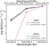 |
Fig. 1 Incident ionising flux -ϕ(H)) per energy and wavelength bin (CLOUDY model log U = −1.00, log n = 2, Z = 0.55 Z⊙) for SB99 (red lines) and BPASS (blue lines). The different SFH models are represented with solid (no quenching) and dashed lines (Δtզ = 5 Myr). |
2.3 Impact of SB99 versus BPASS on the HII region properties
As outlined in Sect. 2.2, in our work we computed the SED for three SFHs. The exponentially declining SFH and the continuous one return SEDs with comparable fluxes in all the energy bins (see Appendix A). For this reason, in the remainder of this work we only consider the continuous SFH and that characterised by the quenching episode 5 Myr prior to observation.
We started by analysing differences in the ionising-photon budget with a fixed SFH between SB99 and BPASS spectra. In Fig. 1 we show the incident H-ionising photon flux at the gas slab, ϕ, in bins with decreasing energy (A [272.1–54.4) eV, B [54.4–24.5) eV, and C [24.5–13.6) eV) for a fixed ionisation parameter, log U = −1, as computed by CLOUDY.
The impact binary stars have on the ionising photon budget is negligible for continuous SF (solid lines), and hence the SB99 and BPASS models are almost identical. In fact, stars are continuously formed and the youngest among them dominate the ionising photon flux in all the energy bins. The UV photons from binary systems are therefore negligible.
We instead observe differences if the SFH is characterised by a quenching episode. For SB99, the quenching of SF leads to a rapid decrease in ϕ in bins A and B (dotted and dashed red lines). This is not the case for BPASS, where the presence of binary stars keeps the EUV flux high, showing only some negligible differences in bin A (dotted and dashed blue lines). This behaviour is comparable to what has already been discussed in literature by Götberg et al. (2019) and presented for single starburst in Stanway & Eldridge (2018).
The different hardness of BPASS versus SB99 SEDs, for varying SFHs, affects the transition from the HII region to the PDR. This is shown in Fig. 2, where we plot the free-electron temperature (Te) and the H+ number density ( ) as a function of the gas column density for two CLOUDY models: log U = −4.00, log n = 3.00, Z = 0.55 Z⊙ (left panels), log U = −2.00, log n = 1.00, and Z = 0.55 Z⊙ (right panels). These are representative of typical ISM conditions inferred for ALPINE (see Table 3). The transition from the HII region to the PDR is marked by a drop in Te and
  .In the continuous SF case, the HII regions created by BPASS and SB99 approximately extend to comparable hydrogen column densities (NH ∼ 1019.2 cm−2 and NH ∼ 1020.8 cm−2 , respectively) and comparable temperature (T ∼ 104 K). The intensity of the ionising radiation determines the thickness of the HII region: an higher U results in a larger HII region. For the quenched SF cases, the BPASS SED keeps the HII region depth and temperature at values comparable to those produced by a continuous SF. On the other hand, the drop in the ionising photon budget for SB99 models causes the HII sizes to shrink, and their temperature to decrease. For larger U, the temperature drop is sharper, clearly separating the HII region from the PDR. Smaller U result in a smoother temperature drop, leading to a gradual transition from the HII region to the PDR. The same holds true for the
  profile. These differences, as we discuss later, affect the nebular emission from the ionised gas as well as the line ratios with respect to the [CII].
2.4 CLOUDY output
The CLOUDY outputs used in this work are the cumulative emergent fluxes (εline (n, U, Z) in erg s−1 cm−2) of selected emission lines as a function of NH . We used the εline at the end of the gas slab, where NH = 1022 cm−2. This is a conservative assumption because HII region tracers reach the plateau at NH ∼ 1019.2 cm−2 and NH ∼ 1020.8 cm−2 , respectively, for low U (left panels) and high U (right panels of Fig. 2). Out of all the possible lines, we focused on the emergent [CII] 158 µm flux as the ratios with respect to [CII] were later used to float our predictions for the nebular lines (Hβ, [OIII] 5007Å, Hα, [NII] 6583 Å). We also focused on the CIII]1909Å flux because theoretical studies (Feltre et al. 2016; Jaskot & Ravindranath 2016a; Nakajima et al. 2018) suggest that galaxies with low metallic- ities at z > 5 show prominent CIII] emission relative to other UV tracers. The current highest-redshift source spectroscopically confirmed with JWST (z = 14.32; Carniani et al. 2024) has a tentative CIII] 1907, 1909 Å doublet detection. Additionally, CIII] and [CII] emissions arise from the same element, so their ratio is unaffected by possible variations in the relative elemental abundances with Z. Through the paper we discuss in detail the CIII] 1909 Å, [OIII] 5007Å and Hα emission while the interested reader is referred to Appendix C for predictions concerning [NII] 6583 Å and Hβ.
In the upper panels of Fig. 3 we plot the [CII] cumulative flux, as a function of the hydrogen column density NH , for CLOUDY models corresponding to log U = −4.00, log n = 3.00, Z = 0.55 Z⊙ (left, low U), log U = −2.00, log n = 1.00, Z = 0.55 Z⊙ (right, high U), but characterised by different SFHs and/or stellar population. In general, all the models show a similar [CII] profile. However, in the high U case the [CII] cumulative flux produced by the SB99 quenched SF is systematically higher with respect to those produced by the other models. This is linked to the excitation energy of the transition (Tex ≈ 92 K; Osterbrock & Ferland 2006), making the [CII] emission only mildly sensitive to temperature variations in the PDR above ≈ 100 K. As can be noticed by looking at Fig. 2, the PDR plateau temperature of all the models is Te ∼ 100–200 K, but in the SB99 quenched SF case the PDR is more extended, thus boosting the [CII] emission.
In the middle panels of Fig. 3 we plot the cumulative flux of [OIII] as a function of NH for low U and high U. We observe a saturation of the cumulative flux of the line at NH ∼ 1019.2 cm−2 (left) and NH ∼ 1020.8 cm−2 (right), corresponding to the end of the HII region. This mirrors the temperature profile (see Fig. 2) that in the case of the SB99 quenched SFH drops at a slightly lower NH in both the low and high U cases. The [OIII] traces the ionised gas phase; thus an increasing U boosts the saturation plateau for all models. At fixed NH , we observe that in both low U and high U cases, the cumulative flux of [OIII] for SB99 quenched SF (dashed red lines) is systematically lower with respect to the other cases. This is due to the softer spectrum returned by SB99 for a quenched SF that reduces the thickness and temperature of the HII region (see Sect. 2.3). The [OIII] line is, indeed, extremely sensitive to temperature variations due to the high excitation energy (Tex > 20 000 K; Osterbrock & Ferland 2006). Even small Te variations in the HII region, caused by variations in U, SFH, and/or binary presence, have a significant impact on [OIII] emission. This is true for all the UV and optical lines that have a high excitation energy.
Finally, in the bottom panels of Fig. 3 we show the cumulative flux of Hα. At any fixed value of NH , the Hα cumulative flux in the SB99 quenched SF scenario (dashed red lines) is higher compared to the other cases. This depends on the SED normalisation with U. In fact, at fixed U the total number of photons above the Lyman limit (hν > 13.6 eV) is the same, but for the (softer) SED resulting from quenched SF this translates into an increase in the number of photons near 13 eV. This causes a slight enhancement in the Hα emission. Moreover, the temperature variation of the HII region minimally affects the Hα flux (emissivity ratio єHα/єHβ at fixed density log n = 2 cm−3 is 3.0, 2.8, and 2.7, respectively, at Tex = 5000, 10 000, and 20 000 K; Osterbrock & Ferland 2006).
In Fig. 4 we show the contour plots of the flux ratios between nebular lines and the [CII], as a function of n and U, assuming Z = 0.55 Z⊙. By comparing the observed nebular-to-[CII] line ratios with the theoretical contours, one can put constraints on the ISM properties characterising the targeted galaxies.
In the upper panels, we show the CIII]/[CII] ratio for BPASS continuous SF (left panel) and SB99 quenched SF (right panel). The ratio increases with increasing U and n. This is due to the rise of the cloud temperature/widening of the HII region with U (see Figs. 2 and 3), and to the higher CIII] critical density with respect to that of [CII]. SB99 quenched SF case shows, for fixed U and n, a systematically lower ratio with respect to the BPASS continuous SF case. This is due, as already discussed, to the softer spectrum returned by SB99 quenched SF case. In the middle panels, we show instead the [OIII]/[CII] ratio for BPASS continuous SF and SB99 quenched SF cases. This ratio shows a similar behaviour with respect to the CIII]/[CII] because of the same physical reasons. In the lower panels, we finally plot the Hα/[CII] ratio. As in the cases discussed above, the ratio increases with increasing n and U. However, the ratio remains the same between the BPASS continuous SF case and the SB99 quenched case for fixed U and n values. This trend can be explained by looking at Fig. 3. In both [CII] and Hα cases, the cumulative flux at NH = 1022 cm−2 increases in the SB99 quenched SF case, resulting in a ratio that remains the same as in the BPASS continuous SF case. The trends discussed so far are fundamental to interpreting the line luminosity predictions for ALPINE galaxies, which we discuss in Sect. 4.
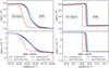 |
Fig. 2 Free electron temperature (Te; upper panels) and H+ number density ( |

Physical properties of the 44 ALPINE galaxies considered in this work.
3 Model application
3.1 Dataset
ALPINE (Béthermin et al. 2020; Le Fèvre et al. 2020; Faisst et al. 2020) is an ALMA large programme aimed at measuring [CII] 158 µm and rest-frame FIR continuum emission from a representative sample of 118 main-sequence galaxies at 4.4 < z < 5.8. Observations were carried out between May 2018 and February 2019 (Béthermin et al. 2020; Faisst et al. 2020). All galaxies are located in the Cosmic Evolution Survey (COSMOS; Scoville et al. 2007), and in the Extended Chandra Deep Field South (ECDFS; Giacconi et al. 2002) fields. The sample was selected to exclude as much as possible galaxies with evident active galactic nucleus signatures. However, a low-luminosity active galactic nucleus was recently discovered in one source of the sample (GDS J033218.92-275302.7; Barchiesi et al. 2023; Übler et al. 2023). ALPINE galaxies are characterised by SFR≳ 10 M⊙ yr−1 and stellar masses M⋆ ~ 109–1011 M⊙ (Faisst et al. 2020). Among the 118 sources, 75 and 23 are [CII] and 158 µm continuum detected, respectively.
For the present analysis, we selected a subset of 44 galaxies with measured [CII] luminosities (Faisst et al. 2020) and UV radii (Fujimoto et al. 2020). These galaxies represent the complete subsample of Fujimoto et al. (2020), excluding two galaxies lacking in SFR and UV radius data (Table 3). The UV radius data, together with the SFR, are needed to exploit the analytical model described in Sect. 3.2 used to infer the fiducial n and U values for the ALPINE galaxies. In our work we considered the total SFR (SFRUV+IR), namely the sum of the unobscured (SFRUV) and obscured (SFRIR) one. We derived the SFRUV from the UV luminosity at 1500 Å (Faisst et al. 2020) uncorrected for dust extinction and the SFRIR from the IR luminosity reported in (Béthermin et al. 2020) using the Kennicutt (1998) relation. For the galaxies not detected in continuum with ALMA, we derived the LIR from the infrared excess (LIR/LUV) computed for the ALPINE galaxies by Fudamoto et al. (2020) from the UV spectral slope, β.
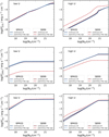 |
Fig. 3 Cumulative flux of [CII] 158 µm (upper panels), [OIII]5007 Å (middle panels), and Hα (lower panels) as a function of the hydrogen column density (NH). We show CLOUDY models log U = −4.00, log n = 3.00, Z = 0.5 5 Z⊙ (left panel; low U) and log U = −2.00, log n = 1.00, Z = 0.55 Z⊙ (right panel; high U). The different SFHs are represented with solid (continuous SF) and dashed lines (quenching Δtq = 5 Myr). Red lines are associated with SB99 models, blue with BPASS models. |
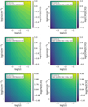 |
Fig. 4 Contour plots of the ratio between the [CII] line and the cumulative flux of CIII]1909 Å (upper panels), [OIII]5007 Å (middle panels), and Hα (lower panels) as a function of the ionisation parameter (U) and the H number density (n). The gas metallicity is fixed to Z = 0.55 Z⊙. Left panels: CLOUDY models using BPASS with a continuous SFH. Right panels: CLOUDY models using SB99 with a quenched SFH (Δtq = 5 Myr). |
3.2 Fiducial CLOUDY models for ALPINE
Following Ferrara et al. (2019) (F19 hereafter), we assumed that each galaxy can be represented as a flat, parallel slab of gas with a uniform number density (n), metallicity (Z), and total gas column density (Σgas). The slab is illuminated by a (stellar) source of ionising and non-ionising radiation. F19 allowed us to infer (n, U) – two of the three free parameters of the CLOUDY models (see Sect. 2.1) – by linking them to global galaxy properties using the following relations:
![Mathematical equation: $n = 5.4 \times {10^{ - 13}}{\Sigma _{{\rm{gas}}}}^2{\sigma ^{ - 2}}\left[ {{\rm{c}}{{\rm{m}}^{ - 3}}} \right],$](/articles/aa/full_html/2025/01/aa51111-24/aa51111-24-eq10.png) (3)
(3)
 (4)
(4)
where ∑gas is the gas surface density, ∑SFR is the SFR surface density, and σ is the rms turbulent velocity in km/s. We derived the ΣSFR from the SFRUV+IR and the IR radius (rIR) for the ALPINE galaxies. Given the recent results by Pozzi et al. (2024) in ALPINE and Mitsuhashi et al. (2024) in CRISTAL, we assumed rIR = 2rUV. We assumed σ ≈ 50 km s−1, the average value found for the ALPINE sample by Jones et al. (2021) and Parlanti et al. (2023) based on low-resolution observations. This value approaches the upper limits measured in high-resolution studies of starburst galaxies (σ ≈ 40 km s−1 ; Rizzo et al. 2021; Lelli et al. 2021; Roman-Oliveira et al. 2023). Choosing a reasonable σ is crucial due to its impact in estimating the gas density, n. Halving σ quadruples the value of n, as shown in Eq. (3).
We instead computed the Σgas using the Kennicutt-Schmidt (KS) relation (Heiderman et al. 2010), adopting the notation introduced by F19:
![Mathematical equation: ${\Sigma _{{\rm{SFR}}}} = {10^{ - 12}}{k_s}\Sigma _{{\rm{gas}}}^m\left[ {{{\rm{M}}_ \odot }{\rm{y}}{{\rm{r}}^{ - 1}}{\rm{kp}}{{\rm{c}}^{ - 2}}} \right]\quad ({\rm{m}} = 1.4).$](/articles/aa/full_html/2025/01/aa51111-24/aa51111-24-eq12.png) (5)
(5)
In Eq. (5), F19 defined the burstiness parameter (ks), defined as the deviation from the KS relation. Galaxies with ks > 1 have a larger SFR per unit area with respect to those located on the KS relation, so they are starburst and can convert gas in stars more efficiently with a shorter depletion time (tdep).
Equation (5) ultimately allows us to derive Σgas from the measured ∑SFR in ALPINE as a function of the free parameter ks. We assumed four different values for the ks parameters. From the spatially resolved analysis presented by Béthermin et al. (2023) for four ALPINE galaxies the average value of the burstiness parameter is 0.34 (see Fig. 5) derived by converting the depletion time  . Moreover, we also considered ks = 5 and ks = 10, which are values representative of moderate and extreme starburst galaxies at high z (Vallini et al. 2021), and the ‘standard’ KS law, namely ks = 1. The galaxies presented in Béthermin et al. (2023) are among the brightest [CII] galaxies in the ALPINE sample. This is why, in order to avoid bias, we included predictions for various ks values. For ks = 0.34, using Eqs. (3), (4), and (5), we obtain a median value log U = −3.8 ± 0.2 and log(n/cm−3) = 2.9 ± 0.6 within our ALPINE subsample. The associated errors are the subsample standard deviations for the two parameters. These are comparable with those inferred by Vanderhoof et al. (2022) for ten ALPINE galaxies, where the measured dust-corrected luminosity ratios of log(L[OII] /L[CII]) and log(L[OII] /LHα) required ionisation parameters log(U) < −2 and electron densities log(ne/[cm−3]) ≈ 2.5–3. In Table 3 we report the ALPINE fiducial U and n values and those computed for ks = 1, 5, 10.
The inferred n and U for each ALPINE galaxy were then exploited to compute
![Mathematical equation: $L_{line{\rm{ }}}^{pred{\rm{ }}} = {R_{line{\rm{ }}}}(n,U,Z) \times L_{[{\rm{CII}}]}^{obs}$](/articles/aa/full_html/2025/01/aa51111-24/aa51111-24-eq14.png) (6)
(6)
from the corresponding CLOUDY models, where
![Mathematical equation: ${R_{line{\rm{ }}}}(n,U,Z) = {{{\varepsilon _{line{\rm{ }}}}(n,U,Z)} \over {{\varepsilon _{{\rm{[CII]}}}}(n,U,Z)}}$](/articles/aa/full_html/2025/01/aa51111-24/aa51111-24-eq15.png) (7)
(7)
is the CLOUDY predicted ratio of each line with respect to the [CII]. For the entire ALPINE sample we assumed Z = 0.5 Z⊙, similar to what has been found in Vanderhoof et al. (2022) from UV absorption lines in ALPINE sample. The gas metallicity has a smaller impact on the line ratios with respect to n and U. For fixed values of n and U, the line ratio increases of 0.34 – 40.4 dex when metallicity varies from 0.15 Z⊙ to 0.55 Z⊙. However, we defer a dedicated analysis to a future work.
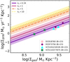 |
Fig. 5 KS law (solid magenta line; Heiderman et al. 2010). The coloured points represent the location on the KS plane of the subset of ALPINE galaxies analysed by Béthermin et al. (2023). Each galaxy is resolved in two different beams, providing two measures for Σgas and ∑SFR. Following the notation of Ferrara et al. (2019), this corresponds to a burstiness parameter ks = 0.34 (purple line). For comparison, we also report the relation obtained by substituting ks = 5 and 10 in Eq. (5) with dashed orange and dotted yellow lines, respectively. The y dispersion is σ = 0.28. |
4 Results
Nebular line predictions and their relation with the SFR
Following the procedure described in Sect. 3, for each ALPINE galaxy we derived theoretical predictions for the nebular line luminosities starting from Rline(n, U, Z) and the observed L[CII]. We then derived relations between the theoretical line luminosity and the total observed SFRUV+IR ,
 (8)
(8)
by employing a Bayesian Markov chain Monte Carlo fitting method implemented with the open-source Python package emcee (Foreman-Mackey et al. 2013). We ran emcee with 44 random walkers exploring the parameter space for 5 × 10³ chain steps. Table 4 summarises the slope (α) and intercept (β) coefficients for the BPASS cases together with their 1σ dispersion for the fiducial ALPINE model (ks = 0.34) and for ks = 1, 5, and 102.
In Fig. 6 (left panel) we show the best-fit LCIII]–SFRUV+IR relations, together with their 1–2σ dispersion, for the two considered SFHs and assuming ks = 0.34. Figure 6 highlights the strong impact of considering binary stars when computing the radiation illuminating the ISM. For models without binaries (SB99 cases), the CIII] is sensitive to SF quenching. In the SB99 quenched SF case (upper panel), the CIII] emission drops by almost 1 dex at a fixed SFR for Δtq = 5 Myr. This is a consequence of the very high ionising potential of C+ (24.45 eV) and the shrinking of the HII region due to a softer incident spectrum (see Sects. 2.3 and 2.4). BPASS models (lower panel), on the other hand, are not influenced by quenching since the emission remains stable up to Δtq = 5 Myr. This is due to binaries being able to delay the drop of the UV photon budget for a stellar population that is experiencing a quenching in SF.
In Fig. 6 (right panel) we show the best-fit LCIII]-SFRUV+IR relations, together with their 1–2σ dispersion assuming ks = 5. The observed trends are comparable to those shown for ks = 0.34. The relations obtained for ks = 5 agree within the errors with the location onto the LCIII]-SFRUV+IR plane of z ≈ 3 low- mass star-forming galaxies with stellar masses in the range 7.9 < log(M⋆/M⊙) < 10.3 selected from the CIII] 1909 Å emission by Llerena et al. (2023). This is true for all SFH scenarios examined in this work for BPASS, as well as in the case of a continuous SF assuming a SB99 spectrum. In Fig. 6 we also include the z ≈ 6–7 sources from Markov et al. (2022), jointly detected in CIII] 1909 Å and [CII] 158µm. Markov et al. (2022) data are systematically higher than our best-fit relations. This suggests that the three galaxies are experiencing starburst phase (ks > 5, in line with the conclusions by Markov et al. 2022).
With a fixed SFR, the CIII] luminosity for ks = 5 is systematically higher than that obtained for ks = 0.34. Using ks = 0.34 results in higher values of gas surface densities compared to ks = 5 (see Eq. (5)). This results in a relatively high cloud density n and a relatively low ionisation parameter for ks = 0.34 compared to ks = 5 (see Eq. (3)). A small value of U will produce a small HII region (see Fig. 2), thus reducing the emission of UV and optical lines with high ionisation energies, as already remarked in Sect. 2.4.
In Fig. 7 we show the theoretical predictions for the [OIII] 5007 Å line for ks = 0.34 (left panel) and ks = 5 (right panel). The data presented by Llerena et al. (2023) are near the best-fit relation found with ks = 5, in the two SFH scenarios examined in the BPASS case, as well as in the case of a continuous SF for SB99. As for CIII], binary systems keep the brightness of the [OIII] line constant even if the galaxy is experiencing a quenching of Δtq = 5 Myr. SB99 quenched SF cases show instead a large drop in L[OIII] , as already underlined for CIII]. This is related to the ionisation potential of O+ (35.1 eV) and to the shrinking of HII region due to a softer incident spectrum.
In Fig. 8 we show the predictions for the Hα line. Contrary to CIII] and [OIII] 5007Å (Figs. 6 and 7) the Hα line does not show a marked dependence on the presence of a quenching in SF, at least up to Δtq = 5 Myr, in both the BPASS and SB99 cases. This is due to the behaviour of the cumulative flux of [CII] and Hα in the case of quenching discussed in Sect. 2.4. For SB99, both lines show an enhancement in flux for the quenched case. The result is that the ratio between the two lines does not vary. For BPASS, due to the presence of binaries (see Sect. 2.3), the emission of the two lines is not affected by the quenching in SF, so the ratio remains constant.
Hα predictions represent a key tool for verifying whether our model can reproduce well-established relationships from the literature that link Hα to the SFR of a galaxy (e.g. Kennicutt 1998; Kennicutt & Evans 2012). As outlined in Fig. 8, our model is able to reproduce these relationships, within a factor of 10. For ks = 0.34 (left panel), we observe that the Kennicutt (1998) and Kennicutt & Evans (2012) relations agree within 1–2σ dispersion of our modelling fits. For ks = 5 (right panel) the predictions consistently exceed those from Kennicutt (1998); Kennicutt & Evans (2012), even remaining in the region of 2σ dispersion. These results suggest that caution should be taken when applying locally calibrated relations to starburst galaxies. The Hα predictions are not significantly affected by an abrupt quenching Δtq = 5 Myr or by the presence of binary systems. This aligns with the fact that 90% of the Hα emission originates from a stellar population with an average age of 10 Myr, precluding observable luminosity variations in the analysed quenching scenario (Kennicutt & Evans 2012).
Considering the BPASS models as fiducial given the inclusion of binary stars, the UV and optical lines are not affected by the SFH of a galaxy. Instead, the line luminosity depends on the assumed value of the ks parameter (see Table 4). From the position of an observed galaxy in the UV/optical-SFR relations, we can therefore place a constraint on the galaxy’s deviation from the local KS relation (i.e. an estimation for the ks parameter), for instance the constraint already proposed in Vallini et al. (2021, 2024) for FIR lines (for Hβ and [NII] predictions, see Appendix C).
Slope (α) and intercept (β) of the linear regression for the CIII] 1909 Å, [OIII] 5007 Å, and Hα lines.
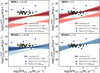 |
Fig. 6 Predicted luminosity of CIII] 1909 Å as a function of the total SFR (SFRUV+IR) for ks = 0.34 (left panel) and ks = 5 (right panel). The colours correspond to 1–2σ dispersion. The central region between the dashed grey lines represents the SFR range of the ALPINE subsample modelled in this work. Red and blue represent the two SFHs considered in this work: continuous and Δtq = 5 Myr. The black points are the observed data from Llerena et al. (2023), the blue points from Markov et al. (2022). |
5 Conclusions
In this work we have developed a physically motivated ISM model for the line emission from HII regions and PDRs using CLOUDY (Ferland et al. 2017) and two different codes for simulating the incident radiation from a stellar population: SB99 and BPASS (the latter includes binary stars). By using the theoretical ratio from our model, we obtained predictions for the UV/optical line luminosity from the observed [CII] luminosity for a subsample of ALPINE galaxies. The main results can be summarised as follows:
The presence of binary stars as modelled by the BPASS code makes the UV spectrum from a composite stellar population harder with respect to what is obtained with SB99 without binary systems. This effect is particularly evident for a quenched SFH as binary stars delay the drop in the EUV photon flux after the quenching. The EUV flux is sustained by UV photon production from mass-exchange processes in binary systems. These processes significantly affect the ionising photon rate and hence the size and temperature of the HII regions. Assuming an abrupt SF quenching for SB99 models, the decrease in the EUV photon budget in the incident radiation reduces the width and alters the chemical properties of the HII region. Conversely, the binary stars included in the BPASS code are able to sustain emission in EUV after quenching, thus keeping the HII region unchanged for at least Δtq = 5 Myr. Therefore, the presence of binaries must be considered in a complete line emission model (as suggested by e.g. Jaskot & Ravindranath 2016a);
We derived the ISM physical properties (hydrogen density, n, and ionisation parameter, U) of a subsample of 44 ALPINE galaxies. We used the analytical model from Ferrara et al. (2019) to associate n and U with the gas surface density (Σgas), obtained from the KS relation, and the SF surface density (ΣSFR) of each galaxy, through the burstiness parameter, ks . For the ALPINE subsample we considered a fiducial value of ks = 0.34, estimated from Béthermin et al. (2023) data. We obtain log U0.34 (−3.8 ± 0.2) and log n0.34 (2.9 ± 0.6). These values are consistent with those inferred by Vanderhoof et al. (2022), who investigated a smaller subset of ALPINE galaxies;
We derived UV/optical lines luminosities-SFR relations in the form log(Lline/ergs−1) = α log(SFR/M⊙ yr−1) + β for different ks values: the fiducial for ALPINE galaxies (ks ≈ 0.34) and ks = 1, 5, and 10 (see Table 4). We suggest that these relations, which are in line with the high-z data from Llerena et al. (2023), can be used at high z for galaxy SFR characterisation. The strong alignment of the Kennicutt (1998) and Kennicutt & Evans (2012) relations with our model predictions for ks = 0.34 attests to our models’ robustness. For starburst galaxies (ks > 1), our predictions exceed those of the Kennicutt relation, suggesting caution should be taken when applying locally calibrated Kennicutt laws to highly efficient star-forming galaxies;
In the models that use the spectral synthesis code BPASS to estimate the radiation from the stellar population, the relations have a negligible SFH dependence but a strong dependence on the ks value, with line luminosities increasing for higher ks (i.e. for starburst galaxies). For the SB99 cases, the key dependence is on the SFH, and the lack of binaries results in a significant flux drop even after a short quenching period (Δtq = 5 Myr) for at least a UV/optical line with a high ionisation energy.
Our method can be used to place stringent constraints on the UV/optical line luminosities, drawing from the robust [CII] ALMA observations. Looking ahead, the future JWST follow-up of ALMA observations promises to provide state-of-the-art data that can be used to test the efficacy of our method in characterising the SFR of high-z galaxies, and to allow us to characterise the SF mode in galaxies at the end of the EoR. In a forthcoming paper, the imminent JWST NIRSpec integral field unit observations of 18 ALPINE galaxies will offer a great opportunity to exploit our theoretical predictions, thereby potentially confirming the physical properties found for these galaxies.
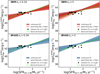 |
Fig. 8 Same as Fig. 6 but for Hα 6563 Å. The dashed green line is the Kennicutt & Evans (2012) relation. |
Acknowledgements
We thank the anonymous referee for their constructive report, which helped to improve the quality of this work. MB gratefully acknowledges support from the ANID BASAL project FB210003 and from the FONDECYT regular grant 1211000. This work was supported by the French government through the France 2030 investment plan managed by the National Research Agency (ANR), as part of the Initiative of Excellence of Univer- sité Côte d’Azur under reference number ANR-15-IDEX-01. MR acknowledges support from the Narodowe Centrum Nauki (UMO-2020/38/E/ST9/00077) and support from the Foundation for Polish Science (FNP) under the program START 063.2023. EI acknowledge funding by ANID FONDECYT Regular 1221846. FE acknowledges support from grant PRIN MIUR 2017-20173ML3WW_001. LV, FE acknowledge funding from the INAF Mini Grant 2022 program “Face-to- Face with the Local Universe: ISM Empowerment (LOCAL)”.
Appendix A Exponential declining SF
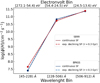 |
Fig. A.1 Incident ionising flux, ϕ(H), per energy bin and wavelength bin (CLOUDY models U = −1.00, n = 2, Z = 0.55 Z⊙) for BPASS (blue lines) and SB99 (red lines). The different SFH models are represented with solid (continuous SF) and dashed lines (exponential declining SF τ = 0.3 Gyr). |
Appendix B CIII], [OIII], and Hα SB99 predictions
Slope (α) and intercept (β) of the linear regression for the CIII] 1909A˚, [OIII] 5007Å, and Hα lines.
Appendix C [NII] and Hβ predictions
Slope (α) and intercept (β) of the linear regression for the [NII]6583Å and Hβ lines.
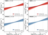 |
Fig. C.2 Same as Fig. 6 but for Hβ. |
References
- Arata, S., Yajima, H., Nagamine, K., Abe, M., & Khochfar, S. 2020, MNRAS, 498, 5541 [NASA ADS] [CrossRef] [Google Scholar]
- Backhaus, B. E., Trump, J. R., Pirzkal, N., et al. 2024, ApJ, 962, 195 [NASA ADS] [CrossRef] [Google Scholar]
- Baldwin, J. A., Ferland, G. J., Martin, P. G., et al. 1991, ApJ, 374, 580 [Google Scholar]
- Barchiesi, L., Dessauges-Zavadsky, M., Vignali, C., et al. 2023, A&A, 675, A30 [NASA ADS] [CrossRef] [EDP Sciences] [Google Scholar]
- Behrens, C., Pallottini, A., Ferrara, A., Gallerani, S., & Vallini, L. 2018, MNRAS, 477, 552 [NASA ADS] [CrossRef] [Google Scholar]
- Béthermin, M., Fudamoto, Y., Ginolfi, M., et al. 2020, A&A, 643, A2 [Google Scholar]
- Béthermin, M., Accard, C., Guillaume, C., et al. 2023, A&A, 680, L8 [NASA ADS] [CrossRef] [EDP Sciences] [Google Scholar]
- Bouwens, R. J., Smit, R., Schouws, S., et al. 2022, ApJ, 931, 160 [NASA ADS] [CrossRef] [Google Scholar]
- Bunker, A. J., Saxena, A., Cameron, A. J., et al. 2023, A&A, 677, A88 [NASA ADS] [CrossRef] [EDP Sciences] [Google Scholar]
- Carilli, C. L., & Walter, F. 2013, ARA&A, 51, 105 [NASA ADS] [CrossRef] [Google Scholar]
- Carniani, S., Maiolino, R., Smit, R., & Amorín, R. 2018, ApJ, 854, L7 [Google Scholar]
- Carniani, S., Hainline, K., D’Eugenio, F., et al. 2024, Nature, 633, 318 [CrossRef] [Google Scholar]
- Chabrier, G. 2003, PASP, 115, 763 [Google Scholar]
- Chatzikos, M., Bianchi, S., Camilloni, F., et al. 2023, Rev. Mexicana Astron. Astrofis., 59, 327 [Google Scholar]
- Curti, M., D’Eugenio, F., Carniani, S., et al. 2023, MNRAS, 518, 425 [Google Scholar]
- Dayal, P., & Ferrara, A. 2018, Phys. Rep., 780, 1 [Google Scholar]
- De Looze, I., Cormier, D., Lebouteiller, V., et al. 2014, A&A, 568, A62 [NASA ADS] [CrossRef] [EDP Sciences] [Google Scholar]
- Dessauges-Zavadsky, M., Ginolfi, M., Pozzi, F., et al. 2020, A&A, 643, A5 [NASA ADS] [CrossRef] [EDP Sciences] [Google Scholar]
- Di Cesare, C., Graziani, L., Schneider, R., et al. 2023, MNRAS, 519, 4632 [Google Scholar]
- Donnan, C. T., McLure, R. J., Dunlop, J. S., et al. 2024, MNRAS, 533, 3222 [NASA ADS] [CrossRef] [Google Scholar]
- Dunlop, J. S., Abraham, R. G., Ashby, M. L. N., et al. 2021, PRIMER: Public Release IMaging for Extragalactic Research, JWST Proposal. Cycle 1, 1837 [Google Scholar]
- Eisenstein, D. J., Willott, C., Alberts, S., et al. 2023, ApJS, Submitted [arXiv:2306.02465] [Google Scholar]
- Eldridge, J. J., & Stanway, E. R. 2022, ARA&A, 60, 455 [NASA ADS] [CrossRef] [Google Scholar]
- Faisst, A. L., Capak, P. L., Davidzon, I., et al. 2016, ApJ, 822, 29 [Google Scholar]
- Faisst, A. L., Schaerer, D., Lemaux, B. C., et al. 2020, ApJS, 247, 61 [NASA ADS] [CrossRef] [Google Scholar]
- Feltre, A., Charlot, S., & Gutkin, J. 2016, MNRAS, 456, 3354 [Google Scholar]
- Ferland, G. J., Chatzikos, M., Guzmán, F., et al. 2017, Rev. Mexicana Astron. Astrofis., 53, 385 [Google Scholar]
- Ferrara, A., Vallini, L., Pallottini, A., et al. 2019, MNRAS, 489, 1 [Google Scholar]
- Foreman-Mackey, D., Hogg, D. W., Lang, D., & Goodman, J. 2013, PASP, 125, 306 [Google Scholar]
- Fudamoto, Y., Oesch, P. A., Faisst, A., et al. 2020, A&A, 643, A4 [NASA ADS] [CrossRef] [EDP Sciences] [Google Scholar]
- Fujimoto, S., Silverman, J. D., Bethermin, M., et al. 2020, ApJ, 900, 1 [Google Scholar]
- Giacconi, R., Zirm, A., Wang, J., et al. 2002, ApJS, 139, 369 [Google Scholar]
- Grevesse, N., Asplund, M., Sauval, A. J., & Scott, P. 2010, Ap&SS, 328, 179 [Google Scholar]
- Götberg, Y., de Mink, S. E., Groh, J. H., Leitherer, C., & Norman, C. 2019, A&A, 629, A134 [NASA ADS] [CrossRef] [EDP Sciences] [Google Scholar]
- Heiderman, A., Evans I., Neal J., Allen, L. E., Huard, T., & Heyer, M. 2010, ApJ, 723, 1019 [NASA ADS] [CrossRef] [Google Scholar]
- Indriolo, N., Geballe, T. R., Oka, T., & McCall, B. J. 2007, ApJ, 671, 1736 [NASA ADS] [CrossRef] [Google Scholar]
- Isobe, Y., Ouchi, M., Nakajima, K., et al. 2023, ApJ, 956, 139 [NASA ADS] [CrossRef] [Google Scholar]
- Jaskot, A. E., & Ravindranath, S. 2016a, ApJ, 833, 136 [NASA ADS] [CrossRef] [Google Scholar]
- Jones, G. C., Vergani, D., Romano, M., et al. 2021, MNRAS, 507, 3540 [NASA ADS] [CrossRef] [Google Scholar]
- Karttunen. 2007, Fundamental Astronomy (Springer) [CrossRef] [Google Scholar]
- Katz, H., Kimm, T., Sijacki, D., & Haehnelt, M. G. 2017, MNRAS, 468, 4831 [Google Scholar]
- Katz, H., Rosdahl, J., Kimm, T., et al. 2022, MNRAS, 510, 5603 [NASA ADS] [CrossRef] [Google Scholar]
- Kennicutt J., Robert C., 1998, ARA&A, 36, 189 [NASA ADS] [CrossRef] [Google Scholar]
- Kennicutt, R. C., & Evans, N. J. 2012, ARA&A, 50, 531 [NASA ADS] [CrossRef] [Google Scholar]
- Kewley, L. J., Nicholls, D. C., & Sutherland, R. S. 2019, ARA&A, 57, 511 [Google Scholar]
- Kohandel, M., Pallottini, A., Ferrara, A., et al. 2020, MNRAS, 499, 1250 [Google Scholar]
- Kriek, M., Shapley, A. E., Reddy, N. A., et al. 2015, ApJS, 218, 15 [NASA ADS] [CrossRef] [Google Scholar]
- Lagache, G., Cousin, M., & Chatzikos, M. 2018, A&A, 609, A130 [NASA ADS] [CrossRef] [EDP Sciences] [Google Scholar]
- Le Fèvre, O., Béthermin, M., Faisst, A., et al. 2020, A&A, 643, A1 [Google Scholar]
- Leitherer, C., Schaerer, D., Goldader, J. D., et al. 1999, ApJS, 123, 3 [Google Scholar]
- Lelli, F., Di Teodoro, E. M., Fraternali, F., et al. 2021, Science, 371, 713 [Google Scholar]
- Llerena, M., Amorín, R., Pentericci, L., et al. 2023, A&A, 676, A53 [NASA ADS] [CrossRef] [EDP Sciences] [Google Scholar]
- Lupi, A., Pallottini, A., Ferrara, A., et al. 2020, MNRAS, 496, 5160 [Google Scholar]
- Maiolino, R., Carniani, S., Fontana, A., et al. 2015, MNRAS, 452, 54 [NASA ADS] [CrossRef] [Google Scholar]
- Markov, V., Carniani, S., Vallini, L., et al. 2022, A&A, 663, A172 [NASA ADS] [CrossRef] [EDP Sciences] [Google Scholar]
- Mather, J. C., Fixsen, D. J., Shafer, R. A., Mosier, C., & Wilkinson, D. T. 1999, ApJ, 512, 511 [Google Scholar]
- Mathis, J. S., Rumpl, W., & Nordsieck, K. H. 1977, ApJ, 217, 425 [Google Scholar]
- Matthee, J., Sobral, D., Boogaard, L. A., et al. 2019, ApJ, 881, 124 [NASA ADS] [CrossRef] [Google Scholar]
- McLure, R. J., Pentericci, L., Cimatti, A., et al. 2018, MNRAS, 479, 25 [NASA ADS] [Google Scholar]
- Mitsuhashi, I., Tadaki, K.-i., Ikeda, R., et al. 2024, A&A, 690, A197 [NASA ADS] [CrossRef] [EDP Sciences] [Google Scholar]
- Moriwaki, K., Yoshida, N., Shimizu, I., et al. 2018, MNRAS, 481, L84 [NASA ADS] [CrossRef] [Google Scholar]
- Nakajima, K., Schaerer, D., Le Fèvre, O., et al. 2018, A&A, 612, A94 [NASA ADS] [CrossRef] [EDP Sciences] [Google Scholar]
- Nakazato, Y., Yoshida, N., & Ceverino, D. 2023, ApJ, 953, 140 [NASA ADS] [CrossRef] [Google Scholar]
- Osterbrock, D. E., & Ferland, G. J. 2006, Astrophysics of Gaseous Nebulae and Active Galactic Nuclei (University Science Books) [Google Scholar]
- Pallottini, A., Ferrara, A., Decataldo, D., et al. 2019, MNRAS, 487, 1689 [Google Scholar]
- Pallottini, A., Ferrara, A., Gallerani, S., et al. 2022, MNRAS, 513, 5621 [NASA ADS] [Google Scholar]
- Parlanti, E., Carniani, S., Pallottini, A., et al. 2023, A&A, 673, A153 [NASA ADS] [CrossRef] [EDP Sciences] [Google Scholar]
- Pozzi, F., Calura, F., Fudamoto, Y., et al. 2021, A&A, 653, A84 [NASA ADS] [CrossRef] [EDP Sciences] [Google Scholar]
- Pozzi, F., Calura, F., D’Amato, Q., et al. 2024, A&A, 686, A187 [NASA ADS] [CrossRef] [EDP Sciences] [Google Scholar]
- Rieke, M. J., Robertson, B., Tacchella, S., et al. 2023, ApJS, 269, 16 [NASA ADS] [CrossRef] [Google Scholar]
- Rizzo, F., Vegetti, S., Fraternali, F., Stacey, H. R., & Powell, D. 2021, MNRAS, 507, 3952 [NASA ADS] [CrossRef] [Google Scholar]
- Robertson, B. E. 2022, ARA&A, 60, 121 [NASA ADS] [CrossRef] [Google Scholar]
- Roman-Oliveira, F., Fraternali, F., & Rizzo, F. 2023, MNRAS, 521, 1045 [NASA ADS] [CrossRef] [Google Scholar]
- Romano, M., Morselli, L., Cassata, P., et al. 2022, A&A, 660, A14 [NASA ADS] [CrossRef] [EDP Sciences] [Google Scholar]
- Schaerer, D., Meynet, G., Maeder, A., & Schaller, G. 1993, A&AS, 98, 523 [NASA ADS] [Google Scholar]
- Schaerer, D., Ginolfi, M., Béthermin, M., et al. 2020, A&A, 643, A3 [NASA ADS] [CrossRef] [EDP Sciences] [Google Scholar]
- Schaerer, D., Marques-Chaves, R., Barrufet, L., et al. 2022, A&A, 665, L4 [NASA ADS] [CrossRef] [EDP Sciences] [Google Scholar]
- Scoville, N., Aussel, H., Brusa, M., et al. 2007, ApJS, 172, 1 [Google Scholar]
- Sommovigo, L., Ferrara, A., Carniani, S., et al. 2021, MNRAS, 503, 4878 [NASA ADS] [CrossRef] [Google Scholar]
- Stacey, G. J., Hailey-Dunsheath, S., Ferkinhoff, C., et al. 2010, ApJ, 724, 957 [NASA ADS] [CrossRef] [Google Scholar]
- Stanway, E. R., & Eldridge, J. J. 2018, MNRAS, 479, 75 [NASA ADS] [CrossRef] [Google Scholar]
- Stanway, E. R., Eldridge, J. J., Greis, S. M. L., et al. 2014, MNRAS, 444, 3466 [Google Scholar]
- Steidel, C. 2014, KBSS-MOSFIRE: Deep Near-IR Spectroscopy of High-z Galaxies in the Keck Baryonic Structure Survey Fields, Keck Observatory Archive MOSFIRE, C223M [Google Scholar]
- Tacchella, S., Johnson, B. D., Robertson, B. E., et al. 2023, MNRAS, 522, 6236 [NASA ADS] [CrossRef] [Google Scholar]
- Tacconi, L. J., Genzel, R., & Sternberg, A. 2020, ARA&A, 58, 157 [NASA ADS] [CrossRef] [Google Scholar]
- Übler, H., Maiolino, R., Curtis-Lake, E., et al. 2023, A&A, 677, A145 [NASA ADS] [CrossRef] [EDP Sciences] [Google Scholar]
- Vallini, L., Gallerani, S., Ferrara, A., Pallottini, A., & Yue, B. 2015, ApJ, 813, 36 [NASA ADS] [CrossRef] [Google Scholar]
- Vallini, L., Ferrara, A., Pallottini, A., Carniani, S., & Gallerani, S. 2021, MNRAS, 505, 5543 [NASA ADS] [CrossRef] [Google Scholar]
- Vallini, L., Witstok, J., Sommovigo, L., et al. 2024, MNRAS, 527, 10 [Google Scholar]
- Vanderhoof, B. N., Faisst, A. L., Shen, L., et al. 2022, MNRAS, 511, 1303 [NASA ADS] [CrossRef] [Google Scholar]
- van Hoof, P. A. M., Weingartner, J. C., Martin, P. G., Volk, K., & Ferland, G. J. 2004, MNRAS, 350, 1330 [NASA ADS] [CrossRef] [Google Scholar]
- Venturi, G., Carniani, S., Parlanti, E., et al. 2024, A&A, 691, A19 [NASA ADS] [CrossRef] [EDP Sciences] [Google Scholar]
- Weingartner, J. C., & Draine, B. T. 2001, ApJ, 563, 842 [NASA ADS] [CrossRef] [Google Scholar]
- Weingartner, J. C., Draine, B. T., & Barr, D. K. 2006, ApJ, 645, 1188 [NASA ADS] [CrossRef] [Google Scholar]
- Wolfire, M. G., Vallini, L., & Chevance, M. 2022, ARA&A, 60, 247 [NASA ADS] [CrossRef] [Google Scholar]
- Xiao, L., Stanway, E. R., & Eldridge, J. J. 2018, MNRAS, 477, 904 [Google Scholar]
- Xiao, L., Galbany, L., Eldridge, J. J., & Stanway, E. R. 2019, MNRAS, 482, 384 [NASA ADS] [CrossRef] [Google Scholar]
- Yang, G., Caputi, K. I., Papovich, C., et al. 2023, ApJ, 950, L5 [NASA ADS] [CrossRef] [Google Scholar]
- Zanella, A., Daddi, E., Magdis, G., et al. 2018, MNRAS, 481, 1976 [Google Scholar]
The ionisation parameter (U) is defined as the dimensionless ratio of hydrogen-ionising photon flux (ϕ) to total-hydrogen density (n) at the illuminated face of the gas slab:
 (1)
(1)
The SB99 cases are reported in Appendix B.
All Tables
Slope (α) and intercept (β) of the linear regression for the CIII] 1909 Å, [OIII] 5007 Å, and Hα lines.
Slope (α) and intercept (β) of the linear regression for the CIII] 1909A˚, [OIII] 5007Å, and Hα lines.
Slope (α) and intercept (β) of the linear regression for the [NII]6583Å and Hβ lines.
All Figures
|
Fig. 1 Incident ionising flux -ϕ(H)) per energy and wavelength bin (CLOUDY model log U = −1.00, log n = 2, Z = 0.55 Z⊙) for SB99 (red lines) and BPASS (blue lines). The different SFH models are represented with solid (no quenching) and dashed lines (Δtզ = 5 Myr). |
| In the text | |
|
Fig. 2 Free electron temperature (Te; upper panels) and H+ number density ( |
| In the text | |
|
Fig. 3 Cumulative flux of [CII] 158 µm (upper panels), [OIII]5007 Å (middle panels), and Hα (lower panels) as a function of the hydrogen column density (NH). We show CLOUDY models log U = −4.00, log n = 3.00, Z = 0.5 5 Z⊙ (left panel; low U) and log U = −2.00, log n = 1.00, Z = 0.55 Z⊙ (right panel; high U). The different SFHs are represented with solid (continuous SF) and dashed lines (quenching Δtq = 5 Myr). Red lines are associated with SB99 models, blue with BPASS models. |
| In the text | |
|
Fig. 4 Contour plots of the ratio between the [CII] line and the cumulative flux of CIII]1909 Å (upper panels), [OIII]5007 Å (middle panels), and Hα (lower panels) as a function of the ionisation parameter (U) and the H number density (n). The gas metallicity is fixed to Z = 0.55 Z⊙. Left panels: CLOUDY models using BPASS with a continuous SFH. Right panels: CLOUDY models using SB99 with a quenched SFH (Δtq = 5 Myr). |
| In the text | |
|
Fig. 5 KS law (solid magenta line; Heiderman et al. 2010). The coloured points represent the location on the KS plane of the subset of ALPINE galaxies analysed by Béthermin et al. (2023). Each galaxy is resolved in two different beams, providing two measures for Σgas and ∑SFR. Following the notation of Ferrara et al. (2019), this corresponds to a burstiness parameter ks = 0.34 (purple line). For comparison, we also report the relation obtained by substituting ks = 5 and 10 in Eq. (5) with dashed orange and dotted yellow lines, respectively. The y dispersion is σ = 0.28. |
| In the text | |
|
Fig. 6 Predicted luminosity of CIII] 1909 Å as a function of the total SFR (SFRUV+IR) for ks = 0.34 (left panel) and ks = 5 (right panel). The colours correspond to 1–2σ dispersion. The central region between the dashed grey lines represents the SFR range of the ALPINE subsample modelled in this work. Red and blue represent the two SFHs considered in this work: continuous and Δtq = 5 Myr. The black points are the observed data from Llerena et al. (2023), the blue points from Markov et al. (2022). |
| In the text | |
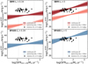 |
Fig. 7 Same as Fig. 6 but for [OIII] 5007 Å. |
| In the text | |
|
Fig. 8 Same as Fig. 6 but for Hα 6563 Å. The dashed green line is the Kennicutt & Evans (2012) relation. |
| In the text | |
|
Fig. A.1 Incident ionising flux, ϕ(H), per energy bin and wavelength bin (CLOUDY models U = −1.00, n = 2, Z = 0.55 Z⊙) for BPASS (blue lines) and SB99 (red lines). The different SFH models are represented with solid (continuous SF) and dashed lines (exponential declining SF τ = 0.3 Gyr). |
| In the text | |
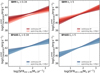 |
Fig. C.1 Same as Fig. 6 but for [NII] 6583Å. |
| In the text | |
|
Fig. C.2 Same as Fig. 6 but for Hβ. |
| In the text | |
Current usage metrics show cumulative count of Article Views (full-text article views including HTML views, PDF and ePub downloads, according to the available data) and Abstracts Views on Vision4Press platform.
Data correspond to usage on the plateform after 2015. The current usage metrics is available 48-96 hours after online publication and is updated daily on week days.
Initial download of the metrics may take a while.