| Issue |
A&A
Volume 693, January 2025
|
|
|---|---|---|
| Article Number | A35 | |
| Number of page(s) | 19 | |
| Section | Extragalactic astronomy | |
| DOI | https://doi.org/10.1051/0004-6361/202451058 | |
| Published online | 03 January 2025 | |
Investigating changing-look active galactic nuclei with long-term optical and X-ray observations
1
Instituto de Estudios Astrofísicos, Facultad de Ingeniería y Ciencias, Universidad Diego Portales, Av. Ejército Libertador 441, Santiago, Chile
2
Institute of Astronomy, National Tsing Hua University, Hsinchu 300044, Taiwan
3
Kavli Institute for Astronomy and Astrophysics, Peking University, Beijing 100871, China
4
Centre for Extragalactic Astronomy, Department of Physics, Durham University, South Road, Durham DH1 3LE, UK
5
School of Physics and Astronomy, Tel Aviv University, Tel Aviv 69978, Israel
6
Department of Astronomy, University of Belgrade – Faculty of Mathematics, Studentski trg 16, 11000 Belgrade, Serbia
7
Hamburger Sternwarte, Universitat Hamburg, Gojenbergsweg 112, D–21029 Hamburg, Germany
8
Indian Center for Space Physics, 466 Barakhola, Netai Nagar, Kolkata 700099, India
9
Eureka Scientific, 2452 Delmer Street Suite 100, Oakland, CA 94602-3017, USA
10
Space Science Institute, 4750 Walnut Street, Suite 205, Boulder, Colorado 80301, USA
⋆ Corresponding author; arghajit.jana@mail.udp.cl
Received:
11
June
2024
Accepted:
13
November
2024
Context. Broad emission lines in the UV/optical spectra of changing-look active galactic nuclei (CLAGNs) appear and disappear on timescales of months to decades.
Aims. We investigate how changing-look (CL) transitions depend on several active galactic nucleus (AGN) parameters, such as the accretion rate, obscuration properties, and black hole mass.
Methods. We studied a sample of 20 nearby optically identified CLAGNs from the BAT AGN Spectroscopic Survey (BASS) using quasi-simultaneous optical and X-ray observations taken in the last ∼40 years.
Results. We find that for all CLAGNs, the transition is accompanied by a change in the Eddington ratio. The CL transitions are not associated with changes in the obscuration properties of the AGNs. CLAGNs are found to have a median Eddington ratio lower than that of the AGNs in the BASS sample in which CL transitions were not detected. The median transition Eddington ratio (the Eddington ratio at which an AGN changes its state) is found to be ∼0.01 for type 1 ↔ 1.8, 1.9, and 2 transitions, which is consistent with the hard ↔ soft state transition in black hole X-ray binaries. Most CL events are constrained to have occurred within 3–4 years, which is considerably shorter than the expected viscous timescale in AGN accretion disks.
Conclusions. The transitions of the optical CLAGNs studied here are likely associated with state changes in the accretion flow, possibly driven by disk instability.
Key words: accretion / accretion disks / galaxies: active / galaxies: nuclei / quasars: supermassive black holes / X-rays: galaxies
© The Authors 2024
 Open Access article, published by EDP Sciences, under the terms of the Creative Commons Attribution License (https://creativecommons.org/licenses/by/4.0), which permits unrestricted use, distribution, and reproduction in any medium, provided the original work is properly cited.
This article is published in open access under the Subscribe to Open model. Subscribe to A&A to support open access publication.
1. Introduction
Active galactic nuclei (AGNs) are powered by the accretion of matter onto supermassive black holes (SMBHs) located at the center of galaxies (e.g., Rees 1988). In the optical/UV, AGNs are generally classified as either type 1 or type 2. Type 1 AGNs show both broad emission lines (BELs; full widths at half maximum > 1000 km s−1) originating in the broad line region (BLR) and narrow emission lines (NELs; full widths at half maximum < 1000 km s−1) originating in the narrow line region (NLR). Type 2 AGNs show only NELs in their UV/optical spectra. Depending on the strength of the BELs, finer classifications (type 1.5, 1.8, and 1.9) can be used (e.g., Osterbrock 1981; Winkler 1992). In X-rays, on the other hand, AGNs are classified based on their obscuration properties, and in particular by their line-of-sight hydrogen column density (NH). AGNs are usually defined as obscured if NH > 1022 cm−2 and unobscured if NH < 1022 cm−2. Furthermore, obscured AGNs can be divided into Compton-thick (CT; NH > 1024 cm−2) and Compton thin (NH < 1024 cm−2) categories.
Generally, type 1 AGNs are found to be unobscured and type 2 AGNs obscured (e.g., Awaki et al. 1991; Koss et al. 2017; Ricci et al. 2017a; Oh et al. 2022). The full width at half maximum of the emission lines is in good agreement with the X-ray obscuration, with type 1–1.8 AGNs having NH < 1021.9 cm−2 and type 2 AGNs having NH > 1021.9 cm−2; however, type 1.9 AGNs show a range of NH (Koss et al. 2017, 2022b). These different classes of AGNs can be explained by the simplified AGN unification model (UM), which is based on the orientation with respect to an anisotropic absorber (e.g., Urry & Padovani 1995; Antonucci 1993; Netzer 2015; Ramos Almeida & Ricci 2017). According to this scheme, type 1s are observed face-on, with the BLR and the NLR visible to the observer, while type 2s are observed edge-on, with the sightline to the BLR blocked by the obscuring material, which leaves only the NLR directly visible to the observer. The intermediate classes of AGNs (type 1.5, 1.8, and 1.9) are thought to be seen through the edge of the obscuring material, where the gas is not optically thick enough to block the entire BLR (e.g., Antonucci 1993; Goodrich 1995; Runco et al. 2016). While the UM provides a good first-order explanation for the different AGN populations, over the past few decades it has been shown that several additional parameters, such as the covering factor of obscuring materials and the accretion rate, can affect the probability of an AGN being observed as obscured or unobscured (e.g., Elitzur & Ho 2009; Ricci et al. 2017b, 2023).
Changing-look AGNs (CLAGNs) show drastic optical and X-ray spectral variability on timescales that range from hours to years and can be generally divided into two classes (see Ricci & Trakhtenbrot 2023, for a recent review). In the UV/optical, CLAGNs transition from type 1 to type 2, or vice versa, on timescales of months to decades. Most of these objects can be considered “changing-state” AGNs (CSAGNs). In X-rays, a different kind of changing-look (CL) event is typically observed. In these objects, the NH show rapid variability on a timescale of hours to years. We refer to these objects as “changing-obscuration” AGNs (COAGNs).
Over the years, many AGNs, such as NGC 1566 (Oknyansky et al. 2019), NGC 3516 (Ilić et al. 2020), Mrk 1018 (Cohen et al. 1986), and Mrk 590 (Shappee et al. 2014), have been found to show CL transitions on a timescale of months to decades. Many of those sources had undergone such transitions more than once. For example, Mrk 1018 entered the type 1.9 state in 1984 (Cohen et al. 1986) and re-brightened again to transition to a type 1 state in 2008 (Shappee et al. 2014). NGC 1566 underwent CL transitions several times in the past 60 years, going between type 1 and type 1.8–1.9 (Shobbrook 1966; Pastoriza & Gerola 1970; Alloin et al. 1986; Baribaud et al. 1992; Oknyansky et al. 2020). NGC 4151 was initially identified as type 1 AGN in the 1970s, but it transitioned to a type 1.8–1.9 state in the 1980s with the disappearance of the broad lines (Osterbrock 1981; Shapovalova et al. 2010). Later, the source transitioned back to a type 1 state as it regained the broad lines. In addition to the local Seyfert galaxies, several higher-redshift quasars have been found to undergo CL transitions (e.g., LaMassa et al. 2015; Merloni et al. 2015; MacLeod et al. 2016). Recently, Zeltyn et al. (2024) identified 116 CLAGNs with repeated spectroscopic observations in the first-year data of the Sloan Digital Sky Survey V (SDSS-V), of which 107 are newly identified CLAGNs. This is the largest sample of CLAGNs reported to date.
The origin of the changing-state (CS) and changing-obscuration (CO) events is still unclear, and many models have been proposed to explain them. Generally, COAGNs are linked to obscuration associated with the clumpiness of the BLR or the circumnuclear molecular dusty gas and dust (e.g., Nenkova et al. 2008a,b; Yaqoob et al. 2015; Ricci et al. 2016; Jana et al. 2020, 2022). CSAGNs are believed to be caused by the change in the accretion rate, which is attributed to local disk instabilities (Stern et al. 2018; Noda & Done 2018) or major disk perturbation, such as tidal disruption events (TDEs; e.g., Merloni et al. 2015; Ricci et al. 2020).
Some CS events have been explained by moving gas clouds and dust that attenuate the BLR emission (e.g., Goodrich 1989, 1995; Zeltyn et al. 2022). However, various problems arise when explaining CS events with obscuration. One needs a large dusty cloud to cover the BLR efficiently, which would take tens of years, assuming reasonable cloud velocity (e.g., LaMassa et al. 2015). However, many CS transitions are observed on a much shorter timescale of months to years (e.g., Denney et al. 2014; Trakhtenbrot et al. 2019; Oknyansky et al. 2019). Additionally, the signature of the obscuration is not observed in the X-ray spectra during or after the transitions (e.g., Denney et al. 2014). In fact, many CSAGNs show the same level of obscuration before and after the transition. Furthermore, many CSAGNs are found to be unobscured, ruling out obscuration as a reason for CS events (e.g., Lyu et al. 2021; Jana et al. 2021). The optical continuum flux also changes with the BEL flux, indicating the accretion flow is a reason for the CS transitions (e.g., Ricci & Trakhtenbrot 2023). A few AGNs, such as NGC 1365 and NGC 7582, showed both CS and CO transitions in the past (e.g., Risaliti et al. 2007; Temple et al. 2023b; Neustadt et al. 2023). However, those transitions are not correlated and are observed on different timescales, indicating independent transitions. Polarimetric studies also suggest that CS transitions are likely not due to changes in the obscuration properties of the source (e.g., Marin 2017; Hutsemékers et al. 2019, 2020).
The BEL flux responds to changes in the ionizing luminosity, which is evident from reverberation studies (e.g., Blandford & McKee 1982; Peterson 1993; Runco et al. 2016; Fonseca Alvarez et al. 2020; Feng et al. 2021a; Oknyansky et al. 2023a). The appearance and disappearance of BELs are examples of the extreme variability of the BLR. In the disk-wind model, the BLR could originate from outflows produced by the accretion disk, which directly connects BELs with the accretion rate (e.g., Emmering et al. 1992; Nicastro 2000; Elitzur & Ho 2009; Temple et al. 2023a). In this framework, the BLR would not be sustained below a certain luminosity, Lcrit < 2.3 × 1040 M82/3 erg s−1 (M8 is the black hole mass in 108 M⊙; Elitzur & Ho 2009). This model suggests that the AGN would follow the transition sequence as type 2 → 1.8, 1.9 → 1.2, 1.5 → 1.0, with an increasing accretion rate (Elitzur 2012; Elitzur et al. 2014).
Local disk instabilities in the accretion disk could also explain CS events (Noda & Done 2018; Sniegowska et al. 2020). The instabilities can be triggered by various mechanisms on different timescales (e.g., Ricci & Trakhtenbrot 2023). In Mrk 1018, the CS transition is explained with the disk instability model (Noda & Done 2018). The CS transition is linked with the soft excess, which is believed to ionize the gas clouds in the BLR. In Mrk 1018, the BEL disappeared when the Eddington ratio (λEdd) decreased from ∼0.08 to ∼0.006, with the primary continuum and soft excess flux reduced by a factor of ∼60 and ∼7, respectively. This transition is tied with the soft-to-hard spectral state transition, similar to black hole X-ray binaries (BHXBs), which occurs at λEdd ≃ 0.01 − 0.02 (e.g., Maccarone 2003; Done et al. 2007; Yang et al. 2015). Similar behavior is also found in other CSAGNs (e.g., Ai et al. 2020; Ruan et al. 2019).
The timescale of CSAGNs is a concerning factor when comparing it with state transitions in BHXBs. Simple mass-scaling relations indicate the viscous timescale for AGNs with masses of ∼106 − 8 M⊙ would be ∼104 − 6 years. However, the timescale would shorten if the accretion disk of AGNs were radiation-pressure-driven, as opposed to the gas pressure-driven accretion disk in BHXBs (Noda & Done 2018). The inclusion of magnetic fields would further shorten the timescale (Feng et al. 2021b). Additionally, various instability mechanisms are suggested to explain the timescale of CS transitions (e.g., Sheng et al. 2017; Sniegowska et al. 2020; Scepi et al. 2021).
Some CSAGNs are associated with external perturbation, such as TDEs. In the CS quasar SDSS J0159+0033, a TDE is believed to have caused the CS transition (Merloni et al. 2015). In the local Universe, the CS transition in 1ES 1927+654 is also found to be caused by a TDE (Trakhtenbrot et al. 2019; Ricci et al. 2020). The CL event in the narrow line Seyfert galaxy SDSS J015804.75–005221.8 is may also be associated with a TDE (Petrushevska et al. 2023).
Temple et al. (2023b) find that a majority of CLAGNs with Swift-BAT light curves showed clear changes in their 14–195 keV X-ray flux at the same time as the change in optical type. This suggests that the majority of CL events in local AGNs are not due to changes in obscuration but must instead be driven by changes in the accretion state. However, detailed spectral modeling across the full X-ray energy range is needed to confirm this, which is one aim of this work.
In this paper we investigate how the optically identified CL transitions depend on several AGN parameters, such as the accretion rate (in terms of λEdd), obscuration (in terms of NH), and black hole mass. Additionally, we provide constraints on the timescale of the CL transitions based on long-term observations. For this purpose, we studied a sample of 20 optically identified CLAGNs using archival quasi-simultaneous optical and X-ray observations taken in the last ∼40 years. In Sect. 2 we present our sample and measurements. In Sect. 3 we present the results of our analysis. In Sect. 4 we discuss our findings. Finally, in Sect. 5 we summarize our results. Throughout the paper, we use Λ cold dark matter cosmology, with the H0 = 70 km s−1 Mpc−1, ΩM = 0.3, and ΩΛ = 0.7.
2. Data and analysis
2.1. Sample selection
We collected our sample of optical CLAGNs from the BAT AGN Spectroscopic Survey (BASS1). Temple et al. (2023b) reported 21 CLAGNs by inspecting multi-epoch optical spectra from BASS DR1 (Koss et al. 2017) and DR2 (Koss et al. 2022a). Of these 21 sources, eight AGNs were reported to be CLAGNs for the first time. To expand our sample, we conducted an extensive literature search of Swift/BAT AGNs. This search revealed an additional 15 CLAGNs that had shown transitions in the last 50 years. Consequently, the total number of optical CLAGNs in our sample increased to 36. All the sources have multi-epoch X-ray observations from the HEASARC data archive2.
Next, we checked if those sources have quasi-simultaneous optical observations with the X-ray observations available in different optical states. We considered quasi-simultaneous observations if the optical and X-ray observations were taken within one year of each other. In this way, our sample is reduced to 20 sources: 16 sources from Temple et al. (2023b) and four CLAGNs from the literature search. The details of the sample are tabulated in Table A.1.
2.2. Optical data and classification
We collected the optical data from the literature. The details of the selected optical observation are presented in Appendix C. We primarily collected information on the optical spectral state from the literature. The optical classifications were based on the scheme of Osterbrock (1981) and Winkler (1992), which is based on the variable flux of Hβ BEL. The classifications are based on the ratio of the fluxes of Hβ BEL and [OIII] NEL (i.e., R =f(Hβ)/f(OIII))as follows:
-
Type - 1: R > 2
-
Type - 1.5: R ∼ 0.33 − 2
-
Type - 1.8: R < 0.33
-
Type - 1.9: No BEL Hβ, Hα BEL.
-
Type - 2: No BELs.
When BEL Hβ and NEL [OIII] flux were available, we calculated the ratio to identify the optical state. When it was not available, we used the classification from the literature.
We note that the optical classifications are not always straightforward, especially when the BELs are weak (type 1.8 or 1.9). Identifying spectral states in historical data, particularly those classified as type 1.8 or 1.9, can indeed be challenging due to issues like poor signal-to-noise ratio (S/N) and spectral resolution. In a low flux state (type 1.8 or 1.9), the BEL flux are often overestimated, which led to misclassification of the state (e.g., Trippe et al. 2010). The type 1–1.5s states show strong BELs and continuum emission and are easily distinguishable from the type 1.8–2.0 states. In this work, we considered type 1–1.5 states as type 1 states.
2.3. Black hole masses
The mass of SMBHs in AGNs has been estimated using BELs and virial prescription. Often, different methods give a different mass value for a particular AGN. Moreover, the CLAGNs are variable; hence, the question arises if the BLR of these CLAGNs are virialized or if CLAGNs follow the same scaling relation as other AGNs. Hence, it is necessary to use the mass value from the literature carefully. Jin et al. (2022) showed that virial estimation of MBH in the brightest epoch (type 1) is consistent with the MBH − σ* estimation in the faint epochs (type-2) for 26 CLAGNs, suggesting the CLAGNs and AGNs follow the same virial scaling relation. Caglar et al. (2023) showed that single epoch virial mass estimation is consistent with the MBH − σ* estimation for type-1 AGNs in BASS, and single epoch measurement are systematically lower by ≃0.12 dex.
In this work, we use the black hole mass from the BASS DR1 or DR2 catalog for 19 sources in our sample (Koss et al. 2017, 2022a). The mass estimation is taken from (i) literature measurements with mega-masers, reverberation mapping, or stellar and gas dynamics; (ii) Hβ or Hα BELs if NH < 1022 cm−2 (from Mejía-Restrepo et al. 2022; iii) Stellar velocity dispersion measurements for all Sy1.9 and Sy2 AGNs (from Koss et al. 2022b), using MBH − σ* relation (from Kormendy & Ho 2013). The mass of NGC 2617 was not available in BASS DR1 or DR2; therefore, we collected the MBH for NGC 2617 from the latest reverberation mapping measurement (Feng et al. 2021a).
2.4. X-ray data analysis
In this work we mainly relied on the X-ray analyses from the literature. However, there are many instances when quasi-simultaneous X-ray observations are available but have yet to be published. We reduced and analyzed those X-ray data, obtained by Swift/XRT, and XMM-Newton. In total, we analyzed 99 observations for 17 sources in the current study. The data reduction technique is described in Appendix B.1.
The X-ray spectra contain several components: primary continuum, soft excess below 2 keV, and reprocessed emission, which consists of a Fe Kα line at ∼6.4 keV and a reflection hump at ∼10 − 40 keV (e.g., Ricci et al. 2017a, 2018a). For the Swift/XRT and XMM-Newton spectra in the 0.5 − 10 keV energy range, we used an absorbed power law model. We used two absorption components; one is for the Galactic absorption, which is fixed at the Galactic absorption value at the source direction. The Galactic absorption is estimated using NH tools from FTOOLS (HI4PI Collaboration 2016)3. The second component is used for the intrinsic source absorption. We used PHABS model for both absorptions components, with ANGR abundances (Anders & Grevesse 1989), and VERNER cross section (Verner et al. 1996). We added a Gaussian line for the Fe Kα line at 6.4 keV and a blackbody component for the soft excess if required.
The spectral analysis is carried out in HEASARC’s spectral analysis software XSPEC4. We obtained a good fit in all spectra, with χ2/degrees of freedom ∼1. From the X-ray data analysis, we obtained the unabsorbed luminosity (LX) and line of sight hydrogen column density (NH). Using the CLUM task, we calculated unabsorbed luminosity in the 2 − 10 keV energy range. The result of the important spectral parameters is tabulated in Appendix C.
2.5. X-ray luminosity
We considered absorption-corrected X-ray luminosity in the 2 − 10 keV energy range. The 2 − 10 keV luminosity (LX) is obtained from the literature or the spectral analysis. We only considered the luminosity of the primary continuum emission, which is thought to originate in the X-ray corona (e.g., Titarchuk 1994; Chakrabarti & Titarchuk 1995; Done et al. 2007).
We considered a Hubble constant H0 = 70 km s−1 Mpc−1 in the present paper; however, in the literature, various values of H0 are considered. We converted those luminosities to the appropriate luminosity consistent with the cosmological parameters used in the present work. When the unabsorbed X-ray flux (FX) was available in the 2 − 10 keV energy range, we calculated the luminosity using,  . Here, dL and Γ are the luminosity distance of the source and photon index of the spectra, respectively. When the 2 − 10 keV unabsorbed flux was not available, we estimated the 2 − 10 keV unabsorbed flux using WEBPIIMS5 tool, with the corresponding NH and the Γ, assuming an absorbed power law continuum. When Γ was not reported, we assumed Γ = 1.8 for the simulation. In this way, we estimated 2 − 10 keV unabsorbed flux for 23 observations for 13 sources when Γ was not available.
2.6. Bolometric correction and Eddington ratio
Once we calculated the LX, we converted it to the bolometric luminosity (Lbol) using bolometric correction factors (kbol). We used Eddington ratio-dependent bolometric correction from Gupta et al. (in prep.). The 2 − 10 keV bolometric correction factor is given by
log kbol = C × (log λEdd)2 + B × log λEdd + A.
Here, C = 0.054 ± 0.034, B = 0.309 ± 0.095 and A = 1.538 ± 0.063. We obtained the Eddington ratios as λEdd = kbol × LX/LEdd = Lbol/LEdd, where LEdd = 1.3 × 1038(MBH/M⊙) erg s−1.
3. Results
3.1. The relation between spectral state and Eddington ratio
The CLAGNs in our sample have been observed across multiple epochs in both the X-ray and optical wavebands, providing us with information on how these sources evolve over time. However, to ensure consistency in our analysis, we focus only on the epochs where quasi-simultaneous observations (< 1 years) in both wavebands were obtained. This approach helps minimize the effects of variability, ensuring that the comparison between X-ray and optical properties reflects the true spectral state of the source.
Figure 1 displays the variation of the Eddington ratio (λEdd) with the spectral state for each CLAGN in our sample. Our analysis reveals a significant correlation between the optical spectral state and the Eddington ratio for all 20 sources. Specifically, we observe that the CL transitions between type 1 and type 2 states are tightly linked to changes in their accretion rates. When the Eddington ratio increases, the AGNs tend to transition toward a type 1 state, characterized by stronger BELs and brighter continuum emission. Conversely, when the Eddington ratio decreases, the sources tend to transition toward a type 2 state, where BELs are weaker or absent, and the continuum is dimmer. This pattern indicates that the accretion rate plays a crucial role in driving the CL phenomenon, with higher accretion rates leading to the type 1 state and lower accretion rates leading to the type 2 state.
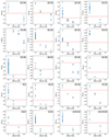 |
Fig. 1. Distribution of λEdd with the spectral states for each source. The horizontal dashed red lines in each panel represent the transition Eddington ratio ( |

To quantify this relationship further, we calculate both the mean and median values of the Eddington ratio (λEdd) for each spectral state. This is shown in Fig. 2, where the blue circles represent the median values of λEdd at each state. A clear trend is observed in the figure: both the mean and median Eddington ratios increase as the CLAGNs transition toward the type 1 state and decrease as they transition toward the type 2 state. The mean and median Eddington ratios for each spectral state are provided in Table 1.
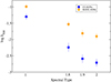 |
Fig. 2. Median Eddington ratio in each spectral state. The blue circles represent the median λEdd for CLAGNs. The orange diamonds represent the median λEdd for the other AGNs from the BASS sample for which CL transitions were not detected. |
Mean and median Eddington ratio (λEdd) and hydrogen column density (NH) for CLAGNs and other AGNs from BASS for which CL transitions have not been detected.
3.2. Relation between spectral state and X-ray obscuration
The obscuration of AGNs is commonly characterized by the line-of-sight hydrogen column density (NH) along the line of sight. In Fig. 3 we examine the variation of NH as a function of the optical spectral state for each source in our sample. Interestingly, we did not see any a clear correlation between the spectral state and NH for most of the sources. Our results suggest that obscuration is not the dominant factor for the majority of the AGNs in our sample.
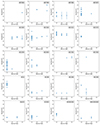 |
Fig. 3. Variation in NH as a function the spectral state for our sample. In NGC 526A, NGC 7603, and HE 1136–2304, the NH value is only available for type 2, type 1.8, and type 1.0 states, respectively. |
A notable exception to this trend is NGC 1365, for which we observe an intriguing behavior. This source appeared to transition into a type 2 state while simultaneously being in a CT X-ray state, characterized by an extremely high column density of obscuring material (NH > 1024 cm−2). However, NGC 1365 shows rapid NH variability on a timescale of days, which is not related to the optical state transitions. The detailed study found that the CL transition in this source is led by the change of accretion rate, not obscuration (see Sect. 4.2 for details).
To further analyze the role of obscuration in AGN transitions, we calculated the median values of NH for each spectral state. Figure 4 displays the median NH for type 1, type 1.8, type 1.9, and type 2.0 states. The blue circles represent the median NH for the CLAGNs at each spectral state. The median NH is found to be non-variable with respect to the spectral state. The mean and median values of NH for each spectral state are presented in Table 1. The median NH was found to be log(NH/cm2) = 21.35 ± 0.15 in type 1 states. For type 1.8, type 1.9, and type 2 states, the medians are log(NH/cm2) = 21.88 ± 0.14, 21.61 ± 0.08, and 22.32 ± 0.11, respectively.
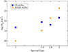 |
Fig. 4. Median NH in each spectral state. The blue circles and orange diamonds represent the CLAGNs in our sample and other AGNs from the BASS sample, respectively. |
3.3. Distribution of spectral states
To further investigate the dependence of spectral state on both the λEdd and NH, we analyzed the distribution function of each spectral state as a function of these parameters. In Figure 5, we present the fraction of CLAGNs in different spectral states as a function of λEdd. To calculate these distributions, we divided the range of log λEdd from −0.5 to −3.5 into bins with a width of Δlog λEdd = 0.5. The fraction of CLAGNs in each spectral state within each bin was then calculated, providing insight into the behavior of AGNs across this range of accretion rates. The uncertainty in the fraction of CLAGNs for each spectral state was estimated using the 16th and 84th quantiles of a binomial distribution, following the method outlined by Cameron (2011).
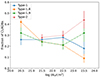 |
Fig. 5. Fraction of CLAGNs in different spectral states for different NH. The blue circles, orange squares, green diamonds, and red triangles represent the type 1, 1.8, 1.9, and 2.0 states, respectively. |
The f1 displays a clear increase with λEdd, while f2 shows the opposite behavior. Neither f1.9 nor f1.8 showed any clear variation. The observed trend of a fraction of CLAGNs in each spectral state also shows that CLAGNs transition toward a type 1 state for increasing λEdd.
In Fig. 6 we examine the distribution of spectral states as a function of NH. Here, the range of log NH from 20.0 to 24.0 is divided into bins with a width of Δlog(NH/cm2) = 0.5. Similar to the Eddington ratio distribution, we calculated the fraction of CLAGNs in each spectral state within each bin.
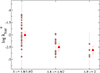 |
Fig. 6. Fraction of CLAGNs in different spectral states for different λEdd. The blue circles, orange squares, green diamonds, and red triangles represent the fraction of CLAGNs in type 1, type 1.8, type 1.9, and type 2 states, respectively. |
With increasing log NH, we observe a decrease in the fraction of f1 and f1.8, suggesting that these states are more commonly associated with lower levels of obscuration. Interestingly, the fraction of f1.9 does not show any clear variation with NH. On the other hand, the fraction f2 increases with increasing NH, consistent with the idea that type 2 states are typically more heavily obscured than type 1 states. However, considering the uncertainties, the f1 and f2 remain constant with NH.
3.4. The transition Eddington ratio
In our sample of 20 optically identified CLAGNs, we observe that transitions between spectral states are driven primarily by changes in the accretion rate. To investigate the physical mechanism behind these transitions, we estimated the transition Eddington ratio ( ) for each spectral change in each source. The AGNs undergo transitions between spectral states at
  .
.
The  for each state transition is computed as follows: we first identify the range of Eddington ratios associated with the transition by determining the highest λEdd value of the lower state (type 2s) and the lowest λEdd value of the higher state (type 1s). The midpoint of this range is then considered as the transition Eddington ratio,
  , for that specific transition. The uncertainty in
  is derived by calculating the difference between the highest or lowest values of the range and the mid-point.
To further quantify the transition points between spectral states, we estimate the median  , corresponding to different spectral state transitions. We estimated the median by applying the bootstrap method. For each bootstrap sample, the median was calculated. This process was repeated 1000 times to generate the distribution of medians. From this distribution, we calculated the median
  for each transition. In Fig. 7 we present
  for the various spectral state transitions observed in our CLAGN sample. The gray circles represent the individual
  values for each CL transition, while the red triangles indicate the median values of
  for each type of transition.
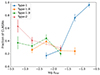 |
Fig. 7. Transition Eddington ratio ( |


For transitions type 1 ↔ 1.8/1.9/2, we find that the median value of  is −2.01 ± 0.16. This suggests that AGNs typically transition from a type 1 state to a type 1.8, 1.9, or 2 state when their accretion rate drops below
  .
.
For the transitions, such as from type 1.8 ↔ 1.9/2 and from type 1.9 ↔ 2.0, the median values of  are −2.50 ± 0.18 and −2.62 ± 0.19, respectively. Interestingly, the transition Eddington ratios for these states do not differ significantly, and the values are consistent within the uncertainties. It has been previously shown that the classifications of type 1.8, type 1.9, and type 2.0 AGNs can be somewhat ambiguous, due to the faintness of the BEL flux in these states (e.g., Trippe et al. 2008, 2010). The spectral lines in these states can be weak and difficult to distinguish, leading to potential misclassifications. As a result, type 1.8, type 1.9, and type 2 states may not always be correctly categorized, which could explain the similar
  values observed for transitions between these states. The median values of
  for each spectral state transition are provided in Table 2.
Median transition Eddington ratio ( ).
).
4. Discussion
4.1. CLAGNs: Accretion versus obscuration
In our sample of 20 optically identified CLAGNs, we observed a clear correlation between the spectral state of each CLAGN and the Eddington ratio (see Fig. 1). We observed that CLAGNs tend to transition to a type 1 spectral state as the Eddington ratio increases, and conversely, they transition to a type 2 state as the Eddington ratio decreases. When we calculate the median λEdd at each spectral state, type 1s states are found to have a higher λEdd than type 2 states (Fig. 6). The distribution function f1 (fraction of CLAGNs in type 1 state) also shows a clear increase as a function of λEdd, indicating that AGNs are more likely to be in a type 1 state when their accretion rate is higher. Conversely, the fraction f2 demonstrates the opposite behavior, with the fraction of type 2 AGNs decreasing as the Eddington ratio increases. This indicates that AGNs are more likely to be in a type 2 state when their accretion rate is lower. This implies that the observed transitions in spectral characteristics are strongly tied to variations in the accretion rate, with AGNs transitioning between spectral states with the change in the accretion rate.
We also checked the relation between optical spectral state and X-ray obscuration for CLAGNs in our sample. No significant relation was detected between the spectral state and the line-of-sight column density (see Fig. 3). While the UM of AGNs posits that type 1 AGNs are typically unobscured (low NH) and type 2 AGNs are obscured (high NH), our results show that this relation does not hold for the majority of the CLAGNs in our sample. When we calculate the median NH at each spectral state, we did not find a significant variation of NH with the spectral state (see Fig. 4). The distribution of spectral state as a function of NH (relation between f1, f2 and NH) might suggest that the optical state could be related to NH (see Fig. 5). This would be consistent with the UM where type 1s are typically unobscured and type 2s are typically obscured. However, when we check how the spectral state changes with NH for individual sources (see Fig. 3), we clearly see that there is no relation between these two quantities for 19 of the 20 sources of our sample. Moreover, the changes in f1 and f2 with NH are within uncertainties, indicating that the optical state is not directly tied to the X-ray obscuration. Hence, consistent with the results of Temple et al. (2023b), there is no clear indication of NH being the driver of the CL transitions.
Instead, the CLAGNs in our sample appear to change their optical and X-ray properties due to intrinsic changes in the accretion flow rather than external factors such as varying obscuration or material along the line of sight. This behavior supports the idea that optically identified CLAGNs can be classified as CSAGNs, where the optical state transitions are directly linked with the variation of accretion flow around SMBHs.
4.2. CLAGNs with CS and CO transition
Two CLAGNs in our sample, NGC 1365 and NGC 7582, have undergone both CS and CO transitions (Risaliti et al. 2005; Piconcelli et al. 2007; Bianchi et al. 2009; Temple et al. 2023b). These two sources provide a unique opportunity to investigate the potential relationship between the CS and CO transitions. In our analysis, we explored whether the CS and CO transitions are connected.
NGC 1365. NGC 1365 was observed in the CT state in July 2010, and optical observations carried out in September 2010 revealed that the source was in a type 2 state, while accreting at log λEdd ∼ −1.56 (Brenneman et al. 2013). In December 2012, the source transitioned to a type 1.8 state (Lena et al. 2016). The X-ray observation found the source in a Compton thin state at this time, with increasing log λEdd ∼ −1.36 (Walton et al. 2013). From this, it may seem that both λEdd and NH are responsible for the CL transition in NGC 1365. However, NGC 1365 showed rapid absorption variability on a timescale of days (Risaliti et al. 2007). The obscuring clouds are small and found to be located in the BLR, which suggests that the obscuring material cannot block the BLR. Mondal et al. (2022) suggest that the obscuration might be attributed to a failed wind, driven by the variable accretion rate. However, the wind can only contribute to the obscuration of the X-ray source and not affect our view of the BLR.
NGC 7582. NGC 7582 showed a variable NH over the years, with a CT state observed several times (Lefkir et al. 2023, and references therein). The NH varied in the ∼8 − 130 × 1022 cm−2 range over the last ∼40 years, undergoing several CO transitions. In 2005, XMM-Newton found the source in a CT a state with NH = (1.3 ± 0.1)×1024 cm−2 (Piconcelli et al. 2007). In April 2007, the source was found in Compton thin state with NH = (3.3 ± 0.5)×1023 cm−2. Within six months, the source transitioned again to a CT state [NH = (1.2 ± 0.2)×1024 cm−2]. In 2012, NGC 7582 was found in a Compton-thin state and transitioned back to a CT state in 2014 (Braito et al. 2017). In 2016, the source was again found in Compton-thin state (Lefkir et al. 2023).
Unfortunately, we do not have simultaneous optical observations during all the CO transitions. However, the NH variations were observed when the source was in the type 1.9/2 state, and only λEdd was observed to correlate with the optical spectral state in this object, confirming the idea that CO & CS transitions are independent and that the varying accretion rate drives the optical state transition.
4.3. Timescale of the CL transitions
The observed timescales of the CL transitions (tCL) challenge our understanding of the accretion properties of SMBHs. Generally, CL transitions are seen on timescales of months to decades (e.g., Denney et al. 2014; Shapovalova & Popović 2019; Gezari et al. 2017; Trakhtenbrot et al. 2019; Ricci & Trakhtenbrot 2023; Zeltyn et al. 2022). In our current study, we focus on a sample of optically identified CLAGNs, utilizing optical data accumulated over the past 40 years. By comparing the time intervals between the first and last epochs of observations in different spectral states, we were able to place upper limits on the CL transition timescales for each source. These upper limits provide interesting constraints on the temporal evolution of the accretion processes in AGNs. Figure 8 displays the distribution of our upper limits on the CL transition timescales for our sample. We only considered the timescale for the type 1 ↔ 1.8, 1.9, or 2 transition. The timescales cover a range from a few weeks to ∼20 years. We find that the median of the upper limit of the transition timescale is 3 − 4 years, which is consistent with previous findings for CLAGNs in BASS (Temple et al. 2023b).
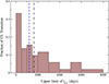 |
Fig. 8. Distribution of the upper limit of the timescale for the CL events. The vertical dashed blue and dot-dashed black lines represent the median and mean values of the distribution, respectively. |
The standard thin disk model predicts the radial inflow timescale or viscous timescale to be tvis≃ 400  (α/0.03)−1(R/150rg)3/2M8 years (Shakura & Sunyaev 1973; Noda & Done 2018; Stern et al. 2018; Ricci & Trakhtenbrot 2023). Here, H is the disk height at distance R, α is the viscosity parameter, and M8 is the mass of the SMBH in 108 M⊙. For AGNs of mass ∼106 − 8 M⊙, tvis would be ∼104 − 6 years, which is considerably longer than the observed transition time. The dynamical timescale (tdyn) is typically shorter than the observed timescale. The dynamic timescale of the gas is related to the orbital motion of the gas around the black hole and is given by tdyn ≃ 10(R/150 rg)3/2M8 days. The thermal timescale (tth) or the timescale associated with the heating or cooling of the disk is tth ≃ tdyn/α ≃ (α/0.03)−1(R/150 rg)3/2M8 years. Such a timescale is generally associated with the stochastic variability of the AGN (Kelly et al. 2009). Another relevant timescale is the timescale associated with the radial propagation of the heating and cooling front (tfront; Osaki 1996; Dubus et al. 2001). The cooling front timescale is
  years (Stern et al. 2018).
In Fig. 9 we show several key theoretical timescales relevant to accretion disk physics, namely, viscous time (tvis), thermal time (tth), dynamic time (tdyn), and heat/cold front timescale (tfront), along with the upper limit of the observed CL transition time (tCL) as a function of MBH. For our calculations we considered a disk-aspect ratio H/R = 0.2, a viscosity parameter α = 0.1, and R ∼ 150 rg (i.e., the typical emission zone for UV-optical continuum (e.g., Noda & Done 2018; Stern et al. 2018).
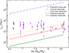 |
Fig. 9. Relation of the transition timescale (tCL) with the black hole mass in logarithmic scale (log MBH). The downward pointing purple arrows represent the upper limit of the transition time for all CL transitions in our study. The dashed-dot-dot-dashed blue, dot-dashed orange, dashed red, and solid green lines represent the viscous time, cold front propagation time, thermal time, and dynamic time, respectively. The timescales are calculated assuming a disk aspect ratio H/R = 0.2 and a viscosity parameter α = 0.1. |
Figure 9 clearly shows that all transitions occurred on a shorter timescale than tvis. Most transition timescales are consistent with the thermal, cooling front, and dynamic timescales. These timescales suggest that thermal instabilities or the propagation of heating and cooling fronts in the accretion disk may play a significant role in driving CL transitions. Also, some transition timescales could be consistent with the dynamic time. Here, we also note that one may reduce the tvis if the accretion disk is inflated. This could occur if the total opacity of the disk increases due to heavy elements, which raise both the temperature and scale height (Jiang et al. 2016). Magnetic torques in the inner disk can also heat and expand the disk structure (Agol & Krolik 2000), while magnetic pressure in the upper layers of the disk contributes to further disk inflation (Dexter & Begelman 2019). Additionally, magnetically driven disk winds can remove the angular momentum, further shortening the tvis (Feng et al. 2021b).
Interestingly, in IRAS 23226–3843, a transition occurred on a timescale of ∼14 days (Kollatschny et al. 2023), which could be associated with the dynamical time. This indicates that, in some cases, CL transitions could be driven by dynamic processes within the inner accretion disk. Such fast transitions are rare but highlight the need to consider multiple physical mechanisms that could influence the CL phenomena. We note that some transitions could be associated with the thermal timescales and others with the dynamic timescales. Establishing precise transition timescales is crucial for identifying the underlying physical processes.
4.4. Comparing CLAGNs with other AGNs in BASS
In our sample of CLAGNs, the median value of the log λEdd for type 1, 1.8, 1.9, and 2.0 are −1.30 ± 0.09, −2.24 ± 0.14, −2.59 ± 0.13 and −2.71 ± 0.12, respectively. For un-beamed (non-blazar) AGNs in the BASS sample in which CL transitions were not detected (hereafter BASS AGNs), Koss et al. (2022a) found the median value of log λEdd for type 1, 1.8, 1.9, and 2.0 are −0.99 ± 0.07, −1.53 ± 0.08, −1.81 ± 0.11 and −1.90 ± 0.09, respectively. In every spectral state, CLAGNs have a lower λEdd than AGNs in the BASS (see Fig. 2).
We also compared the median λEdd for CLAGNs with that of other AGNs from the BASS survey using a redshift-matched sample. To do this, we divided the CLAGNs into three redshift bins: z = 0 − 0.01, 0.01 − 0.03, and 0.03 − 0.06, containing eight, seven, and five CLAGNs, respectively. For each bin, we calculated the median λEdd of the CLAGNs. Similarly, we constructed three corresponding redshift bins for other BASS AGNs, randomly selecting the same number of AGNs in each bin (i.e., we randomly selected eight, seven, and five AGNs from BASS at redshift bins of z = 0 − 0.01, 0.01 − 0.03, and 0.03 − 0.06, respectively). The median λEdd for these AGNs was then estimated using a bootstrapping method with 1000 realizations. This allowed us to determine the median λEdd for both the CLAGNs and the other BASS AGNs for each spectral state. The variation in the median λEdd with redshift for both CLAGNs and other AGNs is shown in Fig. 10. The panels display the median Eddington ratio for type 1, type 1.8, type 1.9, and type 2 AGNs in the top left, top right, bottom left, and bottom right panels, respectively. In all spectral states and redshift bins, we consistently found that CLAGNs exhibit a lower Eddington ratio compared to other BASS AGNs that did not show CL transitions. We employed the Anderson-Darling (AD) test to compare the distributions of the Eddington ratio for CLAGNs and other BASS AGNs across different spectral states. Our results indicate that the distributions are significantly different in each state, with a p-value of pAD < 0.001. This finding remained consistent when we repeated the analysis using the redshift-matched distributions for CLAGNs and BASS AGNs. Our findings that CLAGNs tend to have a lower λEdd than other AGNs in the BASS, agree with previous studies (Zeltyn et al. 2024; Wang et al. 2024). In the SDSS-V survey, the median λEdd in CLAGNs is found to be ∼0.025, while other AGNs have a median value of λEdd ∼0.043 (Zeltyn et al. 2024). The CL quasars are observed to have a lower λEdd compared to the general population of the quasar in SDSS (MacLeod et al. 2019). Temple et al. (2023b) also found a similar result from the BAT-selected CLAGN sample in the local Universe.
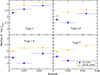 |
Fig. 10. Comparison of the median Eddington ratio (λEdd) of CLAGNs and other AGNs in the BASS sample with redshifts. Three bins are constructed, for redshifts Δz = 0 − 0.01, 0.01 − 0.03, and 0.03 − 0.06; these bins contain eight, seven, and five CLAGNs, respectively. For the other AGNs from BASS, each bin is constructed by randomly selecting the same number of AGNs as CLAGNs in the same bin and bootstrap-processed with 1000 realizations. The median λEdd for type 1, type 1.8, type 1.9, and type 2 with redshifts are show in the top-left, top-right, bottom-left and bottom-right panels, respectively. |
We also obtain a median NH for each spectral state for the CLAGNs in our sample. Figure 4 shows the median NH for CLAGNs and other AGNs in each spectral state. For BASS AGNs, the median NH increases as the AGNs transition toward a type 2 state, which is consistent with the UM of AGNs. Comparing CLAGNs with other AGNs in BASS (Ricci et al. 2017a), we find that the median NH for type 1 and 1.8 for the CLAGNs are higher than other AGNs. For CLAGNs, the median varies in the range log(NH/cm2) = 21.45 − 21.88. For other AGNs in BASS, the range of the median is log(NH/cm2) = 20.00 − 23.27. The range of NH suggests that NH tends to be less variable for CLAGNs than other AGNs in the BASS, indicating that the CL transition does not depend on the obscuration properties. Using the AD test, we found significant differences in the distributions in all the spectral states, with p-values < 0.001.
4.5. The physical mechanisms responsible for CL transitions
From our study of 20 optically identified CLAGNs using quasi-simultaneous optical and X-ray observations, we find that changes in the accretion flow are the primary driver of CL transitions in all sources, while we did not detect any significant variations in the obscuration properties of these CLAGNs associated with the transitions (see Sects. 3.1 and 3.2). This suggests that the optical CLAGNs in our sample can indeed be classified as CSAGNs, where changes in the accretion flow rather than external factors, like obscuration, dictate the transitions between spectral states.
In recent years, several models have been proposed to explain these CS transitions in AGNs (Elitzur 2012; Noda & Done 2018; Sniegowska et al. 2020). One prominent model is the disk-wind model for the BLR (Nicastro 2000; Elitzur & Ho 2009; Elitzur et al. 2014), which predicts that the BLR should disappear when the AGN luminosity falls below a critical value. This model relies on the idea that radiation pressure driven wind is responsible for the formation of the BLR, and if the bolometric luminosity (Lbol) falls below a critical value,  erg/s, the BLR would no longer be sustained. As a result, the BLR vanishes, and the AGN transitions into a type 2 state. This model provides an effective way to explain why some AGNs undergo transitions from type 1 to type 2, linking the appearance of the BLR directly to the strength of the accretion-powered radiation.
However, in our study, we found that this model does not fully explain the observed CL transitions. Specifically, we found that in our sample of 20 optical CLAGNs, all sources have bolometric luminosities well above the critical threshold predicted by the disk-wind model, in their type 2 states. This suggests that the disk-wind model is not sufficient to explain all CL transitions, particularly those where the AGN retains a high bolometric luminosity. The disappearance of the BLR in these cases likely involves more complex processes tied to the dynamics of the accretion flow or changes in the structure of the central regions of the AGN, rather than simply a drop in luminosity. This challenges the universality of the disk-wind model and points to the need for alternative models that can account for the complex interplay between accretion processes and BLR formation in AGNs undergoing CL transitions.
The disk instability model also provides a key framework for understanding the CS transitions in AGNs, linking these transitions to the spectral state changes commonly observed in BHXBs (Noda & Done 2018; Ross et al. 2018; Ai et al. 2020). In BHXBs, state transitions are well-studied, and the change in accretion geometry during these transitions leaves a distinct imprint on the correlation between the photon index (Γ) and the Eddington ratio (λEdd; e.g., Yang et al. 2015; Yan et al. 2020). This Γ − λEdd correlation acts as a diagnostic of the accretion state, providing valuable insight into the physical mechanisms governing the behavior of both BHXBs and AGNs.
In BHXBs, the Γ − λEdd correlation behaves differently depending on whether the source is in a high-soft or low-hard state. During the high-soft state, where the system is dominated by thermal emission from the accretion disk, a positive correlation between Γ and λEdd is typically observed. In this state, increasing accretion rate leads to efficient cooling in the X-ray corona, which produces softer spectra, leading to an increase in Γ (Yang et al. 2015; Yan et al. 2020; Jana 2022). Conversely, in the low-hard state, a negative correlation between Γ and λEdd is observed. In this state, the accretion disk recedes, and the inner accretion flow is replaced by a hot radiatively inefficient flow (Zdziarski et al. 2014; Yuan et al. 2015). The seed photons are supplied by the synchrotron emission in the hot flow or jets. As the accretion rate decreases, the degree of synchrotron self-absorption decreases, which leads to softer spectra (i.e., increases in Γ). The critical Eddington ratio at which this correlation flips is found to be around λEdd ∼ 0.01, marking the transition between the high-soft and low-hard states.
A similar behavior in the Γ − λEdd relation is also observed in AGNs, suggesting that the accretion physics in AGNs and BHXBs may be fundamentally similar. In AGNs, this transition in the Γ − λEdd correlation typically occurs at λEdd ≈ 0.01 − 0.02 (Noda & Done 2018; Ruan et al. 2019; Jana et al. 2023), which is comparable to the value observed in BHXBs. Studies of CL quasars have further supported this connection, showing that quasars evolve from a bright, high-accretion state to a faint, low-accretion state, and vice versa, with the transition also occurring at λEdd ≈ 0.01 (Ruan et al. 2019; Jin et al. 2021). This suggests that the same underlying physical mechanisms, likely driven by instabilities in the accretion disk, are responsible for the observed state changes.
In the present work, we have found that the median Eddington ratio for CLAGNs during state transitions,  . This value is consistent with the soft-to-hard state transition Eddington ratio seen in BHXBs (Maccarone 2003; Jana 2022), further supporting the hypothesis that disk instabilities are the primary drivers of these transitions in CLAGNs. Specifically, these instabilities likely alter the structure and geometry of the accretion flow, leading to changes in the accretion rate and, consequently, the spectral state of the CLAGNs.
Our sample does not include extreme low accreting (λEdd < 10−4) or high accreting AGNs (super Eddington source, λEdd > 1). For instance, 1ES 1927+654 was found to be accreting at super Eddington rate during the CL transitions (Trakhtenbrot et al. 2019; Ricci et al. 2020, 2021; Li et al. 2022a), with the transition driven by the change in the accretion rate (Li et al. 2024b,a). On the other hand, several low luminosity CL LINERs low ionization nuclear emission line region galaxies have been detected (Schimoia et al. 2015). We will study these objects in detail elsewhere.
5. Summary and conclusions
We conducted a comprehensive study of 20 optically identified CLAGNs in the local Universe (z < 0.06) using quasi-simultaneous optical and X-ray observations from BASS. This multiwavelength approach allowed us to explore the connection between changes in the accretion processes and the spectral properties of these AGNs over time. The quasi-simultaneous X-ray and optical data provide crucial insights into the physical mechanisms driving the observed transitions. We utilized optical and X-ray data in the literature from the last 40 years. The optical spectral state was classified using optical observations, while the Eddington ratio and line-of-sight hydrogen column density were estimated from X-ray observations. We investigated the dependence of CL transitions on different AGN parameters, such as the Eddington ratio, obscuration, and black hole mass. The key findings of our work are summarized as follows:
-
The CL transitions are likely caused by changes in the accretion flow. In our sample, all sources show type 1 → 2 transitions as λEdd decreases, and vice versa.
-
The CL transitions are not related to obscuration properties, confirming the idea that CS transitions are solely led by changes in the accretion flow.
-
Our CLAGNs have a lower accretion rate than the AGNs from the BASS sample for which CL transitions have not been detected.
-
The median transition Eddington ratio for type 1 ↔ 1.8, 1.9, or 2 is
 , or λEdd ≈ 0.5 − 2% of Eddington limit. The
  is consistent with the prediction of the disk instability model (e.g., Noda & Done 2018). The
  is consistent with the transition Eddington ratio of the soft↔hard state transition Eddington ratio in BHXBs.
 -
We could only estimate the upper limit of the CL transition times of our sample. We find that the majority of CL transitions in our sample occurred within 3 − 4 years.
Currently, the main challenge in the study of CLAGNs is low cadence observations, which are not ideal for studying the physics underlying the transition mechanism. This will change with the advent of large photometric (LSST; Ivezić et al. 2019) and spectroscopic surveys in the optical ((SDSS-V, Kollmeier et al. 2017; 4MOST, de Jong et al. 2019)) and wide-field surveys in X-rays ((eROSITA; Merloni et al. 2020); and (Einstein probe, Yuan et al. 2015)) and UV wavelengths (with ULTRASAT; Shvartzvald et al. 2023). These surveys are expected to identify a large number of new CLAGNs, as well as new transitions of known CLAGNs, which will help us understand the physical mechanism of the spectral transitions in greater detail. Additionally, in the future, we will also investigate the connection of CLAGNs with state transitions in BHXBs using archival multiwavelength observations.
Data availability
All the data used in the paper are publicly available. Tables C.1–C.20 are available at the CDS via anonymous ftp to cdsarc.cds.unistra.fr (130.79.128.5) or via https://cdsarc.cds.unistra.fr/viz-bin/cat/J/A+A/693/A35.
Acknowledgments
We acknowledge the reviewer for their very detailed and helpful comments on the manuscript. AJ acknowledges support from FONDECYT Postodoctoral fellowship (3230303). AJ and HK acknowledge the support of the grant from the National Science and Technology Council of Taiwan with the grand numbers MOST 110-2811-M-007-500, MOST 111-2811-M-007-002, and NSTC 112-2112-M-007-053. CR acknowledges support from Fondecyt Regular grant 1230345, ANID BASAL project FB210003 and the China-Chile joint research fund. MJT acknowledges support from STFC grant ST/X001075/1 and a FONDECYT Postdoctoral fellowship (3220516). BT is supported by the European Research Council (ERC) under the European Union’s Horizon 2020 research and innovation program (grant agreement number 950533) and from the Israel Science Foundation (grant number 1849/19). YD is supported by a FONDECYT postdoctoral fellowship (3230310). DI acknowledges funding provided by the University of Belgrade – Faculty of Mathematics (the contract 451-03-66/2024-03/200104) through the grant of the Ministry of Science, Technological Development and Innovation of the Republic of Serbia.
References
- Afanasiev, V. L., Popović, L. Č., Shapovalova, A. I., Borisov, N. V., & Ilić, D. 2014, MNRAS, 440, 519 [Google Scholar]
- Agol, E., & Krolik, J. H. 2000, ApJ, 528, 161 [NASA ADS] [CrossRef] [Google Scholar]
- Agüero, E. L., Díaz, R. J., & Bajaja, E. 2004, A&A, 414, 453 [NASA ADS] [CrossRef] [EDP Sciences] [Google Scholar]
- Ai, Y., Dou, L., Yang, C., et al. 2020, ApJ, 890, L29 [NASA ADS] [CrossRef] [Google Scholar]
- Allen, M. G., Dopita, M. A., Tsvetanov, Z. I., & Sutherland, R. S. 1999, ApJ, 511, 686 [NASA ADS] [CrossRef] [Google Scholar]
- Alloin, D., Pelat, D., Phillips, M. M., Fosbury, R. A. E., & Freeman, K. 1986, ApJ, 308, 23 [NASA ADS] [CrossRef] [Google Scholar]
- Anders, E., & Grevesse, N. 1989, Geochim. Cosmochim. Acta, 53, 197 [Google Scholar]
- Antonucci, R. 1993, ARA&A, 31, 473 [Google Scholar]
- Antonucci, R. R. J., & Cohen, R. D. 1983, ApJ, 271, 564 [Google Scholar]
- Aretxaga, I., Joguet, B., Kunth, D., Melnick, J., & Terlevich, R. J. 1999, ApJ, 519, L123 [NASA ADS] [CrossRef] [Google Scholar]
- Awaki, H., Kunieda, H., Tawara, Y., & Koyama, K. 1991, PASJ, 43, L37 [NASA ADS] [Google Scholar]
- Baribaud, T., Alloin, D., Glass, I., & Pelat, D. 1992, A&A, 256, 375 [NASA ADS] [Google Scholar]
- Bennert, N., Jungwiert, B., Komossa, S., Haas, M., & Chini, R. 2006, A&A, 459, 55 [NASA ADS] [CrossRef] [EDP Sciences] [Google Scholar]
- Bentz, M. C., Walsh, J. L., Barth, A. J., et al. 2009, ApJ, 705, 199 [NASA ADS] [CrossRef] [Google Scholar]
- Bianchi, S., Piconcelli, E., Chiaberge, M., et al. 2009, ApJ, 695, 781 [Google Scholar]
- Blandford, R. D., & McKee, C. F. 1982, ApJ, 255, 419 [Google Scholar]
- Braito, V., Reeves, J. N., Bianchi, S., Nardini, E., & Piconcelli, E. 2017, A&A, 600, A135 [EDP Sciences] [Google Scholar]
- Brenneman, L. W., Risaliti, G., Elvis, M., & Nardini, E. 2013, MNRAS, 429, 2662 [CrossRef] [Google Scholar]
- Caglar, T., Koss, M. J., Burtscher, L., et al. 2023, ApJ, 956, 60 [NASA ADS] [CrossRef] [Google Scholar]
- Cameron, E. 2011, PASA, 28, 128 [Google Scholar]
- Chakrabarti, S., & Titarchuk, L. G. 1995, ApJ, 455, 623 [NASA ADS] [CrossRef] [Google Scholar]
- Chen, Y.-J., Bao, D.-W., Zhai, S., et al. 2023, MNRAS, 520, 1807 [NASA ADS] [CrossRef] [Google Scholar]
- Cohen, R. D., Rudy, R. J., Puetter, R. C., Ake, T. B., & Foltz, C. B. 1986, ApJ, 311, 135 [NASA ADS] [CrossRef] [Google Scholar]
- de Jong, R. S., Agertz, O., Berbel, A. A., et al. 2019, The Messenger, 175, 3 [NASA ADS] [Google Scholar]
- Denney, K. D., De Rosa, G., Croxall, K., et al. 2014, ApJ, 796, 134 [Google Scholar]
- de Vaucouleurs, G. 1973, ApJ, 181, 31 [NASA ADS] [CrossRef] [Google Scholar]
- Dexter, J., & Begelman, M. C. 2019, MNRAS, 483, L17 [NASA ADS] [CrossRef] [Google Scholar]
- Done, C., Gierliński, M., & Kubota, A. 2007, A&ARv, 15, 1 [Google Scholar]
- Doroshenko, V. T., & Sergeev, S. G. 2003, A&A, 405, 909 [NASA ADS] [CrossRef] [EDP Sciences] [Google Scholar]
- Dubus, G., Hameury, J. M., & Lasota, J. P. 2001, A&A, 373, 251 [NASA ADS] [CrossRef] [EDP Sciences] [Google Scholar]
- Edmunds, M. G., & Pagel, B. E. J. 1982, MNRAS, 198, 1089 [NASA ADS] [CrossRef] [Google Scholar]
- Elitzur, M. 2012, ApJ, 747, L33 [Google Scholar]
- Elitzur, M., & Ho, L. C. 2009, ApJ, 701, L91 [Google Scholar]
- Elitzur, M., Ho, L. C., & Trump, J. R. 2014, MNRAS, 438, 3340 [Google Scholar]
- Emmering, R. T., Blandford, R. D., & Shlosman, I. 1992, ApJ, 385, 460 [NASA ADS] [CrossRef] [Google Scholar]
- Evans, P. A., Beardmore, A. P., Page, K. L., et al. 2009, MNRAS, 397, 1177 [Google Scholar]
- Feng, H.-C., Liu, H. T., Bai, J. M., et al. 2021a, ApJ, 912, 92 [NASA ADS] [CrossRef] [Google Scholar]
- Feng, J., Cao, X., Li, J.-W., & Gu, W.-M. 2021b, ApJ, 916, 61 [NASA ADS] [CrossRef] [Google Scholar]
- Fonseca Alvarez, G., Trump, J. R., Homayouni, Y., et al. 2020, ApJ, 899, 73 [CrossRef] [Google Scholar]
- Gezari, S., Hung, T., Cenko, S. B., et al. 2017, ApJ, 835, 144 [Google Scholar]
- Goodrich, R. W. 1989, ApJ, 340, 190 [NASA ADS] [CrossRef] [Google Scholar]
- Goodrich, R. W. 1995, ApJ, 440, 141 [CrossRef] [Google Scholar]
- Griffiths, R. E., Doxsey, R. E., Johnston, M. D., et al. 1979, ApJ, 230, L21 [NASA ADS] [CrossRef] [Google Scholar]
- Guolo, M., Ruschel-Dutra, D., Grupe, D., et al. 2021, MNRAS, 508, 144 [NASA ADS] [CrossRef] [Google Scholar]
- HI4PI Collaboration (Ben Bekhti, N., et al.) 2016, A&A, 594, A116 [NASA ADS] [CrossRef] [EDP Sciences] [Google Scholar]
- Ho, L. C., Filippenko, A. V., & Sargent, W. L. 1995, ApJS, 98, 477 [NASA ADS] [CrossRef] [Google Scholar]
- Hutsemékers, D., Agís González, B., Marin, F., et al. 2019, A&A, 625, A54 [NASA ADS] [CrossRef] [EDP Sciences] [Google Scholar]
- Hutsemékers, D., Agís González, B., Marin, F., & Sluse, D. 2020, A&A, 644, L5 [NASA ADS] [CrossRef] [EDP Sciences] [Google Scholar]
- Ilić, D., Oknyansky, V., Popović, L. Č., et al. 2020, A&A, 638, A13 [NASA ADS] [CrossRef] [EDP Sciences] [Google Scholar]
- Inda, M., Makishima, K., Kohmura, Y., et al. 1994, ApJ, 420, 143 [NASA ADS] [CrossRef] [Google Scholar]
- Ivezić, Ž., Kahn, S. M., Tyson, J. A., et al. 2019, ApJ, 873, 111 [Google Scholar]
- Iyomoto, N., Makishima, K., Fukazawa, Y., Tashiro, M., & Ishisaki, Y. 1997, PASJ, 49, 425 [NASA ADS] [Google Scholar]
- Jana, A. 2022, MNRAS, 517, 3588 [NASA ADS] [CrossRef] [Google Scholar]
- Jana, A., Chatterjee, A., Kumari, N., et al. 2020, MNRAS, 499, 5396 [NASA ADS] [CrossRef] [Google Scholar]
- Jana, A., Kumari, N., Nandi, P., et al. 2021, MNRAS, 507, 687 [NASA ADS] [CrossRef] [Google Scholar]
- Jana, A., Ricci, C., Naik, S., et al. 2022, MNRAS, 512, 5942 [CrossRef] [Google Scholar]
- Jana, A., Chatterjee, A., Chang, H.-K., et al. 2023, MNRAS, 524, 4670 [NASA ADS] [CrossRef] [Google Scholar]
- Jansen, F., Lumb, D., Altieri, B., et al. 2001, A&A, 365, L1 [NASA ADS] [CrossRef] [EDP Sciences] [Google Scholar]
- Jiang, Y.-F., Davis, S. W., & Stone, J. M. 2016, ApJ, 827, 10 [NASA ADS] [CrossRef] [Google Scholar]
- Jin, X., Ruan, J. J., Haggard, D., et al. 2021, ApJ, 912, 20 [NASA ADS] [CrossRef] [Google Scholar]
- Jin, J.-J., Wu, X.-B., & Feng, X.-T. 2022, ApJ, 926, 184 [NASA ADS] [CrossRef] [Google Scholar]
- Jones, D. H., Saunders, W., Colless, M., et al. 2004, MNRAS, 355, 747 [NASA ADS] [CrossRef] [Google Scholar]
- Kelly, B. C., Bechtold, J., & Siemiginowska, A. 2009, ApJ, 698, 895 [Google Scholar]
- Kielkopf, J., Brashear, R., & Lattis, J. 1985, ApJ, 299, 865 [NASA ADS] [CrossRef] [Google Scholar]
- Kollatschny, W., & Fricke, K. J. 1985, A&A, 146, L11 [NASA ADS] [Google Scholar]
- Kollatschny, W., Bischoff, K., & Dietrich, M. 2000, A&A, 361, 901 [NASA ADS] [Google Scholar]
- Kollatschny, W., Zetzl, M., & Dietrich, M. 2006, A&A, 454, 459 [NASA ADS] [CrossRef] [EDP Sciences] [Google Scholar]
- Kollatschny, W., Kotulla, R., Pietsch, W., Bischoff, K., & Zetzl, M. 2008, A&A, 484, 897 [NASA ADS] [CrossRef] [EDP Sciences] [Google Scholar]
- Kollatschny, W., Ochmann, M. W., Zetzl, M., et al. 2018, A&A, 619, A168 [NASA ADS] [CrossRef] [EDP Sciences] [Google Scholar]
- Kollatschny, W., Grupe, D., Parker, M. L., et al. 2020, A&A, 638, A91 [NASA ADS] [CrossRef] [EDP Sciences] [Google Scholar]
- Kollatschny, W., Grupe, D., Parker, M. L., et al. 2023, A&A, 670, A103 [NASA ADS] [CrossRef] [EDP Sciences] [Google Scholar]
- Kollmeier, J. A., Zasowski, G., Rix, H.-W., et al. 2017, ArXiv e-prints [arXiv:1711.03234] [Google Scholar]
- Koratkar, A., Deustua, S. E., Heckman, T., et al. 1995, ApJ, 440, 132 [NASA ADS] [CrossRef] [Google Scholar]
- Kormendy, J., & Ho, L. C. 2013, ARA&A, 51, 511 [Google Scholar]
- Koss, M., Trakhtenbrot, B., Ricci, C., et al. 2017, ApJ, 850, 74 [Google Scholar]
- Koss, M. J., Ricci, C., Trakhtenbrot, B., et al. 2022a, ApJS, 261, 2 [NASA ADS] [CrossRef] [Google Scholar]
- Koss, M. J., Trakhtenbrot, B., Ricci, C., et al. 2022b, ApJS, 261, 6 [NASA ADS] [CrossRef] [Google Scholar]
- Kriss, G. A., Hartig, G. F., Armus, L., et al. 1991, ApJ, 377, L13 [CrossRef] [Google Scholar]
- LaMassa, S. M., Cales, S., Moran, E. C., et al. 2015, ApJ, 800, 144 [NASA ADS] [CrossRef] [Google Scholar]
- Layek, N., Nandi, P., Naik, S., et al. 2024, MNRAS, 528, 5269 [NASA ADS] [CrossRef] [Google Scholar]
- Lefkir, M., Kammoun, E., Barret, D., et al. 2023, MNRAS, 522, 1169 [NASA ADS] [CrossRef] [Google Scholar]
- Lena, D., Robinson, A., Storchi-Bergmann, T., et al. 2016, MNRAS, 459, 4485 [Google Scholar]
- Li, R., Ho, L. C., Ricci, C., et al. 2022a, ApJ, 933, 70 [NASA ADS] [CrossRef] [Google Scholar]
- Li, S.-S., Feng, H.-C., Liu, H. T., et al. 2022b, ApJ, 936, 75 [NASA ADS] [CrossRef] [Google Scholar]
- Li, R., Ho, L. C., Ricci, C., & Trakhtenbrot, B. 2024a, ApJ, 975, 50 [NASA ADS] [CrossRef] [Google Scholar]
- Li, R., Ricci, C., Ho, L. C., et al. 2024b, ApJ, 975, 140 [NASA ADS] [CrossRef] [Google Scholar]
- Liu, Y., Elvis, M., McHardy, I. M., et al. 2010, ApJ, 710, 1228 [NASA ADS] [CrossRef] [Google Scholar]
- Liu, H., Wu, Q.-W., Xue, Y.-Q., et al. 2021, Res. Astron. Astrophys., 21, 199 [CrossRef] [Google Scholar]
- Lu, K.-X., Bai, J.-M., Wang, J.-M., et al. 2022, ApJS, 263, 10 [NASA ADS] [CrossRef] [Google Scholar]
- Lub, J., & de Ruiter, H. R. 1992, A&A, 256, 33 [NASA ADS] [Google Scholar]
- Lyu, B., Yan, Z., Yu, W., & Wu, Q. 2021, MNRAS, 506, 4188 [NASA ADS] [CrossRef] [Google Scholar]
- Maccarone, T. J. 2003, A&A, 409, 697 [NASA ADS] [CrossRef] [EDP Sciences] [Google Scholar]
- MacLeod, C. L., Ross, N. P., Lawrence, A., et al. 2016, MNRAS, 457, 389 [Google Scholar]
- MacLeod, C. L., Green, P. J., Anderson, S. F., et al. 2019, ApJ, 874, 8 [Google Scholar]
- Malkan, M. A., & Oke, J. B. 1983, ApJ, 265, 92 [NASA ADS] [CrossRef] [Google Scholar]
- Marin, F. 2017, A&A, 607, A40 [NASA ADS] [CrossRef] [EDP Sciences] [Google Scholar]
- McElroy, R. E., Husemann, B., Croom, S. M., et al. 2016, A&A, 593, L8 [NASA ADS] [CrossRef] [EDP Sciences] [Google Scholar]
- Mehdipour, M., Kriss, G. A., Brenneman, L. W., et al. 2022, ApJ, 925, 84 [NASA ADS] [CrossRef] [Google Scholar]
- Mejía-Restrepo, J. E., Trakhtenbrot, B., Koss, M. J., et al. 2022, ApJS, 261, 5 [CrossRef] [Google Scholar]
- Merloni, A., Dwelly, T., Salvato, M., et al. 2015, MNRAS, 452, 69 [Google Scholar]
- Merloni, A., Nandra, K., & Predehl, P. 2020, Nat. Astron., 4, 634 [Google Scholar]
- Mittaz, J. P. D., & Branduardi-Raymont, G. 1989, MNRAS, 238, 1029 [NASA ADS] [CrossRef] [Google Scholar]
- Mondal, S., Adhikari, T. P., Hryniewicz, K., Stalin, C. S., & Pandey, A. 2022, A&A, 662, A77 [NASA ADS] [CrossRef] [EDP Sciences] [Google Scholar]
- Moran, E. C., Halpern, J. P., & Helfand, D. J. 1996, ApJS, 106, 341 [NASA ADS] [CrossRef] [Google Scholar]
- Morris, S., Ward, M., Whittle, M., Wilson, A. S., & Taylor, K. 1985, MNRAS, 216, 193 [Google Scholar]
- Nardini, E., Gofford, J., Reeves, J. N., et al. 2015, MNRAS, 453, 2558 [Google Scholar]
- Nenkova, M., Sirocky, M. M., Ivezić, Ž., & Elitzur, M. 2008a, ApJ, 685, 147 [Google Scholar]
- Nenkova, M., Sirocky, M. M., Nikutta, R., Ivezić, Ž., & Elitzur, M. 2008b, ApJ, 685, 160 [Google Scholar]
- Netzer, H. 1982, MNRAS, 198, 589 [NASA ADS] [Google Scholar]
- Netzer, H. 2015, ARA&A, 53, 365 [Google Scholar]
- Neustadt, J. M. M., Hinkle, J. T., Kochanek, C. S., et al. 2023, MNRAS, 521, 3810 [NASA ADS] [CrossRef] [Google Scholar]
- Nicastro, F. 2000, ApJ, 530, L65 [NASA ADS] [CrossRef] [Google Scholar]
- Noda, H., & Done, C. 2018, MNRAS, 480, 3898 [Google Scholar]
- Ochmann, M. W., Kollatschny, W., Probst, M. A., et al. 2024, A&A, 686, A17 [NASA ADS] [CrossRef] [EDP Sciences] [Google Scholar]
- Oh, K., Koss, M. J., Ueda, Y., et al. 2022, ApJS, 261, 4 [NASA ADS] [CrossRef] [Google Scholar]
- Oknyansky, V. L., Gaskell, C. M., Huseynov, N. A., et al. 2017, MNRAS, 467, 1496 [NASA ADS] [Google Scholar]
- Oknyansky, V. L., Winkler, H., Tsygankov, S. S., et al. 2019, MNRAS, 483, 558 [NASA ADS] [CrossRef] [Google Scholar]
- Oknyansky, V. L., Winkler, H., Tsygankov, S. S., et al. 2020, MNRAS, 498, 718 [NASA ADS] [CrossRef] [Google Scholar]
- Oknyansky, V. L., Brotherton, M. S., Tsygankov, S. S., et al. 2023a, MNRAS, 525, 2571 [NASA ADS] [CrossRef] [Google Scholar]
- Oknyansky, V. L., Tsygankov, S. S., Dodin, A. S., et al. 2023b, ATel., 16324, 1 [NASA ADS] [Google Scholar]
- Osaki, Y. 1996, PASP, 108, 39 [NASA ADS] [CrossRef] [Google Scholar]
- Osmer, P. S., Smith, M. G., & Weedman, D. W. 1974, ApJ, 189, 187 [NASA ADS] [CrossRef] [Google Scholar]
- Osterbrock, D. E. 1981, ApJ, 249, 462 [Google Scholar]
- Owen, F. N., Ledlow, M. J., & Keel, W. C. 1995, AJ, 109, 14 [NASA ADS] [CrossRef] [Google Scholar]
- Pahari, M., McHardy, I. M., Mallick, L., Dewangan, G. C., & Misra, R. 2017, MNRAS, 470, 3239 [NASA ADS] [CrossRef] [Google Scholar]
- Parker, M. L., Komossa, S., Kollatschny, W., et al. 2016, MNRAS, 461, 1927 [NASA ADS] [CrossRef] [Google Scholar]
- Pastoriza, M., & Gerola, H. 1970, Astrophys. Lett., 6, 155 [NASA ADS] [Google Scholar]
- Peterson, B. M. 1993, PASP, 105, 247 [NASA ADS] [CrossRef] [Google Scholar]
- Peterson, B. M., & Cota, S. A. 1988, ApJ, 330, 111 [NASA ADS] [CrossRef] [Google Scholar]
- Peterson, B. M., Foltz, C. B., Cranshaw, D. M., Meyers, K. A., & Byard, P. L. 1984, ApJ, 279, 529 [NASA ADS] [CrossRef] [Google Scholar]
- Petrushevska, T., Leloudas, G., Ilić, D., et al. 2023, A&A, 669, A140 [NASA ADS] [CrossRef] [EDP Sciences] [Google Scholar]
- Phillips, M. M., & Frogel, J. A. 1980, ApJ, 235, 761 [NASA ADS] [CrossRef] [Google Scholar]
- Piconcelli, E., Bianchi, S., Guainazzi, M., Fiore, F., & Chiaberge, M. 2007, A&A, 466, 855 [NASA ADS] [CrossRef] [EDP Sciences] [Google Scholar]
- Pogge, R. W. 1989, AJ, 98, 124 [NASA ADS] [CrossRef] [Google Scholar]
- Popović, L. Č., Mediavilla, E. G., Kubičela, A., & Jovanović, P. 2002, A&A, 390, 473 [NASA ADS] [CrossRef] [EDP Sciences] [Google Scholar]
- Pounds, K. A., Warwick, R. S., Culhane, J. L., & de Korte, P. A. J. 1986, MNRAS, 218, 685 [NASA ADS] [CrossRef] [Google Scholar]
- Puccetti, S., Fiore, F., Risaliti, G., et al. 2007, MNRAS, 377, 607 [Google Scholar]
- Ramos Almeida, C., & Ricci, C. 2017, Nat. Astron., 1, 679 [Google Scholar]
- Rees, M. J. 1988, Nature, 333, 523 [Google Scholar]
- Reimers, D., Koehler, T., & Wisotzki, L. 1996, A&AS, 115, 235 [NASA ADS] [Google Scholar]
- Reynolds, C. S. 1997, MNRAS, 286, 513 [NASA ADS] [CrossRef] [Google Scholar]
- Ricci, C., & Trakhtenbrot, B. 2023, Nat. Astron., 7, 1282 [Google Scholar]
- Ricci, C., Bauer, F. E., Arevalo, P., et al. 2016, ApJ, 820, 5 [NASA ADS] [CrossRef] [Google Scholar]
- Ricci, C., Trakhtenbrot, B., Koss, M. J., et al. 2017a, ApJS, 233, 17 [Google Scholar]
- Ricci, C., Trakhtenbrot, B., Koss, M. J., et al. 2017b, Nature, 549, 488 [NASA ADS] [CrossRef] [Google Scholar]
- Ricci, C., Ho, L. C., Fabian, A. C., et al. 2018a, MNRAS, 480, 1819 [NASA ADS] [CrossRef] [Google Scholar]
- Ricci, T. V., Steiner, J. E., May, D., Garcia-Rissmann, A., & Menezes, R. B. 2018b, MNRAS, 473, 5334 [NASA ADS] [CrossRef] [Google Scholar]
- Ricci, C., Kara, E., Loewenstein, M., et al. 2020, ApJ, 898, L1 [Google Scholar]
- Ricci, C., Loewenstein, M., Kara, E., et al. 2021, ApJS, 255, 7 [NASA ADS] [CrossRef] [Google Scholar]
- Ricci, C., Ichikawa, K., Stalevski, M., et al. 2023, ApJ, 959, 27 [NASA ADS] [CrossRef] [Google Scholar]
- Risaliti, G., Maiolino, R., & Bassani, L. 2000, A&A, 356, 33 [NASA ADS] [Google Scholar]
- Risaliti, G., Elvis, M., Fabbiano, G., Baldi, A., & Zezas, A. 2005, ApJ, 623, L93 [Google Scholar]
- Risaliti, G., Elvis, M., Fabbiano, G., et al. 2007, ApJ, 659, L111 [NASA ADS] [CrossRef] [Google Scholar]
- Rosenblatt, E. I., Malkan, M. A., Sargent, W. L. W., & Readhead, A. C. S. 1994, ApJS, 93, 73 [NASA ADS] [CrossRef] [Google Scholar]
- Ross, N. P., Ford, K. E. S., Graham, M., et al. 2018, MNRAS, 480, 4468 [Google Scholar]
- Ruan, J. J., Anderson, S. F., Eracleous, M., et al. 2019, ApJ, 883, 76 [NASA ADS] [CrossRef] [Google Scholar]
- Runco, J. N., Cosens, M., Bennert, V. N., et al. 2016, ApJ, 821, 33 [NASA ADS] [CrossRef] [Google Scholar]
- Scepi, N., Begelman, M. C., & Dexter, J. 2021, MNRAS, 502, L50 [NASA ADS] [CrossRef] [Google Scholar]
- Schimoia, J. S., Storchi-Bergmann, T., Grupe, D., et al. 2015, ApJ, 800, 63 [NASA ADS] [CrossRef] [Google Scholar]
- Sergeev, S. G., Pronik, V. I., & Sergeeva, E. A. 2001, ApJ, 554, 245 [NASA ADS] [CrossRef] [Google Scholar]
- Sergeev, S. G., Doroshenko, V. T., Dzyuba, S. A., et al. 2007, ApJ, 668, 708 [NASA ADS] [CrossRef] [Google Scholar]
- Sergeev, S. G., Nazarov, S. V., & Borman, G. A. 2017, MNRAS, 465, 1898 [NASA ADS] [CrossRef] [Google Scholar]
- Shakura, N. I., & Sunyaev, R. A. 1973, A&A, 500, 33 [NASA ADS] [Google Scholar]
- Shapovalova, A. I., Popović, L. Č., et al. 2019, MNRAS, 485, 4790 [NASA ADS] [CrossRef] [Google Scholar]
- Shapovalova, A. I., Doroshenko, V. T., Bochkarev, N. G., et al. 2004, A&A, 422, 925 [NASA ADS] [CrossRef] [EDP Sciences] [Google Scholar]
- Shapovalova, A. I., Popović, L. Č., Collin, S., et al. 2008, A&A, 486, 99 [NASA ADS] [CrossRef] [EDP Sciences] [Google Scholar]
- Shapovalova, A. I., Popović, L. Č., Burenkov, A. N., et al. 2010, A&A, 517, A42 [NASA ADS] [CrossRef] [EDP Sciences] [Google Scholar]
- Shappee, B. J., Prieto, J. L., Grupe, D., et al. 2014, ApJ, 788, 48 [Google Scholar]
- Sheng, Z., Wang, T., Jiang, N., et al. 2017, ApJ, 846, L7 [NASA ADS] [CrossRef] [Google Scholar]
- Shobbrook, R. R. 1966, MNRAS, 131, 365 [NASA ADS] [CrossRef] [Google Scholar]
- Shvartzvald, Y., Waxman, E., Gal-Yam, A., et al. 2023, ArXiv e-prints [arXiv:2304.14482] [Google Scholar]
- Sniegowska, M., Czerny, B., Bon, E., & Bon, N. 2020, A&A, 641, A167 [NASA ADS] [CrossRef] [EDP Sciences] [Google Scholar]
- Stern, D., McKernan, B., Graham, M. J., et al. 2018, ApJ, 864, 27 [Google Scholar]
- Temple, M. J., Matthews, J. H., Hewett, P. C., et al. 2023a, MNRAS, 523, 646 [NASA ADS] [CrossRef] [Google Scholar]
- Temple, M. J., Ricci, C., Koss, M. J., et al. 2023b, MNRAS, 518, 2938 [Google Scholar]
- Theios, R. L., Malkan, M. A., & Ross, N. R. 2016, ApJ, 822, 45 [NASA ADS] [CrossRef] [Google Scholar]
- Titarchuk, L. 1994, ApJ, 434, 570 [NASA ADS] [CrossRef] [Google Scholar]
- Tohline, J. E., & Osterbrock, D. E. 1976, ApJ, 210, L117 [Google Scholar]
- Trakhtenbrot, B., Arcavi, I., MacLeod, C. L., et al. 2019, ApJ, 883, 94 [Google Scholar]
- Trippe, M. L., Crenshaw, D. M., Deo, R., & Dietrich, M. 2008, AJ, 135, 2048 [NASA ADS] [CrossRef] [Google Scholar]
- Trippe, M. L., Crenshaw, D. M., Deo, R. P., et al. 2010, ApJ, 725, 1749 [NASA ADS] [CrossRef] [Google Scholar]
- Turner, T. J., & Pounds, K. A. 1989, MNRAS, 240, 833 [NASA ADS] [CrossRef] [Google Scholar]
- Turner, T. J., George, I. M., Nandra, K., & Mushotzky, R. F. 1997, ApJS, 113, 23 [Google Scholar]
- Urry, C. M., & Padovani, P. 1995, PASP, 107, 803 [NASA ADS] [CrossRef] [Google Scholar]
- Veilleux, S., & Zheng, W. 1991, ApJ, 377, 89 [NASA ADS] [CrossRef] [Google Scholar]
- Verner, D. A., Ferland, G. J., Korista, K. T., & Yakovlev, D. G. 1996, ApJ, 465, 487 [Google Scholar]
- Walton, D. J., Nardini, E., Fabian, A. C., Gallo, L. C., & Reis, R. C. 2013, MNRAS, 428, 2901 [NASA ADS] [CrossRef] [Google Scholar]
- Wang, T. G., Zhou, H. Y., Grupe, D., et al. 2009, AJ, 137, 4002 [Google Scholar]
- Wang, S., Woo, J.-H., Gallo, E., et al. 2024, ApJ, 966, 128 [NASA ADS] [CrossRef] [Google Scholar]
- Ward, M., Penston, M. V., Blades, J. C., & Turtle, A. J. 1980, MNRAS, 193, 563 [NASA ADS] [CrossRef] [Google Scholar]
- Winge, C., Peterson, B. M., Pastoriza, M. G., & Storchi-Bergmann, T. 1996, ApJ, 469, 648 [NASA ADS] [CrossRef] [Google Scholar]
- Winkler, H. 1992, MNRAS, 257, 677 [NASA ADS] [Google Scholar]
- Winkler, H., Glass, I. S., van Wyk, F., et al. 1992, MNRAS, 257, 659 [NASA ADS] [Google Scholar]
- Yan, Z., Xie, F.-G., & Zhang, W. 2020, ApJ, 889, L18 [NASA ADS] [CrossRef] [Google Scholar]
- Yang, Q.-X., Xie, F.-G., Yuan, F., et al. 2015, MNRAS, 447, 1692 [NASA ADS] [CrossRef] [Google Scholar]
- Yaqoob, T., Warwick, R. S., & Pounds, K. A. 1989, MNRAS, 236, 153 [NASA ADS] [CrossRef] [Google Scholar]
- Yaqoob, T., Tatum, M. M., Scholtes, A., Gottlieb, A., & Turner, T. J. 2015, MNRAS, 454, 973 [Google Scholar]
- Yee, H. K. C. 1980, ApJ, 241, 894 [NASA ADS] [CrossRef] [Google Scholar]
- Yee, H. K. C., & Oke, J. B. 1981, ApJ, 248, 472 [NASA ADS] [CrossRef] [Google Scholar]
- Yuan, W., Zhang, C., Feng, H., et al. 2015, ArXiv e-prints [arXiv:1506.07735] [Google Scholar]
- Zdziarski, A. A., Pjanka, P., Sikora, M., & Stawarz, Ł. 2014, MNRAS, 442, 3243 [NASA ADS] [CrossRef] [Google Scholar]
- Zeltyn, G., Trakhtenbrot, B., Eracleous, M., et al. 2022, ApJ, 939, L16 [NASA ADS] [CrossRef] [Google Scholar]
- Zeltyn, G., Trakhtenbrot, B., Eracleous, M., et al. 2024, ApJ, 966, 85 [NASA ADS] [CrossRef] [Google Scholar]
- Zetzl, M., Kollatschny, W., Ochmann, M. W., et al. 2018, A&A, 618, A83 [NASA ADS] [CrossRef] [EDP Sciences] [Google Scholar]
Appendix A: Observation log
CLAGNs.
Appendix B: Data reduction
In the present study, we reduced the data obtained from the Swift/XRT and XMM-Newton.
B.1. Swift/XRT
The 0.5 − 8 keV Swift/XRT spectra were generated using the standard online tools provided by the UK Swift Science Data Centre (Evans et al. 2009)6. We only utilized the data obtained in this work with the “photon counting” mode.
B.2. XMM-Newton
We used XMM-Newton/EPIC-PN (Jansen et al. 2001) observations in the 0.5 − 10 keV energy range in our analysis. The data files were reduced using the Standard Analysis Software (SAS) version 20.0.0. The raw PN event files were processed using EPCHAIN task. We checked for particle background flare in the 10 − 12 keV energy range. The Good Time Interval file was generated using the SAS task TABGTIGEN. The source and background spectra were extracted from a circular region of 30″ centered at the position of the optical counterpart and from a circular region of 30″ radius away from the source, respectively. The background region is selected in the same CCD where no other X-ray sources are present. Using ESPECGETtask, we generated the source and background spectra. We checked for pileup using the EPATPLOT task. We did not find any source that suffered from the pileup.
Appendix C: Notes on individual objects
C.1. NGC 526A
Historically, NGC 526A is known to be a type 2 AGN. In 1978, the source resembled the spectra of type 1 state (Griffiths et al. 1979). In 1986 observation, the source lost its broad Hβ line and was classified as type 1.9 Seyfert (Winkler 1992). In 2004, the source was still found in type 1.9 state (Bennert et al. 2006). However, in July 2009, the broad lines were not observed, making the source again type 2. In September 2016, a broad Hα line reappeared as the spectral state changed to type 1.9 (Temple et al. 2023b).
NGC 526A was observed in X-rays over the years. The NH was observed to be in the range NH ∼ (1 − 4)×1022 cm−2. We did not have much simultaneous/quasi-simultaneous optical and X-ray data for NGC 526A. We observed λEdd ∼ 0.03 and ∼0.006 for type 1 and type 2 states, respectively. The CL transition in NGC 526A is likely to be caused by the change in accretion rate.
C.2. NGC 1365
NGC 1365 is one of two AGNs that showed both CS and CO events in the past. NGC 1365 is known to show rapid absorption variability. NGC 1365 was initially classified as type 2 with no broad lines in the optical spectra observed in 1978 (Phillips & Frogel 1980). Edmunds & Pagel (1982) reclassified the source as type 1 based on the observations made in November 1979. The source remained a type 1 AGN, as observed in August 1993.
In 1995, the source was found in CT state (Iyomoto et al. 1997), while three years later, the source transitioned to a Compton thin state (Risaliti et al. 2000). In 2002-03, the source showed CO transition within six weeks (Risaliti et al. 2005). In 2007, 1365 showed CO transition on a timescale of days (Risaliti et al. 2007). However, no optical observations were available at that time.
NGC 1365 was found in type 1.9 state in January 2009 with a weak BEL Hα, and NEL Hβ (Trippe et al. 2010). In June 2010, Suzaku observation of the source found NH ∼ 6 × 1023 cm−2. The source transitioned to a CT state in August 2010, with NH ∼ 1.1 × 1024 cm−2, and λ ∼ 0.03 (Brenneman et al. 2013). The λEdd was about ∼30% lower than the June observation. In September 2010, no broad lines were observed in the spectrum, as the source was in the type 2 state. This could be related to the CT state observed in August 2010.
NGC 1365 was found in the CT state with Chandra observation in April 2012 (Nardini et al. 2015). In July 2012, the source again transitioned to a Compton thin state with NH ∼ 2 × 1023 cm−2. The source was observed to be in type 1.8 states in November 2012, with broad lines (Lena et al. 2016). The Eddington ratio also increased to λEdd ∼ 0.04 in December 2012, as observed by XMM-Newton and NuSTAR (Walton et al. 2013). The source remained in the type 1.8 state in January 2013 (Lena et al. 2016), and the Eddington ratio increased slightly. During this time, the X-ray observations revealed a drop in the NH, with ∼1022 cm−2 (Liu et al. 2021). In this period, the appearance of broad lines could be related to both an increase in the λEdd and a decrease in the NH.
In December 2013, the broad lines strengthened as the source transitioned to a type 1 state. The October 2014 observation also found the source in the same state. The source returned to type 2 in December 2021 (Temple et al. 2023b). Subsequently, the Eddington ratio decreases to λEdd ∼ 0.01, as found from the Swift/XRT observation in December 2021. The source was found in Compton-thin state at this time with NH ∼ 3 × 1022 cm−2.
We found that NGC 1365 was in the type 1 for λEdd > 0.1. The source was in type 2 when λEdd < 0.01. During type 1.8 state, we found λEdd in the range ∼0.03 − 0.05. The source is also found in the CT state during the type 2 state, while it transitioned to the Compton thin state during the type 1-1.8 state. It seems that both NH and λEdd drive the CS transition in NGC 1365. However, the source exhibits rapid variability, which suggests that the location of the obscuring materials is BLR (Walton et al. 2013). It is also suggested that the obscuration could be attributed to the failed-wind, driven by accretion rate. Hence, the variable accretion rate is most likely cause the CL transition in the source. Nonetheless, one needs to study the source in more detail to understand the CL transition in this source.
C.3. NGC 1566
NGC 1566 is one of the first AGNs that showed optical variability (Pastoriza & Gerola 1970; de Vaucouleurs 1973; Osmer et al. 1974). In 1979, NGC 1566 was in a type 1 state with λEdd ≃0.007. The source remained in type 1 state until April 1984 (Alloin et al. 1986). In August 1984, NGC 1566 was observed to be in type 1.8 states with λEdd ∼ 0.002. The source transitioned to a type 1.9 state in October 1985 with the disappearance of the broad Hβ line. During this observation, The Eddington ratio decreased to log λEdd ∼ 0.001.
In November 1985, the broad Hβ line recovered as the source transitioned to type 1.8, with the Eddington ratio increasing to λEdd ∼ 0.002. In 1991, NGC 1566 was observed to be in a type 1 state (Kriss et al. 1991). In the subsequent two decades, NGC 1566 was found to transition between type 1–1.9 states a few times (Agüero et al. 2004; Koss et al. 2017; Ochmann et al. 2024). During these observations, no simultaneous X-ray observations were available. NGC 1566 showed an outburst in June 2018, with the flux in all wavebands increased (Oknyansky et al. 2019, 2020). During this time, the source transitioned to a type 1 state with the λEdd ∼ 0.01 − 0.3 (Oknyansky et al. 2019; Jana et al. 2021; Ochmann et al. 2024).
NGC 1566 showed several CL events over the years. We found that the increasing λEdd transitioned the source toward the type 1 state. The source was generally found in the type 1 state for λEdd > 0.005. NGC 1566 was observed to be unobscured over the years, with NH ∼ 1021 cm−2. We did not observe a change in NH, even though optical classification changed in this source. In the 2018 outburst of the source, an ionized absorber was seen with NH ∼ 1022 cm−2 (Jana et al. 2021) when the source was in the high state. In NGC 1566, the variable λEdd is responsible for the optical state change.
C.4. NGC 2617
NGC 2617 was found in type 1.8 state in 1994–2003 (Moran et al. 1996; Jones et al. 2004; Kollatschny et al. 2008). The source transitioned to a type 1 state between 2003 and 2013 (Shappee et al. 2014; Oknyansky et al. 2017). The λEdd increased to ∼0.1 in 2013, from λEdd ∼ 0.01 in 1992. The source remained in type 1 state until 2023, with λEdd ∼ 0.05 − 0.2. In October 2023, NGC 2617 lost its broad Hβ line, and source transitioned to a type 1.9 state with λEdd ∼ 0.003 Oknyansky et al. (2023b).
In our study, we found a clear relation between spectral state and λEdd. The source was found in type 1.8–1.9 state when λEdd < 0.01. For λEdd > 0.03, the source was observed in type 1 state. NGC 2617 was found to be an unobscured state (NH ∼ 1021 cm−2) in all spectral states. This suggests that the change in the accretion rate drives the optical state change in NGC 2617.
C.5. NGC 2992
NGC 2992 changed its spectral type several times in the last ∼40 years (Guolo et al. 2021). Here, we briefly outlined the CL events of this source. In 1978 and 1979, the optical spectra showed that the source was in a type 1.9 state, with a weak broad Hα line in the spectra. It lost its broad Hα line in 1985, as it was in the type 2 state. The X-ray luminosity decreased as the λEdd changed from ∼0.01 to ∼0.002 in 1985. In 1994, the broad Hα line appeared as it transitioned to type 1.9 state (Allen et al. 1999). NGC 2992 transitioned to a type 2 state in April 1998, and transitioned back to a type 1.9 state in November 1998.
In 2006, NGC 2992 lost its broad Hα line again and transitioned to a type 2 state (Trippe et al. 2008). The X-ray flux was low with the λEdd ∼ 0.002 at that time. In 2014, both Hα and Hβ lines showed broad components, as the source transitioned to a type 1.8 (Guolo et al. 2021). The 2021 observations revealed that the source remained in type 1.8 state (Guolo et al. 2021). The λEdd was observed to ∼0.01 in 2021. Guolo et al. (2021) studied the source using long-term data, and they found that the spectral state is correlated with the X-ray flux. They showed that broad Hα line appeared if L2 − 10 keV > 2.6 × 1042 erg s−1 (i.e., λEdd > 0.01). Our study also found the same result (i.e., the source transitioned to type 2) if λEdd < 0.01. However, we could not distinguish the type 1.8 and type 1.9 states from the λEdd variation. It is possible that the old data did not detect the Hβ BEL due to a low S/N.
NGC 2992 showed a variable absorption over the years, with NH varied in the range NH ∼ (0.3 − 2)×1022 cm−2. We did not find any relation of NH with the spectral state change. The change in the accretion rate is likely to be the reason for the CL transition in NGC 2992.
C.6. NGC 3516
NGC 3516 was classified as a type 1 AGN based on the optical observation in 1986 (Pogge 1989). The source remained in type 1 state until 2012 Popović et al. (2002), Shapovalova & Popović (2019). During this period, the Eddington ratio was observed to be λEdd ∼ 0.01 − 0.05. Later, the λEdd decreased to ∼0.002 in November 2013. The broad lines vanished in 2014 when the optical flux reached its minimum, with the source transitioned to a type 2 state (Shapovalova & Popović 2019). The Eddington ratio was observed to be λEdd ∼ 0.001 at that time.
In 2014–2018, the source generally remained in a low state, showing occasional flares (Ilić et al. 2020). The Eddington ratio was found to be λEdd ∼0.001 − 0.008. The optical observations taken in 2019-2020 showed the source was in type 1 state (Ilić et al. 2020). During this time, the X-ray observations showed λEdd in the range ∼0.01 − 0.02.
We found a correlation between spectral state and λEdd in NGC 3516. Generally, the source was in the type 1 state for λEdd > 0.01. The source transitioned to a type 2 state for λEdd < 0.008. NGC 3516 was observed to have variable absorption properties with a warm absorber was observed. The NH of the ionized absorber varied in the range 1021 − 23 cm−2 in the type 1 state. The high NH (∼1023 cm−2) is explained with the ionized outflow from the warm absorber (Mehdipour et al. 2022). In type 1.8, 1.9, or type 2 states, the associated NH was ∼1022 cm−2. Overall, the CL transition in NGC 3516 is attributed to the change in the accretion rate, not the obscuration properties.
C.7. NGC 4151
NGC 4151 is a well-known Seyfert galaxy that shows high variability. Over the years, it has gone through several CL events. Here, we discuss the brief history of the source in the last 40 years. In the late 1970s, the source was classified as a type 1 AGN (Antonucci & Cohen 1983). From the mid-1980s, the broad lines weakened as the source transitioned to type 1.8 state (Antonucci & Cohen 1983). In April 1984, the source lost its broad Hβ line as it transitioned to a type 1.9 state (Kielkopf et al. 1985). Simultaneous observation by EXOSAT revealed a very low X-ray flux with λEdd ∼ 0.001 (Pounds et al. 1986).
The January 1985 observation showed that the source recovered its broad Hβ lines and transitioned to a type 1.8 state (Peterson & Cota 1988). The λEdd also increased and was observed to be in the range λEdd ∼ 0.003 − 0.005 between 1985-1987 (Yaqoob et al. 1989). During this time, the source was found to be in type 1.8 state (Peterson & Cota 1988).
From 1990, the broad lines strengthened as it transitioned to a type 1 state and remained there until January 1999 (Sergeev et al. 2001; Shapovalova et al. 2008). During this period, the λEdd was observed to be in the range ∼0.01 − 0.16. In December 2000, the broad lines weakened, as it entered in type 1.8 state (Shapovalova et al. 2008). The X-ray flux was declined this time, with λEdd ∼ 0.003. It recovered again in November 2001, transitioning to a type 1 state. For the next two decades, the source was found to be type 1 state (Shapovalova et al. 2008; Chen et al. 2023; Li et al. 2022b). The λEdd was found to be in the range λEdd ∼ 0.01 − 0.02 during this period.
NGC 4151 showed high absorption variability over the years, with the NH changed by more than an order on a timescale of days (Puccetti et al. 2007). However, NGC 4151 was not observed in a CT state. We did not observe any relation of the NH with the optical spectral state in the source. We observed a clear relation of the spectral state and λEdd in NGC 4151. Our study found that it transitioned several times between type 1, 1.8, and 1.9 states. The source was in type 1.9 state when λEdd ∼ 0.001. The type 1.8 state was found for λEdd ∼ 0.002 − 0.005. The type 1 state was found when λEdd > 0.009. This implied that the variable accretion rate in the source causes the CL transition.
C.8. NGC 5273
NGC 5273 was originally classified as a type 1.9 galaxy in 1984 (Ho et al. 1995). The optical spectrum revealed that the source was still in type 1.9 state in June 1993 (Koratkar et al. 1995). The June 1992 observation showed that it was a low-luminosity AGN with λEdd ∼ 0.0003. The source was found to transition to a type 1.8 state in 2006 (Koss et al. 2017). Eventually, the X-ray flux also increased over the years (Neustadt et al. 2023). NGC 5273 was found to transition to type 1 states in May 2014 (Neustadt et al. 2023). We observed the λEdd ∼ 0.006 from the quasi-simultaneous X-ray observations with NuSTAR (Pahari et al. 2017).
We found a correlation of λEdd and spectral states in NGC 5273. The source was found in the type 1 state when λEdd > 0.006. The type 1.9 state was observed at low λEdd, at ∼0.0003. NGC 5273 is an obscured AGN with the NH varied in the range ∼1 − 4 × 1022 cm−2 (Neustadt et al. 2023), with correlation with the CL transition. Hence, the change in the λEdd is the most probable reason for the CL event in NGC 5273.
C.9. NGC 5548
NGC 5548 is a well-studied Seyfert galaxy. The source is generally found in the type 1 state; however, it has transited to type 1.8 several times. From the late-1970s, the source was observed to be in type 1 state with λEdd in the range λEdd ∼ 0.04 − 0.3 (Shapovalova et al. 2004; Sergeev et al. 2007).
NGC 5548 transitioned to a type 1.8 state in April 2005 with weakening broad lines. The X-ray flux also decreased, with λEdd ∼ 0.03. The optical spectra taken in June and July 2007 showed that the source remained in the type 1.8 state (Koss et al. 2017). The λEdd was found to be λEdd ∼ 0.03 (Liu et al. 2010). Subsequently, the source was observed to recover its broad lines and transition to a type 1 state in January 2014, and it has remained in this state to date (Lu et al. 2022). The λEdd was found to vary in the range λEdd ∼ 0.05 − 0.12.
NGC 5548 entered in type 1.8 when λEdd < 0.03. The source was in type 1 state for a wide range λEdd ∼ 0.05 − 0.3. Over the years, NGC 5548 was observed regularly in X-rays. The source was always found to be unobscured with NH ranges of ∼1020 − 21 cm−2. From this, we conclude that the optical state transition in NGC 5548 is attributed to the change in the accretion rate.
C.10. NGC 6814
NGC 6814 was classified as type 1.8 Seyfert in 1975 (Yee 1980). It transitioned to a type 1 state in 1979 and was found in that state until 1984 (Rosenblatt et al. 1994). The simultaneous X-ray observations in 1983 and 1984 revealed λEdd ∼ 0.007 − 0.01 when the source was in type 1 state (Mittaz & Branduardi-Raymont 1989). In October 1985, the source transitioned to a type 1.8 state, with λEdd decreased to λEdd ∼ 0.003. Subsequently, the source recovered and transitioned to type 1 state in 1987; before moving back to type 1.8 state in 1992 (Winkler et al. 1992; Kollatschny et al. 2006). In 1992, the λEdd was found to be low with λEdd ∼ 0.001 − 0.002.
The X-ray flux further decreased in 1993 with λEdd ∼ 0.0009 (Reynolds 1997). In March 2008 observation, NGC 6814 was observed in a type 1 state (Bentz et al. 2009). Subsequent observations in 2011 and 2015 showed type 1 state spectra of NGC 6814 (Koss et al. 2017; Oh et al. 2022). In 2016, the X-ray flux increased with λEdd ∼ 0.02.
The NH is observed in the range ∼1020 − 22 cm−2, with no correlation with the spectral state. However, NGC 6814 showed a clear relation between spectral states and λEdd. The source was found generally in type 1 state when λEdd > 0.007. The type 1.8 state was observed at low λEdd, with λEdd < 0.002. This indicated that the change in the accretion rate causes the state transition in NGC 6814.
C.11. NGC 7582
NGC 7582 is one of two CLAGNs in our sample that showed both CS and CO transitions [see][and references therein]Lefkir2023. In 1977, the source was classified as type 1 state Seyfert (Ward et al. 1980). The X-ray observations in May 1980 showed λEdd ∼ 0.002 (Morris et al. 1985). Later, the X-ray flux increased over the years, as it was observed by several X-ray satellites, such as EXOSAT, Ginga, and ASCA (Turner & Pounds 1989; Turner et al. 1997).
NGC 7582 was found to be in type 1 state in July 1998. It transitioned to type 1.9 in October 1998, with broad Hβ line disappearing (Aretxaga et al. 1999). In November 1998, quasi-simultaneous X-ray observation showed a low λEdd, with λEdd ∼ 0.003. At this time, the source was found in Compton thin state with NH ∼ 1.5 × 1023 cm−2.
In July 2004, NGC 7582 showed only NELs in its optical spectra as it transitioned to a type 2 state (Ricci et al. 2018b). The λEdd decreased further to ∼0.002 during this time, although the NH did not change much, with NH ∼ 1.6 × 1023 cm−2. The source remained in type 2 state in 2008 and 2016 (Ricci et al. 2018b). The quasi-simultaneous X-ray observation found λEdd ∼ 0.002 and NH ∼ 3 × 1023 cm−2 in 2016.
NGC 7582 showed CO events several times, transiting between Compton-thin and CT states in 2005, 2007, and 2014 (Lefkir et al. 2023). However, we did not have optical observation at that time to study the relation of NH with the optical state. NGC 7582 showed type 2 state when λEdd ∼ 0.001, and transited to type 1.9 when λEdd ∼ 0.003. The transition occurred around λEdd ∼ 0.003. No relation between the NH and the spectral state is observed in this source. This implied that the variable λEdd is the reason for the optical state transition in NGC 7582.
C.12. NGC 7603
NGC 7603 was found in a type 1 state in November 1974. Later, in November 1975, NGC 7603 only showed NELs as it transitioned to a type 2 state (Tohline & Osterbrock 1976). The BELs recovered again, transitioned to a type 1 state in February 1976, and remained there for three decades (Kollatschny et al. 2000; Trippe et al. 2010). In 2012, the source was observed in a type 1.8 state (Theios et al. 2016). In 2019, the source transitioned back to a type 1 state (Koss et al. 2022a).
We observed a correlation of spectral type and λEdd in NGC 7603. The source was observed in type 1.8 state when λEdd ∼ 0.002. The source was found in a type 1 state when the λEdd was higher, with λEdd > 0.005. We did not have any information about the obscuration properties when the source was in the type 2 state.
C.13. Mrk 6
Mrk 6 was identified as a type 1 AGN in 1976 (Malkan & Oke 1983). Later, Mrk 6 entered in type 1.8 state with weakening broad lines in June 1977 (Doroshenko & Sergeev 2003). The source remained in the low state for a year before returning to a type 1 state. Since then, Mrk 6 has been in type 1 state for over three decades (Doroshenko & Sergeev 2003; Afanasiev et al. 2014).
Mrk 6 is an obscured AGN, with the obscuring materials reported to be complex. The NH is found to be in the range ∼(0.1 − 3)×1023 cm−2 (Layek et al. 2024). We did not observe any correlation of NH with the spectral state in the source. On the other hand, Mrk 6 correlated the spectral state with λEdd. In type 1.8 state, λEdd was obtained to be λEdd ∼ 0.002. The source was observed in type 1 state for a wide range λEdd, with λEdd ∼ 0.003 − 0.02. No relation between the NH and the optical spectral state is found in Mrk 6. This implies that the changing accretion rate led to the CL transition in Mrk 6.
C.14. Mrk 590
Mrk 590 has undergone several CL transitions in the last ∼40 years. In 1982, it was found in a type 1 state (Peterson et al. 1984). It remained in a type 1 state for ∼25 years with a λEdd ∼ 0.02 − 0.7 (Peterson 1993; Koss et al. 2017). The broad lines weakened, and the source transitioned to a type 1.8 state in September 2006 (Denney et al. 2014). Mrk 590 lost its broad Hβ line in February 2013 and transitioned to a type 1.9 state (Denney et al. 2014). The source remained in this low state until January 2014. The X-ray flux was also low in this period, with λEdd < 0.004. From late 2014, the X-ray flux increased; by 2017, it increased over 100 times. In December 2017, Mrk 590 transitioned to a type 1 state, with λEdd ∼ 0.2 (Oh et al. 2022).
Mrk 590 showed an increasing NH as the source transitioned toward the type 2 state, though the NH was always NH < 1021 cm−2. Hence, the obscuration is unlikely to cause the CL transition. Mrk 590 showed a clear correlation of λEdd with the spectral state throughout the years. Mrk 590 was found in type 1.9 state with very low λEdd, with λEdd ∼ 0.004. The type 1 state was observed when λEdd varied in the range of λEdd > 0.02. This indicates that the variation in the accretion rate is responsible for the CL transition.
C.15. Mrk 1018
Mrk 1018 was observed to be in a type 1.9 state in 1979 with a weak broad Hα line (Osterbrock 1981). The source transitioned to type 1 state between 1979 and 1984 (Cohen et al. 1986). The source remained in the high type 1 state for three decades, with a high λEdd, λEdd ∼ 0.06 − 0.09. After 2008, the X-ray flux declined, and Mrk 1018 transitioned to a type 1.9 state in January 2015 (McElroy et al. 2016). An X-ray observation six months earlier revealed a low λEdd, with λEdd ∼ 0.01. In October 2019, the source was observed in a type 1.8 state, with increasing X-ray flux (Hutsemékers et al. 2020), with quasi-simultaneous X-ray observation showed λEdd ∼ 0.02.
Mrk 1018 clearly showed a correlation of λEdd with the spectral state. The λEdd was observed to be λEdd ∼ 0.06 − 0.09 when the source was in the type 1 state. Mrk 1018 was observed in type 1.8 state at λEdd ∼ 0.02. The type 1.9 state was observed at λEdd ∼ 0.01. It is clear that Mrk 1018 lost its broad Hβ line at λEdd < 0.02. Mrk 1018 did not show any signature of the obscuration in the X-ray spectra, suggesting that the λEdd is the reason for the CL transition in the source.
C.16. Mrk 1393
Mrk 1393 was observed in type 1.9 state in 1993 (Owen et al. 1995). The March 2001 observation also found the source remained in type 1.9 state (Wang et al. 2009). Later, the source brightened and entered in a type 1.8 state in 2005 (Wang et al. 2009). From quasi-simultaneous X-ray observations, the λEdd was estimated to be λEdd ∼ 0.015. In May 2022, Mrk 1393 was found to transition to a type 1 state with increasing X-ray flux. The quasi-simultaneous X-ray observation estimated the λEdd ∼ 0.06.
Mrk 1393 was found in type 1.8 state at λEdd ∼ 0.012. It transitioned to a type 1 state with increasing λEdd, with λEdd ∼ 0.05. This source showed a clear correlation of spectral state with λEdd. In Mrk 1393, no relation of the NH with the spectral state was observed. In fact, a higher NH is observed in the type 1 state than in the type 1.8 or 1.9 state. The change in the accretion rate is likely to be the reason for the CL transition.
C.17. 3C 390.3
3C 390.3 is a changing-look radio galaxy. It was first classified as a broad-line radio galaxy in the 1970s (Yee & Oke 1981). The optical observations in 1978 showed a type 1 spectra of the source. In June 1979, the broad lines weakened as the source entered in a type 1.8 state (Netzer 1982). Subsequent optical observation suggested that 3C 390.3 remained in the type 1.8 state until 1984 (Veilleux & Zheng 1991). The source transitioned to a type 1 state in 1985 (Veilleux & Zheng 1991), with increasing X-ray flux (Inda et al. 1994). The source remained in the high state till the observation in 2014 (Shapovalova et al. 2010; Sergeev et al. 2017).
3C 390.3 showed type 1 spectra when the X-ray flux was high, with λEdd > 0.04. The type 1.8 state was seen for λEdd < 0.01. This indicated that 3C 390.3 transitioned toward a type 2 state as the λEdd decreased. 3C 390.3 is an unobscured AGN with no intrinsic absorption. This fact suggested that the changing λEdd is behind the CL transition.
C.18. Fairall 9
Fairall 9 was classified as a type 1 AGN in the 1980 (Lub & de Ruiter 1992), with strong broad Balmer lines. The source remained in type 1 state until December 1983 (Lub & de Ruiter 1992). The quasi-simultaneous X-ray observation in 1979 and 1983 found a high λEdd, with λEdd ∼ 0.04 − 0.11.
In December 1984, the broad Hβ line disappeared, and the source was found in type 1.9 state (Kollatschny & Fricke 1985; Lub & de Ruiter 1992). The X-ray flux diminished at this time, with λEdd ∼ 0.013. Fairall 9 recovered its broad lines in December 1985 and transitioned to the type 1 state (Lub & de Ruiter 1992). Since then, the source was found to be in a high state over three decades (Winge et al. 1996; Koss et al. 2022a). The X-ray flux was high in this period, with λEdd ∼ 0.05 − 0.1.
Over the years, Fairall 9 has been observed to be an unobscured AGN with NH < 1022 cm−2. In type 1.9 state, Fairall 9 showed NH ∼ 5.5 × 1021 cm−2, which is greater than in type 1 state. In the type 1 state, only Galactic absorption was observed. On the other hand, Fairall 9 showed a clear correlation between λEdd and spectral state. Most of the time, the source was observed in type 1 state with a high λEdd, with λEdd > 0.04. The type 1.9 state was observed at a low λEdd, with λEdd ∼ 0.013. Given the unobscured nature of the source, the accretion is likely to be the reason for the CL transition.
C.19. HE 1136–2304
HE 1136–2304 was observed in type 1.9 state in 1993 (Reimers et al. 1996). The X-ray flux was very low with λEdd ∼ 0.0014. The May 2002 observation also found HE 1136–2304 in type 1.9 state. In 2014, an outburst was detected, as the source transitioned to a type 1 state with increasing flux (Parker et al. 2016; Kollatschny et al. 2018; Zetzl et al. 2018). The X-ray flux also increased, with λEdd ∼ 0.02 − 0.2 in 2014-2015. HE 1136–2304 also showed a clear correlation of λEdd and the spectral state, as it transitioned toward a type 1 state with increasing λEdd.
HE 1136–2304 showed a variable NH. However, since the NH varied in the range ∼1 − 5 × 1021 cm−2, the obscuration is not likely the reason for the CL transition in this source. The accretion rate is the most likely responsible for the CL event.
C.20. IRAS 23226–3843
IRAS 23226–3809 was observed in type 1.9 state in 1997 (Kollatschny et al. 2023). It was found in type 1.9 state in 2005 observation (Koss et al. 2017). The 2016 observation revealed that the source transitioned to a type 1 state (Oh et al. 2022), with λEdd ∼ 0.01. In May 2017, IRAS 23226–3809 lost its broad Hβ line as it transitioned to type 1.9 state (Kollatschny et al. 2020). On September 1, 2019, the optical observation revealed that the source was in a type 1.9 state. With increasing X-ray flux, the source returned to the type 1 state on September 24, 2019. The spectral state change was associated with an optical outburst in the source. The source remained in type 1 state until the end of 2019 (Kollatschny et al. 2023). In May 2020, IRAS 23226–3809 fainted and entered in a low type 1.9 state (Kollatschny et al. 2023). The X-ray flux was observed to be low in this state; however, we did not have any simultaneous observation to estimate the λEdd at this time.
Similar to most CLAGNs in our sample, IRAS 23226–3809 transitioned toward a type 2 state with decreasing λEdd. The source was found in type 1.9 state when λEdd ∼ 0.002. The type 1 state was observed a higher λEdd, with λEdd > 0.01. In IRAS 23226–3843, the NH was found very low, with NH < 4 × 1020 cm−2. This indicates that the accretion rate is the reason for the CL transition in the source.
All Tables
Mean and median Eddington ratio (λEdd) and hydrogen column density (NH) for CLAGNs and other AGNs from BASS for which CL transitions have not been detected.
All Figures
|
Fig. 1. Distribution of λEdd with the spectral states for each source. The horizontal dashed red lines in each panel represent the transition Eddington ratio ( |
| In the text | |
|
Fig. 2. Median Eddington ratio in each spectral state. The blue circles represent the median λEdd for CLAGNs. The orange diamonds represent the median λEdd for the other AGNs from the BASS sample for which CL transitions were not detected. |
| In the text | |
|
Fig. 3. Variation in NH as a function the spectral state for our sample. In NGC 526A, NGC 7603, and HE 1136–2304, the NH value is only available for type 2, type 1.8, and type 1.0 states, respectively. |
| In the text | |
|
Fig. 4. Median NH in each spectral state. The blue circles and orange diamonds represent the CLAGNs in our sample and other AGNs from the BASS sample, respectively. |
| In the text | |
|
Fig. 5. Fraction of CLAGNs in different spectral states for different NH. The blue circles, orange squares, green diamonds, and red triangles represent the type 1, 1.8, 1.9, and 2.0 states, respectively. |
| In the text | |
|
Fig. 6. Fraction of CLAGNs in different spectral states for different λEdd. The blue circles, orange squares, green diamonds, and red triangles represent the fraction of CLAGNs in type 1, type 1.8, type 1.9, and type 2 states, respectively. |
| In the text | |
|
Fig. 7. Transition Eddington ratio ( |
| In the text | |
|
Fig. 8. Distribution of the upper limit of the timescale for the CL events. The vertical dashed blue and dot-dashed black lines represent the median and mean values of the distribution, respectively. |
| In the text | |
|
Fig. 9. Relation of the transition timescale (tCL) with the black hole mass in logarithmic scale (log MBH). The downward pointing purple arrows represent the upper limit of the transition time for all CL transitions in our study. The dashed-dot-dot-dashed blue, dot-dashed orange, dashed red, and solid green lines represent the viscous time, cold front propagation time, thermal time, and dynamic time, respectively. The timescales are calculated assuming a disk aspect ratio H/R = 0.2 and a viscosity parameter α = 0.1. |
| In the text | |
|
Fig. 10. Comparison of the median Eddington ratio (λEdd) of CLAGNs and other AGNs in the BASS sample with redshifts. Three bins are constructed, for redshifts Δz = 0 − 0.01, 0.01 − 0.03, and 0.03 − 0.06; these bins contain eight, seven, and five CLAGNs, respectively. For the other AGNs from BASS, each bin is constructed by randomly selecting the same number of AGNs as CLAGNs in the same bin and bootstrap-processed with 1000 realizations. The median λEdd for type 1, type 1.8, type 1.9, and type 2 with redshifts are show in the top-left, top-right, bottom-left and bottom-right panels, respectively. |
| In the text | |
Current usage metrics show cumulative count of Article Views (full-text article views including HTML views, PDF and ePub downloads, according to the available data) and Abstracts Views on Vision4Press platform.
Data correspond to usage on the plateform after 2015. The current usage metrics is available 48-96 hours after online publication and is updated daily on week days.
Initial download of the metrics may take a while.