| Issue |
A&A
Volume 693, January 2025
|
|
|---|---|---|
| Article Number | A11 | |
| Number of page(s) | 12 | |
| Section | The Sun and the Heliosphere | |
| DOI | https://doi.org/10.1051/0004-6361/202450968 | |
| Published online | 23 December 2024 | |
The rush to the poles and the role of magnetic buoyancy in the solar dynamo
1
Max-Planck-Institut für Sonnensystemforschung, Justus-von-Liebig-Weg 3, D-37077 Göttingen, Germany
2
Institut für Astrophysik und Geophysik, Georg-August-Universität Göttingen, D-37077 Göttingen, Germany
⋆ Corresponding author; This email address is being protected from spambots. You need JavaScript enabled to view it.
Received:
3
June
2024
Accepted:
8
November
2024
Abstract
Context. The butterfly diagram of the solar cycle shows a poleward migration of the diffuse magnetic field resulting from the decay of trailing sunspots. It is one component of what is sometimes referred to as the ‘rush to the poles’ and is responsible for the reversal and buildup of the polar cap fields.
Aims. We investigated under which conditions the rush to the poles can be reproduced in flux-transport Babcock-Leighton dynamo models. We also considered other observational consequences of the different mechanisms that reproduce the rush to the poles.
Methods. We identified three main ways to achieve the rush to the poles: a flux emergence probability that decreases rapidly with latitude; a threshold for the sub-surface toroidal field strength below which the toroidal flux emerges only slowly and above which the emergence rate is high; and an emergence rate that depends on the mean magnetic field squared, mimicking magnetic buoyancy. We implemented these three mechanisms in a 2D Babcock-Leighton flux transport dynamo model that incorporates toroidal flux loss and deep downward turbulent pumping. Moreover, we directly compared the observational sunspot zone migration law with what our models predict.
Results. We find that all three mechanisms lead to solar-like butterfly diagrams, but with notable differences. The shape of the butterfly diagram is very sensitive to model parameters for the threshold prescription, while most models that incorporate magnetic buoyancy converge to very similar butterfly diagrams, with butterfly wing widths of ≲ ± 30°, in very good agreement with observations. With turbulent diffusivities above 35 km2/s but below about 40 km2/s, buoyancy models are strikingly solar-like. The threshold and magnetic buoyancy prescriptions make the models non-linear and as such they can saturate the dynamo through latitudinal quenching; during this process, emergences at higher latitudes are less efficient at transporting fields across the equator and hence less efficient in reversing the polar fields – although only the magnetic buoyancy prescription can saturate the dynamo when emergence loss is turned off. The period of the models that involve buoyancy is independent of the source term amplitude, but emergence loss increases it by ≃60%. The models with the right advection amplitude and turbulent diffusivity match the observational equatorward migration law very well.
Conclusions. For the rush to the poles to be visible, a mechanism suppressing (enhancing) emergences at high (low) latitudes must operate. It is not sufficient that the toroidal field be stored at low latitudes for emergences to be limited to low latitudes. Magnetic buoyancy appears to be the most promising non-linearity as models that incorporate it produce the most solar-like butterfly diagrams, with the exact width of the butterfly wings being roughly independent of model parameters. Dynamo saturation is achieved by a competition between latitudinal quenching and a quenching due to the tilt of the mean bipolar magnetic region. From these models we infer that the Sun is not in the advection-dominated regime, but nor is it in the diffusion-dominated regime. The cycle period is set through a balance between advection, diffusion, and flux emergence in accordance with the observational sunspot zone migration law. This accordance seems to imply that the toroidal field is indeed stored in the equatorial region of the lower convection zone.
Key words: Sun: activity / Sun: interior / Sun: magnetic fields
© The Authors 2024
 Open Access article, published by EDP Sciences, under the terms of the Creative Commons Attribution License (https://creativecommons.org/licenses/by/4.0), which permits unrestricted use, distribution, and reproduction in any medium, provided the original work is properly cited.
This article is published in open access under the Subscribe to Open model.
Open Access funding provided by Max Planck Society.
1. Introduction
The solar cycle is understood as being driven by a self-exciting fluid dynamo located somewhere inside the convection zone of the Sun (e.g. Charbonneau 2014). Cloutier et al. (2023, hereafter Paper I) have built a 2D Babcock-Leighton (BL) flux-transport dynamo (FTD) model that can self-consistently produce relatively narrow butterfly wings without imposing a preference for emergences to take place at the observed low latitudes. This was achieved through turbulent pumping reaching deep down to the location where the meridional flow changes direction. However, they found that this linear BL-FTD model lacked the so-called rush to the poles (Ananthakrishnan 1954; Altrock 1997), which we, in the dynamo context, define as the poleward migration of the diffuse magnetic field resulting from the decay of the trailing sunspots.
Surface flux transport (SFT) models (Yeates et al. 2023) reproduce the rush to the poles well. In these models, observed or modelled active regions are deposited on the surface, where they are passively transported by advection and diffusion. The rush to the poles is hence a consequence of the properties of observed emergences. In FTD models, the properties of emergences are a property of the model and depend on how the emergence process is parameterized. As such, and as shown in Paper I, they do not necessarily reproduce the rush to the poles.
The questions we address in this paper are which properties of the observed emergences are necessary to reproduce the rush to the poles and what the constraints they places on the dynamo process are (particularly the conversion of the toroidal to poloidal flux). We identified three possible mechanisms by which the rush to the poles can be achieved: a latitudinal emergence probability due to the stability of the toroidal field at mid to high latitudes (e.g. Karak & Cameron 2016, and references therein; see also Kitchatinov 2020), a sub-surface toroidal field strength threshold between a slow and a fast regime of flux emergence (Cameron & Schüssler 2020; Biswas et al. 2022), and an emergence rate proportional to a power of the ratio of the toroidal to equipartition field strengths meant to parameterize magnetic buoyancy (Stix 1972; Parker 1975; Unno & Ribes 1976).
Lastly, we note that the location of maximum toroidal flux density is a good proxy for the central latitude of the sunspot belt, and therefore the simulated drift of the former can be compared to the observed drift of the latter. This migration was shown by Waldmeier (1939, 1955) to be universal regardless of cycle strength or phase. A functional form was eventually determined by Hathaway (2011).
2. Model
The model we employed in this work is essentially the same as in Paper I. In this section we recall the main ingredients and describe how the mechanisms we identified that reproduce the rush to the poles are implemented.
2.1. Dynamo equations
The equations we solved are the 2D axisymmetric mean-field dynamo equations for the ϕ-component of the poloidal vector potential, A, and the toroidal component, B, of the large-scale magnetic field:
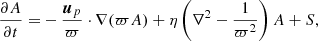 (1)
(1)
![Mathematical equation: $$ \begin{aligned} \frac{\partial B}{\partial t}=&-\varpi \boldsymbol{u}_p\cdot \nabla \left(\frac{B}{\varpi }\right)+\eta \left(\nabla ^2-\frac{1}{\varpi ^2}\right)B+\frac{1}{\varpi }\frac{\partial (\varpi B)}{\partial r}\frac{\mathrm{d}\eta }{\mathrm{d}r}\nonumber \\&-B\nabla \cdot \boldsymbol{u}_p+\varpi [\nabla \times (A\boldsymbol{\hat{e}}_{\phi })]\cdot \nabla \Omega -L, \end{aligned} $$](/articles/aa/full_html/2025/01/aa50968-24/aa50968-24-eq2.gif) (2)
(2)
where ϖ = rsinθ. The effective meridional velocity up = um + γ is the sum of the meridional flow um and turbulent pumping γ, Ω is the local rotation rate (including differential rotation), η is the turbulent diffusivity, and S and L are the BL source and loss terms, respectively. A feature of our model is the inclusion of this toroidal field loss term; it is associated with the emergence of active regions, which give rise to the BL mechanism. Such a loss term was taken into account in the original model of Leighton (1969), but it was quickly abandoned as it was deemed not to be of significance to the magnetic budget of the Sun. However, this assumption was recently shown to be wrong by Cameron & Schüssler (2020), as they determined the corresponding timescale to be commensurate with the 11-year solar cycle. This observational result was further found to be naturally reproduced with the linear loss term of Paper I.
2.2. Differential rotation and meridional circulation
For the differential rotation profile we used the helioseismic measurement of Larson & Schou (2018) taken from data collected by the Helioseismic and Magnetic Imager (HMI), shown here in the left panel of Fig. 1. We did not apply any sort of mask to the profile to ‘correct’ for the high latitudes (e.g. Muñoz-Jaramillo et al. 2009), although the exact rotation rate at these latitudes is rather important (Paper I).
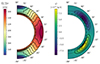 |
Fig. 1. The rotation profile of Larson & Schou (2018) obtained from HMI data (left) and the cycle-averaged and symmetrized stream function of the helioseismic meridional flow inversions of Gizon et al. (2020, right). For the latter, positive values represent clockwise circulation and negative anticlockwise. The dash-dotted and dotted lines represent the approximate locations of the tachocline at 0.7 R⊙ and the reversal of the meridional flow direction at 0.8 R⊙, respectively. |
The meridional flow profile we used is the same as in Paper I and is shown in the right panel of Fig. 1. We constructed it from the helioseismic inversions of Gizon et al. (2020) by symmetrizing the profiles of cycles 23 and 24 across the equator and averaging them.
2.3. Parameterization of turbulent effects
The turbulent parameterizations are the same as in Paper I (see also the references therein). The turbulent diffusivity profile is expressed as
![Mathematical equation: $$ \begin{aligned} \begin{aligned} \eta (r)=&\eta _{\mathrm{RZ} }+\frac{\eta _{\mathrm{CZ} }-\eta _{\mathrm{RZ} }}{2}\left[1+\mathrm{erf} \left(\frac{r-0.72\,R_\odot }{0.012\,R_\odot }\right)\right]\\&+\frac{\eta _{R_\odot }-\eta _{\mathrm{CZ} }-\eta _{\mathrm{RZ} }}{2} \left[1+\mathrm{erf} \left(\frac{r-0.95\,R_\odot }{0.01\,R_\odot }\right)\right], \end{aligned} \end{aligned} $$](/articles/aa/full_html/2025/01/aa50968-24/aa50968-24-eq3.gif) (3)
(3)
where ηRZ = 0.1 km2/s, η R⊙ = 350 km2/s and ηCZ are respectively the radiative core, surface, and bulk values of the turbulent diffusivity. It was found in Paper I that, in this class of models, bulk diffusivities significantly larger than 10 km2/s are not possible because the large radial shear of the observed deep meridional flow gives rise to an effective diffusivity as high as ≃150 km2/s. For most of the models presented in this paper, the value of ηCZ is thus fixed at 10 km2/s. It will, however, be shown that the bulk diffusivity can be significantly increased in the non-linear models, particularly those invoking magnetic buoyancy.
For turbulent pumping we again used the following single step profile:
![Mathematical equation: $$ \begin{aligned} \boldsymbol{\gamma }=-\frac{\gamma _0}{2}\left[1+\mathrm{erf} \left(\frac{r-r_{\gamma }}{0.01\,R_\odot }\right)\right]\boldsymbol{\hat{e}}_r, \end{aligned} $$](/articles/aa/full_html/2025/01/aa50968-24/aa50968-24-eq4.gif) (4)
(4)
where rγ = 0.785 R⊙ corresponds to the depth at mid-latitudes where the meridional flow changes direction (cf. Fig. 1). The toroidal field is in our models essentially stored below that depth (see Paper I for a discussion).
2.4. BL source and loss terms
The BL source and loss terms are given as
 (5)
(5)
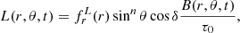 (6)
(6)
where
![Mathematical equation: $$ \begin{aligned} f_r^S(r)&=\frac{1}{2}\left[1+\mathrm{erf} \left(\frac{r-0.85\,R_\odot }{0.01\,R_\odot }\right)\right],\end{aligned} $$](/articles/aa/full_html/2025/01/aa50968-24/aa50968-24-eq7.gif) (7)
(7)
![Mathematical equation: $$ \begin{aligned} f_r^L(r)&=\frac{1}{2}\left[1+\mathrm{erf} \left(\frac{r-0.70\,R_\odot }{0.01\,R_\odot }\right)\right], \end{aligned} $$](/articles/aa/full_html/2025/01/aa50968-24/aa50968-24-eq8.gif) (8)
(8)
and b is the toroidal flux density inside the convection zone:
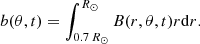 (9)
(9)
Except for the exponent n in the sinnθ terms, these expressions are the same as in Paper I and their derivation can be found there.
The source term above (S) is that of the ϕ-component of the poloidal vector potential A. But the more physically transparent quantity is the radial field generation rate at the surface (Cloutier et al. 2024, hereafter Paper II; see also Appendix A), which from the definition of A (Eq. (1) of Paper I) is readily found to be
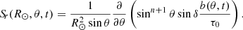 (10)
(10)
Regularity of the source term at the poles is ensured as long as n ≥ 1 (see the second form of Eq. (A.1)).
2.4.1. Latitudinal emergence probability
The sinnθ terms allow us to study cases where emergence at low latitudes is explicitly imposed (Karak & Cameron 2016). In the first set of models, we varied the value of n from 1 to 12. The resulting models are linear, and we chose the values of τ0 and γ0 such that they are critical with a period of 12 years (the average period of cycles 23 and 24). The linearity of the models also means that the fields can be arbitrarily scaled. We normalized the fields so that the maximum net toroidal flux in one hemisphere (here the northern) is max(Φ)=5 × 10²³ Mx, where
 (11)
(11)
This value is consistent with the estimates of Cameron & Schüssler (2015).
2.4.2. Two-regime threshold
In the second set of models the value of n was fixed to 1, representing an emergence probability constant per unit length of toroidal field lines. But we set a threshold, Bthresh, for the average toroidal field,  , between two emergence regimes, τ0slow and τ0fast. This second emergence rate model is based on the observed toroidal field maps which show much higher values of surface Bϕ when active regions begin to emerge, suggestive of a switch between slow and rapid emergence once some threshold is met (see also Cameron & Jiang 2019; Biswas et al. 2022).
We defined the average toroidal field for this purpose as
 (12)
(12)
where we made the approximation that the toroidal field is stored uniformly in the lower half of the convection zone. Then, we introduced a threshold on  , which is equivalent to that on b,
 (13)
(13)
and used it to determine whether flux emergence should be fast or slow:
 (14)
(14)
This threshold prescription makes the model non-linear.
2.4.3. Magnetic buoyancy
Parker (1955) and Jensen (1955) independently showed that magnetic flux tubes initially in thermal equilibrium are buoyant. When they are solely resisted by aerodynamic drag, such flux tubes will float to the surface with terminal rise velocities of the order of the Alfvén velocity (Parker 1975),
 (15)
(15)
 and vc being respectively the Alfvén velocity and the convective velocity given by mixing-length theory (MLT; Prandtl 1925; Vitense 1953; Böhm-Vitense 1958), and
  the equipartition field strength. Taking into account viscous drag and assuming the turbulent viscosity to be given by MLT, the terminal rise velocity of the flux tube is instead of the order of Unno & Ribes (1976)
 (16)
(16)
It should be noted that for both cases the relevant magnetic field, B, is that of the total field.
Kichatinov & Pipin (1993), however, argued that one should instead consider magnetic buoyancy within the framework of mean-field electrodynamics (Moffatt 1978; Krause & Rädler 1980). Employing the second-order correlation approximation, the authors found the same buoyant velocity dependence on  as that found by Unno & Ribes (1976), but with a quenching term due to magnetic tension. For strong mean toroidal fields the rise velocity decreases as
  . In taking into account magnetic buoyancy in our model, we consider both rise velocities, given by Eqs. (15) and (16). For simplicity, we did not consider any effect due to magnetic tension.
Given the implicit condition behind our source and loss terms, that there is a continuous emergence of sunspots over timescales over which the configuration of the mean field changes appreciably (see Paper I), the emergence rate should be proportional to a representative buoyant terminal rise velocity inside the convection zone. Hence, under these assumptions, the timescale parameter is
 (17)
(17)
where τ0b is now the free parameter. The above prescriptions of Parker (1975) and Unno & Ribes (1976) are given by m = 1 and m = 2, respectively. For m > 0 the source and loss terms become non-linear in the magnetic field and thus can, in principle, provide a saturation mechanism for the dynamo. Because we expect the toroidal field to be concentrated at low latitudes, this prescription should not be too dissimilar to the two-regime threshold.
This idea was, in essence, first proposed by Stix (1972) in the context of a non-linear turbulent αΩ dynamo model. Non-linear toroidal field loss due to magnetic buoyancy is not a new feature of αΩ dynamo models (e.g. Schmitt & Schüssler 1989; Moss et al. 1990a,b; Jennings & Weiss 1991). However, our BL source and loss terms are linked (see Paper I), and so magnetic buoyancy must be taken into account in the source term as well. Jouve et al. (2010) and Fournier et al. (2018) have explored the effect of an emergence delay dependent on the magnetic energy of the toroidal field at the bottom of the convection zone, while Karak & Miesch (2017) considered a varying emergence rate, but for 3D models already including tilt quenching and neglecting emergence loss.
3. Observational constraints
3.1. Sunspot number proxy
Flux emergence both removes toroidal magnetic flux from the solar interior and creates poloidal field (and sunspots) at the solar surface. The number of sunspots formed at the surface can be estimated from the amount of toroidal magnetic flux that is lost in the process. We note that typical active regions sizes are around dAR = 100 Mm. Hence, the rate at which flux is generated in active regions is
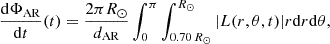 (18)
(18)
where L is the BL loss term defined by Eq. (6). We then divided this quantity by a representative value of the flux contained in a sunspot, which we took to be ΦS = 1021 Mx, so that we have a number of sunspots per year being generated. Assuming these sunspots have a lifetime of one month yields our sunspot number proxy:
 (19)
(19)
A quantity we considered is the ratio of the sunspot number at activity minimum to maximum,
 (20)
(20)
It is a measure of the overlap between cycles.
3.2. Equatorward drift of the sunspot zones
An important discovery is that of Waldmeier (1939, 1955), who found that the equatorward migration of the central heliographic latitude of the sunspot zones, λc, is alike for all cycles, regardless of cycle strength of phase. Indeed, choosing the reference times of individual cycles to be the times of the first appearance of sunspots belonging to those particular cycles (Waldmeier 1935), rather than the times of activity minimum or maximum, the λc-curves superpose; the equatorward drift of the activity belts follows a standard path. This feature was further confirmed by Hathaway (2011, hereafter H11). Employing a parametric function devised by Hathaway et al. (1994) to fit the monthly sunspot number of individual cycles, H11 could determine the start times of cycles 12 to 23 and rediscover the old finding of Waldmeier (1939, 1955). Moreover, H11 could fit the centroid curves as
 (21)
(21)
where time is defined in months and the centroid latitude is λc.
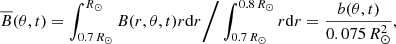
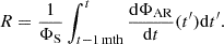
This standard equatorward migration law is an observational constraint on dynamo models. For our models, we assumed the centroid latitude of the sunspot zone, λc, is the latitude where the toroidal flux density, b, is maximum. This latitude closely corresponds to the emergence location of the mean bipolar magnetic region (BMR), as demonstrated in Appendix A and as inferred from the observations (see Fig. 2). Since it is difficult to define exactly when a cycle begins (the functional form for the sunspot number given by H11 may not approximate our sunspot number proxy), we chose the value of t0 so as to obtain the best fit between the centroid latitude curves. As in H11, we find that the start times of our model cycles do not coincide with an activity minimum, here defined as the times where our sunspot proxy, R, is minimum.
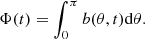
3.3. Polar and butterfly fields
Important observational constraints are the field strengths on the solar surface. However, one must be careful to actually compare the same quantities. The existence of a universal law of sunspot belt migration means that cycles can be averaged together in phase. This fact was pointed out in Paper II, where we further obtained the cycle-averaged butterfly diagram presented in Fig. 2. The mean field strengths of the butterfly wings at cycle maximum, Bb, are around 2 G. Now, because of the open flux problem (Linker et al. 2017), the mean polar field at cycle minima, Bp, could be anywhere in the range of 3−15 G (Petrie 2015, although it is more likely to be on the higher end, if not higher; for more on that, see Sinjan et al. 2024).
3.4. Toroidal flux loss timescale and cycle phase of polar maxima
The toroidal flux loss timescale τ and its contributions due to emergence τL and diffusive τη loss through the surface are as defined in Paper I. We again took their combination to be τ−1 = τL−1 + τη−1. We calculated these timescales at the time when the polar field reverses. The phase difference between the polar field and cycle maxima Δϕ is also defined in Paper I.
4. Results
All the solutions we present are predominantly of dipolar parity, although our model does allow different parities. In terms of the rush to the poles, it has only been observed for the dipole mode. Therefore, we restricted our analysis and discussion to the dipole dynamo mode.
4.1. Models with an explicit preference for emergence at low latitudes
To look into the effect of n on the latitudinal emergence probability, we computed critical linear models (Bthresh = 0 and m = 0) with values of n = 1, 3, 6 and 12 (see Eqs. 5 and 6). The solutions are shown in Figs. 3, 4, and 5, which show the toroidal flux density, b, the surface radial source term, Sr, and the surface radial field, Br, respectively. The location of the maximum toroidal field density is represented by a dashed line.
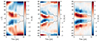 |
Fig. 2. Mean observed butterfly diagram and poloidal field generation rate. Left panel: Cycle-averaged butterfly diagram from Paper II. Middle panel: Surface radial source term obtained from the left panel by ‘inverting’ a 1D SFT model. Right panel: Surface radial source term obtained from the surface toroidal field (not shown) using an emergence model. See Paper II for more information. The dashed lines represent the location of the maximum surface toroidal field. |
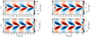 |
Fig. 3. Time-latitude diagrams of the toroidal flux density, b, for different values of n: 1 (upper left), 3 (upper right), 6 (lower left), and 12 (lower right). |
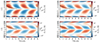 |
Fig. 5. Same as Fig. 3 but for the surface radial field, Br(R⊙). The colour scale is logarithmic to better show the different features. |
The n = 1 case is essentially the same as the reference model of Paper I, the only difference being the differential rotation profile. The lack of a distinct rush to the poles in the butterfly diagram is obvious. As expected, increasing the value of n forces emergences to occur at increasingly lower latitudes. A high-latitude rush to the poles becomes noticeable at around 60° near cycle maximum for the n = 3 case. By n = 12, the rush starts at about 30°. The presence of a rush to the poles is not a necessary consequence of the toroidal field being mostly stored below 30°. In fact, as it can be appreciated in Fig. 3, the toroidal field is more confined to low latitudes in the n = 1 case. Especially in the n = 12 case, there is strong toroidal field at the poles and significant field strengths at mid-latitudes. This is because larger values of n cause more cross-equator poloidal flux cancellation and hence stronger polar fields. The radial shear present throughout the whole depth of the polar convection zone then generates this high-latitude toroidal field. The pumping required to obtain critical 12-year periodic solutions also decreases with increasing n, causing more poloidal field to reach the poles. As discussed in Paper I, stronger pumping is required in the n = 1 case to concentrate the toroidal field at low latitudes, ensuring dynamo action. This is not necessary when n > 1 as high latitude emergences are then inhibited.
Figure 4 shows the poloidal field generation rate of the models, which must be compared to the observationally inferred one presented in Paper II and shown in Fig. 2. As in Paper II, we clearly see two large regions where a mean poloidal field of opposite polarities is being generated at each timestep. The lack of a rush to the poles in the n = 1 case is due to the emergence of flux at all latitudes; even though the toroidal field is concentrated near the equator, there is still enough emergence happening at higher latitudes to prevent the appearance of a rush to the poles. The trailing spot fields migrating polewards from say 30° are weak, being spread out over about 60° in latitude, and so the much stronger leading spot fields emerging at low latitude emergences dominate over them at mid-latitudes. In other words, what we see at mid-latitudes is the poleward migration of the leading polarity field. Increasing n reduces the high-latitude emergence rate and hence allows the trailing polarity flux to be advected towards the poles and therefore to dominate at mid-latitudes and above.
Figure 6 compares the observed rate of the equatorial drift of sunspot zones (Eq. (21)) with that of the toroidal flux system for the models discussed above. The model with n = 1 matches the observed equatorial drift well, with models with other n matching less well.
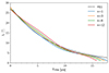 |
Fig. 6. Comparison of the H11 standard law of sunspot zone migration with that obtained by linear models. |
4.2. Models with either slow or fast emergence based on the toroidal flux density
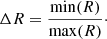
In this section we show a selection of models incorporating the two-regime threshold described in Sect. 2.4.2. We computed grids of models with different values of τ0 and γ0 for two values of the threshold field, Bthresh = 1 kG and 1.35 kG, and bulk diffusivity, ηCZ = 10 and 20 km2/s. We present four of the models that best fit a number of observational constraints: the surface radial field inside the butterfly wings of ∼5 G, polar fields that are not too strong, a cycle period reasonably close to 12 years, and little flux emergence in the polar regions. The four solutions are presented in Figs. 7, 8, 9, and 10, which we respectively call Models TA, TB, TC, and TD. The parameter values are found in Table 1. The different output quantities are presented in Table 2.
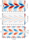 |
Fig. 7. Time-latitude diagrams of the toroidal flux density, b (top), the surface radial source term, Sr(R⊙) (middle), and the surface radial field, Br(R⊙) (bottom) for Model TA. |
Input parameters of the threshold models.
Output quantities of the threshold models.
All models now present a clear, strong, initial rush to the poles. This is followed by a weak poleward surge of leading polarity near activity maximum, followed by more trailing polar flux until the cycle ends.
The source term shows strong poloidal flux production at the edges where the threshold condition is met. This is a consequence of the fact that the threshold introduces a discontinuity in S, which is the source term in the equation for A. In the absence of diffusion, the resulting discontinuity in S leads to a delta function in Sr. The presence of diffusion smooths these singular features.
As in Biswas et al. (2022), the presence of a threshold in flux emergence and the flux depletion associated with it causes the dynamo to saturate. Because it is the amount of leading poloidal flux cancelling across the equator that determines the strength of the Sun’s dipole, emergences at high latitudes are inefficient at generating polar fields (Jiang et al. 2014). As stronger cycles present emergences at higher latitudes than weaker ones, the polar field at cycle minimum is weaker and consequently so is the subsequent cycle. This saturation mechanism is known as latitudinal quenching (Jiang 2020; Karak 2020; Talafha et al. 2022). For the particular model parameters chosen here, latitudinal quenching, by itself, is not sufficient to saturate the dynamo. The addition of emergence loss causes the early, high-latitude emergences of stronger cycles to deplete the sub-surface toroidal flux reservoir very quickly, enhancing the effect of latitudinal quenching. We note that the observational results of Waldmeier are seen as evidence of latitudinal quenching in the solar dynamo (Waldmeier 1955; Cameron & Schüssler 2023). As explained by Biswas et al. (2022), the non-linearity involving emergence loss and the threshold makes the decline phase independent of cycle strength.
We briefly explored the effects of varying the model parameters. Decreasing τ0fast causes a narrowing of the butterfly wings (compare Figs. 8 and 10), while increasing γ0 causes not only a widening of the butterfly wings, but a stronger one during the ascending phase of the cycle. Increasing ηCZ makes the period longer and necessitates a significant increase in pumping. Bthresh essentially sets the normalization of the magnetic field. Models with values of Bthresh much larger than 1 kG have fields much too strong compared to observations. This value of Bthresh is significantly weaker than the equipartition value of 5 − 6 kG as inferred from MLT (although it is in practice likely quenched by rotation and magnetic fields).
Figure 11 compares the H11 law with the equatorward migration of the toroidal flux system of threshold models. All models reproduce the observed behaviour reasonably well.
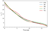 |
Fig. 11. Comparison of the H11 standard law of sunspot zone migration with that obtained by threshold models. |
4.3. Models where the emergence rate is based on magnetic buoyancy
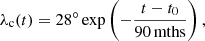
In this section we show a selection of models incorporating magnetic buoyancy in the source and loss terms, as described in Sect. 2.4.3. Contrary to Sect. 4.2, all the models we present have the same values of τ0b = 72 yr and γ0 = 30 m/s. The model that best reproduce the observations with a ‘reasonable’ pumping amplitude will be our ‘reference model’, with m = 2 and ηCZ = 35 km2/s (model BA). We then changed a few parameters individually to study their effect on the solution; the loss term switched off L = 0 (model BB), a weaker diffusivity ηCZ = 10 km2/s (model BC), and the emergence rate proportional to the toroidal field strength m = 1 (model BD – here a lower diffusivity is necessary). They are presented in Figs. 12–15. Two additional models, which do not present sufficiently different time-latitude diagrams to be shown, have been computed. They are Model BE having a pumping amplitude of γ0 = 100 m/s and Model BF using the meridional flow profile of cycle 23. At mid-latitudes at the bottom of the convection zone, the amplitude of the meridional flow is 4.8 m/s for cycle 23 and 3.6 m/s for cycle 24, meaning that in model BF this velocity is increased from their average by 0.6 m/s. The input parameters and output quantities are presented in Tables 3 and 4, respectively.
Input parameters of the magnetic buoyancy models.
Output quantities of the magnetic buoyancy models.
Model BA is, out of all the models presented in this paper, the most solar-like. It reproduces a clear rush to the poles without any opposite polarity surge. The width of the butterfly wings is somewhat below 30°, which is in good agreement with what is found in Paper II for the observed mean butterfly diagram (see also Fig. 2), and is only weakly dependent on the model parameters. With Bb = 2 G, the field strength inside the butterfly wings is consistent with that of the observed mean butterfly diagram of Paper II (see Fig. 2). With Bp = 14.2 G, the polar field strengths are also consistent with observations. The maximal value of the net toroidal flux in one hemisphere is max(Φ)=5.3 × 10²³ Mx, which is in good agreement with the estimates of Cameron & Schüssler (2015). The phase difference between the poloidal and toroidal fields, however, remains large at Δϕ = 138°. This could be due to our models being close to symmetric with respect to cycle maximum. A faster rising phase would imply a stronger rush to the poles, reversing the polar field more quickly. The cycle period is also rather long at 14.6 yr. It is possible to decrease the cycle period by either increasing turbulent pumping or decreasing the diffusivity. The latter makes the model less solar-like (see Fig. 14), while the former requires excessively strong pumping velocities to significantly lower the cycle period. The cycle period is independent of the value of τ0b. This is because τ0b combines with beq, which acts to normalize the magnetic field strength. The value of τ0b was chosen so that Bb = 2 G. The emergence loss timescale is also constant during the declining phases at τL = 32.4 yr, where τη ≃ 180 yr so that τ ≃ 27 yr. This is very close to the magnetic period of 29.2 years, and only a factor of 2 larger than the rough 12-year estimate of Cameron & Schüssler (2020).
To investigate the effect of the loss term on the solutions, we computed Model BB (Fig. 13) where the loss term has been turned off. Unlike for the threshold prescription, the dynamo still saturates. A more precise look into the saturation of the buoyancy dynamo is presented in Appendix A. Switching off the loss term also leads to a shorter period, a full 5 years shorter (compare with Paper I). Emergence loss could therefore play an important role in setting the cycle period.
Model BC (Fig. 14) has a lower value of the bulk diffusivity. The activity period is significantly decreased and is now only 10.7 years. Increasing the diffusivity, like turning on the loss term, spreads out the sub-surface toroidal field, slowing its buildup near the equator. Weaker diffusivity also makes the emergence loss timescale τL much closer to the activity period (because the early strong emergences deplete the toroidal flux very quickly), and the total toroidal flux loss timescale τ slightly below it.
We also tested the effect of the value of m for the non-linearity and computed Model BD (Fig. 15) where m = 1. The butterfly wings are slightly wider than those of Model BC because of the decreased non-linearity. Interestingly, all output quantities of Model BD in Table 4 are very close to those of Model BC, which is the same save for a value of m = 2, except for the quantities depending on the amplitude of the magnetic field. For those, they are a bit more than a factor of 2 larger, so that decreasing τ0b can bring them in relatively good agreement. Consequently, the degree of non-linearity has a weak effect on the solutions.
Increasing the turbulent pumping amplitude by more than a factor of 3 (Model BE) decreases the period by only 1.3 years. At a large value of 30 m/s, the time required for the magnetic field to reach the lower convection zone is already relatively close to instantaneous with respect to the cycle period.
Using instead the meridional flow profile of cycle 23 (Model BF), the period is decreased by a full 2.5 years, illustrating the key role of the meridional flow on setting the cycle period. A faster meridional flow also significantly decreases the emergence loss timescale compared to the activity period. This is because by compressing the toroidal field closer to the equator, a faster meridional flow allows for stronger emergences to deplete the sub-surface toroidal field more quickly. We comment here that the flow amplitudes at the bottom of the convection zone for cycles 23 and 24 are both within the error bars of the helioseismic inversions of Gizon et al. (2020), despite the resulting periods differing by 2.5 years.
Comparing Figs. 2 and 12, we see that the agreement between our buoyancy model and observations is remarkable. The shape of the butterfly wings and their width is very well reproduced. But the model surface radial source term is also very similar to the observed one (obtained by ‘inverting’ a 1D SFT model with the observed butterfly diagram – middle panel of Fig. 2). Even the location of maximum toroidal field (corrected for the low resolution) is in agreement.
In Fig. 16 we compare the equatorial migration of the toroidal flux of our buoyancy models with the observed sunspot belt migration. For models BA to BD, the equatorial drift in the model is substantially faster than what is observed (consistent with the cycles being shorter). The match with observations is improved if the pumping is strongly increased to 100 m/s (Model BE). For Model BF with a faster meridional flow, the agreement is even better and remarkably good. The slowdown of the drift of the sunspot zones compared to Eq. (21) about midway into the declining phase seen for models BA, BE, and BF is a feature also appearing in the observations (cf. Fig. 5 of H11 and Fig. 2 of Paper II).
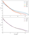 |
Fig. 16. Comparison of the H11 standard law of sunspot zone migration with that obtained by buoyancy models. |
The bulk turbulent diffusivity of 35 km2/s used in our buoyancy models is about a factor of 30 lower than MLT estimates, ∼1000 km2/s (e.g. Muñoz-Jaramillo et al. 2011). In principle, magnetic diffusivity can be significantly quenched both by rotation and the magnetic field (Kitchatinov et al. 1994; Featherstone & Hindman 2016; Hotta & Kusano 2021, see Cloutier 2024 for a discussion on the matter). Furthermore, the corresponding MLT convective length scale is that of the giant cells, which seem to be ruled out by observations (Hanasoge et al. 2012; Gizon et al. 2021). Mean-field theory predicts turbulent diffusivity to be given by  (e.g. Krause & Rädler 1980), where τc is the convective correlation time. Its value can be estimated from helioseismology or local correlation tracking. With values of vc ≃ 10 m/s and τc ≃ 1 month (Hathaway & Upton 2021), η ≃ 86 km2/s. This is around a factor of 2 larger than the value used in our buoyancy models, but is a factor of 10 smaller than the MLT estimate. Lastly, we mention again the possible role of the helioseismically inferred meridional flow in contributing to most of the total diffusivity in our models (Sect. 2.3).
5. Conclusion
The goal of this study was to identify mechanisms by which the rush to the poles could be reproduced in BL-FTD models. A mechanism either suppressing emergences at high latitudes or enhancing emergences at low latitudes is necessary, even if the toroidal field is weak close to the poles and mostly stored near the equator. An emergence probability quickly decreasing with latitude is one such mechanism. The physical reason in this case would be related to the latitudinal dependence of the growth rate of the instability giving rise to the emergence of flux tubes. Alternatively, non-linear mechanisms, such as a threshold for flux emergence and an emergence rate based on magnetic buoyancy, not only help reproduce the rush to the poles but provide a saturation mechanism for the dynamo. They produce latitudinal quenching. Latitudinal quenching is believed to be related to the solar cycle property that all cycles decline the same way (Cameron & Schüssler 2023).
The ‘best-fit’ model butterfly diagrams making use of the buoyancy prescription (Fig. 12) is strikingly similar to the mean observed one (Fig. 2), as are the poloidal field generation rates. The width of the butterfly wings is found to be only weakly dependent on model parameters and is ≲ ± 30°, in good agreement with observations. It is the saturation of the dynamo that controls this width. Moreover, the equatorward drift of the activity belts is found to be in good agreement with that inferred from observations, implying the toroidal field could be stored at equatorial latitudes deep in the convection zone.
An interesting finding of this paper is just how much the depletion of toroidal flux deep in the convection zone leading to the emergence of poloidal flux at the surface lengthens the cycle period for non-linear models. It can be slowed by as much as ≃60%, with the timescale associated with the toroidal flux loss through the surface being comparable to the magnetic period. What sets the cycle period could hence diverge from the usual dynamo-wave-FTD dichotomy, with emergence loss possibly playing an important role.
We stress that our model incorporates the observed axisymmetric flows (differential rotation and meridional circulation). For this reason, our model cannot be easily used to draw inferences about the dynamos of other stars. At the very least, an extension that models the differential rotation and meridional circulation of other stars would be necessary.
Acknowledgments
The authors wish to thank the anonymous referee for comments that helped improve the overall quality of this paper. This work was carried out when SC was a member of the International Max Planck Research School for Solar System Science at the University of Göttingen. The authors acknowledge partial support from ERC Synergy grant WHOLE SUN 810218.
References
- Altrock, R. C. 1997, Sol. Phys., 170, 411 [NASA ADS] [CrossRef] [Google Scholar]
- Ananthakrishnan, R. 1954, Proc. Indian Acad. Sci. Sect. A, 40, 72 [Google Scholar]
- Biswas, A., Karak, B. B., & Cameron, R. 2022, Phys. Rev. Lett., 129, 241102 [Google Scholar]
- Böhm-Vitense, E. 1958, Z. Astrophys., 46, 108 [Google Scholar]
- Cameron, R. H., & Jiang, J. 2019, A&A, 631, A27 [NASA ADS] [CrossRef] [EDP Sciences] [Google Scholar]
- Cameron, R., & Schüssler, M. 2015, Science, 347, 1333 [Google Scholar]
- Cameron, R. H., & Schüssler, M. 2020, A&A, 636, A7 [NASA ADS] [CrossRef] [EDP Sciences] [Google Scholar]
- Cameron, R. H., & Schüssler, M. 2023, Space Sci. Rev., 219, 60 [NASA ADS] [CrossRef] [Google Scholar]
- Charbonneau, P. 2014, ARA&A, 52, 251 [NASA ADS] [CrossRef] [Google Scholar]
- Cloutier, S. 2024, Ph.D. Thesis, Georg-August-Universität Göttingen, Germany [Google Scholar]
- Cloutier, S., Cameron, R. H., & Gizon, L. 2023, A&A, 680, A42 [NASA ADS] [CrossRef] [EDP Sciences] [Google Scholar]
- Cloutier, S., Cameron, R. H., & Gizon, L. 2024, A&A, 691, A9 [NASA ADS] [CrossRef] [EDP Sciences] [Google Scholar]
- Featherstone, N. A., & Hindman, B. W. 2016, ApJ, 830, L15 [Google Scholar]
- Fournier, Y., Arlt, R., & Elstner, D. 2018, A&A, 620, A135 [NASA ADS] [CrossRef] [EDP Sciences] [Google Scholar]
- Gizon, L., Cameron, R. H., Pourabdian, M., et al. 2020, Science, 368, 1469 [Google Scholar]
- Gizon, L., Cameron, R. H., Bekki, Y., et al. 2021, A&A, 652, L6 [NASA ADS] [CrossRef] [EDP Sciences] [Google Scholar]
- Hanasoge, S. M., Duvall, T. L., & Sreenivasan, K. R. 2012, Proc. Natl. Acad. Sci., 109, 11928 [Google Scholar]
- Hathaway, D. H. 2011, Sol. Phys., 273, 221 [NASA ADS] [CrossRef] [Google Scholar]
- Hathaway, D. H., & Upton, L. A. 2021, ApJ, 908, 160 [NASA ADS] [CrossRef] [Google Scholar]
- Hathaway, D. H., Wilson, R. M., & Reichmann, E. J. 1994, Sol. Phys., 151, 177 [NASA ADS] [CrossRef] [Google Scholar]
- Hotta, H., & Kusano, K. 2021, Nat. Astron., 5, 1100 [NASA ADS] [CrossRef] [Google Scholar]
- Jennings, R. L., & Weiss, N. O. 1991, MNRAS, 252, 249 [Google Scholar]
- Jensen, E. 1955, Ann. Astrophys., 18, 127 [NASA ADS] [Google Scholar]
- Jiang, J. 2020, ApJ, 900, 19 [Google Scholar]
- Jiang, J., Cameron, R. H., & Schüssler, M. 2014, ApJ, 791, 5 [Google Scholar]
- Jouve, L., Proctor, M. R. E., & Lesur, G. 2010, A&A, 519, A68 [CrossRef] [EDP Sciences] [Google Scholar]
- Karak, B. B. 2020, ApJ, 901, L35 [NASA ADS] [CrossRef] [Google Scholar]
- Karak, B. B., & Cameron, R. 2016, ApJ, 832, 94 [NASA ADS] [CrossRef] [Google Scholar]
- Karak, B. B., & Miesch, M. 2017, ApJ, 847, 69 [NASA ADS] [CrossRef] [Google Scholar]
- Kitchatinov, L. L. 2020, ApJ, 893, 131 [NASA ADS] [CrossRef] [Google Scholar]
- Kichatinov, L. L., & Pipin, V. V. 1993, A&A, 274, 647 [NASA ADS] [Google Scholar]
- Kitchatinov, L. L., Pipin, V. V., & Ruediger, G. 1994, Astron. Nachr., 315, 157 [NASA ADS] [CrossRef] [Google Scholar]
- Krause, F., & Rädler, K. H. 1980, Mean-field Magnetohydrodynamics and Dynamo Theory (Oxford: Pergamon Press) [Google Scholar]
- Larson, T. P., & Schou, J. 2018, Sol. Phys., 293, 29 [Google Scholar]
- Leighton, R. B. 1969, ApJ, 156, 1 [Google Scholar]
- Linker, J. A., Caplan, R. M., Downs, C., et al. 2017, ApJ, 848, 70 [NASA ADS] [CrossRef] [Google Scholar]
- Moffatt, H. K. 1978, Magnetic Field Generation in Electrically Conducting Fluids (Cambridge: Cambridge University Press) [Google Scholar]
- Moss, D., Tuominen, I., & Brandenburg, A. 1990a, A&A, 228, 284 [NASA ADS] [Google Scholar]
- Moss, D., Tuominen, I., & Brandenburg, A. 1990b, A&A, 240, 142 [NASA ADS] [Google Scholar]
- Muñoz-Jaramillo, A., Nandy, D., & Martens, P. C. H. 2009, ApJ, 698, 461 [CrossRef] [Google Scholar]
- Muñoz-Jaramillo, A., Nandy, D., & Martens, P. C. H. 2011, ApJ, 727, L23 [NASA ADS] [CrossRef] [Google Scholar]
- Parker, E. N. 1955, ApJ, 121, 491 [Google Scholar]
- Parker, E. N. 1975, ApJ, 198, 205 [NASA ADS] [CrossRef] [Google Scholar]
- Petrie, G. J. D. 2015, Liv. Rev. Sol. Phys., 12, 5 [Google Scholar]
- Prandtl, L. 1925, Zeitschrift für Angewandte Mathematik und Mechanik, 5, 136 [Google Scholar]
- Schmitt, D., & Schüssler, M. 1989, A&A, 223, 343 [NASA ADS] [Google Scholar]
- Sinjan, J., Solanki, S. K., Hirzberger, J., Riethmüller, T. L., & Przybylski, D. 2024, A&A, 690, A341 [NASA ADS] [CrossRef] [EDP Sciences] [Google Scholar]
- Stix, M. 1972, A&A, 20, 9 [NASA ADS] [Google Scholar]
- Talafha, M., Nagy, M., Lemerle, A., & Petrovay, K. 2022, A&A, 660, A92 [NASA ADS] [CrossRef] [EDP Sciences] [Google Scholar]
- Unno, W., & Ribes, E. 1976, ApJ, 208, 222 [NASA ADS] [CrossRef] [Google Scholar]
- Vitense, E. 1953, Z. Astrophys., 32, 135 [NASA ADS] [Google Scholar]
- Waldmeier, M. 1935, Astronomische Mitteilungen der Eidgenössischen Sternwarte Zürich, 14, 105 [Google Scholar]
- Waldmeier, M. 1939, Astronomische Mitteilungen der Eidgenössischen Sternwarte Zürich, 14, 470 [Google Scholar]
- Waldmeier, M. 1955, Ergebnisse und Probleme der Sonnenforschung (Leipzig: Akademische Verlagsgesellschaft Geest& Portig) [Google Scholar]
- Yeates, A. R., Cheung, M. C. M., Jiang, J., Petrovay, K., & Wang, Y.-M. 2023, Space Sci. Rev., 219, 31 [CrossRef] [Google Scholar]
Appendix A: Saturation of the buoyancy dynamo
That our models with the buoyancy prescription (m > 0) saturate even with the loss term turned off, means that the latitudinal quenching of the buoyancy dynamo is much stronger than that of the threshold dynamo. To shed light on this matter, it is advantageous to look not into the usual source term for the ϕ-component of the poloidal vector potential A (Eq. (5)), but into the source term for the radial field at the surface (Eq. (10)). It can be rewritten as
 (A.1)
(A.1)
where
 (A.2)
(A.2)
By introducing the polarity function p, which determines the polarity of the radial field being generated, Sr can be rewritten in a way formally similar to S (second equality). The minus sign was chosen so that for p(θ, t)> 0 the polarity being generated is that of the leading spot (in the northern hemisphere).
Setting p = 0 yields the latitude where the switch in polarity of the average BMR occurs, in other words the location of the centre of the mean BMR being generated. We thus have a condition on the maximal value of ∂lnb/∂θ for leading spot polarity to be generated:
 (A.3)
(A.3)
where  (Leighton 1969). This condition is shown in Fig. A.1 (blue and green lines). As we go equatorwards from the poles, ∂lnb/∂θ is positive and maximal close to the edge of the low-latitude toroidal flux concentration, zero where this concentration is at its maximum, and negative very close to the equator. Wherever the maximal b-gradient is negative, trailing polarity is generated. The latitude where this gradient is zero (i.e. where the toroidal flux density, b, is maximum) constitutes a lower bound on the latitude of the mean BMR centre.
 |
Fig. A.1. Maximal value of ∂lnb/∂θ possible for the generation of leading polarity field at latitude λ for values of n = 1, 3, 6, 12 (solid, dash-dotted, dashed and dotted lines respectively). Blue, green and red lines represent cases where m = 0, m = 2 and constant tilt angle. |
Not unexpectedly, forcing emergences to occur at lower latitudes by increasing the value of n shifts this mean BMR towards the equator. One of the consequences is to increase the polar field strength, as cross-equatorward flux cancellation of the leading spot fields is increased. Increasing the non-linearity in the b of the source term (i.e. increasing the value of m) decreases the maximal b-gradient so that the centre of the mean BMR is also shifted equatorwards.
If Joy’s law were to be constant with latitude (Fig. A.1, red lines), leading spot polarity would be produced only very close to the equator, after the maximum of b. If the average leading spot was to be produced so close to the equator, most of the leading flux would diffusively cancel across the equator and the resulting polar field would be extremely large, not to mention that the butterfly diagram would look very different from the observations. The exact form of Joy’s law thus largely sets what the butterfly diagram looks like.
Examining Eqs. (A.1) and (A.2), we see that increasing the toroidal flux density b does not shift the centre of the mean BMR. Taking the derivative of the second form of Eq. (A.1) with respect to b yields
 (A.4)
(A.4)
Increasing b everywhere by the same factor causes a linear or non-linear increase in the radial source term (rather than a uniform increase) in such a way that the largest increase occurs near the mean BMR centre. The field is thus redistributed closer to the centre such that more intra-hemisphere flux cancellation occurs and the polar field is weakened; this constitutes a saturation mechanism. There is here an analogy with tilt quenching. It is as if the tilt of the mean BMR was decreased, leading to less cross-equator flux cancellation. This is, of course, not true tilt quenching, as the tilt of the individual emergences is constant in our models. The emergence rate simply changes as a function of latitude in such a way that the mean BMR’s tilt appears smaller.
But this is not the entire picture. While a proportional increase in b does not change the location of the mean BMR being generated, the non-linearity of the BL source term leaves an imprint on the Ω-effect and the toroidal field it induces for the next cycle. The distribution of the sub-surface toroidal field changes as well. If, because of this non-linearity, significant toroidal field strengths are reached at higher latitudes, meaning that we have a stronger cycle with broader sunspot zones, the b-gradient is flattened, causing the mean BMR centre to shift polewards. This, in turn, weakens the polar fields through increased cross-hemispheric flux cancellation of the generated radial field; this corresponds to latitudinal quenching (not only in the sense of the mean BMR). There is thus an interaction between the ‘tilt’ and latitudinal quenchings. They, however, act against each other (as in Karak & Miesch 2017, where there is true tilt quenching). The competition between both saturation mechanisms is what controls the width of the butterfly wings (on that see also Karak 2020, although his model does not incorporate tilt quenching and the latitudinal quenching arises from a latitudinal dependence on the critical field strength required for flux emergence).
All Tables
All Figures
|
Fig. 1. The rotation profile of Larson & Schou (2018) obtained from HMI data (left) and the cycle-averaged and symmetrized stream function of the helioseismic meridional flow inversions of Gizon et al. (2020, right). For the latter, positive values represent clockwise circulation and negative anticlockwise. The dash-dotted and dotted lines represent the approximate locations of the tachocline at 0.7 R⊙ and the reversal of the meridional flow direction at 0.8 R⊙, respectively. |
| In the text | |
|
Fig. 2. Mean observed butterfly diagram and poloidal field generation rate. Left panel: Cycle-averaged butterfly diagram from Paper II. Middle panel: Surface radial source term obtained from the left panel by ‘inverting’ a 1D SFT model. Right panel: Surface radial source term obtained from the surface toroidal field (not shown) using an emergence model. See Paper II for more information. The dashed lines represent the location of the maximum surface toroidal field. |
| In the text | |
|
Fig. 3. Time-latitude diagrams of the toroidal flux density, b, for different values of n: 1 (upper left), 3 (upper right), 6 (lower left), and 12 (lower right). |
| In the text | |
 |
Fig. 4. Same as Fig. 3 but for the surface radial source term, Sr(R⊙). |
| In the text | |
|
Fig. 5. Same as Fig. 3 but for the surface radial field, Br(R⊙). The colour scale is logarithmic to better show the different features. |
| In the text | |
|
Fig. 6. Comparison of the H11 standard law of sunspot zone migration with that obtained by linear models. |
| In the text | |
|
Fig. 7. Time-latitude diagrams of the toroidal flux density, b (top), the surface radial source term, Sr(R⊙) (middle), and the surface radial field, Br(R⊙) (bottom) for Model TA. |
| In the text | |
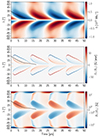 |
Fig. 8. Same as Fig. 7 but for Model TB. |
| In the text | |
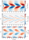 |
Fig. 9. Same as Fig. 7 but for Model TC. |
| In the text | |
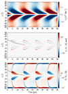 |
Fig. 10. Same as Fig. 7 but for Model TD. |
| In the text | |
|
Fig. 11. Comparison of the H11 standard law of sunspot zone migration with that obtained by threshold models. |
| In the text | |
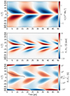 |
Fig. 12. Same as Fig. 7 but for Model BA. |
| In the text | |
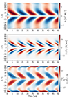 |
Fig. 13. Same as Fig. 7 but for Model BB. |
| In the text | |
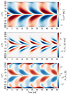 |
Fig. 14. Same as Fig. 7 but for Model BC. |
| In the text | |
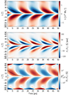 |
Fig. 15. Same as Fig. 7 but for Model BD. |
| In the text | |
|
Fig. 16. Comparison of the H11 standard law of sunspot zone migration with that obtained by buoyancy models. |
| In the text | |
|
Fig. A.1. Maximal value of ∂lnb/∂θ possible for the generation of leading polarity field at latitude λ for values of n = 1, 3, 6, 12 (solid, dash-dotted, dashed and dotted lines respectively). Blue, green and red lines represent cases where m = 0, m = 2 and constant tilt angle. |
| In the text | |
Current usage metrics show cumulative count of Article Views (full-text article views including HTML views, PDF and ePub downloads, according to the available data) and Abstracts Views on Vision4Press platform.
Data correspond to usage on the plateform after 2015. The current usage metrics is available 48-96 hours after online publication and is updated daily on week days.
Initial download of the metrics may take a while.