| Issue |
A&A
Volume 691, November 2024
|
|
|---|---|---|
| Article Number | A9 | |
| Number of page(s) | 5 | |
| Section | The Sun and the Heliosphere | |
| DOI | https://doi.org/10.1051/0004-6361/202450739 | |
| Published online | 25 October 2024 | |
The mean solar butterfly diagram and poloidal field generation rate at the surface of the Sun
1
Max-Planck-Institut für Sonnensystemforschung, Justus-von-Liebig-Weg 3, 37077 Göttingen, Germany
2
Institut für Astrophysik und Geophysik, Georg-August-Universität Göttingen, 37077 Göttingen, Germany
⋆ Corresponding author; This email address is being protected from spambots. You need JavaScript enabled to view it.
Received:
16
May
2024
Accepted:
2
September
2024
Abstract
Context. The difference between individual solar cycles in the magnetic butterfly diagram can mostly be ascribed to the stochasticity of the emergence process.
Aims. We aim to obtain the expectation value of the butterfly diagram from observations of four cycles. This allows us to further determine the generation rate of the surface radial magnetic field.
Methods. We used data from Wilcox Solar Observatory to generate time-latitude diagrams of the surface radial and toroidal magnetic fields spanning cycles 21–24. We symmetrized them across the equator and cycle-averaged them. From the mean butterfly diagram and surface toroidal field, we then inferred the mean poloidal field generation rate at the surface of the Sun.
Results. The averaging procedure removes realization noise from individual cycles. The amount of emerging flux required to account for the evolution of the surface radial field is found to match that provided by the observed surface toroidal field and Joy’s law.
Conclusions. Cycle-averaging butterfly diagrams removes realization noise and artefacts due to imperfect scale separation and corresponds to an ensemble average that can be interpreted in the mean-field framework. The result can then be directly compared to αΩ-type dynamo models. The Babcock-Leighton α-effect is consistent with observations, a result that can be appreciated only if the observational data are averaged in some way.
Key words: Sun: activity / Sun: magnetic fields
© The Authors 2024
 Open Access article, published by EDP Sciences, under the terms of the Creative Commons Attribution License (https://creativecommons.org/licenses/by/4.0), which permits unrestricted use, distribution, and reproduction in any medium, provided the original work is properly cited.
This article is published in open access under the Subscribe to Open model.
Open Access funding provided by Max Planck Society.
1. Introduction
The 11-year solar cycle is believed to be driven by a hydromagnetic dynamo seated somewhere in the convection zone of the Sun (Charbonneau 2020). The dynamo loop consists of two parts: one where toroidal field is generated from the poloidal field, and the other where poloidal field of opposite sign is generated from the new toroidal field. It takes another solar cycle, or half of the magnetic cycle, to revert to the original polarity. The first part is relatively well understood and takes place via the Ω-effect, whereby the poloidal field is wound up in the azimuthal direction by differential rotation, which is observationally well constrained by helioseismology (e.g. Schou et al. 1998). The second part, on the other hand, involves the unobservable subsurface toroidal field and two possible mechanisms: the α-effect (Parker 1955b; Steenbeck et al. 1966) and the Babcock-Leighton (BL) mechanism (Babcock 1961; Leighton 1964, 1969). This dynamo loop is often studied using mean-field models.
The mean field of mean-field electrodynamics is defined in terms of an average that can be spatial, temporal, or ensemble. In the case of the Sun, the azimuthal average is a natural choice. In fact, the butterfly diagram is constructed by longitudinally averaging line-of-sight synoptic magnetograms. The symmetric component (with respect to the solar meridian) is then extracted, from which the radial field is obtained by assuming it is the only component of the poloidal field at the surface. Finally, the butterfly diagram is obtained by stacking the result in time. In principle, butterfly diagrams are thus of a mean-field nature and can be directly compared to models.
A caveat, however, is that scale separation is likely to be poor in the Sun as supergranulation reaches down to about 5% of the solar radius, which is non-negligible with respect to the depth of the convection zone and the scales of differential rotation and the meridional flow. The picture is much worse if we consider active regions (which, by being largely non-axisymmetric, are supposed to be small-scale in nature), with sizes of the order of 100 Mm, or about half the depth of the convection zone. Consequently, the observed butterfly diagram cannot be directly compared to mean-field models. A way to circumvent this problem is by considering different solar cycles as different realizations of the underlying dynamo and ensemble-averaging them; we note that this is not a true ensemble average in the mean-field sense (see Hoyng 2003) but is aimed at reproducing the azimuthal average used in models with reduced realization noise. In other words, averaging different cycles together to remove realization noise (fluctuating dynamo parameters) and the effects of imperfect scale separation.
The way cycles are to be averaged together requires careful consideration. It has been shown that defining cycles in terms of activity minimum or maximum is not ideal (Waldmeier 1935; Hathaway 2011). But when cycles are instead defined according to their start time, they all present the same equatorward pattern of sunspot migration, regardless of strength; the location of the sunspot area centroid migrates towards the equator according to the same standard law (Waldmeier 1939, 1955; Hathaway 2011; Cameron & Schüssler 2023). The individual cycles can then be averaged together in phase. To carry out this cycle-averaging, we used butterfly diagrams produced from synoptic magnetograms obtained at Wilcox Solar Observatory (WSO). We further symmetrized the data across the equator so that we have, in effect, an average consisting of eight cycles.
In addition to the surface radial field, another important quantity we can infer from longitudinally averaged line-of-sight magnetograms is the toroidal field emerging at the surface, the antisymmetric component (with respect to the solar meridian), from which we can construct a time-latitude diagram (from WSO data; Cameron et al. 2018). Having mean time-latitude diagrams of both the surface radial and toroidal fields at our disposal, we can test the validity of the simple αΩ dynamo models, as well as possibly constrain the functional form of the source term. To do this, we used both quantities to independently calculate an intermediate one: the surface radial field generation rate (i.e. the radial source term). We inferred this quantity from the butterfly diagram using the surface flux transport (SFT) model (Leighton 1964; DeVore et al. 1984; Sheeley 1985), and from the time-latitude diagram of the surface toroidal field using Joy’s law. We then compared the two diagrams to determine if they are consistent with each other.
2. The equatorward migration of the sunspot zones
The original work of Waldmeier (1939, 1955) concerning the equatorward migration of the sunspot zones was extended by Hathaway (2011), who used the then entire daily sunspot area record (cycles 12–23) as provided by the Royal Observatory, Greenwich (May 1874 to December 1976) and the United States Air Force and National Oceanic and Atmospheric Administration (from January 1977). The average daily sunspot area for each Carrington rotation, A(λi), was then calculated, as was the latitude of the centroid of the sunspot area for each hemisphere and Carrington rotation, separately for each cycle, according to a sunspot area weighted average,
 (1)
(1)
the sums being carried out over the 25 latitude bins of each hemisphere. The start time of each cycle, t0, was then determined by fitting the monthly sunspot number record of each cycle to a skewed Gaussian devised by Hathaway et al. (1994). This procedure allowed Hathaway (2011) to confirm the results of Waldmeier (1939, 1955), that the latitudinal drift of the sunspot zones follows the same universal path, regardless of cycle strength or phase. This standard law was found to closely approximate the following decaying exponential:
 (2)
(2)
Our cycle-averaging procedure requires the determination of t0 for each cycle. To do so, we first took the 12-month average of the sunspot area, only considering the four cycles for which we have magnetograms (Fig. 1)1. We then determined the centroid latitudes of the sunspot belts by applying Eq. (1), averaged both hemispheres together, and lastly fitted the first six years of these curves with Eq. (2). The result is shown in Fig. 1.
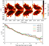 |
Fig. 1. 12-month average of the sunspot area (top) and centroid latitudes as a function of time starting from t0 (bottom). The dashed green lines represent the centroid latitude of the sunspot zone (Eq. (1)) and the vertical dashed lines the reference start times of the cycles (see text). |
We considered the average of the quantity f defined as
 (3)
(3)
n being the number of cycles that are averaged and nk(t) = n + i − k for t0k ≤ t < t0k + 1. The cycle-averaging was performed as follows: four copies of the data were made; then for each copy, i, the whole dataset was shifted back so that the cycle start times t0i and t01 coincide, whereafter the shifted copies were averaged together. We further symmetrized the data across the equator. Our procedure explicitly minimizes any north-south asymmetry, which will also contain information about the dynamo. The result for the 12-month average of the sunspot area is shown in Fig. 2. It consists of four averages of the solar cycles obtained by including a decreasing amount of cycles in the average.
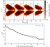 |
Fig. 2. Cycle average of the sunspot area (top) and centroid latitudes as a function of time starting from t0 (bottom). The dashed green lines represent the centroid latitude of the sunspot zone (Eq. (1)) and the vertical dashed lines the reference start times of the cycles (see the main text). |
3. The observed mean butterfly diagram
The WSO data we used are presented in Fig. 3 along with the reference start times of the individual cycles (see Sect. 2). By carrying out our cycle-averaging procedure, we obtained the time-latitude diagrams presented in Fig. 4. One can immediately see that the cycle-averaging produces butterfly wings that are much better defined. We have clear butterfly wings of one polarity, that of the leading sunspots, and poleward migrating fields of the opposite polarity, that of the trailing sunspots. The latter feature is also known as the ‘rush to the poles’ (Ananthakrishnan 1954; Altrock 1997). Even with only eight realizations, the trailing polarity field is essentially removed from the butterfly wings. The rush is also increasingly filled with fields of trailing polarity and is devoid of fields of leading polarity (see Fig. 3 of Mordvinov et al. 2022, for a more detailed look at the small-scale surges and features). We thus see a ‘separation of polarities’ happening. The butterfly wings are much more clearly delineated and seem narrower, with a width slightly under 30° rather than ≃35°. Lastly, the rapid increase in the sunspot number during the rising phase, and its slow decrease during the declining phase, is much more apparent.
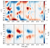 |
Fig. 3. Time-latitude diagrams of the surface radial field, Br (top), and surface toroidal field, Bϕ (bottom). The vertical dotted lines indicate the cycle start times as determined by the procedure outlined in Sect. 2. |
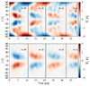 |
Fig. 4. Time-latitude diagrams of the mean surface radial field, |


It is clear, however, that four solar cycles is not nearly enough to carry out a proper ensemble average. It is nonetheless reasonable to assume that the addition of more cycles would only further the observed trend. Most of the small-scale features will be washed out and the mean observed butterfly diagram will look very similar to those calculated from mean-field dynamo models: smooth butterfly wings of the leading spot polarity, and a rush to the poles and polar fields of the trailing spot polarity.
We note the change of the scaling from Figs. 3 to 4: the largest fields inside the butterfly wings are reduced from 3 G to 2 G. Higher-resolution butterfly diagrams (e.g. Norton et al. 2023) have fields of the order of 10 G; in WSO data, part of the averaging has already been done by the instrument’s limited resolution. This is more evidence that one needs to be careful when comparing simulation results from mean-field models to observations.
4. Inferring the radial field generation rate
The radial field generation rate, or the radial source term, can be inferred both through the butterfly diagram and the time-latitude diagram of the surface toroidal field by using SFT and emergence (BL mechanism) models.
4.1. Surface flux transport model
The SFT model describes the passive advective and diffusive transport of the surface radial field via the following equation (Yeates et al. 2023):
![Mathematical equation: $$ \begin{aligned} \begin{aligned} \frac{\partial B_r}{\partial t}&=-\omega (\lambda )\frac{\partial B_r}{\partial \phi }-\frac{1}{R_\odot \cos \lambda }\frac{\partial }{\partial \lambda }\left(\cos \lambda { v}(\lambda )B_r\right)\\&\quad +\frac{\eta }{R_\odot ^2}\left[\frac{1}{\cos \lambda }\frac{\partial }{\partial \lambda }\left(\cos \lambda \frac{\partial B_r}{\partial \lambda }\right)+\frac{1}{\cos ^2\lambda }\frac{\partial ^2B_r}{\partial \phi ^2}\right]+S_r(\lambda ,\phi ,t), \end{aligned} \end{aligned} $$](/articles/aa/full_html/2024/11/aa50739-24/aa50739-24-eq6.gif) (4)
(4)
where Br, ω(λ), v(λ), η, and Sr(λ, ϕ, t) are respectively the surface radial field, angular velocity, meridional flow, diffusivity, and radial source term; λ is the latitude and ϕ the longitude. Since the magnetic butterfly diagram provides us with the longitudinally averaged surface radial field, Br(λ, t), the only unknown is the surface radial source term,
 (5)
(5)
We used a value of turbulent diffusivity of η = 350 km2/s, which is consistent with estimates from observations (e.g. Komm et al. 1995), the SFT model from Lemerle et al. (2015), and mixing length theory (e.g. Muñoz-Jaramillo et al. 2011). As for the surface meridional flow profile, we used the anti-symmetrized time-dependent profiles obtained from the helioseismic inversions of Gizon et al. (2020).
4.2. Emergence model
There is strong evidence (see e.g. Dasi-Espuig et al. 2010; Kitchatinov & Olemskoy 2011; Cameron & Schüssler 2015) that the BL mechanism is the main poloidal field generation mechanism of the solar dynamo. The first part of this mechanism is the emergence through the photosphere of tilted toroidal flux tubes. The corresponding generation of radial field from the emerging toroidal field is derived as follows.
We begin with the solenoidal condition  for an axisymmetric field, B,
 (6)
(6)
Next, we integrate in r from the surface to infinity and take the time derivative to obtain
 (7)
(7)
Joy’s law implies that as flux is emerging through the photosphere, Bθ = Bϕtanδ, where δ is the tilt angle of the resulting bipolar magnetic region (BMR). The rate at which the flux of Bϕ is carried through the surface per radian in θ is
 (8)
(8)
where ve is the radial velocity of the emerging field. Thus,
 (9)
(9)
This yields, for the surface radial field generation rate,
 (10)
(10)
or, with cosδ ∼ 1,
 (11)
(11)
We used the form of Joy’s law as given by Leighton (1969), sinδ = 0.5sinλ. As for the emergence velocity, we considered three different prescriptions. The first is the constant velocity of ve ≃ 200 m/s inferred by Centeno (2012); we also considered the cases where the emergence velocity, ve, is proportional to the toroidal field, Bϕ (Parker 1975) or to its square, Bϕ2 (Unno & Ribes 1976), mimicking magnetic buoyancy (Parker 1955a; Jensen 1955). We thus write the emergence velocity as
![Mathematical equation: $$ \begin{aligned} { v}_e=\left[\frac{|B_\phi |}{\max (B_\phi )}\right]^m { v}_0, \end{aligned} $$](/articles/aa/full_html/2024/11/aa50739-24/aa50739-24-eq15.gif) (12)
(12)
where v0 = 200 m/s and m ∈ {0, 1, 2}.
5. The observed mean radial field generation rate
The mean surface radial field generation rates,  , as inferred from the surface radial (Sect. 4.1) and toroidal fields (Sect. 4.2), are shown in Fig. 5. We clearly see one ‘mean BMR’ inside the activity belts. Remarkably, the two methods used to infer the radial field generation rate give results that are in good qualitative agreement, including for both the shape of the mean BMRs and their amplitudes. There are, however, three main noticeable discrepancies. Firstly, the SFT model gives us important radial field generation at the poles, of the opposite polarity to that of the polar fields. This could be explained by underestimated polar field strengths from the observations (Linker et al. 2017), possibly in combination with a weakened meridional flow amplitude at latitudes above 60° (Mahajan et al. 2021). Secondly, there are sorts of weak-amplitude ‘bridges’ at cycle minima between the poleward polarity of one cycle and the equatorward polarity of the next (showcasing the magnetic cycle and activity overlap between cycles). This overlap is only visible in the
  obtained through the surface toroidal field and Joy’s law. Thirdly, the source terms derived from the surface toroidal field and Joy’s law are slightly wider and are shifted slightly polewards compared to those obtained from the surface radial field.
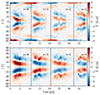 |
Fig. 5. Time-latitude diagrams of the mean surface radial source term, |

Lastly, we assumed that the emergence velocities of the toroidal field depend linearly and quadratically on the toroidal field strength. The result is presented in Fig. 6. We note that the cycle average was carried out after determining the surface radial source term. We see that increasing this dependence restricts the mean BMR to increasingly lower latitudes. Furthermore, in both the linear and quadratic cases, the aforementioned ‘bridges’ between sunspot cycles seen in the constant velocity case disappear. Since the bridges are absent in the  time-latitude diagram necessary to explain the evolution of the surface radial field, this suggests that either Joy’s law or the emergence velocity of low flux regions might differ from that of active regions.
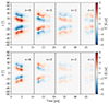 |
Fig. 6. Time-latitude diagrams of the mean surface radial source term, |

6. Conclusions
In this paper we have shown that one must be careful when comparing butterfly diagrams produced by simple mean-field models with observed ones. Because of imperfect scale separation, the use of the azimuthal average does not result in an observed butterfly diagram that can be understood in the mean-field sense. The observed butterfly diagram must for this purpose be cycle-averaged, a procedure made possible by the universality of the equatorward sunspot belt migration. From this standard law we can determine a reference time when all cycles are in phase with each other and can thus be meaningfully averaged. To ‘increase’ the small number of cycles for which magnetogram observations exist by a factor of two, we symmetrized both hemispheres together.
By making use of the average toroidal field time-latitude diagram and Joy’s law, we found that the α-effect-like BL source term is qualitatively consistent in shape and amplitude with the source term as inferred from the SFT model and the butterfly diagram. This consistency is further increased when we assume the toroidal field emergence velocity to be dependent on the toroidal field strength itself.
Downloaded from http://solarcyclescience.com/activeregions.html
Acknowledgments
The authors wish to thank the anonymous referee for comments that helped improve the overall quality of this paper. This work was carried out when SC was a member of the International Max Planck Research School for Solar System Science at the University of Göttingen. The authors acknowledge partial support from ERC Synergy grant WHOLE SUN 810218.
References
- Altrock, R. C. 1997, Sol. Phys., 170, 411 [NASA ADS] [CrossRef] [Google Scholar]
- Ananthakrishnan, R. 1954, Proc. Indian Acad. Sci. Math. Sci.-Sect. A, 40, 72 [CrossRef] [Google Scholar]
- Babcock, H. W. 1961, ApJ, 133, 572 [Google Scholar]
- Cameron, R., & Schüssler, M. 2015, Science, 347, 1333 [Google Scholar]
- Cameron, R. H., & Schüssler, M. 2023, Space Sci. Rev., 219, 60 [NASA ADS] [CrossRef] [Google Scholar]
- Cameron, R. H., Duvall, T. L., Schüssler, M., & Schunker, H. 2018, A&A, 609, A56 [NASA ADS] [CrossRef] [EDP Sciences] [Google Scholar]
- Centeno, R. 2012, ApJ, 759, 72 [NASA ADS] [CrossRef] [Google Scholar]
- Charbonneau, P. 2020, Liv. Rev. Sol. Phys., 17, 4 [Google Scholar]
- Dasi-Espuig, M., Solanki, S. K., Krivova, N. A., Cameron, R., & Peñuela, T. 2010, A&A, 518, A7 [NASA ADS] [CrossRef] [EDP Sciences] [Google Scholar]
- DeVore, C. R., Boris, J. P., Sheeley, N. R. J., 1984, Sol. Phys., 92, 1 [NASA ADS] [CrossRef] [Google Scholar]
- Gizon, L., Cameron, R. H., Pourabdian, M., et al. 2020, Science, 368, 1469 [Google Scholar]
- Hathaway, D. H. 2011, Sol. Phys., 273, 221 [NASA ADS] [CrossRef] [Google Scholar]
- Hathaway, D. H., Wilson, R. M., & Reichmann, E. J. 1994, Sol. Phys., 151, 177 [NASA ADS] [CrossRef] [Google Scholar]
- Hoyng, P. 2003, in Advances in nonlinear dynamos, eds. A. Ferriz-Mas, M. Núñez (London and New York: Taylor& Francis), 1 [Google Scholar]
- Jensen, E. 1955, Ann. Astrophys., 18, 127 [NASA ADS] [Google Scholar]
- Kitchatinov, L. L., & Olemskoy, S. V. 2011, Astron. Lett., 37, 656 [NASA ADS] [CrossRef] [Google Scholar]
- Komm, R. W., Howard, R. F., & Harvey, J. W. 1995, Sol. Phys., 158, 213 [NASA ADS] [Google Scholar]
- Leighton, R. B. 1964, ApJ, 140, 1547 [Google Scholar]
- Leighton, R. B. 1969, ApJ, 156, 1 [Google Scholar]
- Lemerle, A., Charbonneau, P., & Carignan-Dugas, A. 2015, ApJ, 810, 78 [NASA ADS] [CrossRef] [Google Scholar]
- Linker, J. A., Caplan, R. M., Downs, C., et al. 2017, ApJ, 848, 70 [NASA ADS] [CrossRef] [Google Scholar]
- Mahajan, S. S., Hathaway, D. H., Muñoz-Jaramillo, A., & Martens, P. C. 2021, ApJ, 917, 100 [NASA ADS] [CrossRef] [Google Scholar]
- Mordvinov, A. V., Karak, B. B., Banerjee, D., et al. 2022, MNRAS, 510, 1331 [Google Scholar]
- Muñoz-Jaramillo, A., Nandy, D., & Martens, P. C. H. 2011, ApJ, 727, L23 [NASA ADS] [CrossRef] [Google Scholar]
- Norton, A., Howe, R., Upton, L., & Usoskin, I. 2023, Space Sci. Rev., 219, 64 [CrossRef] [Google Scholar]
- Parker, E. N. 1955a, ApJ, 121, 491 [Google Scholar]
- Parker, E. N. 1955b, ApJ, 122, 293 [Google Scholar]
- Parker, E. N. 1975, ApJ, 198, 205 [NASA ADS] [CrossRef] [Google Scholar]
- Schou, J., Antia, H. M., Basu, S., et al. 1998, ApJ, 505, 390 [Google Scholar]
- Sheeley, N. R. J., DeVore, C. R., & Boris, J. P., 1985, Sol. Phys., 98, 219 [CrossRef] [Google Scholar]
- Steenbeck, M., Krause, F., & Rädler, K. H. 1966, Z. Naturforsch. Teil A, 21, 369 [NASA ADS] [CrossRef] [Google Scholar]
- Unno, W., & Ribes, E. 1976, ApJ, 208, 222 [NASA ADS] [CrossRef] [Google Scholar]
- Waldmeier, M. 1935, Astron. Mitt. Eidgenössischen Sternwarte Zürich, 14, 105 [Google Scholar]
- Waldmeier, M. 1939, Astron. Mitt. Eidgenössischen Sternwarte Zürich, 14, 470 [Google Scholar]
- Waldmeier, M. 1955, Ergebnisse und Probleme der Sonnenforschung (Leipzig: Akademische Verlagsgesellschaft Geest& Portig) [Google Scholar]
- Yeates, A. R., Cheung, M. C. M., Jiang, J., Petrovay, K., & Wang, Y.-M. 2023, Space Sci. Rev., 219, 31 [CrossRef] [Google Scholar]
All Figures
|
Fig. 1. 12-month average of the sunspot area (top) and centroid latitudes as a function of time starting from t0 (bottom). The dashed green lines represent the centroid latitude of the sunspot zone (Eq. (1)) and the vertical dashed lines the reference start times of the cycles (see text). |
| In the text | |
|
Fig. 2. Cycle average of the sunspot area (top) and centroid latitudes as a function of time starting from t0 (bottom). The dashed green lines represent the centroid latitude of the sunspot zone (Eq. (1)) and the vertical dashed lines the reference start times of the cycles (see the main text). |
| In the text | |
|
Fig. 3. Time-latitude diagrams of the surface radial field, Br (top), and surface toroidal field, Bϕ (bottom). The vertical dotted lines indicate the cycle start times as determined by the procedure outlined in Sect. 2. |
| In the text | |
|
Fig. 4. Time-latitude diagrams of the mean surface radial field, |
| In the text | |
|
Fig. 5. Time-latitude diagrams of the mean surface radial source term, |
| In the text | |
|
Fig. 6. Time-latitude diagrams of the mean surface radial source term, |
| In the text | |
Current usage metrics show cumulative count of Article Views (full-text article views including HTML views, PDF and ePub downloads, according to the available data) and Abstracts Views on Vision4Press platform.
Data correspond to usage on the plateform after 2015. The current usage metrics is available 48-96 hours after online publication and is updated daily on week days.
Initial download of the metrics may take a while.