| Issue |
A&A
Volume 680, December 2023
|
|
|---|---|---|
| Article Number | A42 | |
| Number of page(s) | 10 | |
| Section | The Sun and the Heliosphere | |
| DOI | https://doi.org/10.1051/0004-6361/202347022 | |
| Published online | 07 December 2023 | |
A Babcock-Leighton dynamo model of the Sun incorporating toroidal flux loss and the helioseismically inferred meridional flow
1
Max-Planck-Institut für Sonnensystemforschung, Justus-von-Liebig-Weg 3, 37077 Göttingen, Germany
e-mail: This email address is being protected from spambots. You need JavaScript enabled to view it.
2
Institut für Astrophysik und Geophysik, Georg-August-Universität Göttingen, 37077 Göttingen, Germany
Received:
26
May
2023
Accepted:
28
September
2023
Abstract
Context. Key elements of the Babcock-Leighton model for the solar dynamo are increasingly constrained by observations.
Aims. We investigate whether the Babcock-Leighton flux-transport dynamo model remains in agreement with observations if the meridional flow profile is taken from helioseismic inversions. Additionally, we investigate the effect of the loss of toroidal flux through the solar surface.
Methods. We employ the two-dimensional flux-transport Babcock-Leighton dynamo framework. We use the helioseismically inferred meridional flow profile, and include toroidal flux loss in a way that is consistent with the amount of poloidal flux generated by Joy’s law. Our model does not impose a preference for emergences at low latitudes; however, we do require that the model produces such a preference.
Results. We can find solutions that are in general agreement with observations, including the latitudinal migration of the butterfly wings and the 11 year period of the cycle. The most important free parameters in the model are the depth to which the radial turbulent pumping extends and the turbulent diffusivity in the lower half of the convection zone. We find that the pumping needs to extend to depths of about 0.80 R⊙ and that the bulk turbulent diffusivity needs to be around 10 km2 s−1 or less. We find that the emergences are restricted to low latitudes without the need to impose such a preference.
Conclusions. The flux-transport Babcock-Leighton model, incorporating the helioseismically inferred meridional flow and toroidal field loss term, is compatible with the properties of the observed butterfly diagram and with the observed toroidal loss rate. Reasonably tight constraints are placed on the remaining free parameters. The pumping needs to be just below the depth corresponding to the location where the meridional flow changes direction, and where numerical simulations suggest the convection zone becomes marginally subadiabatic. However, our linear model does not reproduce the observed ‘rush to the poles’ of the diffuse surface radial field resulting from the decay of sunspots; reproducing this might require the imposition of a preference for flux to emerge near the equator.
Key words: Sun: magnetic fields / Sun: activity / Sun: interior
© The Authors 2023
 Open Access article, published by EDP Sciences, under the terms of the Creative Commons Attribution License (https://creativecommons.org/licenses/by/4.0), which permits unrestricted use, distribution, and reproduction in any medium, provided the original work is properly cited.
This article is published in open access under the Subscribe to Open model.
Open access funding provided by Max Planck Society.
1. Introduction
The solar cycle is driven by a self-excited fluid dynamo that is induced by the interaction between the large-scale magnetic field and flows within the convection zone of the Sun (Ossendrijver 2003; Charbonneau 2014). In the first part of the dynamo loop, differential rotation winds up poloidal magnetic field generating toroidal field. This is the so-called Ω-effect. The Ω-effect is both well understood and constrained by observations.
In the second part of this loop, the toroidal field generates new poloidal magnetic field. This new poloidal field has the opposite polarity to the original poloidal field. Each 11 year sunspot (or Schwabe) cycle is half of the 22 year magnetic (or Hale) cycle required to revert to the original polarity. Non-axisymmetric flows and fields play a critical role during this phase of the cycle. However, the non-axisymmetric processes involved in the second phase are far from being either well understood or constrained.
A major success of helioseismology was the determination of the subsurface solar rotation profile, which challenged the dynamo-wave paradigm (Gough & Toomre 1991). This challenge lead to the flux-transport dynamo (FTD) model (Wang & Sheeley 1991), where the deep meridional circulation causes the emergence locations of sunspots to drift equatorwards during a solar cycle. Observational and theoretical studies (see e.g. Dasi-Espuig et al. 2010; Kitchatinov & Olemskoy 2011; Cameron & Schüssler 2015) provide strong support for the Babcock-Leighton (BL) mechanism (Babcock 1961; Leighton 1964, 1969) to be the dominant mechanism in the second part of the dynamo loop, as opposed to the turbulent α-effect (Parker 1955; Steenbeck et al. 1966). At the core of the BL mechanism is the role played by the surface field. Sunspots emerge in bipolar magnetic pairs, with an east–west orientation that is usually in accordance with Hale’s law. There is also a statistical tendency called Joy’s law for the leading spots to emerge closer to the equator and for the following spots to emerge closer to the poles. Sunspots decay within a few days to months, after which the field is dispersed by small-scale convective motions and transported poleward by the meridional flow. The flux cancellation of leading sunspot fields across the equator allows the net buildup of a polar field by trailing sunspot fields.
Transport processes are required at the surface in order to transport the radial field from the equator to the poles, and to transport the subsurface toroidal field equatorwards to account for the equatorial migration of the butterfly wings (Spörer’s law). The surface part of the required transport has been established by observations of the surface meridional flow and the success of the surface flux transport model. The helioseismically inferred subsurface meridional flow is a relatively new constraint for these models. The use of the helioseismically inferred meridional-flow profile removes a number of free parameters from BL-type models, which makes a comparison with observations a tighter test of the model and allows us to better constrain the remaining free parameters.
An additional recent constraint is that toroidal flux is lost through flux emergence, with a timescale estimated to be around 12 years by Cameron & Schüssler (2020, hereafter CS20). Here, we present an investigation of whether or not the BL FTD model – using the meridional flow inferred by Gizon et al. (2020, hereafter G20), and including the toroidal flux loss associated with flux emergence – is consistent with observations. To this end, we introduce a loss term in the evolution equation for the toroidal field that is consistent with the evolution of the poloidal flux associated with Joy’s law.
In the BL-type model considered in this paper, the turbulent convective motions are not explicitly simulated, instead their affect on the magnetic field is parameterized (e.g. Charbonneau 2014). Mean-field theory (Moffatt 1978; Krause & Rädler 1980) shows that including the effect of turbulence introduces a large number of parameters. In the BL model only a few are kept, the most important of which include the α-effect, an increased turbulent diffusion, and downward diamagnetic pumping. Of these, the BL α-effect is poorly understood but well constrained by observations, while turbulent pumping and turbulent diffusion are largely unconstrained.
In this paper, we show whether or not the FTD model – with the observed meridional flow and flux loss – is compatible with the BL model, and describe the constraints it places on the other processes of the model.
2. Model
2.1. Dynamo equations
In mean-field theory, the axisymmetric large-scale magnetic and velocity fields are decomposed into poloidal and toroidal components as
![Mathematical equation: $$ \begin{aligned}&\boldsymbol{B}=\nabla \times [A(r,\theta ,t)\boldsymbol{\hat{e}}_{\phi }]+B(r,\theta ,t)\boldsymbol{\hat{e}}_{\phi }, \end{aligned} $$](/articles/aa/full_html/2023/12/aa47022-23/aa47022-23-eq1.gif) (1)
(1)
 (2)
(2)
where A is the ϕ-component of the vector potential field and B is the toroidal component of the large-scale magnetic field, um is the meridional circulation, and Ω is the differential rotation. For an isotropic turbulent diffusivity that has only a r-dependence, the kinematic mean-field dynamo equations are
 (3)
(3)
![Mathematical equation: $$ \begin{aligned}&\frac{\partial B}{\partial t}=-\varpi \boldsymbol{u}_p\cdot \nabla \left(\frac{B}{\varpi }\right)+\eta \left(\nabla ^2-\frac{1}{\varpi ^2}\right)B+\frac{1}{\varpi }\frac{\partial (\varpi B)}{\partial r}\frac{\mathrm{d} \eta }{\mathrm{d} r}\nonumber \\ &\qquad \quad -B\nabla \cdot \boldsymbol{u}_p+\varpi [\nabla \times (A\boldsymbol{\hat{e}}_{\phi })]\cdot \nabla \Omega -L, \end{aligned} $$](/articles/aa/full_html/2023/12/aa47022-23/aa47022-23-eq4.gif) (4)
(4)
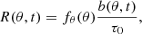
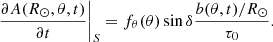
where ϖ = r sin θ, up = um + γ, η is the turbulent diffusivity, γ the turbulent pumping, S the BL source term, and L is the toroidal field loss term due to flux emergence. The source and loss terms are discussed in Sect. 2.4.
2.2. Differential rotation and meridional circulation
The large-scale flows need to be prescribed in kinematic models. For the differential rotation, we use the simple model provided by Belvedere et al. (2000) and shown in the left panel of Fig. 1:
 (5)
(5)
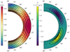 |
Fig. 1. Rotation profile of Belvedere et al. (2000) given by Eq. (5) (left) and the cycle-averaged and symmetrized stream function of the helioseismic meridional flow inversions of G20 (right). For the latter, positive values represent clockwise circulation and negative anticlockwise. The dash-dotted and dotted lines represent the approximate locations of the tachocline at 0.7 R⊙ and reversal of the meridional flow direction at 0.8 R⊙, respectively. |
where the coefficients cij can be found in this latter paper. This fit is an approximation of the helioseismologically inferred rotation rate of Schou et al. (1998).
As mentioned in Sect. 1, we use the meridional circulation inferred from observations. In this study, we use the inversions of G20. These authors furnish the meridional flow for cycles 23 and 24. In order to keep the parameter space study manageable, we take the average of the two cycles. In addition, as we are not presently interested in the asymmetry between both hemispheres, we also symmetrize the flow across the equator. The right panel of Fig. 1 shows the meridional circulation we use in all our models. We note that the flow switches from poleward to equatorward at a radius of about 0.785 R⊙, which we refer to as the meridional flow turnover depth rt; we refer to the region beneath it as the lower or deep convection zone, and the one above as the upper or shallow convection zone.
2.3. Turbulent parameterizations
We choose a turbulent diffusivity profile, which is written as a double step as in Muñoz-Jaramillo et al. (2011):
![Mathematical equation: $$ \begin{aligned}&\eta (r)=\eta _{\text{ RZ}}+ \frac{\eta _{\text{ CZ}}-\eta _{\text{ RZ}}}{2}\left[1+\text{ erf}\left(\frac{r-0.72R_\odot }{0.012R_\odot }\right)\right]\nonumber \\&\qquad \quad + \frac{\eta _{R_\odot }-\eta _{\text{ CZ}}-\eta _{\text{ RZ}}}{2}\left[1+\text{ erf}\left(\frac{r-0.95R_\odot }{0.01R_\odot }\right)\right], \end{aligned} $$](/articles/aa/full_html/2023/12/aa47022-23/aa47022-23-eq6.gif) (6)
(6)
where ηRZ = 0.1 km2 s−1, ηR⊙ = 350 km2 s−1, and ηCZ are respectively the radiative core, surface, and bulk values of the turbulent diffusivity. ηCZ is a free parameter and ηR⊙ has been chosen to be consistent with estimates from observations (e.g. Komm et al. 1995), the surface flux transport model of Lemerle et al. (2015), and MLT (e.g. Muñoz-Jaramillo et al. 2011). The values in the first error function have been chosen so that the drop in diffusivity occurs mostly before the helioseismically determined position of the tachocline (Charbonneau et al. 1999), roughly coinciding with the overshoot region (Christensen-Dalsgaard et al. 2011).
For the turbulent pumping, we adopt the profile given by Karak & Cameron (2016, hereafter KC16 – see also the discussion in their Sect. 2):
![Mathematical equation: $$ \begin{aligned} \boldsymbol{\gamma }=-\frac{\gamma _0}{2}\left[1+\text{ erf}\left(\frac{r-r_{\gamma }}{0.01R_\odot }\right)\right]\boldsymbol{\hat{e}}_r, \end{aligned} $$](/articles/aa/full_html/2023/12/aa47022-23/aa47022-23-eq7.gif) (7)
(7)
where here we take rγ = rt = 0.785 R⊙. This choice is discussed in Sect. 4.2.3.
2.4. Flux emergence
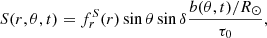
The emergence of bipolar magnetic regions both removes toroidal flux (see CS20) and creates poloidal flux (because of Joy’s law). These two processes are clearly linked, as are the respective loss and source terms in Eqs. (4) and (3).
We take the amount of flux emerging to be proportional to the toroidal flux density,
 (8)
(8)
where the integration is over the depth of the convection zone. This prescription corresponds to a dynamo where the toroidal field is not necessarily stored near the tachocline but can be distributed throughout the convection zone (KC16; Zhang & Jiang 2022). It is partly motivated by observations of dynamos in fully convective stars (Wright & Drake 2016), and partly by cyclic dynamo action in 3D magnetohydrodynamic (MHD) simulations of spherical shells without a tachocline (e.g. Brown et al. 2010; Nelson et al. 2013, 2014). The flux emergence rate R can be written in general as a function of latitude:
 (9)
(9)
where τ0 is a timescale and fθ(θ) is its latitudinal dependence, which we take to be
 (10)
(10)
corresponding to an emergence probability that is constant per unit length of the toroidal field lines.
In general, the timescale τ0 in Eq. (9) depends on the dynamics associated with flux emergence. If these dynamics are dominated by the large-scale field, then the buoyant rise time and τ0 depend inversely on the mean-field value of B2 (Kichatinov & Pipin 1993). However, if small-scale magnetic fields remain coherent over timescales longer than the correlation time, then the B filling factor – which can be far from 1 – becomes important. Some previous studies (e.g. Schmitt & Schüssler 1989; Moss et al. 1990a,b; Jennings & Weiss 1991) assume τ ∼ B−2 so that the loss term scales like B3. In this paper, we consider the linear case where τ0 is a constant; this corresponds to a case where the field is composed of filamentary structures with lifetimes longer than the correlation timescale of the turbulence and with local field strengths drawn from some distribution that is independent of flux. We stress that the aim in this paper is to consider a simple linear system. We defer the non-linear case to future work.
The orientation of the flux emergence is governed by Joy’s law, which states that the leading polarity flux emerges on average closer to the equator than the trailing polarity one. We take the form of Joy’s law used in Leighton (1969),  , where δ is the angle between the solar equator and the line joining the two polarities. The rate at which toroidal flux density is lost due to flux emergence is then
 (11)
(11)
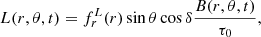
where the subscript L indicates the contribution from the loss term. The tilting of a toroidal flux tube as it emerges gives rise to a θ-component of the same polarity. The rate at which this θ-component of the flux density is lost is
 (12)
(12)
where the subscript S indicates the contribution from the source term S. This is what gives rise to the BL mechanism. From the definition of the poloidal field (Eq. (1)),
 (13)
(13)
We choose a depth Rb that is sufficiently below the base of the convection zone that the 11 year cyclic component of the field is negligible there. Then, multiplying both sides by r and integrating from the base of the convection zone to the surface, we obtain
![Mathematical equation: $$ \begin{aligned} \int _{R_b}^{R_\odot }B_\theta (r,\theta ,t)r\mathrm{d} r&=-\left[A(R_\odot ,\theta ,t)R_{\odot }-A(R_b,\theta ,t)R_b \right] \nonumber \\&=-A(R_\odot ,\theta ,t)R_{\odot }. \end{aligned} $$](/articles/aa/full_html/2023/12/aa47022-23/aa47022-23-eq15.gif) (14)
(14)
Therefore, in terms of the ϕ-component of the poloidal vector potential A, Eq. (12) becomes
 (15)
(15)
Next, we need to prescribe the radial structure of the source and loss terms. For the source term S, we follow KC16 and assume
 (16)
(16)
where
![Mathematical equation: $$ \begin{aligned} f_r^S(r)=\frac{1}{2}\left[1+\text{ erf}\left(\frac{r-r_S}{0.01R_\odot }\right)\right]. \end{aligned} $$](/articles/aa/full_html/2023/12/aa47022-23/aa47022-23-eq18.gif) (17)
(17)
Here, rS is the depth to which the source extends. For most of the calculations, we choose rS = 0.85 R⊙ (as in Muñoz-Jaramillo et al. 2010). There are indications that this disconnection should happen much deeper than the usually assumed shallow location of 0.95 R⊙ (Longcope & Choudhuri 2002). We nevertheless vary this parameter in order to study its impact on the solutions.
For the loss term L, we first distribute the toroidal flux density loss (Eq. (11)) over radius according to the amount of flux initially present, so that
 (18)
(18)
where
![Mathematical equation: $$ \begin{aligned} f_r^L(r)=\frac{1}{2}\left[1+\text{ erf}\left(\frac{r-0.70\,R_\odot }{0.01\,R_\odot }\right)\right]. \end{aligned} $$](/articles/aa/full_html/2023/12/aa47022-23/aa47022-23-eq20.gif) (19)
(19)
In order for the differential form of the source and loss terms to be valid, the emergence timescale τe must be considered infinitesimal with respect to the timescale over which the magnetic configuration of the large-scale field changes appreciably. It follows that a timescale separation must hold:
 (20)
(20)
In the case of the Sun, τe ∼ 1 day, and P = 11 years, and so the timescale separation is reasonable. This formulation implicitly ignores the effect of the meridional flow on the emergence process. Nevertheless, this formulation is sufficient to study the general features of the solar cycle.
2.5. Numerical procedure
Equations (3) and (4) are non-dimensionalized and are numerically solved in the meridional plane with 0 ≤ θ ≤ π and 0.65 R⊙ ≤ r ≤ R⊙. We use a spatial resolution of 241 × 301 evenly spaced in radius and colatitute grid points and a time step of 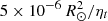 , where ηt = 10 km2 s−1. The inner boundary matches a perfect conductor, so that
 (21)
(21)
and the outer boundary condition is radial:
 (22)
(22)
The latter is necessary for FTD models to match models of surface flux transport (Cameron et al. 2012). A second-order centred finite difference discretization is used for the spatial variables and the solution is forwarded in time with the ADI scheme (Press et al. 1986). We use the code initially developed by D. Schmitt in Göttingen (as also used by Cameron et al. 2012).
The linearity of Eqs. (3) and (4) allows us to choose τ0 and γ0 such that the dynamo is approximately critical (σ ≤ 5 × 10⁻⁵ per year) with a cycle period of 12 years (within 0.1%), which is roughly the average period of cycles 23 and 24. This is how we reduce our parameter space to only one dimension (ηCZ). Our model being linear also means we can arbitrarily scale A and B. In order to facilitate comparisons with observations, we scale the fields so that the maximum of the surface radial field is 10 G, which is consistent with the observed polar field strengths at cycle minimum (e.g. Hathaway 2015).
3. Observational constraints
3.1. Toroidal flux loss timescale
The general expression for the toroidal flux decay timescale is
 (23)
(23)
where Φ is understood as the net subsurface toroidal flux in the northern hemisphere:
 (24)
(24)
and  is its decay. In order to calculate the latter, we first need to specify the toroidal flux loss mechanism. For the loss L due to flux emergence, we have
 (25)
(25)
and its corresponding timescale is denoted τL. Toroidal flux is also lost due to the explicit diffusion across the solar surface:
 (26)
(26)
with an associated diffusive loss timescale of τη. The observational constraint on the flux loss (or emergence loss) timescale is given by CS20, and corresponds to τL ≈ 12 years at solar maximum. As these timescales vary across a cycle, we calculate them at cycle maximum (defined in Sect. 3.2).
It is possible to estimate the range of values τ0 should take. To do so, we assume that the tilt angle δ associated with Joy’s law is small, so that cos δ ∼ 1, and that the toroidal flux density can be approximated by b(θ, t) = b0(t)sinmθ, where b0(t) is a time-dependent scalar, and m determines how closely the field is concentrated near the equator. With these approximations, we obtain
 (27)
(27)
where τ0 is the timescale for flux loss in the model, defined in Eq. (9), and the limits correspond to m = 0 and m = ∞. The model parameter τ0 should therefore be comparable to (not more than a factor of two smaller than) the observed toroidal flux loss timescale τL.
3.2. Polar cap and activity belt flux densities
An important observational constraint is that the maxima of azimuthally averaged polar flux densities should be around the same strength as maximum flux densities in the activity belt. As the evolution equations we are using are linear, we have nominally set the maximum of the polar field to 10 G. This implies that the azimuthaly averaged radial field in the butterfly wings in the model should also be around 10 G. We return to this constraint on the model when evaluating whether or not the model can produce solar-like cycles.
3.3. Cycle phase of polar maxima
An important constraint we take into account is the time of maximum polar flux. As it is observed to happen quite close to the activity minimum, its corresponding phase shift is about 90° with respect to cycle maximum. To measure this shift in the simulations, we need a definition of the time at which the cycle maxima and the maxima of polar fields occur.
We begin with the surface radial flux of the polar cap:
 (28)
(28)
and that of the activity belt:
 (29)
(29)
We then define cycle maximum times, Ta, as the times when the activity belt flux Φa is maximum. The time of the maximum polar flux Tp is similarly defined. Ta and Tp are both defined by the signed fluxes, and hence each has one maximum per magnetic cycle (of about 24 years).
For each cycle, i, we then calculate the phase shift between the polar maximum times and the activity maximum times Δϕ using
![Mathematical equation: $$ \begin{aligned} \Delta \phi =\pi [T_p(i+1)-T_a(i)] /P-\pi , \end{aligned} $$](/articles/aa/full_html/2023/12/aa47022-23/aa47022-23-eq33.gif) (30)
(30)
where P is the (activity) cycle period.
4. Results
We first present our reference model including the BL loss term in Sect. 4.1, and then examine parameter sensitivity (Sects. 4.2–4.5), and finally gauge the importance of the dynamo wave (Sect. 4.6).
4.1. Reference model
Our reference model has a bulk diffusivity of ηCZ = 10 km2 s−1, which places the simulation in the advection-dominated regime (an explanation of why such a low diffusivity is required in our setup is given in Sect. 4.2.2). Values of τ0 = 12.5 years and γ0 = 43.8 m s−1 were required to achieve a critical 12 year (activity) cycle period dynamo. The reference model is presented in Fig. 2. It can be seen that we are able to produce a reasonably solar-like butterfly diagram when using the helioseismically inferred meridional flow of G20.
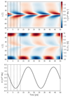 |
Fig. 2. Time–latitude diagrams of the toroidal flux density b (top), surface radial field Br(R⊙) (middle), and the net toroidal flux in the northern hemisphere Φ (bottom) for our reference model. The vertical dotted lines indicate the times where the snapshots of Fig. 3 were taken. |
This model has an emergence loss timescale of τL = 17.2 years, which is somewhat longer than the 12 years inferred by CS20. The diffusive loss timescale, on the other hand, is τη = 96.8 years. The estimate of CS20 is based on all toroidal flux escaping through the photosphere. The combined rate at which flux is lost through the photosphere in the model can be estimated to be 1/(1/τL + 1/τη) = 14.6 years, which is close to the inferred 12 year timescale. The value of Δϕ from the model is noticeably larger than the observed value at Δϕ = 134°. The maximum value of the surface radial field in the butterfly wings is around 5 G, which is about half of the maximum polar field strength (the observed average polar field is similar to the average in the butterfly wings; see e.g. the butterfly diagrams in Hathaway 2015). Considering that the polar field strength is somewhat uncertain, our results are not inconsistent with observations. Our simulations do not have the problem of very large polar fields typical of FTD models (Charbonneau 2020). The net toroidal flux Φ (lower panel of Fig. 3) shows that it reaches a maximum value of about 5 × 10²³ Mx close to cycle maximum, which is in rather good agreement with the estimates of Cameron & Schüssler (2015) for cycles 22 and 23.
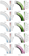 |
Fig. 3. Meridional cuts of the northern hemisphere toroidal field (left column) and poloidal field (as r sin θA, right column) of the reference model for specific times indicated by the vertical dotted lines in Fig. 2. The dotted lines are located at radii of 0.95, 0.85, and 0.80 R⊙, the approximate locations of the bottom of the near-surface shear layer, rS, and rγ, respectively. |
An important result of our model is that it achieves confinement of emergences to the low observed latitudes without the need for an emergence probability decreasing faster than sin θ with latitude. This can be seen in the upper panel of Fig. 2, where we see that the toroidal flux density is mainly strong near the equator. The left panel of Fig. 3 shows the toroidal field is mainly stored deep in the convection zone. This confinement of the toroidal field deep in the convection zone is a consequence of the imposed radial pumping. The confinement to near the equator is then due to the meridional flow, which advects the material from high latitudes towards the equator. The combination of radial pumping and equatorward meridional flow in the lower half of the convection zone leads to a stagnation point near the equator in the lower half of the convection zone, where the field builds up until it is removed through emergence (also see Cameron & Schüssler 2017; Jiang et al. 2013). Our simulated butterfly diagram differs from the observed one in that it lacks a distinct ‘rush to the poles’ of the trailing diffuse field of the decayed sunspots.
4.2. Parameter dependence
Our model has five free parameters: the source and loss term timescale τ0 and the depth where sunspots are anchored rS, the turbulent pumping amplitude γ0 and the depth it reaches down to rγ, and the turbulent diffusivity in the bulk of the convection zone ηCZ. In this section, we first provide a qualitative description of the end result of different choices of the parameters.
Importantly, the results and constraints we find are for a scenario in which we assume that fθ(θ) = sin θ, that is, that there is no imposed preference for emergences to occur at low latitudes. We also performed simulations with fθ(θ) = sin12θ (as in KC16), and as expected were able to find critical dynamo solutions that match the observations for a much wider range of parameters.
4.2.1. Influence of the source depth
Here, we present our investigation of how the choice of rS affects the solutions. We used the same value of ηCZ as in the reference case, and varied rS. The values of τ0 and γ0 were then chosen so that the growth rate is zero and the cycle period is 12 years. We find that the solutions with flux loss are not very dependent on rS for rS extending from just above 0.78 to the surface. This is because the solutions with flux loss require strong pumping, which rapidly stretches the poloidal field so that it extends radially to the depth at which the pumping stops. This makes the model insensitive to the depth of the poloidal source term (at least in the region of parameter space near the reference case).
4.2.2. The bulk diffusivity
We only find critical 12 year periodic solutions when the bulk diffusivity is of the order of 10 km2 s−1. This is a consequence of the strong radial shear of the equatorward component of the helioseismically inferred meridional flow uθ in the lower third of the convection zone. The strong radial shear leads to toroidal flux at different depths being advected in latitude at very different rates. This implies that flux originally concentrated at one latitude over a range of depths will be quickly spread out in latitude.
To understand the role of the radial shear of the latitudinal flow, we can imagine toroidal field initially at one latitude but spread out in radius from r = 0.766 R⊙ to 0.785 R⊙. These depths were chosen so that the meridional flow varies from almost 1 m s−1 equatorwards to almost 0 m s−1. Over 5 years, this will spread the flux over a latitudinal band of 157 Mm. This spreading out would be similar to a diffusivity of (157)2/5 Mm2 year−1 = 156 km2 s−1. In the context of BL FTD models, this is a large value. As a comparison, the 1D model of Cameron & Schüssler (2017), which also assumes fθ(θ) = sin θ, requires that the latitudinal diffusivity in the bulk of the convection zone be lower than about 100 km2 s−1. However, this effective diffusivity is in agreement with the estimate of Cameron & Schüssler (2016) of 150 − 450 km2 s−1 based on the properties of the declining phase of the solar cycle.
In summary, unless the toroidal field is confined to a narrow range of depths, the latitudinal shear in the meridional velocity quickly spreads the toroidal field out in latitude. Consequently, if there is no imposed preference for emerging near the equator then the butterfly diagram ceases to be solar-like. The requirement for confinement in latitude is what imposes the constraint that ηCZ ≈ 10 km2 s−1. We consider this fixed for the rest of this paper. We also mention that if the radial shear in the differential rotation were weaker, then this constraint would be much weaker.
4.2.3. Turbulent magnetic pumping
With our chosen fθ(θ) = sin θ (Eq. (10)), we only find growing dynamo solutions for values of rγ that are not far away from 0.785 R⊙. This depth is where the helioseismically inferred meridional flow profile changes direction from poleward to equatorward, and roughly where numerical simulations suggest the convection zone might be weakly subadiabatic (Hotta 2017). A slightly broader range of pumping depths can be achieved when the loss term is not included, but shallower depths make the butterfly wings broader.
Our conclusion from this is that the pumping depth is fairly tightly constrained if the appearance of spots to low latitudes is only caused by the equatorward meridional flow leading to a build up at low latitudes. The depth of the pumping is poorly constrained if the preference for low-latitude emergence is imposed.
Observations do not provide estimates of the amplitude of turbulent pumping at depth, and so it is interesting to compare our results with those from global MHD simulations. Shimada et al. (2022) find that the outer half of the convection zone has a turbulent diffusivity of ∼10 km2 s−1, similar to the values we needed in our model without an imposed preference for emergence at low latitudes. These authors also find that γr peaks at ∼10 m s−1, while Simard et al. (2016) and Warnecke et al. (2018) find amplitudes of the order of 1 − 2 m s−1 or half the root-mean-square velocity. The latter is of the order of 40 m s−1 according to mixing-length (Vitense 1953; Böhm-Vitense 1958) estimates. It therefore appears the pumping velocities required in the reference case are too large by a factor of 2 to 3. We defer a discussion of this to Sects. 4.4 and 4.5.
4.3. Role of the toroidal flux loss term L
In order to gauge the importance of the emergence loss term, in this subsection we switch off the term by setting L = 0 in Eq. (4). We first use the same parameters as in the reference case. The resulting cycle period is shorter at 11.3 years. However, the solution is rapidly growing, with a growth rate of about 66% per cycle. This growth is not unexpected, as emergences are no longer able to remove the subsurface toroidal flux and it must now be removed either through its ‘unwinding’ by the new cycle flux, or by diffusive cancellation across the equator. Because emergences no longer deplete the subsurface toroidal flux, more poloidal field is generated so that the polar fields are reversed much faster, explaining the shorter period.
We also investigated the 12 year period critical solutions when L = 0. Doing so required τ0 = 9.3 years (as opposed to the reference case, where τ0 = 12.5 years), and a turbulent pumping γ0 = 6.41 m s−1. The time–latitude diagrams and meridional cuts for this case are shown in Figs. 4 and 5. The surface diffusion loss timescale is reduced to τη = 25.6 years, which is only a factor of two larger than the observed value of the toroidal flux loss timescale. This is due to the lowered pumping amplitude, which makes the diffusion of the toroidal field through the surface less difficult than in the case with strong pumping. Even with such low pumping, the poloidal field near the surface is still almost radial (Fig. 5).
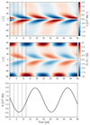 |
Fig. 4. Time–latitude diagrams of the toroidal flux density b (top), surface radial field Br(R⊙) (middle), and the net toroidal flux in the northern hemisphere Φ (bottom) for the case without the flux loss associated with flux emergence (and with a period of 12 years and zero growth rate). The vertical dotted lines indicate the times where the snapshots of Fig. 5 were taken. |
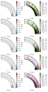 |
Fig. 5. Meridional cuts of the northern hemisphere toroidal field (left column) and poloidal field (as r sin θA, right column) in the case without the flux loss associated with flux emergence (and with a period of 12 years and zero growth rate) for specific times indicated by the vertical dotted lines in Fig. 4. The dotted lines are located at radii of 0.95, 0.85, and 0.80 R⊙, the approximate locations of the bottom of the near-surface shear layer, rS, and rγ, respectively. |
Looking at the butterfly diagram, the most apparent difference is the large decrease in the polar field strengths compared to the fields in the butterfly wings. The maximum value of the latter goes up from about 5 to 7.5 G, which is relatively close to the observed value of around 10 G. In this case, we find that the phase between the polar field maxima and active region maxima Δϕ is 101°, similar to that which is observed.
We note that the pumping amplitude of γ0 = 6.41 m s−1 in this model is in much better agreement with estimates from global MHD simulations (cf. Sect. 4.2.3). This is because models without the loss term achieve shorter periods much more easily. In principle, very large pumping velocities are therefore not necessary in order to obtain a functioning dynamo for this class of models.
4.4. Sensitivity to the meridional flow and differential rotation
Here we investigate how sensitive the simulations are to the meridional flow and differential rotation. We do this by considering the inferred meridional flow for cycles 23 and 24 separately, and a differential rotation profile that differs significantly from that of the reference model at high latitudes. As is also the case for the reference solution, we do not impose a preference for emergences at low latitudes (if we impose a preference for emergences at low latitudes, then the parameter space where the model has similar properties to the observations becomes much larger). As all solutions mentioned in this section have qualitatively the same butterfly diagrams as the reference case, they are not shown.
First, we consider the symmetrized (across the equator) meridional flow profiles of cycles 23 and 24 individually. Using the meridional flow from cycle 23, a 12 year periodic critical dynamo requires γ0 = 16.3 m s−1. This is a substantial reduction from the reference case. Increasing the period to 13.3 years and keeping the criticality requirement led to pumping speeds of γ0 = 10 m s−1. Using the meridional flow from cycle 24, we were unable to find critical solutions with periods of shorter than 12 years. A critical solution with γ0 = 10 m s−1 required a period of 16.6 years.
Clearly the model, where emergence is not restricted to low latitudes is very sensitive to the meridional flow. This is because emergences at high latitudes are inefficient at getting flux across the equator, which is what eventually reverses the polar fields. The observational constraint that the cycle period is similar to the timescale over which toroidal field is lost through the surface due to flux emergence implies that the cycle period involves a balance between the flux transport to low latitudes and the loss through emergence.
In this context, both mean-field theory (e.g. Kichatinov 1991; Kitchatinov & Nepomnyashchikh 2016) and global numerical models (e.g. Shimada et al. 2022, and references therein) indicate equatorial latitudinal turbulent pumping could also be substantial. From the BL-FTD modelling, this would correspond to an increase in the meridional return flow, and would lead to a reduction in the strength of the required radial pumping.
Second, we consider the sensitivity to differential rotation. Again we consider critical 12 year periodic solutions, using the average meridional flow profile used in the reference case. We now use the differential rotation profile of Larson & Schou (2018), which differs from that of the reference at high latitudes (rather than the analytic fit of Belvedere et al. (2000) often used in dynamo studies and used in the reference case). The required parameter values are τ0 = 11.8 yr and γ0 = 28.5 m s−1. τ0 is again of the order of the cycle period and the 12 year estimate for the toroidal flux loss timescale of Cameron & Schüssler (2020). However, the pumping velocity is much more reasonable.
4.5. Sensitivity to the assumptions of zero growth rate and a 12 year period
Above, we concentrate on the kinematic regime with zero growth rates. The Sun is certainly in a statistically saturated state. The kinematic case with zero growth rate is relevant if the system is weakly non-linear. Whether or not this is the case for the Sun is an open question (for arguments in favour of this, see van Saders et al. 2016; Metcalfe et al. 2016; Kitchatinov & Nepomnyashchikh 2017). In the strongly non-linear case, the period will be substantially affected by the choice of the non-linearity and the growth rate in the linear regime is no longer a constraint. The observations are therefore less constraining in the strongly non-linear case. For this reason, we focus on the weakly non-linear case and looked for zero-growth-rate solutions to the linear problem. The addition of a weak non-linearity will slightly modify both the growth rate (in the saturated state it will be zero) and period. In this section, we therefore consider the sensitivity of the growth rate and periods to τ0 and γ0.
Figure 6 shows the cycle period and the growth of the toroidal flux per cycle as a function of the timescale parameter τ0. As in KC16, we observe that increasing the source term amplitude  causes the growth rate to increase until the cycle period becomes too short for the meridional flow to transport the field (see Sect. 4.1 of KC16). Eventually, the dynamo shuts down completely. Growing solutions can nonetheless be reached by further increasing the source term amplitude
  . However, the resulting cycle periods are very short (≲3 years) and the dynamo is now driven by a dynamo wave propagating equatorwards in the high-latitude tachocline.
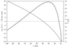 |
Fig. 6. Percentage per-cycle growth of the toroidal flux (solid line, left axis) and cycle period (dashed line, right axis) as a function of the timescale parameter τ0. |
The effect of the pumping amplitude on the growth rate and cycle period is shown in Fig. 7. The growth rate is very sensitive to the pumping amplitude at lower values, where the operating threshold is not yet met, as flux emergence then quickly removes the toroidal flux at high latitudes. However, the effect of pumping saturates as its amplitude increases. At some point the time required for the poloidal field to reach the lower convection zone is almost negligible. We note that here we concentrate on solutions near the bifurcation point where dynamo action switches on. This very likely makes the model more sensitive to the different parameters than would be the case if we were considering a non-linear, saturated dynamo.
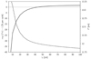 |
Fig. 7. Percentage per-cycle growth of the toroidal flux (solid line, left axis) and cycle period (dashed line, right axis) as a function of pumping amplitude γ0. |
4.6. Role of the dynamo wave
To investigate what role the subsurface meridional return flow is playing, we apply the same procedure as KC16 to our reference model; namely we switch off the equatorward component of the meridional flow (see Sect. 3.2 of KC16 for a discussion). Figure 8 shows the resulting magnetic field butterfly diagram. For the reference parameters, this mode is decaying (and so is not a dynamo) with fields almost entirely located above 45°. As there is no equatorward component of the meridional flow, the equatorward migration of the field is due to the negative radial rotation shear in the high-latitude tachocline, and the direction of propagation is in accordance with the Parker-Yoshimura sign rule. Unsurprisingly, we therefore conclude that the subsurface meridional flow is essential in this model.
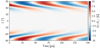 |
Fig. 8. Butterfly diagram of our reference model where the equatorward component of the meridional flow is shut off. |
5. Conclusion
Using the helioseismically inferred meridional flow of G20, we show that the BL FTD model remains generally consistent with observations. We also show that the long-standing problem of the latitudinal distribution of sunspots can be solved if turbulent pumping reaches depths of just under 0.80 R⊙ but not significantly deeper, where the direction of the meridional flow switches from poleward to equatorward. High turbulent pumping velocities are necessary to contain the toroidal flux in this location, in agreement with the results of G20 (see also Parker 1987). There, the meridional flow, in conjunction with the Ω-effect through the latitudinal shear present in the bulk of the convection zone (which is maximal at mid-latitudes), causes an accumulation of toroidal flux at equatorial latitudes. Turbulent pumping effectively short-circuits the meridional circulation, preventing significant generation of toroidal field at high latitudes. No additional restriction of emergences to low latitudes is required.
Our model, which uses the helioseismically inferred meridional flow and includes the observed toroidal flux loss associated with flux emergence in a way that is consistent with the BL source term, is able to reproduce the observed properties of the solar cycle, including the latitudinal migration of the sunspot wings and the approximately 11 year period. Our reference model predicts a toroidal flux loss timescale of 14.8 years at cycle maximum, as opposed to the estimate of 12 years of CS20.
Acknowledgments
The authors wish to thank the anonymous referee for comments that helped improve the overall quality of this paper. SC is a member of the International Max Planck Research School for Solar System Science at the University of Göttingen. The authors acknowledge partial support from ERC Synergy grant WHOLE SUN 810218.
References
- Babcock, H. W. 1961, ApJ, 133, 572 [Google Scholar]
- Belvedere, G., Kuzanyan, K. M., & Sokoloff, D. 2000, MNRAS, 315, 778 [NASA ADS] [CrossRef] [Google Scholar]
- Böhm-Vitense, E. 1958, ZAp, 46, 108 [NASA ADS] [Google Scholar]
- Brown, B. P., Browning, M. K., Brun, A. S., Miesch, M. S., & Toomre, J. 2010, ApJ, 711, 424 [Google Scholar]
- Cameron, R., & Schüssler, M. 2015, Science, 347, 1333 [Google Scholar]
- Cameron, R. H., & Schüssler, M. 2016, A&A, 591, A46 [NASA ADS] [CrossRef] [EDP Sciences] [Google Scholar]
- Cameron, R. H., & Schüssler, M. 2017, A&A, 599, A52 [NASA ADS] [CrossRef] [EDP Sciences] [Google Scholar]
- Cameron, R. H., & Schüssler, M. 2020, A&A, 636, A7 [NASA ADS] [CrossRef] [EDP Sciences] [Google Scholar]
- Cameron, R. H., Schmitt, D., Jiang, J., & Işık, E. 2012, A&A, 542, A127 [NASA ADS] [CrossRef] [EDP Sciences] [Google Scholar]
- Charbonneau, P. 2014, ARA&A, 52, 251 [NASA ADS] [CrossRef] [Google Scholar]
- Charbonneau, P. 2020, Liv. Rev. Sol. Phys., 17, 4 [Google Scholar]
- Charbonneau, P., Christensen-Dalsgaard, J., Henning, R., et al. 1999, ApJ, 527, 445 [NASA ADS] [CrossRef] [Google Scholar]
- Christensen-Dalsgaard, J., Monteiro, M. J. P. F. G., Rempel, M., & Thompson, M. J. 2011, MNRAS, 414, 1158 [CrossRef] [Google Scholar]
- Dasi-Espuig, M., Solanki, S. K., Krivova, N. A., Cameron, R., & Peñuela, T. 2010, A&A, 518, A7 [NASA ADS] [CrossRef] [EDP Sciences] [Google Scholar]
- Gizon, L., Cameron, R. H., Pourabdian, M., et al. 2020, Science, 368, 1469 [Google Scholar]
- Gough, D., & Toomre, J. 1991, ARA&A, 29, 627 [NASA ADS] [CrossRef] [Google Scholar]
- Hathaway, D. H. 2015, Liv. Rev. Sol. Phys., 12, 4 [Google Scholar]
- Hotta, H. 2017, ApJ, 843, 52 [Google Scholar]
- Jennings, R. L., & Weiss, N. O. 1991, MNRAS, 252, 249 [Google Scholar]
- Jiang, J., Cameron, R. H., Schmitt, D., & Işık, E. 2013, A&A, 553, A128 [NASA ADS] [CrossRef] [EDP Sciences] [Google Scholar]
- Karak, B. B., & Cameron, R. 2016, ApJ, 832, 94 [NASA ADS] [CrossRef] [Google Scholar]
- Kichatinov, L. L. 1991, A&A, 243, 483 [NASA ADS] [Google Scholar]
- Kitchatinov, L. L., & Nepomnyashchikh, A. A. 2016, Adv. Space Res., 58, 1554 [NASA ADS] [CrossRef] [Google Scholar]
- Kitchatinov, L., & Nepomnyashchikh, A. 2017, MNRAS, 470, 3124 [NASA ADS] [CrossRef] [Google Scholar]
- Kitchatinov, L. L., & Olemskoy, S. V. 2011, Astron. Lett., 37, 656 [NASA ADS] [CrossRef] [Google Scholar]
- Kichatinov, L. L., & Pipin, V. V. 1993, A&A, 274, 647 [NASA ADS] [Google Scholar]
- Komm, R. W., Howard, R. F., & Harvey, J. W. 1995, Sol. Phys., 158, 213 [NASA ADS] [Google Scholar]
- Krause, F., & Rädler, K. H. 1980, Mean-field Magnetohydrodynamics and Dynamo theory (Oxford: Pergamon Press) [Google Scholar]
- Larson, T. P., & Schou, J. 2018, Sol. Phys., 293, 29 [Google Scholar]
- Leighton, R. B. 1964, ApJ, 140, 1547 [Google Scholar]
- Leighton, R. B. 1969, ApJ, 156, 1 [Google Scholar]
- Lemerle, A., Charbonneau, P., & Carignan-Dugas, A. 2015, ApJ, 810, 78 [NASA ADS] [CrossRef] [Google Scholar]
- Longcope, D., & Choudhuri, A. R. 2002, Sol. Phys., 205, 63 [NASA ADS] [CrossRef] [Google Scholar]
- Metcalfe, T. S., Egeland, R., & van Saders, J. 2016, ApJ, 826, L2 [Google Scholar]
- Moffatt, H. K. 1978, Magnetic Field Generation in Electrically Conducting Fluids (Cambridge: University Press) [Google Scholar]
- Moss, D., Tuominen, I., & Brandenburg, A. 1990a, A&A, 240, 142 [NASA ADS] [Google Scholar]
- Moss, D., Tuominen, I., & Brandenburg, A. 1990b, A&A, 228, 284 [NASA ADS] [Google Scholar]
- Muñoz-Jaramillo, A., Nandy, D., Martens, P. C. H., & Yeates, A. R. 2010, ApJ, 720, L20 [CrossRef] [Google Scholar]
- Muñoz-Jaramillo, A., Nandy, D., & Martens, P. C. H. 2011, ApJ, 727, L23 [NASA ADS] [CrossRef] [Google Scholar]
- Nelson, N. J., Brown, B. P., Brun, A. S., Miesch, M. S., & Toomre, J. 2013, ApJ, 762, 73 [Google Scholar]
- Nelson, N. J., Brown, B. P., Brun, A. S., Miesch, M. S., & Toomre, J. 2014, Sol. Phys., 289, 441 [NASA ADS] [CrossRef] [Google Scholar]
- Ossendrijver, M. 2003, A&ARv, 11, 287 [Google Scholar]
- Parker, E. N. 1955, ApJ, 122, 293 [Google Scholar]
- Parker, E. N. 1987, Sol. Phys., 110, 11 [NASA ADS] [CrossRef] [Google Scholar]
- Press, W. H., Flannery, B. P., & Teukolsky, S. A. 1986, Numerical Recipes. The Art of Scientific Computing (Cambridge: University Press) [Google Scholar]
- Schmitt, D., & Schüssler, M. 1989, A&A, 223, 343 [NASA ADS] [Google Scholar]
- Schou, J., Antia, H. M., Basu, S., et al. 1998, ApJ, 505, 390 [Google Scholar]
- Shimada, R., Hotta, H., & Yokoyama, T. 2022, ApJ, 935, 55 [NASA ADS] [CrossRef] [Google Scholar]
- Simard, C., Charbonneau, P., & Dubé, C. 2016, Adv. Space Res., 58, 1522 [NASA ADS] [CrossRef] [Google Scholar]
- Steenbeck, M., Krause, F., & Rädler, K. H. 1966, Zeitschrift Naturforschung Teil A, 21, 369 [NASA ADS] [CrossRef] [Google Scholar]
- van Saders, J. L., Ceillier, T., Metcalfe, T. S., et al. 2016, Nature, 529, 181 [Google Scholar]
- Vitense, E. 1953, ZAp, 32, 135 [Google Scholar]
- Wang, Y. M., Sheeley, N. R. J., & Nash, A. G., 1991, ApJ, 383, 431 [NASA ADS] [CrossRef] [Google Scholar]
- Warnecke, J., Rheinhardt, M., Tuomisto, S., et al. 2018, A&A, 609, A51 [NASA ADS] [CrossRef] [EDP Sciences] [Google Scholar]
- Wright, N. J., & Drake, J. J. 2016, Nature, 535, 526 [Google Scholar]
- Zhang, Z., & Jiang, J. 2022, ApJ, 930, 30 [NASA ADS] [CrossRef] [Google Scholar]
All Figures
|
Fig. 1. Rotation profile of Belvedere et al. (2000) given by Eq. (5) (left) and the cycle-averaged and symmetrized stream function of the helioseismic meridional flow inversions of G20 (right). For the latter, positive values represent clockwise circulation and negative anticlockwise. The dash-dotted and dotted lines represent the approximate locations of the tachocline at 0.7 R⊙ and reversal of the meridional flow direction at 0.8 R⊙, respectively. |
| In the text | |
|
Fig. 2. Time–latitude diagrams of the toroidal flux density b (top), surface radial field Br(R⊙) (middle), and the net toroidal flux in the northern hemisphere Φ (bottom) for our reference model. The vertical dotted lines indicate the times where the snapshots of Fig. 3 were taken. |
| In the text | |
|
Fig. 3. Meridional cuts of the northern hemisphere toroidal field (left column) and poloidal field (as r sin θA, right column) of the reference model for specific times indicated by the vertical dotted lines in Fig. 2. The dotted lines are located at radii of 0.95, 0.85, and 0.80 R⊙, the approximate locations of the bottom of the near-surface shear layer, rS, and rγ, respectively. |
| In the text | |
|
Fig. 4. Time–latitude diagrams of the toroidal flux density b (top), surface radial field Br(R⊙) (middle), and the net toroidal flux in the northern hemisphere Φ (bottom) for the case without the flux loss associated with flux emergence (and with a period of 12 years and zero growth rate). The vertical dotted lines indicate the times where the snapshots of Fig. 5 were taken. |
| In the text | |
|
Fig. 5. Meridional cuts of the northern hemisphere toroidal field (left column) and poloidal field (as r sin θA, right column) in the case without the flux loss associated with flux emergence (and with a period of 12 years and zero growth rate) for specific times indicated by the vertical dotted lines in Fig. 4. The dotted lines are located at radii of 0.95, 0.85, and 0.80 R⊙, the approximate locations of the bottom of the near-surface shear layer, rS, and rγ, respectively. |
| In the text | |
|
Fig. 6. Percentage per-cycle growth of the toroidal flux (solid line, left axis) and cycle period (dashed line, right axis) as a function of the timescale parameter τ0. |
| In the text | |
|
Fig. 7. Percentage per-cycle growth of the toroidal flux (solid line, left axis) and cycle period (dashed line, right axis) as a function of pumping amplitude γ0. |
| In the text | |
|
Fig. 8. Butterfly diagram of our reference model where the equatorward component of the meridional flow is shut off. |
| In the text | |
Current usage metrics show cumulative count of Article Views (full-text article views including HTML views, PDF and ePub downloads, according to the available data) and Abstracts Views on Vision4Press platform.
Data correspond to usage on the plateform after 2015. The current usage metrics is available 48-96 hours after online publication and is updated daily on week days.
Initial download of the metrics may take a while.