| Issue |
A&A
Volume 693, January 2025
|
|
|---|---|---|
| Article Number | A89 | |
| Number of page(s) | 8 | |
| Section | The Sun and the Heliosphere | |
| DOI | https://doi.org/10.1051/0004-6361/202450170 | |
| Published online | 06 January 2025 | |
Investigating numerical stability by scaling heat conduction in a 1D hydrodynamic model of the solar atmosphere
1
Institute of Physics, University of Graz, Universitätspl. 5, 8010 Graz, Austria
2
Space Research Institute, Austrian Academy of Sciences, Schmiedlstr. 6, 8042 Graz, Austria
⋆ Corresponding author; This email address is being protected from spambots. You need JavaScript enabled to view it.
Received:
28
March
2024
Accepted:
8
December
2024
Abstract
Context. Numerical models of the solar atmosphere are widely used in solar research and provide insights into unsolved problems such as the heating of coronal loops. A prerequisite for such simulations is an initial condition for the plasma temperature and density. Many explicit numerical schemes employ high-order derivatives that require some diffusion, for example isotropic diffusion, for each independent variable to maintain numerical stability. Otherwise, significant numerical inaccuracies and subsequent wiggles will occur and grow at steep temperature gradients in the solar transition region.
Aims. We tested how to adapt the isotropic heat conduction to the grid resolution so that the model is capable of resolving varying temperature gradients. Our ultimate goal is to construct an atmospheric stratification that can serve as an initial condition for multi-dimensional models.
Methods. Our temperature stratification spans from the solar interior to the outer corona. From that, we computed the hydrostatic density stratification. Since numerical and analytical derivatives are not identical, the model needs to settle to a numerical equilibrium to fit all model parameters, such as mass diffusion and radiative losses. To compensate for energy losses in the corona, we implemented an artificial heating function that mimics the expected heat input from the 3D field-line braiding mechanism.
Results. Our heating function maintains and stabilises the obtained coronal temperature stratification. However, the diffusivity parameters need to be adapted to the grid spacing. Unexpectedly, we find that higher grid resolutions may need larger diffusivities – contrary to the common understanding that high-resolution models are automatically more realistic and would need less diffusivity.
Conclusions. Smaller grid spacing causes larger temperature gradients in the solar transition region and hence a greater potential for numerical problems. We conclude that isotropic heat conduction is an efficient remedy when using explicit schemes with high-order numerical derivatives.
Key words: hydrodynamics / methods: numerical / Sun: corona / stars: atmospheres
© The Authors 2025
 Open Access article, published by EDP Sciences, under the terms of the Creative Commons Attribution License (https://creativecommons.org/licenses/by/4.0), which permits unrestricted use, distribution, and reproduction in any medium, provided the original work is properly cited.
This article is published in open access under the Subscribe to Open model. This email address is being protected from spambots. You need JavaScript enabled to view it. to support open access publication.
1. Introduction
The million-kelvin temperatures in the atmosphere of the Sun have been a riddle for decades because their existence requires a well-tuned heating mechanism in the corona. The coronal plasma is in an almost collision-less regime and has densities that are many orders of magnitude lower than at the solar photosphere. There have been many studies on processes to transfer magnetic energy into the solar corona (for a review we refer to Klimchuk 2006). While some works try to explain how to provide sufficient amounts of energy (e.g. McIntosh et al. 2011), this does not actually solve the coronal heating problem: what is required is to get the coronal energy balance right, as well as to explain the dissipation process that acts in the corona.
Simulations are an important tool for studying these plasma processes. However, incorporating mechanisms of disparate spatial and temporal scales into a single model poses a significant challenge. Multi-dimensional magnetohydrodynamic (MHD) models are well suited for studying the energy conversion mechanism or the magnetic-field dissipation process (Gudiksen & Nordlund 2002; Bingert & Peter 2011). However, a 1D model with comprehensive energy equations proves efficient for studying the evolution of plasma along coronal loops (Müller et al. 2003) and for cooling plasma in loops (Müller et al. 2005).
One-dimensional hydrodynamic (HD) models of the solar atmosphere are often used to study the plasma’s response to an assumed intrinsic heating. 1D models deliver higher spatial resolutions than self-consistent 3D models, which is sometimes a key to understanding energy transport processes better and in more detail. Kowalski et al. (2015) used a 1D radiative-HD model to understand the heating mechanism during M-dwarf flares and the high densities caused by precipitating non-thermal electrons with a high energy flux. Warren (2006) developed a 1D-HD technique to model solar flares as a sequence of independently heated threads of a loop, instead of a single uniform loop. This model can reproduce observations made with the GOES and Yohkoh instruments. Similarly, Hori et al. (1997) composed a pseudo-2D’ model of a solar flare loop by stacking several 1D HD loop models that are heated one after the other. It is then possible to study the HD response of the assumed flare energy release, both along the loops and radially over the stack of loops. Lionello et al. (2019) implemented non-equilibrium ionisation-state calculations into a 1D HD solar-wind model that is driven by wave turbulence. They compared charge states obtained from this model with Ulysses in situ measurements.
Even though the idea of a 1D model might sound simple, it is far from trivial. The repercussions of inadequately resolving 1D atmospheric stratifications, especially in the transition region (TR), have been a subject of concern for more than three decades now. McClymont & Craig (1982) and MacNeice (1986) emphasised the need for high spatial resolution across the highly dynamic TR. McClymont & Craig (1982) suggested that inadequate resolution will lead to an unrealistically larger temperature gradient between the corona and chromosphere since the heat flux will become bottle-necked in the corona. In a more recent study, Howson & Breu (2023) considered a series of 1D models of atmospheric loops and find that different thermodynamic treatments and the numerical resolution directly affect the Alfvén travel times. These authors also required a frequency dependence of the energy flux and other sophisticated treatments of heat conduction. If the TR is unresolved, it can be difficult to compare the effects of photospheric advectional driving on coronal heating. Bradshaw & Cargill (2013) explored the impact of numerical resolution on a 1D HD solar atmospheric model, focusing on the effects observed across various orders of magnitude of impulsive heating. Their findings highlight the coronal density as a key parameter influenced by the resolution, with the density peak experiencing a notable difference of at least two orders of magnitude between unresolved and resolved loops. In a similar direction, Johnston et al. (2019) highlight the impact of numerical resolution on thermal non-equilibrium in coronal loops through 1D HD models.
Our aim is to accurately resolve the TR in later 3D models. To this end, we investigated a vertical atmospheric stratification spanning from the photosphere to the outer corona using a 1D model. We studied the effects of isotropic heat conduction and spatial resolution using the high-order, explicit-derivatives, compressible MHD Pencil Code. We tested our special numerical scheme, which uses logarithmic density and temperature, and aimed to answer questions such as: how variable parameters need to be set in order to have a numerically stable TR; how the isotropic heat conduction needs to be adjusted in relation to the grid spacing; and whether the Spitzer-type (field-aligned) heat conduction alone is sufficient to obtain a numerically resolved TR.
A common problem with high-order explicit schemes is that discontinuities can trigger wiggles in the simulation. Possible remedies are to (1) use low-order derivatives with higher grid resolution, (2) use alternative methods such as implicit schemes or total variation diminishing, (3) use slope-limited diffusion schemes where the order is reduced next to the discontinuity, (4) adapt the isotropic diffusion constants so that wiggles are effectively suppressed, or (5) add hyper-diffusion of the same accuracy order as the derivative scheme.
Regarding lower-order derivatives, one would need to resolve the same gradients with the same accuracy as in high-order ones. This requires higher grid resolutions, which means using more grid points and hence spending much more computational resources. In particular, when low-order schemes have numerical problems, they may not show recognizable features, such as wiggles. Instead, they might be under-resolving the physical problem without visual evidence. On the one hand, this is a general disadvantage as compared to explicit high-order schemes. On the other hand, using a high-order scheme combined with a sufficiently high diffusivity means that this diffusivity is applied everywhere, even in the uncritical part of the simulation domain. Finally, the model might be overly diffusive in some parts of the domain. This means such models would converge towards a smoother state than the true solution of the physical reality. At this point, high-order schemes include hyper-diffusion to employ localised diffusion mainly where needed.
While under-resolving the TR has been largely discussed in the literature, we studied what impact high spatial resolution has on 1D simulation runs. We find that large numerical errors are possible if high-resolution models are run without a parametric study on the isotropic heat conduction coefficient. These numerical errors are caused by the instabilities that occur due to a lack of precision in resolving steep gradients or step functions. High-order polynomials tend to model the data with some overshooting at the edges (wiggles). Although we used a specific code with high-order derivatives and an explicit scheme, this issue is common to similar codes and methods. We used this setup to demonstrate the problem. We highlight that larger heat conduction coefficients may be needed for higher grid resolutions.
In Sect. 2 we discuss our working mechanism. In Sect. 3 we describe our initial conditions and how we settle an atmospheric stratification model and adapt it to an artificial coronal heating function that is supposed to compensate for realistic coronal energy losses via radiation and heat transport. In Sect. 4 we study how the results would change under a variation in the simulation parameters, in particular the heat conductivity.
2. Working mechanism
Our working mechanism is the so-called field-line braiding mechanism first proposed by Parker (1972), which entangles magnetic field lines in the photosphere through random horizontal motions below the photosphere. The thermal pressure in the photosphere is usually larger than the magnetic pressure. This leads to a plasma, β, value usually larger than unity in the quiet Sun and for active regions (Bourdin 2017). Mechanical motions in the photosphere cause the advection of magnetic field lines, which causes a Poynting flux and a reconfiguration of the coronal field. Depending on the timescale of the photospheric driving motions there are two possibilities: (1) Direct current (DC) transport: When the timescale is longer than the Alfvén travel time in the corona, the coronal magnetic field has plenty of time to adapt to the photospheric disturbances. Stress in the field lines can be introduced from below and can be relaxed in the corona with minor quasi-static state changes. Work is performed on the coronal field and increases its free energy, while at the same time, the magnetic resistivity already dissipates this energy along those braided or bent field lines. (2) Alfvén wave transport: When the timescale is shorter than the Alfvén travel time in the corona, horizontal photospheric motions generate upward-propagating Alfvén waves and add small-scale turbulence into the coronal field. These transversal Alfvén waves do not only transport magnetic energy into the corona but pass also through the corona into the inter-planetary space because the corona is mostly transparent to Alfvén waves. Still, when Alfvén waves pass through the TR they experience a very steep gradient in the plasma density. This will reflect large parts of their energy back to the photosphere due to the strongly changing Alfvén speed. However, the remaining transmitted waves would allow for plasma heating due to the induced partial dissipation of those waves. We see that field-line braiding can trigger AC or DC heating depending on the spatial and temporal scales of the photospheric shuffling motions.
3. Methods
When setting up a 3D/1D model of the solar atmosphere, an initial stratification of the plasma density and temperature is needed to initialise the 3D volume. Widely used atmospheric stratifications are found in Vernazza et al. (1981) in addition to less frequently used stratifications from improved methods (Fontenla et al. 1993). Unfortunately, all these models span from only the photosphere to the upper end of the chromosphere. Therefore, a combined new atmospheric stratification is needed that also takes into account the heat conduction from the corona to the chromosphere along the steep temperature gradient in the TR.
3.1. Initial stratifications
We initialised our solar atmospheric model with apposition of (1) a stellar evolution 1D model (Stix 2004) for the solar interior, (2) a radiative hydrostatic model of the lower atmosphere (Fontenla et al. 1993, model C) for the photosphere and chromosphere, and (3) density estimates from white-light coronal observations (November & Koutchmy 1996) for the upper atmosphere. These stratifications partly overlap, so we smoothly connected and hence slightly stretched them into one single stratification of the plasma density. From the combined temperature data, we computed a density stratification under the assumption of a HD equilibrium between gravity and thermal-pressure gradient of an ideal one-atomic gas (see Fig. 1).
When we run a HD 1D model from these initial temperature and density stratifications, we observe tiny fluctuations after switching on the simulation, which later develop into large disturbances and shock waves in the corona (Bourdin 2014). The reason that such fluctuations appear is that the analytical solution of hydrostatic equilibrium is not identical to the numerical solution because the numerical derivatives are never exact and any static solution depends on model parameters such as the kinematic viscosity, ν, and the heat conduction coefficient, χ. Once ignited, these fluctuations produce settling motions that travel upwards (along the pressure gradient) and, due to the conservation of momentum, their velocity amplitude has to grow, ultimately leading to strong shock waves when the perturbations reach the TR, where the density drops by many orders of magnitude (see Fig. 2 of Bourdin 2014). Since there is always some reflection of waves that hit the boundary of a model, disturbances will travel back and forth for a very long time through our solar atmospheric model, which is of course unwanted numerical effects and not realistic. In reality, any disturbance or fluctuation from the lower atmosphere propagates through the solar atmosphere only once and then dissipates in outer space.
3.2. Reaching hydrostatic equilibrium
We inserted our derived density and temperature data into a new 1D simulation setup to find the numerical equilibrium, which depends on the grid spacing (interpolation to the grid) and the numerical scheme (precision of the numerical derivatives). Each simulation with different numerical and physical diffusivity parameters – such as the heat conductivity, (χ), the density diffusion, the shock diffusivity, hyper-diffusion (if any), or the kinematic viscosity (ν) – will have a different numerical equilibrium. Such a numerical equilibrium is also never exactly equal to the analytic equilibrium. Therefore, strictly speaking, all simulations start in a numeric non-equilibrium.
To reach a hydrostatic equilibrium each atmospheric model needs to settle and this will release vertical compressional waves that may turn into horizontal waves after enough time has passed. With the typical boundary conditions and without a proper relaxation process and dissipation scheme, these waves will stay in the simulation domain for a very long time. And the more accurate (and less diffusive) a simulation code is, the longer such waves persist. We have observed them in some models for days of solar time. The main problem with that is that these waves increase strongly in their amplitude as they cross the TR, where the density drops by many orders of magnitudes when reaching the corona. Therefore, seemingly negligible fluctuation turns easily into strong shock waves with vertical velocities of 5 − 10 km/s. This is problematic because realistic observed Doppler shifts are in the order of 2 km/s (Solanki et al. 2003). Therefore, we settled these profiles towards a numerical equilibrium using the following 1D-HD simulation setup.
3.3. Equations
We used the Pencil Code1 (Pencil Code Collaboration 2021; Bourdin 2020), which is a highly adaptable and well-tested 3D-MHD simulation code. We used a compressible single-fluid plasma with a uniform grid, as well as isotropic and uniform diffusivity constants that are also constant in time, for example the kinematic viscosity, ν.
The Pencil Code uses by default sixth-order derivatives with a finite-difference, explicit time-integration scheme using the three-step Runge-Kutta method. Implicit schemes compute derivatives differently and therefore allow for larger time steps. But with explicit schemes and high-order derivatives, much smaller time steps are needed. Therefore, explicit codes are usually computationally more demanding, although an advantage of explicit codes is that computations are very efficiently implemented on the vector SIMD (Single instruction multiple data) units of modern computer processors. This calculation can also be parallelised more easily because derivatives are computed locally – while implicit codes require the global data to compute the necessary Fourier transforms.
Initially, we employed sixth-order derivatives, which means we utilised three ghost cells on both sides of the simulation domain. For a more thorough investigation of the influence of lower-order schemes, we developed a new second-order module and a new fourth-order module, which implement all derivatives with second-order and fourth-order accuracy, respectively. Furthermore, we also compared them with the existing eighth-order and tenth-order schemes (see Sect. 4.3).
We solved the compressible HD equations for the density, ρ, the velocity, u, and the temperature, T. Our set of HD equations is
 (1)
(1)
 (2)
(2)
![Mathematical equation: $$ \begin{aligned}&\frac{D\,\ln T}{Dt} + (\gamma -1)\boldsymbol{\nabla \,\cdot \,u} = \frac{1}{c_v\,\rho \,T} [f_{\rm heat}+2\nu \rho \boldsymbol{S^2} + \boldsymbol{\nabla \,\cdot \,q} + L]. \end{aligned} $$](/articles/aa/full_html/2025/01/aa50170-24/aa50170-24-eq3.gif) (3)
(3)
We have the continuity equation, Eq. (1). In the equation of motion, Eq. (2), pressure p = (kB/μmp)ρT is taken from the equation of state for an ideal gas where kB, μ, and mp are the Boltzmann constant, the molecular weight, and the proton mass, respectively. g is the gravitational acceleration, ν is constant viscosity and S is the rate-of-strain tensor with the following components:
 (4)
(4)
Equation (3) is the energy balance, where γ = cP/cV is the adiabatic index with the specific heats cP at constant pressure and cV at constant volume. In the square brackets, we have our energy source and sink terms. We provide the artificial heating function, fheat (see also Sect. 3.5). The term with the rate-of-strain tensor S gives the viscous heating. The heat flux vector q is proportional to |∇lnT| and to the isotropic thermal diffusivity χ = K/(ρcP) with K as the thermal conductivity. The radiative losses for an optically thin corona are denoted as L = −nenHQ(T), where ne and nH are the electron and hydrogen particle densities, respectively. Q(T) describes the radiative losses as a function of the plasma temperature and density (Cook et al. 1989). Here we only aim to investigate the stabilising effect of isotropic heat conduction on steep temperature gradients.
We used the natural logarithm of the temperature and density for our stratification, which allowed us to cover many orders of magnitude in value ranges without too high numerical demands. Furthermore, this choice of equations guarantees that there can never be negative temperatures or densities, which is otherwise numerically not forbidden, for example when rounding errors or numerical imprecision could yield physically impossible values when using non-logarithmic quantities.
3.4. Simulation setup
The physical size of our simulation domain covers 163.8 Mm in the vertical (z) direction and thus includes the upper corona (see Fig. 2). The choice of the physical domain, as well as the grid resolution, should match any follow-up models, so we started with a settled atmospheric stratification as an initial condition. To understand the effects of the numerical grid resolution, we tested three different resolutions (see Table 1).
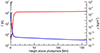 |
Fig. 1. Combined profile of the temperature (solid red line) and density (solid blue line) in hydrostatic equilibrium from the solar interior to the corona, adapted from Bourdin (2014). |
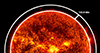 |
Fig. 2. Physical simulation domain spanning the region of the solar atmosphere (located in between the two white circles) from the photosphere to the upper corona, which is 163.8 Mm in height. [Image: NASA/SDO]. |
Simulation setup and grid distances.
As physical model parameters, we used a kinematic viscosity of ν = 109 m2/s and a heat conduction, χ, in the range 5 × 10⁶ − 1010 m2/s. We included radiative losses from Cook et al. (1989) in the energy balance, using photospheric and coronal abundances from Meyer (1985).
We also used so-called Newton cooling to stabilise the temperature and density stratification in the chromosphere and lower TR. Newton cooling is a method that acts similarly to radiative transfer in a non-transparent solar atmosphere but with much less computational demands.
A strong velocity damping is added in the first part of the model evolution in order to reduce the amplitude of the initial settling motions. This damping coefficient will fade out smoothly to zero after approximately 5 h time. The chosen damping coefficient balances the need for stabilisation without suppressing the settling motions entirely. Excessive damping does not lead to better results because the settling motions are then simply suppressed and the perturbation is delayed until the damping vanishes. While too little damping would not suppress the settling motions sufficiently, leading to a crash of the simulation run. Thus, finding the optimal damping is crucial and has been carefully adapted. Those simulations that are stable, evolve and remain stable for at least 24 h.
3.5. Artificial heating function
In a 3D-MHD simulation, the field-line braiding in the photosphere leads to subsequent heating in the corona. Of course, our pure 1D-HD model lacks this self-consistent coronal heating process. Therefore, we included an artificial heating function that acts at all times and depends on the height above the photosphere. This heating function mimics the heat input through realistic coronal heating mechanisms.
To obtain our artificial heating function, we computed the sum of all coronal energy loss terms and smoothed the result with a Gaussian convolution (see the dotted black line in Fig. 3). We flipped the sign of the smoothed energy losses, which then gives us the function we used to replenish the coronal energy from its natural energy losses. Mainly, these coronal energy losses consist of the radiative losses of the coronal plasma plus the heat-conduction terms, which both act as a coronal energy sink.
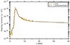 |
Fig. 3. Vertical profile of our artificial heating function. The solid yellow line denotes the sum of all coronal energy loss terms, computed from the initial atmospheric stratification. The dotted black line shows a Gaussian-convolution smoothing applied to the initial energy losses. |
We implemented the heating function in two approaches: heating per volume and heating per particle. Based on our results, we conclude that the heating per particle approach fits our needs better because it is independent of the density stratification. The heating per volume approach shows unwanted runaway effects, where a diminishing density leads to a stronger heating per particle. The plasma packet heats up more, wants to expand adiabatically, and therefore becomes even less dense. This recursive behavioural pattern continues until the temperature explodes to unrealistic values of 109 K and more. As a consequence, the heat conduction implies an extremely short simulation time step, which in practice leads to a stuck simulation run because the time advance per computation cycle is way too low to finish the run in a reasonable time. The mathematical formulation of our heating function, fheat, is
 (5)
(5)
Here, fheat is the energy lost per unit time and per particle. We used lnT in place of the entropy, cP and cV are the specific heat at constant pressure and volume, respectively, γ = cp/cV is the adiabatic index, and nρ denotes the initial particle density. We used here only the initial nρ because we wanted to settle our atmospheric stratification around the expected coronal heating stratification. The reason is that if we transfer our resulting settled atmosphere into a self-consistent 3D-MHD model, we may need to still employ the same artificial heating to prevent the model corona from collapsing due to insufficient heating. Finally, once the 3D-MHD model evolves away from the initial condition, this artificial heating can safely fade out with time, while the self-consistent coronal heating may take over.
4. Results
In explicit numerical schemes, the time step can vary and is adapted according to the physical processes involved. We find an average time step of 0.025 s during our simulation, which is somewhere in between what Bradshaw & Cargill (2013), Reid et al. (2021), and others reported. Of course, the time step depends on the used diffusion parameters and the grid spacing, too. Therefore, we expect different results between other works and ours. In particular, for high-resolution 3D MHD models that include the Spitzer-type heat conduction, one should rather expect time steps of about 1−4 μs.
The 1D-HD simulation evolves away from the initial condition, which is the atmospheric stratification that we show in Fig. 1. With increasing time, we notice that the steep temperature gradient at the TR slowly increases, together with a growth of the temperature at the base of the corona. This growth continues further and develops into a peak in the temperature at heights of about 5−7 Mm (see the upper panel of Fig. 4).
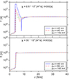 |
Fig. 4. Temperature profiles for three different grid resolutions and two different heat-conduction coefficients, χ. The solid blue lines show a grid distance of 40 km, dashed red lines 80 km, and dotted green lines 160 km. The horizontal axes indicate the atmospheric height, z. The upper panel shows the results for heat conduction of χ = 0.5 × 10⁸ m2/s, and the lower panel χ = 30 × 108 m2/s. |
One might think the rise of the temperature at the base of the corona would have to do with our artificial heating function. Therefore, we tried to reduce the heating around the base of the corona, but we found this did not resolve the issue with the further increasing temperature peak. Since the simulation will eventually crash due to extreme values of temperature and temperature gradients that cannot be numerically resolved, a solution to this issue is necessary, especially because we want to get close to a stable temperature stratification.
We investigate now the effect of three important parameters: (1) the grid resolution, (2) the heat conduction coefficient, and (3) the order of accuracy of the derivative scheme. All other model parameters remain the same for all runs. To assess the effect of the changing parameters, we looked at the maximum temperature in the domain max(T), as well as the maximum of the absolute value of the temperature gradient max(∇T).
We also verified that the influence of hyper-diffusion does not change our results significantly. If a numerical instability occurs and grows, the further time evolution of this instability is mostly unaffected by the amount of hyper-diffusion.
4.1. Grid resolution effects
To investigate the effect of the grid resolution, we performed three identical sets of runs with grid distances of Δz = 160 km, 80 km, and 40 km. In Fig. 4 we show how the temperature profiles develop for each grid resolution (colour coding) at the same physical time t = 300 s in the simulation, just with varying the heat conduction χ for the top panel(χ = 0.5 × 10⁸ m2/s) and bottom panel(χ = 30 × 108 m2/s).
From Fig. 4 we see that the grid resolution has an important influence on multiple aspects of our 1D-HD simulation: First, it is clear that smaller grid distances allow us to model steeper temperature gradients in the TR. We infer this from the slopes of the temperature below z = 5 Mm, where the slopes increase for decreasing grid distances; visible in the upper panels of Figs. 4 and 5.
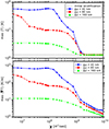 |
Fig. 5. Parametric study for χ vs maximum temperature (above) and χ vs the gradient of maximum temperature (below) for three different resolutions. In both plots, each triangle in the dotted green line represents the runs with a grid distance of 160 km, dots in the dashed red line 80 km, and diamonds in the solid blue line 40 km. The maximum temperature and the gradient of maximum temperature have been taken at 300 seconds for all the runs. The dotted grey line shows the maximum temperature for the reference atmospheric stratification, which is the same for all the runs. The x-axis shows the χ parameter over a range of five orders of magnitude. |
Second, being able to resolve steeper temperature gradients does not necessarily mean that the model becomes more realistic. In practice, we observe that for the same physical heat conduction (χ = 0.5 × 10⁸ m2/s) there develops an unrealistic temperature peak with far over 20 MK for Δz = 40 km and only slightly over 1 MK for the resolution of 160 km. This is of course a purely numerical phenomenon, as the coronal energy loss and heating function are the same across all runs. The reason for this effect is that larger slopes in simulation data put a larger burden on numerical schemes to reproduce the numerical derivatives close to the analytical ones. We see here how this still works for Δz = 160 km but how the same numerical scheme fails for resolutions of 80 km and below.
Third, we find that the remedy to this problem is larger diffusion coefficients in our differential equation system. In particular, a larger heat conduction coefficient (χ = 30 × 108 m2/s) results in again very similar temperature profiles across all tested grid distances (see the lower panel of Fig. 4). This might look counter-intuitive, as usually in numerical turbulence research one would use lower diffusivities for higher grid resolutions under the assumption that higher grid resolutions allow numerical schemes to resolve gradients better. In some cases, this assumption may not hold because processes in the simulation domain will change the maximum observed gradients. Therefore, we now turn to the heat-conduction coefficient χ that we vary over four orders of magnitude.
4.2. Heat conduction effects
To find the best (or the minimum feasible) heat-conduction coefficient, χ, we investigated how the maximum temperature, max(T), and the maximum absolute temperature gradient, max(∇T), change. These maxima are usually reached at the same location in the simulation domain: at the base of the corona for the temperature and in the TR for the positive temperature gradient.
We studied runs that included only the Spitzer-type heat conduction without the isotropic one and we found they were numerically unstable (similar to Fig. 4, top panel). We obtain stable results only if we add isotropic heat conduction. The reason for this behaviour is that Spitzer heat conduction alone does not have the form of a plain diffusion equation. Instead, it strongly depends on absolute temperature and the direction of the magnetic field. Numerical errors, tough, require a diffusion equation to average out rounding errors and keep discontinuities under control. Hence, the isotropic heat conduction needs to be included in many explicit numerical schemes. Still, Spitzer heat conduction should be included to find more realistic atmospheric stratifications.
Here, Fig. 5 shows our parametric study of χ (i.e. the isotropic heat conduction) while keeping all other parameters and physical terms in our model constant. In the upper panel of Fig. 5, we indicate the maximum temperature max(T) for three grid resolutions (colour coding) versus χ. It becomes evident that for χ = 30 × 108 m2/s all grid resolutions yield a consistent value for the maximum in the temperature. This value also matches the maximum temperature taken from our reference initial condition (grey horizontal line in the plot). For any χ below that critical value, we find that the numerical schemes lack enough diffusivity to provide consistent results, leading to unrealistically high temperatures well above 50 MK for the highest grid resolution.
The lower panel of Fig. 5 displays the maximum temperature gradient max(∇T). Again we see, on the one hand, that the simulations follow different trends and even have different slopes in a double-logarithmic plot for heat-conduction coefficients of χ ≤ 30 × 108 m2/s. While, on the other hand, for χ ≥ 30 × 108 m2/s the three different grid resolutions yield at least the same slope in their trend. Still, the maximum gradient of the temperature is different for different grid resolutions. But this is also expected because for lower resolutions the maximum possible gradients of any quantity are in general lower (see the roughly constant offsets between the blue, red, and green data points in the lower panel of Fig. 5 for χ ≥ 30 × 108 m2/s).
4.3. Order of derivative scheme
We turn to a comparison of second-, fourth-, sixth-, eighth-, and tenth-order accuracy for derivatives, now implementing the fourth-order scheme in the Pencil Code.
Fig. 6 depicts how the maximum temperature (top panel) and the maximum gradient of temperature (bottom panel) vary with the heat conduction coefficient and different orders of the numerical scheme used. For higher chi values all numerical schemes seem to perform the same and show expected 106 temperatures in the solar corona. For χ ≤ 108 m2/s, there are discrepancies between the schemes. For example, the peak temperature (top panel) of the lowest-order scheme is about 25% higher, as compared to the highest order. Similarly, the temperature gradient also differs more for low χ values, which indicates stronger numerical difficulties.
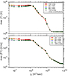 |
Fig. 6. Parametric study for χ vs maximum temperature (above) and χ vs the gradient of maximum temperature (below) for different orders of the numerical scheme. In both plots, each marker corresponds to a numerical scheme: red circles (solid line) represent the second-order scheme, orange triangles (solid line) the fourth-order, blue diamonds (dotted line) the sixth-order, green stars (dotted line) the eighth-order, and black crosses (dotted line) the tenth-order. The x-axis shows the χ parameter over a range of five orders of magnitude. The maximum temperature and the gradient of maximum temperature have been taken at 300 seconds for all the runs. The blue diamond markers represent the same data as the blue curve in Fig. 5. |
In Fig. 7 the comparison across the quadrants highlights the effect of the grid resolution and diffusivity over different orders of numerical schemes. For the same grid spacing, lower isotropic diffusion coefficients produce more pronounced numerical instabilities, observed as ‘wiggles’ (see panel a vs c as well as panel b vs d). For the same diffusion coefficient, a finer grid spacing resolves the temperature gradients better (see panel a vs b, as well as panel c vs d). From panel c we conclude that combining high diffusivity with smaller grid spacing gives consistently more realistic results for all accuracy orders of the numerical schemes because the simulation result is closest to the expected result.
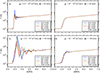 |
Fig. 7. Temperature profiles of different order numerical schemes for varying heat-conduction coefficients, χ, and grid resolutions, Δz, at the same physical time, t = 300 s, in the simulation. The horizontal axes indicate the atmospheric height, z. The solid blue line represents the run with the second-order numerical scheme, the dashed green and orange lines the fourth- and the eighth-order runs, respectively, and the dotted black lines the tenth-order runs. The solid red line represents the sixth-order derivative numerical scheme, which was the chosen numerical scheme for our simulation. Panels c and d show the results for a heat conduction of χ = 30 − 108 m2/s, and panels a and d the results for a heat conduction of χ = 0.5 − 108 m2/s. |
For the same grid distances, here Δz = 40 km and Δz = 160 km, the lowest-order schemes produce the least realistic time evolution of the model than compared to the highest-order scheme (see the consecutively higher amplitudes of the wiggles from the tenth order to the second order in Fig. 7, panels a and b). We find that the amplitude of the wiggles is largest for the lowest order on the same grid spacing. Implicitly, to achieve the same amplitudes for the wiggles, the low-order schemes require smaller grid distances as compared to the high-order schemes. This ultimately means that low-order schemes might have an advantage because the computation of derivatives can be done faster by using smaller stencils, while for the same physical accuracy, more grid points are needed for the same spatial domain, which again increases the computational demands.
When we look at panel b of Fig. 7 we notice that the wiggles feature different spatial frequencies, where the frequency decreases with the order of the scheme. The main peak for all orders is located at z = 4.7 Mm. From there, we searched for the location of the second minimum of the wiggles. For the tenth order, the second minimum occurs at z = 5.2 Mm, for the sixth order at 5.3 Mm, and for the second order it is located around z = 5.5 Mm.
5. Conclusions
For HD and MHD simulations, an educated guess of the diffusivities is crucial for obtaining numerical stability and to come close to physical realism. We performed a parameter study of a 1D-HD model of a vertical solar-atmospheric column. We find that for grid resolutions from Δz = 40 km to 160 km, a heat-conduction coefficient of χ = 30 × 108 m2/s is the optimal choice to maintain realistic temperature profiles under realistic coronal heating and cooling terms. Contrary to the widespread idea of using less diffusivity for smaller grid distances, we find that larger χ values are needed to stabilise the numerical scheme and maintain control of the steep temperature gradients in the TR.
From Fig. 6 we conclude that the order of the derivative scheme would not significantly change the time evolution of the development of numerical instabilities. For χ ≥ 108 m2/s, we find asymptotic behaviour (see the top and bottom panels as well as panel c of Fig. 7).
The artificial heating function we used in the corona to compensate for the realistic energy losses is able to maintain and stabilise the expected coronal temperature stratification. We find that with our choice of χ = 30 × 108 m2/s, our three different grid resolutions yield about the same temperature stratification. Even though the maximum temperature gradient systematically depends on the grid resolution, it shows the same trend when χ varies.
For this study, 1D-HD simulations were sufficient to study the effect of the heat conduction because we included a coronal heating function that mimics the effects of 3D magnetic-field perturbations leading to Ohmic current dissipation in the corona. In future work, we will investigate the effect of magnetic pressure, which may partly compensate for the gravitational pull on the plasma. This will allow us to include the widely used Spitzer heat conduction, which is aligned with the magnetic field and is proportional to T5/2. A combination of both Spitzer-type and isotropic heat conduction might give the best results for numerical stability. We anticipate this will be necessary to prepare the atmospheric stratification to be usable in MHD simulations.
Using higher diffusivities together with lower grid resolutions, in combination with high-order derivatives in explicit numerical schemes, allows us to achieve larger time steps. At the same time, the total number of grid points is drastically reduced, especially for 3D simulations. In total, this gives more benefits than drawbacks. For example, instead of a 40−100 km grid spacing, if we use low-order derivatives with less diffusivity, we would need about 1−10 km to maintain the same level of physical detail. Such high grid resolutions are not feasible for large 3D simulations in the foreseeable future.
Our resulting atmospheric temperature stratification can serve as initial conditions for larger models with higher dimensionality or for spectro-polarimetric inversions, where temperature stratifications are required input.
Acknowledgments
We thank the anonymous referee for valuable input to improve the manuscript. This research was funded in whole or in part by the Austrian Science Fund (FWF) [10.55776/P32958] and [10.55776/P37265].
References
- Bingert, S., & Peter, H. 2011, A&A, 530, A112 [NASA ADS] [CrossRef] [EDP Sciences] [Google Scholar]
- Bourdin, P.-A. 2014, Cent. Eur. Astrophys. Bull., 38, 1 [Google Scholar]
- Bourdin, P.-A. 2017, An. Geo., 35, 1051 [NASA ADS] [CrossRef] [Google Scholar]
- Bourdin, P.-A. 2020, Geophys. Astrophys. Fluid Dyn., 114, 235 [NASA ADS] [CrossRef] [Google Scholar]
- Bradshaw, S. J., & Cargill, P. J. 2013, ApJ, 770, 12 [NASA ADS] [CrossRef] [Google Scholar]
- Cook, J. W., Cheng, C.-C., Jacobs, V. L., & Antiochos, S. K. 1989, ApJ, 338, 1176 [Google Scholar]
- Fontenla, J. M., Avrett, E. H., & Loeser, R. 1993, ApJ, 406, 319 [Google Scholar]
- Gudiksen, B., & Nordlund, Å. 2002, ApJ, 572, L113 [NASA ADS] [CrossRef] [Google Scholar]
- Hori, K., Yokoyama, T., Kosugi, T., & Shibata, K. 1997, ApJ, 489, 426 [NASA ADS] [CrossRef] [Google Scholar]
- Howson, T. A., & Breu, C. 2023, MNRAS, 526, 499 [NASA ADS] [CrossRef] [Google Scholar]
- Johnston, C. D., Cargill, P. J., Antolin, P., et al. 2019, A&A, 625, A149 [NASA ADS] [CrossRef] [EDP Sciences] [Google Scholar]
- Klimchuk, J. A. 2006, Sol. Phys., 234, 41 [Google Scholar]
- Kowalski, A. F., Hawley, S. L., Carlsson, M., et al. 2015, Sol. Phys., 290, 3487 [NASA ADS] [CrossRef] [Google Scholar]
- Lionello, R., Downs, C., Linker, J. A., et al. 2019, Sol. Phys., 294, 13 [NASA ADS] [CrossRef] [Google Scholar]
- MacNeice, P. 1986, Sol. Phys., 103, 47 [NASA ADS] [CrossRef] [Google Scholar]
- McClymont, A. N., & Craig, I. J. D. 1982, BAAS, 14, 900 [NASA ADS] [Google Scholar]
- McIntosh, S. W., de Pontieu, B., Carlsson, M., et al. 2011, Nature, 475, 477 [Google Scholar]
- Meyer, J.-P. 1985, ApJS, 57, 173 [Google Scholar]
- Müller, D., Hansteen, V. H., & Peter, H. 2003, A&A, 411, 605 [NASA ADS] [CrossRef] [EDP Sciences] [Google Scholar]
- Müller, D., De Groof, A., Hansteen, V. H., & Peter, H. 2005, A&A, 436, 1067 [NASA ADS] [CrossRef] [EDP Sciences] [Google Scholar]
- November, L. J., & Koutchmy, S. 1996, ApJ, 466, 512 [CrossRef] [Google Scholar]
- Parker, E. N. 1972, ApJ, 174, 499 [NASA ADS] [CrossRef] [Google Scholar]
- Pencil Code Collaboration (Brandenburg, A., et al.) 2021, J. Open Source Softw., 6, 2807 [Google Scholar]
- Reid, J., Cargill, P. J., Johnston, C. D., & Hood, A. W. 2021, MNRAS, 505, 4141 [NASA ADS] [CrossRef] [Google Scholar]
- Solanki, S. K., Lagg, A., Woch, J., Krupp, N., & Collados, M. 2003, Nature, 425, 692 [Google Scholar]
- Stix, M. 2004, The Sun. An Introduction (Berlin: Springer) [Google Scholar]
- Vernazza, J. E., Avrett, E. H., & Loeser, R. 1981, ApJS, 45, 635 [Google Scholar]
- Warren, H. P. 2006, ApJ, 637, 522 [NASA ADS] [CrossRef] [Google Scholar]
All Tables
All Figures
|
Fig. 1. Combined profile of the temperature (solid red line) and density (solid blue line) in hydrostatic equilibrium from the solar interior to the corona, adapted from Bourdin (2014). |
| In the text | |
|
Fig. 2. Physical simulation domain spanning the region of the solar atmosphere (located in between the two white circles) from the photosphere to the upper corona, which is 163.8 Mm in height. [Image: NASA/SDO]. |
| In the text | |
|
Fig. 3. Vertical profile of our artificial heating function. The solid yellow line denotes the sum of all coronal energy loss terms, computed from the initial atmospheric stratification. The dotted black line shows a Gaussian-convolution smoothing applied to the initial energy losses. |
| In the text | |
|
Fig. 4. Temperature profiles for three different grid resolutions and two different heat-conduction coefficients, χ. The solid blue lines show a grid distance of 40 km, dashed red lines 80 km, and dotted green lines 160 km. The horizontal axes indicate the atmospheric height, z. The upper panel shows the results for heat conduction of χ = 0.5 × 10⁸ m2/s, and the lower panel χ = 30 × 108 m2/s. |
| In the text | |
|
Fig. 5. Parametric study for χ vs maximum temperature (above) and χ vs the gradient of maximum temperature (below) for three different resolutions. In both plots, each triangle in the dotted green line represents the runs with a grid distance of 160 km, dots in the dashed red line 80 km, and diamonds in the solid blue line 40 km. The maximum temperature and the gradient of maximum temperature have been taken at 300 seconds for all the runs. The dotted grey line shows the maximum temperature for the reference atmospheric stratification, which is the same for all the runs. The x-axis shows the χ parameter over a range of five orders of magnitude. |
| In the text | |
|
Fig. 6. Parametric study for χ vs maximum temperature (above) and χ vs the gradient of maximum temperature (below) for different orders of the numerical scheme. In both plots, each marker corresponds to a numerical scheme: red circles (solid line) represent the second-order scheme, orange triangles (solid line) the fourth-order, blue diamonds (dotted line) the sixth-order, green stars (dotted line) the eighth-order, and black crosses (dotted line) the tenth-order. The x-axis shows the χ parameter over a range of five orders of magnitude. The maximum temperature and the gradient of maximum temperature have been taken at 300 seconds for all the runs. The blue diamond markers represent the same data as the blue curve in Fig. 5. |
| In the text | |
|
Fig. 7. Temperature profiles of different order numerical schemes for varying heat-conduction coefficients, χ, and grid resolutions, Δz, at the same physical time, t = 300 s, in the simulation. The horizontal axes indicate the atmospheric height, z. The solid blue line represents the run with the second-order numerical scheme, the dashed green and orange lines the fourth- and the eighth-order runs, respectively, and the dotted black lines the tenth-order runs. The solid red line represents the sixth-order derivative numerical scheme, which was the chosen numerical scheme for our simulation. Panels c and d show the results for a heat conduction of χ = 30 − 108 m2/s, and panels a and d the results for a heat conduction of χ = 0.5 − 108 m2/s. |
| In the text | |
Current usage metrics show cumulative count of Article Views (full-text article views including HTML views, PDF and ePub downloads, according to the available data) and Abstracts Views on Vision4Press platform.
Data correspond to usage on the plateform after 2015. The current usage metrics is available 48-96 hours after online publication and is updated daily on week days.
Initial download of the metrics may take a while.