| Issue |
A&A
Volume 692, December 2024
|
|
|---|---|---|
| Article Number | A175 | |
| Number of page(s) | 17 | |
| Section | Cosmology (including clusters of galaxies) | |
| DOI | https://doi.org/10.1051/0004-6361/202451286 | |
| Published online | 12 December 2024 | |
CLASH-VLT: Galaxy cluster MACS J0329–0211 and its surroundings using galaxies as kinematic tracers
1
Dipartimento di Fisica dell’Università degli Studi di Trieste – Sezione di Astronomia, Via Tiepolo 11, I-34143 Trieste, Italy
2
INAF – Osservatorio Astronomico di Trieste, Via Tiepolo 11, I-34143 Trieste, Italy
3
Fundación Galileo Galilei – INAF (Telescopio Nazionale Galileo), Rambla José Ana Fernández Perez 7, E-38712 Breña Baja (La Palma), Canary Islands, Spain
4
Instituto de Astrofísica de Canarias, C/Vía Láctea s/n, E-38205 La Laguna (Tenerife), Canary Islands, Spain
5
Departamento de Astrofísica, Univ. de La Laguna, Av. del Astrofísico Francisco Sánchez s/n, E-38205 La Laguna (Tenerife), Spain
6
Dipartimento di Fisica E. R. Caianiello, Università Degli Studi di Salerno, Via Giovanni Paolo II, I-84084 Fisciano, (SA), Italy
7
INAF – Osservatorio Astronomico di Capodimonte, Via Moiariello 16, I-80131 Napoli, Italy
8
Dipartimento di Fisica e Scienze della Terra, Università di Ferrara, Via Saragat 1, 44122 Ferrara, Italy
9
INAF – Osservatorio di Astrofisica e Scienza dello Spazio di Bologna, Via Gobetti 93/3, 40129 Bologna, Italy
10
IFPU – Institute for Fundamental Physics of the Universe, Via Beirut 2, 34014 Trieste, Italy
11
Institute of Astrophysics, Facultad de Ciencias Exactas, Universidad Andrés Bello, Sede Concepción, Talcahuano, Chile
12
Dipartimento di Fisica, Università degli Studi di Milano, Via Celoria 16, 20133 Milano, Italy
13
INAF – IASF Milano, Via A. Corti 12, 20133 Milano, Italy
14
University Observatory, Ludwig-Maximilians University Munich, Scheinerstrasse 1, 81679 Munich, Germany
15
INAF – Osservatorio Astrofisico di Arcetri, Largo E. Fermi, 50125 Firenze, Italy
⋆ Corresponding author; This email address is being protected from spambots. You need JavaScript enabled to view it.
Received:
27
June
2024
Accepted:
24
October
2024
Abstract
Context. The study of substructure is an important step in determining how galaxy clusters form.
Aims. We aim to gain new insights into the controversial dynamical status of MACS J0329–0211 (MACS0329), a massive cluster at z = 0.4503 ± 0.0003, through a new analysis using a large sample of member galaxies as kinematic tracers.
Methods. Our analysis is based on extensive spectroscopic data for more than 1700 galaxies obtained with the VIMOS and MUSE spectrographs at the Very Large Telescope (VLT) in combination with B and RC Suprime-Cam photometry from the Subaru archive. According to our member selection procedure, we defined a sample of 430 MACS0329 galaxies within 6 Mpc, corresponding to approximately three times the virial radius.
Results. We estimated the global velocity dispersion, σV841-36+26 km s−1, and present the velocity dispersion profile. We estimated a mass of M200 = (9.2 ± 1.5)×1014 M⊙ using 227 galaxies within R200 = (1.71 ± 0.07) Mpc, for which σV,200841-48+40 km s−1. The spatial distribution of the red galaxies traces a SE-NW elongated structure without signs of a velocity gradient. This structure likely originates from the main phase of cluster assembly. The distribution of the blue galaxies is less concentrated and more rounded, and it shows signs of substructure, all characteristics indicating a recent infall of groups from the field. We detected two loose clumps of blue galaxies in the south and southwest at a distance of ∼R200 from the cluster center. The strong spatial segregation among galaxy populations is not accompanied by a kinematical difference. Thanks to our extensive catalog of spectroscopic redshift, we were able to study galaxy systems that are intervening along the line of sight. We identified two foreground galaxy systems, GrG1 at z ∼ 0.31 and GrG2 at z ∼ 0.38, and one background system, GrG3 at z ∼ 0.47. We point out that the second brightest galaxy projected onto the MACS0329 core is in fact the dominant galaxy of the foreground group GrG2. MACS0329, GrG3, and two other systems detected using DESI DR9 photometric redshifts are close to each other, suggesting the presence of a large-scale structure.
Conclusions. MACS0329 is close to a state of dynamical equilibrium despite being surrounded by a very rich environment. We emphasize that the use of an extensive spectroscopic redshift survey is essential to avoiding misinterpretation of structures projected along the line of sight.
Key words: galaxies: clusters: general / galaxies: clusters: individual: MACS J0329–0211 / galaxies: kinematics and dynamics
We dedicate this paper to the memory of our friend and colleague Mario.
© The Authors 2024
 Open Access article, published by EDP Sciences, under the terms of the Creative Commons Attribution License (https://creativecommons.org/licenses/by/4.0), which permits unrestricted use, distribution, and reproduction in any medium, provided the original work is properly cited.
This article is published in open access under the Subscribe to Open model. This email address is being protected from spambots. You need JavaScript enabled to view it. to support open access publication.
1. Introduction
In the context of cold dark matter ΛCDM cosmology, numerical simulations show that structure formation takes place hierarchically and culminates in the formation of galaxy clusters. Galaxy clusters are preferentially formed by anisotropic accretion along the large-scale structure filaments and to a considerable extent by the accretion of galaxy groups, whereas the merger of two or more massive entities is a rare case (e.g., Berrier et al. 2009; McGee et al. 2009). Clusters are multicomponent systems, and merger and accretion phenomena are detected using multiwavelength observations and a variety of techniques focusing on the different components, mainly dark matter, the hot intracluster medium (ICM), and galaxies (see Feretti et al. 2002; Molnar 2016).
The use of multiband optical data, and in particular multiobject spectroscopy, is a consolidated method to study the overall structure and substructures of galaxy clusters and cluster-merging phenomena. This information complements X-ray information since it is known that galaxies and the ICM react on different timescales during a merger, as shown by numerical simulations (e.g., Roettiger et al. 1997; Springel & Farrar 2007; McDonald et al. 2022) and observational data (e.g., the Bullett cluster; Markevitch 2006). Nearly collisionless dark matter and galaxies are expected to take longer to reach the dynamical equilibrium state than the collisional ICM (e.g., Poole et al. 2006).
Since formation history varies greatly from cluster to cluster (e.g., Berrier et al. 2009), most observational studies focus on individual systems. Very large spectroscopic datasets are needed to study clusters in projected phase space for different galaxy types and to infer the formation history, as has been shown for a few clusters where spectroscopic information is available for hundreds of members (e.g., Czoske et al. 2002; Rines et al. 2003; Demarco et al. 2010; Owers et al. 2011; Munari et al. 2014; Girardi et al. 2015; Sohn et al. 2019; Mercurio et al. 2021).
The object of this study, the galaxy cluster MACS J0329−0211 (hereafter MACS0329) at z ∼ 0.45, owes its name to its inclusion in the Massive Cluster Survey (MACS; Ebeling et al. 2001). It is also listed as an extended source in the ROSAT All-Sky Survey Bright Source Catalog (RASS-BSC; Voges et al. 1999). MACS0329 is a fairly X-ray bright (LX, bol = 17 × 1044 erg s−1; Postman et al. 2012) hot (TX ∼ 7 − 8 keV, Cavagnolo et al. 2008; Postman et al. 2012) and massive cluster with M2001 in the range of 7 − 13 × 1014 M⊙ (Schmidt & Allen 2007; Donahue et al. 2014; Umetsu et al. 2014, 2016, 2018; Merten et al. 2015; Herbonnet et al. 2019).
Notably, MACS0329 was also part of the project Cluster Lensing and Supernova Survey with Hubble (CLASH; Postman et al. 2012). The CLASH X-ray selection favors the inclusion of highly relaxed clusters, and indeed the X-ray image of MACS0329 is unimodal (e.g., Yuan & Han 20202; see also our Fig. 1). Postman et al. (2012) referred to MACS0329 as one of the eight CLASH clusters with a possible substructure. Indeed, MACS0329 was classified as dynamically relaxed by some authors at the time (Schmidt & Allen 2007; Allen et al. 2008), but Maughan et al. (2008) reported evidence for a substructure. More recent results are also controversial and suggest either a relaxed (e.g., Mann & Ebeling 2012; Yuan & Han 2020) or a non-relaxed cluster (e.g., Sayers et al. 2013; Mantz et al. 2015). MACS0329 shows a bright cool core with low entropy (e.g., Cavagnolo et al. 2008; Sayers et al. 2013), which is to be expected for a relaxed galaxy cluster. However, when analyzing the central regions, Ueda et al. (2020) found a spiral-like pattern in the X-ray residual image that is consistent with a gas sloshing in the core, which is likely related to an infalling subcluster. Embedded in the cool core is the brightest cluster galaxy (BCG) with very high UV emission and a very high star formation rate (Donahue et al. 2015; Fogarty et al. 2015) as well as a blue color and strong optical emission lines (Green et al. 2016). The BCG also shows radio emission, which is likely due to an active galactic nucleus (AGN; Yu et al. 2018). In addition, Giacintucci et al. (2014, 2019) have detected a radio mini-halo, a phenomenon that only occurs in cool-core clusters and is likely related to gas sloshing and AGN feedback (e.g., Richard-Laferrière et al. 2020). Finally, there is a second giant elliptical galaxy 40″ northwest of the BCG, which stimulated the idea that MACS0329 could be undergoing a merger event (e.g., Caminha et al. 2019). Indeed, DeMaio et al. (2015) analyzed the diffuse intracluster light surrounding the BCG and concluded that the two galaxies have already interacted with each other.
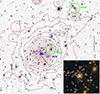 |
Fig. 1. Suprime-Cam RC-band image (north top and east left) of the MACS0329 field with superimposed isocontour levels of the Chandra X-ray emission (energy range: 0.5−7 keV). Only the main cluster region is shown. Small blue circles mark cluster members (see Sect. 3). The blue label indicates the brightest cluster galaxy. Green labels and large circles indicate the two foreground groups (GrG1 at z = 0.314 and GrG2 at z = 0.385) projected onto the field of the cluster (see Sect. 7). The inset shows a color composite image of the central region (1.5 × 1.5 arcmin2) from the CLASH survey (Postman et al. 2012), which combines HST/ACS and WFC3 passbands. Member galaxies of MAC0329 and GrG2 are indicated by circles and squares, respectively (large symbols indicate the two brightest members of MACS0329 and GrG2). |
The above extensive bibliography shows the great interest in MACS0329 and the controversial evidence for its substructure. To date, however, there is no study based on the kinematics of the member galaxies. MACS0329 is part of the ESO Large Program Dark Matter Mass Distributions of Hubble Treasury Clusters and the Foundations of ΛCDM Structure Formation Models, which aims to obtain the panoramic spectroscopic survey of the 13 CLASH clusters visible from ESO-Paranal, also known as the CLASH-VLT3 campaign (Rosati et al. 2014), based on data obtained at the Very Large Telescope (VLT).
This article is organized as follows. We describe our data and the selection of member galaxies in Sects. 2 and 3. Sections 4, 5, and 6 deal with the structure of MACS0329, that is its main properties, the galaxy population, and the substructure. Other galaxy systems projected onto the field of MACS0329 or in its vicinity are analyzed in Sect. 7. Section 8 is devoted to the interpretation and discussion of our results. Our summary and conclusions can be found in Sect. 9.
In this work we use H0 = 70 km s−1 Mpc−1 in a flat cosmology with Ω0 = 0.3 and ΩΛ = 0.7. In the assumed cosmology, 1′∼346 kpc at the redshift of MACS0329. All magnitudes are given in the AB system. The velocities we derive for the galaxies are line-of-sight velocities determined from the redshift, V = cz. Unless otherwise stated, we report the errors with a confidence level (c.l.) of 68%.
2. Data and galaxy catalog
The spectroscopic catalog of MACS0329 here considered consists of 1712 galaxies with a redshift between 0 and 1. We exploited an extensive spectroscopic campaign of the MACS0329 field with the VIMOS spectrograph (VIsible MultiObject Spectrograph), as part of the CLASH-VLT Large Program (Rosati et al. 2014), augmented with MUSE integral field spectroscopy in the cluster core. For the full catalog we refer to Rosati et al. (in prep.). VLT-VIMOS data were reduced with the VIPGI package (Scodeggio et al. 2005), details can be found in Mercurio et al. (2021). Each redshift was assigned a quality flag. In this work, only VIMOS redshifts with a quality flag QF = 3 (secure) and QF = 2 were considered, the latter refer to redshifts with a reliability ≳80%. The reliability of the quality flags is assessed on the basis of duplicate observations with at least one secure measurement, as described in Balestra et al. (2016). Details about VLT-MUSE data can be found in Caminha et al. (2019). When both VIMOS and MUSE redshifts are available, we only considered the MUSE measurement. A MUSE redshift measurement is available for the brightest cluster galaxy. In this study, all MUSE and VIMOS galaxies with a redshift between 0 and 1 have been considered, giving a total of 74 and 1637 redshifts, respectively. The VIMOS data provide us with an efficient coverage of an important cluster volume sampling MACS0329 out to a radius R ≳ 3 R200. The MUSE data allowed us to sample the central ≲2′ region, which could not be adequately sampled by standard multislit spectroscopy.
We also obtained two long-slit spectra for the very bright galaxy ∼40″ northwest of the BCG [at RA =  , Dec = −02° 11′29.2″ (J2000.0)]. In Sect. 7, we show that this galaxy, the second brightest galaxy projected onto the cluster core, is in fact the dominant galaxy of a foreground group (GrG2; see Sect. 7). This galaxy was observed with the Italian Telescopio Galileo (TNG) with a total exposure time of 3600 s in 2018 (see Fig. 2).
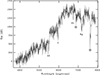 |
Fig. 2. Spectrum from TNG of the brightest galaxy of the foreground GrG2 group (z = 0.385), which is projected ∼40″ to the northwest of the center of MACS0329 (see Fig. 1). The x-axis shows the rest-frame wavelength. The main spectral features are marked by their symbols. The two telluric features at ∼6900 Å and 7600 Å are also shown (marked by the earth symbol). |
For the MACS0329 field, we used photometric information from Suprime-Cam data. The images were retrieved from the CLASH page4 available at the Mikulski Archive for Space Telescopes (MAST). A full description of the reduction of the Suprime-Cam images can be found in the data section of the CLASH website5. Briefly, the images were reduced by one of us using the techniques described in Nonino et al. (2009) and Medezinski et al. (2013). The total area covered by the images is 34′×27′. The zeropoints are in the AB system. Specifically, we retrieved the image in the RC-band with an exposure time of 2400 s and a depth of 26.5 mag, and the image in the B-band with an exposure of 2940 s and a depth of 27.2 mag. The photometric catalogs were produced using the software SExtractor (Bertin & Arnouts 1996). We extracted independent catalogs in each band that were then matched across the wavebands using STILTS (Starlink Tables Infrastructure Library Tool Set, Taylor 2006). Among the photometric quantities, we measured aperture magnitudes (MAG_APER) in circular apertures with diameters of 5.0 arcsec and we estimated the Kron magnitude (MAG_AUTO) through an adaptive elliptical aperture (Kron 1980). Unless otherwise stated, the values listed are dereddened magnitudes; that is, we applied the correction for Galactic extinction.
We were able to assign magnitudes to 1693 out of 1712 galaxies in the redshift catalog. This catalog is electronically published in Table 1, available at the Strasbourg astronomical Data Center (CDS). VIMOS was used with both the low-resolution blue grism (LRb) and the medium-resolution grism (MR) with typical uncertainties of cz = 150 and 75 km s−1, respectively (Biviano et al. 2013; Balestra et al. 2016). Typical uncertainties of MUSE redshifts are cz = 40 km s−1 (Inami et al. 2017). For the TNG redshift, the uncertainty is cz = 100 km s−1.
Spectroscopic redshift catalog (extract).
3. Member selection
To select cluster members from the 1712 galaxies with redshifts, we applied the two-step method known as “peak +gap” (P+G), which has already been used for CLASH-VLT clusters (e.g., Girardi et al. 2015). In the first step, we analyzed the redshift sample using the 1D adaptive-kernel method of Pisani (1993, hereafter DEDICA). Using this method, MACS0329 is identified as a peak at z = 0.4504 populated by 533 galaxies (in the range 0.4333 ≤ z ≤ 0.4664, see Fig. 3).
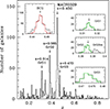 |
Fig. 3. Distribution of galaxy redshifts. The histogram refers to the galaxies with the spectroscopic redshift in the region of MACS0329 with 0.1 < z < 0.9. Labels indicate redshifts of the relevant peaks and the names of the corresponding galaxy systems, that is MACS0329 and other groups (see Table 2). The redshift distribution of the 533 galaxies assigned to the MACS0329 peak can be seen in the inset plot at the top left (black line histogram). The histogram with the red line refers to the 430 galaxies that are members. The BCG redshift is also shown. For each of the other groups, the respective right-hand inset panel shows the redshift distribution of the galaxies assigned to the peak and the galaxies selected as members (black and green line histograms, respectively, see Sect. 7). For GrG1 and GrG2, the arrows indicate the redshifts of the luminous galaxies that we have selected as the centers of the groups. |
The redshift space around MACS0329 is particularly rich in structures, and Table 2 lists all peaks with a relative density with respect to the densest peak, ρ > 0.25. These densest peaks are associated with other galaxy systems and will be investigated in Sect. 7.
Peaks in the redshift distribution.
In the second step, we combined the spatial and velocity information which works in projected phase space. In fact, galaxies in clusters appear within regions delimited by caustics with a characteristic trumpet shape (Kaiser 1987; Regos & Geller 1989) and outside the caustics the density of galaxies drops substantially (see Fig. 5 for MACS0329). Galaxies outside the caustics are background or foreground galaxies (e.g., den Hartog & Katgert 1996; Diaferio & Geller 1997; Geller et al. 1999). We applied the “shifting gapper” method (Fadda et al. 1996; Girardi et al. 1996). Of the galaxies that lie within an annulus around the center of the system, the method excludes those that are too far away in velocity from the main body of galaxies, that is further than a certain velocity distance called the velocity gap. The position of the annulus is shifted with increasing distance from the center of the cluster. The procedure is repeated until the number of cluster members converges to a stable value. We defined the center of the cluster as the position in RA and Dec of the BCG. The BCG lies at the center of the main galaxy peak in the 2D spatial galaxy distribution (see Sect. 6.2 and Fig. 4). Following Fadda et al. (1996), we chose an annulus size of 0.6 Mpc or more to include at least 15 galaxies. For the velocity gap they suggested a value of 1000 km s−1, but smaller values are more appropriate for deeply sampled clusters as in the case of CLASH-VLT (e.g., 800 km s−1 in Girardi et al. 2015 and 500 km s−1 in Balestra et al. 2016).
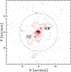 |
Fig. 4. Spatial distribution and isodensity contours of the cluster members with RC ≤ 24 within the 20′×20′ region centered on the BCG, corresponding to ∼7 × 7 Mpc2. Large and small crosses show the position of the BCG and the secondary density peaks (see Table 7). The R200 region is highlighted by the circle. |
The projected phase space around MACS0329 is particularly rich in galaxies (see Fig. 5). When applying different values for the velocity gap, the difference in membership is small in the R200 cluster region, but significant in the outer cluster regions. To better understand the best value for the velocity gap, we analyzed the velocity distribution of 236 galaxies that survived the velocity gap of 800 km s−1 in the region outside 2 Mpc. We used the 1D-Kaye’s Mixture Model test (1D-KMM test; Ashman et al. 1994), which fits a user-defined number of Gaussian distributions to a dataset and evaluates the improvement of this fit compared to a single Gaussian distribution. A three-group partition (18, 180 and 38 galaxies) is significantly better at the > 99.9% c.l. and proves that the cluster is indeed surrounded by galaxies with low and high velocities. We adopted a velocity gap of 500 km s−1, leading to a membership in the outer cluster regions that is very similar to the KMM result, that is differing for six of 180 galaxies. Of the 533 galaxies in the cluster velocity peak, 103 galaxies are discarded by this procedure. In summary, the sample of fiducial cluster members consists of 430 galaxies (hereafter called the TOT sample) of which 421 have complete photometric information.
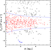 |
Fig. 5. Projected phase space of galaxies in the MACS0329 field with the rest-frame velocity Vrf = (V − ⟨V⟩)/(1 + z) versus the projected cluster-centric distance R. Dots show the 533 galaxies selected in the velocity peak of the cluster according to the 1D-DEDICA method. Red dots indicate the 430 galaxies that are considered true cluster members according to the second step of the member selection. The BCG position is indicated by the box at R = 0. The blue curves contain the region where Vrf is smaller than the escape velocity (see text). |
Figure 5 also shows the escape velocity curves calculated according to den Hartog & Katgert (1996). In particular, we assumed a NFW mass density profile (Navarro, Frenk and White – Navarro et al. 1997) where the concentration parameter is given by Umetsu et al. (2018) and the mass value is estimated in the following section. This is an a posteriori verification of our membership procedure.
4. Global properties of the cluster
We calculated the mean redshift of the 430 cluster galaxies of the TOT sample sample as ⟨z⟩ = 0.4503 ± 0.0003, which corresponds to a mean line-of-sight velocity of ⟨V⟩ = 135 011 ± 40 km s−1, using the biweight estimator (ROSTAT software for robust statistics by Beers et al. 1990). We estimated the velocity dispersion, σV, by applying the cosmological correction and the standard correction for velocity errors (Danese et al. 1980), thus obtaining  km s−1, where errors have been estimated by a bootstrap method.
To derive the mass M200, we used the theoretically expected relation between M200 and the velocity dispersion, which was also verified on simulated clusters (Eq. 1 of Munari et al. 2013) We adopted a recursive approach. To obtain an initial estimate of the radius R200 and M200, we applied the relation of Munari et al. to the global value of σV. We considered the galaxies within this first estimate of R200 to recalculate the velocity dispersion. The procedure is repeated until a stable result is obtained. We estimated  km s−1 for 227 galaxies within R200 = (1.71 ± 0.07) Mpc, and M200 = (9.2 ± 1.5)×1014 M⊙. The uncertainty for R200 has been calculated using the error propagation for σV (R200 ∝ σV) and the uncertainty for M200 has been estimated using a similar error propagation (M200 ∝ σV3) and an additional uncertainty of 10% to account for the scatter around the relation of Munari et al. (2013). In the following, we refer to the 227 galaxies within R200 as the R200 sample. Of these 227 galaxies, 218 have the full magnitude information. The main properties of the cluster are listed in Table 3.
Global properties of MACS0329.
We determined the cluster mass profile, M(r), in two more sophisticated ways, namely using the Modeling Anisotropy and Mass Profiles of Observed Spherical Systems (MAMPOSSt) method of Mamon et al. (2013) and the caustic method of Diaferio & Geller (1997). MAMPOSSt solves the Jeans equation for dynamical equilibrium by performing a maximum likelihood fit of models of cluster mass profile, M(r), and velocity anisotropy profile, β(r), to the distribution of cluster members in the projected phase-space. We chose the NFW model for M(r) and the Tiret model (Tiret et al. 2007) for β(r). We performed the fit to the number density profile of cluster members externally to MAMPOSSt, by considering a NFW profile in projection (Bartelmann 1996). We found a best-fit scale radius for the number density profile  Mpc. We then determined the marginal distributions of the four free parameters of M(r) and β(r) – namely, the virial and scale radii, R200 and rs, the central velocity anisotropy β0 and the asymptotic value at large radii β∞ – using the Markov chain Monte Carlo (MCMC) technique. The resulting M(r) best-fit parameters and 68% marginalized errors are
 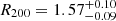 Mpc and
  Mpc, and those of β(r) are
  and
and  , indicating slightly radial orbits for the cluster members.
The caustic method is based on the identification of density discontinuities in the projected phase-space and does not require the assumption of a model for M(r). The amplitude of the caustic in velocity space as a function of radius can be converted to a mass profile, modulo a factor ℱβ. We assumed that ℱβ = 0.5, as recommended by Diaferio & Geller (1997) and Rines et al. (2003, 2013). We calculated the uncertainties for the caustic M(r) according to Diaferio (1999) and Serra et al. (2011). We found R200 = 1.64 ± 0.24 Mpc.
The MAMPOSSt and caustic mass profiles are shown in Fig. 6. In the same figure we also mark the determination of (R200, M200) from the scaling relation with velocity dispersion as computed above and other determinations of (R200, M200) from gravitational lensing and X-ray, as presented in the literature. Most of the values agree within their error bars. The value of M200 resulting from the scaling relation with velocity dispersion is intermediate among the different determinations. We adopt this value, which we list in Table 3, for the rest of the article.
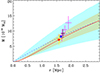 |
Fig. 6. Cluster mass profile M(r). The MAMPOSSt solution is shown with a solid red line (best fit) and orange shading (68% confidence level). The caustic solution is shown with a dashed blue line (best fit) and cyan shading (68% confidence level). The dots represent the positions of (R200, M200) in the MAMPOSSt (red) and caustic (blue) M(r). The crosses stand for other determinations of (R200, M200) with the respective one σ error bars. The black cross is our determination based on the scaling relation with the cluster velocity dispersion (the value also given in Table 1). The two yellow crosses are determinations based on the hydrostatic equilibrium of the intracluster X-ray emitting gas and the four magenta crosses are determinations based on gravitational lensing effect. The references to these values are, from left to right in the figure: Schmidt & Allen (2007), Donahue et al. (2014), Umetsu et al. (2016, 2018), Herbonnet et al. (2019), Merten et al. (2015). |
Figure 7 (middle and bottom panels) shows the mean velocity profile and the velocity dispersion profile for all member galaxies. As for the integral profiles, the first value on the left was calculated from the sample of the five galaxies closest to the cluster center, and the following values were calculated by adding the galaxies at larger radii one by one. The last values correspond to the global estimates of ⟨V⟩ and σV which were calculated for all cluster members.
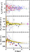 |
Fig. 7. Projected phase space and profiles of mean velocity and velocity dispersion for the member galaxies of MACS0329. Top panel: Projected phase space. The red, green, and blue symbols show red, intermediate, and blue galaxies as classified in Sect. 5 (418 galaxies; see Fig. 8). Middle panel: Mean rest-frame velocity profile for the 430 member galaxies (black full squares with error bars). Each value was computed using 30 galaxies. The small black dots show the integral profile of the mean velocity and converge by definition toward the global value ⟨Vrf⟩ = 0. The error ranges are shown by yellow lines. The magenta point indicates the rest-frame BCG velocity with its 2σ uncertainty. It is located at a large radius for easy comparison with the global value of the mean velocity. For the integral profiles calculated for blue and red galaxies, only the 1σ errors are shown (red and blue bands respectively). Bottom panel: Same as above but for the velocity dispersion profile. The integral profile for all galaxies (small black dots) converges toward the global value of σV. Red and blue open squares indicate differential profiles for red and blue galaxies. The vertical dashed lines in the three panels indicate the R200 radius. |
5. Red and blue galaxy populations
Figure 8 shows the position of the 421 cluster members with available magnitudes in the B − RC versus RC color-magnitude diagram that we used to separate red and blue galaxies. The diagram shows the presence of the two usual overdense regions, that along the red sequence and that of the blue cloud. We emphasize that our magnitudes are not k-corrected magnitudes. We verified that our subsequent classification below (based on the color B − RC) is very similar to the one we would have obtained using the color B − Z, which roughly corresponds to a rest-frame NUV-r. Wyder et al. (2007) gave the NUV-r versus r color-magnitude diagram to clearly separate galaxies into early and late populations. We prefer to use B − RC for the comparison with the other two CLASH-VLT clusters, MACS J1206.2−0847 at a similar redshift (Girardi et al. 2015) and Abell S1063 at z ∼ 0.35 (Mercurio et al. 2021), for which the color type classification shows good agreement with the respective spectroscopic type classification (see their Figs. 2 and 12). The brightest cluster galaxies are usually close to the red sequence or slightly bluer if there is relevant star formation activity. In MACS0329 the BCG is characterized by a rather blue color, (B − RC)∼(NUV − B)rf ∼ 1.4, which can be explained by a strong star formation activity probably related to the presence of a cool core (see Fogarty et al. 2015 for the UV emission and other references in Sect. 1).
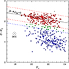 |
Fig. 8. Suprime-Cam aperture-color versus Kron-like magnitude diagram B − RC versus RC for the 421 spectroscopic cluster members with photometric information. The black solid line is the CMR, (B − RC)diff = 0. The blue dashed line shows the value (B − RC)diff = −0.5, which we used to separate green and blue galaxies (highlighted by green triangles and blue circles). The two red dashed lines show the locus of the red sequence galaxies, |(B − RC)diff|≤0.3, with the galaxies of the RedU and RedD samples marked with red circles and squares. A large black circle highlights the BCG. |
To fit the color-magnitude relation (CMR), we considered only the 269 galaxies redder than B − RC = 1.3 and applied a 2σ rejection procedure. The fitted relation is B − RC = 3.554(±0.123)−0.067(±0.006)×RC, based on 151 galaxies. The fitted CMR is similar to that obtained by Girardi et al. (2015) for the cluster MACS J1206.2−0847, as expected since the two clusters have a similar redshift (see their Fig. 2). The color (B − RC)diff is defined as the difference between the color of an observed galaxy and the corresponding CMR color at the magnitude of the galaxy.
Following Girardi et al. (2015), we classified the galaxies as follows. The Red sample consists of the galaxies with |(B − RC)diff|≤0.3 (189 galaxies), and among them, the galaxies of the RedU and RedD samples are those with positive or negative (B − RC)diff (94 and 95 galaxies, respectively). We then defined the Blue sample as the one containing 201 galaxies with (B − RC)diff ≤ −0.5. Galaxies with intermediate colors form the Green sample (28 galaxies with −0.5 < (B − RC)diff < −0.3). The BCG is not included in the Blue sample nor in the other color class samples. In total, we classified 418 galaxies, 214 of which lie within R200.
Figure 9 shows the spatial distribution of all member galaxies and in particular the fact that red galaxies are spatially more clustered than blue galaxies. To make a quantitative comparison among different galaxy populations, we applied the Kruskall-Wallis test to the cluster-centric distances R (KW test; e.g., Lederman 1984). This test is a non-parametric procedure that can be used to test whether three or more samples come from the same parent distribution. In this case, the hypothesis is rejected with a c.l. of more than 99.99%. Figure 10 shows the significant difference among the galaxies in the Red, Green and Blue samples, with the galaxies in the first groups being more clustered. We also compared the distributions of the cluster-centric distances of the RedD and RedU samples using the 1D Kolmogorov-Smirnov test (hereafter 1DKS test; Kolmogorov 1933; Smirnov 1933; see also Lederman 1984) and found no significant difference. We also found no significant difference when comparing the positions in RA and Dec of RedU and RedD galaxies according to the 2D Kolmogorov-Smirnov test (hereafter 2DKS test; Fasano & Franceschini 1987).
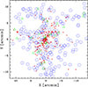 |
Fig. 9. Spatial distribution of the 430 cluster members with emphasis on the spatial segregation among galaxies of different colors. Each of the 418 classified galaxies is identified by a symbol: Red sample (small red circles), Green sample (green triangles), and Blue sample (blue circles). The large circle is centered on the BCG and encloses the R200 region. |
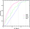 |
Fig. 10. Cumulative distributions of the cluster-centric distance R of galaxies per color-type class (see Fig. 8). Vertical dashed lines indicate the positions of one, two, and three R200. |
The application of the KW test to the rest-frame velocities Vrf – i.e., (V − ⟨V⟩)/(1 + z) – does not give a significant result, that is the velocity distributions of different color type classes can originate from the same parent distribution. This is shown in Fig. 11 where we also notice a remarkable symmetry in the distribution of galaxy velocities of all populations around the mean cluster redshift. This symmetry is quantified measuring the skewness indicator in Sect. 6. We obtained no significant differences when comparing the distributions of |Vrf|, which is consistent with the fact that there is no significant difference among the velocity dispersions of the different populations (see Table 4).
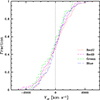 |
Fig. 11. Cumulative distributions of the rest-frame velocity Vrf of galaxies per color-type class. The dotted line corresponds to the mean cluster redshift. |
Kinematical properties of the whole cluster and galaxy populations.
Figure 7 shows the integral profiles of the mean velocity and velocity dispersion of red and blue galaxies, separately. The global mean velocities of the two populations are consistent between them and with the BCG velocity within the measurement uncertainties. The integral profile of the velocity dispersion of the blue galaxies shows a stronger decrease than that of the red galaxies. Figure 7 (bottom panel) also shows the differential profiles.
6. Substructure
Here we present our analyses and results on the features that indicate a deviation of the cluster from a dynamical equilibrium state and can be used as tracers for the cluster formation (see, e.g., Girardi & Biviano 2002 for a review). Since the sensitivity of any substructure diagnostics is known to depend on the relative position and velocity of the substructure, we performed a series of tests in velocity space (1D tests), in the space of positions projected onto the sky (2D tests), and in combined space (3D tests). Table 5 summarizes our main results on the substructure.
Results of the substructure analysis.
6.1. Analysis of the velocity distribution
The velocity distribution was analyzed for possible deviations from the Gaussian distribution, which could provide important information about the complex internal dynamics. In fact, a Gaussian distribution is assumed for the velocities of galaxies in clusters because clusters are expected to relax to an equilibrium configuration. The inspection of the phase space distribution of galaxies in Fig. 5 suggests a certain degree of persistent infall onto MACS0329 and it is known that the extent of accretion is likely related with the Gaussianity or non-Gaussianity of the velocity distribution (e.g., Sampaio et al. 2021). However, it is expected that the infall is more important for external cluster regions and blue galaxies. From this perspective, we analyzed several subsamples of the cluster data. The results of our analyses on the cluster substructure are discussed in Sect. 8.
We calculated the shape estimators proposed by Bird & Beers (1993; see their Table 2), that is the skewness (SKEW), the kurtosis (KURT), the asymmetry index (AI) and the tail index (TI). We found marginal evidence of non-Gaussianity for the whole sample (lightly tailed according to TI, in the range of 90–95% c.l.) and no evidence for the sample of galaxies within R200. Looking at the different galaxy populations, we found no evidence of substructure for the Red sample, a marginal evidence for the Green sample (platokurtic in the range of 90–95% c.l.), and a significant evidence for the Blue sample (lightly tailed according to TI and with positive AI, both in the range of 95–99% c.l.).
Based on the Indicator test of Gebhardt & Beers (1991), we also checked the peculiarity of the BCG velocity (VBCG = 135 027 km s−1) in the two samples containing the BCG (namely the TOT and R200 samples). There is no indication of an anomaly (see also Fig. 7, middle panel). To detect and analyze possible deviations from a single-peak distribution, we also applied the 1D-DEDICA method previously used in Sect. 3 to determine MACS0329 membership. For each sample, there is no evidence of a multimodal distribution.
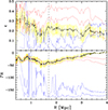 |
Fig. 12. Integral profiles of ellipticity (upper panel) and position angle (lower panel) for the entire galaxy population (solid black line and yellow errorbars) and for red and blue galaxy populations (red and blue errorbands only). The values of ϵ and PA at a given radius R have been estimated by considering all galaxies within R. The vertical dashed line shows the value of R200 (1.71 Mpc). |
6.2. Analysis of the 2D galaxy distribution
We calculated the ellipticity (ϵ = 1 − b/a, where a and b are the major and minor axes) and the position angle of the major axis (PA) of the galaxy distribution using the method of moments of inertia (Carter & Metcalfe 1980; see also Plionis & Basilakos 2002 with weight w = 1). Here PA are measured counterclockwise from north. Figure 12 shows the integral estimates of ϵ and PA at increasing radii out to 4 Mpc, where most member galaxies are contained. The results within 0.4 Mpc are too noisy to be meaningful. Table 6 lists the values of ϵ and PA for the galaxies within 4 Mpc and R200, and for the red and blue galaxies separately. The red and blue populations show a clear dicothomy. As for the blue galaxies, their distribution is consistent with a round distribution out to about to ∼3 Mpc, and only in the outermost region we detected an ellipticity ∼0.25 with a PA consistent with a north-south elongation. The distribution of the red galaxies is far from being round, reaching a value of  at R200 and similar values out to 3 Mpc. For the red galaxies, the PA is therefore already fully significant in the internal cluster region with PA =
  degrees at R200 and values between −40° and −30° in the entire investigated region, that is a SE-NW elongation. The values of ellipticity and PA of the TOT sample can be explained by the combination of the two populations, with the blue galaxies dominating in the outer cluster regions.
Ellipticity and position angle of the galaxy distribution.
We also investigated the spatial distribution of the galaxies using the 2D-DEDICA method (Pisani 1996). To better weight the substructures with respect to the cluster core, the sample of member galaxies was restricted to an RC-band magnitude of ≤24, that is a sample of 416 galaxies. This reduces the difference in spectroscopic completeness between the central region covered by the MUSE observations and other regions, since RC = 24 is approximately the limit reached by the VIMOS redshift determinations (see also Biviano et al. 2023). The only effect in the color class samples is the rejection of five blue galaxies.
Table 7 lists the full information for the relevant peaks (i.e., those with a c.l. ≥99%) with a relative density with respect to the main peak ρ ≳ 0.20 and with at least ten assigned galaxies. The relevant maps are shown in Figs. 4 and 13. As for the whole cluster, the 2D-DEDICA density reconstruction shows a main peak centered on the BCG, with two secondary, smaller peaks in the SE and NW, both within R200. The results for the R200 sample and Red sample are very similar and we do not show the corresponding figures. We also show the results for RedU and RedD samples separately, since RedU and RedD galaxies emphasize the NW peak and the SE peak, respectively (see Fig. 13, left panels). The Green and Blue samples appear to be much less concentrated than the Red sample, although both have a peak near the BCG. The spatial distribution of the blue galaxies shows no sign of SE-NW extension, but a significant southern concentration. This is consistent with the north-south extension observed in the PA analysis of the Blue sample when considering external cluster regions.
Results of the 2D-DEDICA analysis.
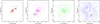 |
Fig. 13. Spatial distributions and isodensity contour maps for the four color classes: RedU, RedD, Green, and Blue samples (from left to right panels). In each panel, we show the region of interest. The large and small crosses in each box show the position of the BCG and secondary density peaks (see Table 7). The R200 region is highlighted by the circle, which is centered on the BCG. |
6.3. Combining position and velocity information
The presence of correlations between positions and velocities of cluster galaxies is always a strong indication of real substructures. To investigate the 3D cluster structure we performed two tests. The presence of a velocity gradient was searched for by performing a multiple linear regression fit to the observed velocities with respect to the galaxy positions in the plane of the sky (e.g., den Hartog & Katgert 1996; Girardi et al. 1996). Significance is based on 1000 Monte Carlo simulated clusters obtained by shuffling the velocities of the galaxies with respect to their positions. In the TOT sample we found a significant velocity gradient consistent with higher velocities in the south-southeast region than in the north-northwest region (PA =  , significant at the 94% c.l.). No significant patterns are found in other galaxy samples.
To quantify the substructure level, we used our modified version of the Δ test of Dressler & Shectman (1988), which only considers the local mean velocity indicator (hereafter DSV test; Girardi et al. 2010). This indicator is δi, V = [(Nnn + 1)1/2/σV]×(⟨V⟩loc − ⟨V⟩), where the local mean velocity ⟨V⟩loc is calculated using the i-th galaxy and its Nnn = 10 neighbors. For a cluster, the cumulative deviation is given by the value Δ, which is the sum of the |δi, V| values of the individual N galaxies. As with the velocity gradient, the significance of Δ (i.e., the presence of substructure) is based on the 1000 Monte Carlo simulated clusters.
The DSV test provides positive evidence of substructure for the entire population (99.8% c.l.). The substructure is restricted to two regions with a few low velocity galaxies, as shown in the bubble-plot of Fig. 14. The first region is located in the southwest near R200. The second region lies to the north outside R200. We also used the technique developed by Biviano et al. (2002) to compare the distribution of the δi values of the real galaxies with those of the galaxies of the simulated clusters. We compare the distributions of the δi, V values in Fig. 15. The distribution of the real galaxy values shows a tail at large negative δi, V values compared to the distribution of the simulated galaxy values. This confirms that galaxies with low velocities are probably the cause of the substructure. Comparing the two distributions with the 1DKS test, the difference is quite modest (≲90%). The DSV test finds no substructure in the R200 sample, the Red sample and the Green sample. The only exception is the Blue sample. In this case, the substructure is significant at the 99.3% c.l., and the bubble-plot again shows a region populated by low velocity galaxies in the southwest.
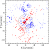 |
Fig. 14. Bubble plot of the DSV test quantifying substructures for the entire cluster population. The larger the circle, the greater the deviation of the local mean velocity from the global mean velocity. Blue and red circles indicate where the local value of the mean velocity is smaller or larger than the global value. The R200 region is highlighted by the large black dashed circle on the BCG. |
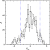 |
Fig. 15. Distribution of the δi, V values (see text and Fig. 14). The solid line histogram refers to the observed galaxies. The dashed line histogram refers to the galaxies of the simulated clusters, normalized to the number of observed galaxies. The blue vertical dashed lines mark the |δi, V|> 3 regions in which most of the real galaxies are expected to be in the 3D substructure. |
All the above analyses suggest that very few galaxies are involved in the 3D substructures. To verify this, we performed the DSV test changing the number of neighbors. The significance of the substructure decreases when using Nnn = 20 instead of Nnn = 10, to 99.4% and 93% for the TOT and Blue samples, respectively. In contrast, for Nnn = 5, the significance of the substructure increases to > 99.9% and 99.9% c.l. for the TOT and Blue samples. Figure 16 shows the bubble plot for the blue galaxies confirming the presence of a small clump of low velocity galaxies in the south-southwest.
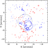 |
Fig. 16. Same as in Fig. 14 but restricted to the blue galaxies and using the DSV test with a smaller number of neighbors to detect small substructures. |
7. Exploring galaxy systems in the MACS0329 field
Here we present our analysis of the other three peaks detected in the redshift distribution, listed in Table 2. To extract the member galaxies belonging to each galaxy system (hereafter GrG1, GrG2, GrG3 in order of increasing redshift), we applied the “shifting gapper” procedure for each peak as already used in Sect. 3, with the standard parameters of Fadda et al. (1996). For each galaxy system we show the redshift distribution, the distribution in phase space and on the sky (Figs. 3, 17, and 18, respectively). For each system, details of the membership and resulting properties are given below and the global properties are summarized in Table 8.
Global properties of line-of-sight galaxy systems.
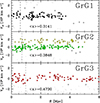 |
Fig. 17. Projected phase spaces of the three galaxy systems (GrG1, GrG2, and GrG3 in the top, middle, and bottom panels, respectively). For each system, the rest-frame velocity, Vrf, and the distance R have been computed using the group mean velocity and group center. Circles indicate galaxies that belong to the velocity peak. Full circles indicate the group members (black, green and red colors for GrG1, GrG2 and GrG3, respectively). Middle panel also shows the galaxies of a secondary peak (GrG2bis, yellow color). For each group, the vertical line shows the R200 radius and the mean redshift of the system is given (see also Table 8). |
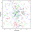 |
Fig. 18. Spatial distribution of the 89, 124, and 89 member galaxies of GrG1, GrG2, and GrG3 shown with small circles (black, green, and red as in Fig. 17). The corresponding R200 radii are represented by large black, green, and red circles. Small blue dots and the large blue circle indicate 430 members and the R200 radius of MACS0329. The black dashed circle refers to the western galaxy concentration of GrG1 (see text). Galaxies belonging to the secondary peak GrG2bis are very sparse in the field, as shown by blue crosses. The plot is centered on the BCG of MACS0329. |
As for the peak no. 1 detected in the redshift distribution, we found that the 2D spatial distribution of its galaxies shows two concentrations that are ∼5′ apart (see Fig. 18). The eastern concentration is dominated by a pair of bright galaxies surrounded by diffuse intragroup light (see Fig. 1, the GrG1 region). Unfortunately, we do not have a redshift measurement for the northeastern galaxy of the pair, but the photometric redshift is consistent with that of GrG1 (zphot = 0.321 ± 0.019 from the Dark Energy Camera Legacy Survey, DESI DR9). The southwestern galaxy is the second brightest galaxy among the galaxies in the redshift peak no. 1 (RC = 18.81, only ≲0.5 fainter than the brightest one). Therefore, we decided to assume this galaxy having spectroscopic redshift as the center of the system [RA =  , Dec = −02° 08′51.5″ (J2000.0)]. The member selection with the “shifting gapper” leads to 89 galaxies in the GrG1 structure. We calculated the mean redshift and the velocity dispersion. We used the same procedure as in Sect. 4 to obtain R200 and M200. In this way, we identified a probable group with R200 ∼ 0.6 Mpc. We note that the first brightest galaxy of the peak no. 1 is located in the western concentration, but at its edge. This is the reason why we did not analyze this concentration further. We show this western concentration in Fig. 18 (dashed circle) by using the 2D-DEDICA peak as the center and a radius with the same size as the GrG1 group.
As for peak no. 2, reapplying the 1D-DEDICA method shows the presence of two peaks (see Fig. 3, middle panel in the inset plot). The low-velocity peak is richer in galaxies and spatially quite dense around a very luminous dominant galaxy. This galaxy is projected near the center of MACS0329, ∼40″ to the northwest (see Fig. 1). Due to its relevance we obtained the spectrum at TNG (see Fig. 2); other relevant discussions can be found in Sect. 8.4. It is assumed that this galaxy is the center of the GrG2 structure [RA =  , Dec = −02° 11′29.1″ (J2000.0)]. We used the “shifting gapper” method to extract 124 members of 127 galaxies in the low velocity peak. As described above, we calculated the global properties and extracted a probable group with R200 ∼ 0.7 Mpc. The galaxies of the high-velocity peak are quite sparse in the field and we refer to this structure as GrG2bis (see blue-cross symbols in Fig. 18). They are so sparse in the field that the application of the 2D-DEDICA method splits the GrG2bis sample of 55 galaxies into 34 non-significant subsamples. The galaxies of GrG2bis could be part of a large-scale structure or, more interestingly, the remnants of a previous merger involving GrG2 and now spread across the field. In any case we no longer discuss GrG2bis.
The galaxies of the peak no. 3 show a dense concentration of galaxies centered at the southern boundary of the field sampled by our redshift catalog, ∼9′ south of MACS0329 (see Fig. 18). There is no clearly dominant galaxy and we assumed that the center is the density center estimated with the 2D-DEDICA method [RA =  , Dec = −02° 20′28.0″ (J2000.0)]. The “shifting gapper” procedure leads to 89 galaxies in the structure. As described above, we calculated the global properties and extracted a probable group with R200 ∼ 1 Mpc.
We also analyzed the region around MACS0329 using Chandra X-ray data and DESI DR9 photometric data. Figure 19, which covers an area of ∼30 × 30 arcmin in the field of MACS0329, shows the resulting galaxy systems of interest. Considering galaxies with photometric redshift close to that of MACS0329, namely those in the range 0.41 < zphot < 0.49 and with uncertainty ezphot < 0.05 (blue small symbols in Fig. 19), we applied the Voronoi Tessellation and Percolation technique (Ramella et al. 2001; see also Barrena et al. 2005; Boschin et al. 2009). The galaxies that we identified as belonging to structures with a significance at the 99.9% c.l. are marked by blue squares. We are able to recover both the SE-NW elongation of MACS0329 as well as the galaxy concentration in the southern regions, that is GrG3. This result gives us confidence that the photometric-redshifts can be used to detect galaxy systems outside the region covered by our spectroscopic catalog. We detected another system far to the south [at RA =  , Dec = −02° 26′24″ (J2000.0)] and a system to the northeast [at RA =
  , Dec = −02° 03′25″ (J2000.0)]. The latter is also detected by the Chandra X-ray data, as it is an extended emission. We identify it with the galaxy system 2CXO J033045.8−020323 listed in NED6. Instead, there is no corresponding entry in NED for the former galaxy system.
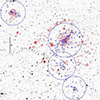 |
Fig. 19. DESI r-band image (north top and east left) of the MACS0329 with Chandra X-ray isocontour levels (in red) superimposed (energy range: 0.5−7 keV). The small blue symbols indicate galaxies whose photometric redshifts are close to that of MACS0329. In particular, the blue squares highlight galaxies belonging to significant structures according to our Voronoi analysis. Concentrations of galaxies are indicated by large blue circles. The largest circle indicates MACS0329 with its strong X-ray emission. The galaxy system to the south is already detected in the redshift space (GrG3). The system further south lies outside the region covered by our redshift catalog. The system in the northeast shows an extended X-ray emission and we identify it with 2CXO J033045.8−020323. |
8. Discussion
8.1. Global structure
Our analysis confirms that MACS0329 is a very massive cluster. Our mass estimate from the scaling relation with the velocity dispersion, M200 = (9.2 ± 1.5)×1014 M⊙ agrees with those obtained by more sophisticated techniques (MAMPOSSt and caustic methods; see Sect. 4) and fits well within the range 7 − 13 × 1014 M⊙ of values published in the literature and derived from X-ray data or gravitational lensing analyses (Schmidt & Allen 2007; Donahue et al. 2014; Umetsu et al. 2014, 2016, 2018; Merten et al. 2015; Herbonnet et al. 2019).
The SE-NW elongation of the distribution of galaxies in the plane of sky is the most important feature of the cluster structure. This SE-NW direction is essentially traced by the red galaxies and agrees with the mass distribution from the weak-lensing analysis (Donahue et al. 2016; Umetsu et al. 2018) and the ICM distribution from X-ray isophotes (Donahue et al. 2016). On smaller scales, the BCG light also follows the same SE-NW direction as shown by the HST UV and I-bands images (Donahue et al. 2015; Durret et al. 2019). The same direction is also followed by the mass distribution derived from the strong-lensing analysis (Okabe et al. 2020).
For the red galaxies within R200, we measured a position angle  degrees and the ellipticity
  . This ellipticity is higher than the ellipticity of the X-ray isophotes (ϵ ∼ 0.15; Maughan et al. 2008; Mantz et al. 2015), as it is also shown by a direct visual comparison between the galaxy distribution and X-ray emission images (cf. Figs. 1 and 4). The fact that the nearly collisionless dark matter and galaxies generally have a more elongated distribution than the ICM component is expected from simulations (McDonald et al. 2022) and confirmed by observations (Yuan et al. 2023).
The velocity dispersion profile of MACS0329 shows the typical behavior for clusters, with a modest increase in the central region and then a decrease toward external regions. For instance, Fig. 7 – bottom panel – can be compared to Fig. 2 of Girardi et al. (1998) obtained by combining 170 clusters. In the case of MACS0329, the extensive redshift catalog allowed us to obtain the individual profile and to perform a direct comparison with that of MACS J1206.2−0847, which is another CLASH-VLT cluster sampled with many redshifts (Biviano et al. 2023). Both profiles decline by a factor of ∼1.5 between 0.05 and 1 in R200 units.
8.2. Substructure from galaxies versus ICM results
Our study is the first one that uses galaxies to trace the fine structure of MACS0329. The statistical results of the substructure tests applied to the R200 sample show that MACS0329 has no significant substructure (see Table 5) with the exception of two secondary low-density peaks in the 2D galaxy distribution, which are caused by the red galaxies. Tests for substructure in velocity space or in projected phase space only lead to significant results when blue galaxies or outer cluster regions are considered. Thus, our analysis based on member galaxies supports a scenario where MACS0329 is close to a state of dynamical equilibrium.
Our results agree with Mann & Ebeling (2012) who classify MACS0329 among the relaxed cluster based on the following three criteria: a pronounced cool core, a perfect alignment of the X-ray peak, and a single BCG. We note that previous assertions of a non-relaxed status is due to the analysis of the X-ray morphology and, in particular, to a few parameters for which MACS0329 is indeed at the borderline between a status of relaxation or disturbance. According to Mantz et al. (2015), MACS0329 is classified as disturbed because it exceeds the threshold for the symmetry statistics, but this result is not so conclusive if we consider the uncertainties related to the measured value (s = 0.85 ± 0.08) compared to the threshold value of sth = 0.87. According to Maughan et al. (2008) and Sayers et al. (2013), MACS0329 is considered a disturbed cluster due to the measure of the centroid shift (w = 0.014 ± 0.003), which is not significant when compared to the threshold value wth = 0.01. More recently, Donahue et al. (2016) measure w = 0.011 ± 0.001 for MACS0329 and consider a threshold of wth = 0.02. Their Fig. 3 of X-ray concentration versus the centroid shift shows that MACS0329 resembles rather a relaxed than a disturbed cluster. Therefore, our results based on member galaxies well agree with those of Donahue et al. (2016) based on X-ray data.
We think that the only evidence for (a small scale) substructure from X-ray data comes from the study of Ueda et al. (2020) who find a spiral-like pattern in the X-ray residual image that is consistent with a gas sloshing core, a phenomenon commonly associated with a minor merger. Consistently, MACS0329 shows the presence of a radio minihalo, which is generally related to a sloshing cold front in cool cores (Giacintucci et al. 2019; Biava et al. 2024). As evidence of a past minor merger that caused the gas sloshing, we propose the two small substructures that we have detected along the SE-NW direction in the 2D galaxy distribution of all and red galaxies (see, Figs. 4 and 13).
8.3. Blue versus red galaxy populations
We have obtained detailed information on the spatial distribution of the red and blue galaxy samples. The well-known effect of morphological and color segregation in galaxy clusters (Dressler 1980; Whitmore et al. 1993) can be appreciated in Fig. 10. However, higher moments of the phase space distribution of red and blue galaxy populations can be studied here thanks to the large spatial coverage and depth of our spectroscopic sample, consisting of 189 and 201 galaxies, respectively, which are used to probe MACS0329 within a radius larger than 2 R200.
Red galaxies are characterized by a rather elongated distribution, while the distribution of the blue galaxies is globally round out to ∼3 R200 (see Fig. 12). Outside, the distribution of blue galaxies indicates the north-south direction, and indeed there is another significant southern concentration at a distance of ∼R200 (see Fig. 13 – last right panel). The DSV test for blue galaxies shows the presence of a galaxy clump in the south-southwest with a motion that has a component along the line of sight (larger blue circles in Fig. 16). This dichotomy between red and blue galaxies – that is between a more elongated distribution for red galaxies and a rounder, less concentrated but more substructured distribution for blue galaxies – is consistent with the one we found in two other clusters of the CLASH-VLT sample studied with extensive redshift catalogs: MACS J1206.2−0847 (Girardi et al. 2015) and Abell S1063 (Mercurio et al. 2021).
Our interpretation of this dichotomy is the following. Most red galaxies are likely tracing the main phase of cluster formation along a prominent SE-NW filament of the large-scale structure, likely in the plane of the sky since we detected no velocity gradient for red galaxies. It is well known that there is a strong correlation between the dynamical activity in galaxy clusters and the tendency of the galaxy distribution to be elongated and aligned with neighboring clusters (e.g., Plionis & Basilakos 2002). This is caused by the anisotropic merging along the large-scale filaments, as also shown by the analysis of simulations (e.g., Cohen et al. 2014). However, it is also known that the final distribution can be aspherical after violent relaxation (Aarseth & Binney 1978; White 1996). Therefore, the elongation of MACS0329 does not contradict the lack of statistical evidence for the presence of an important substructure. As for the blue galaxies, our results are consistent with a picture in which a cluster irregularly accretes individual spirals or clumps of mostly spiral galaxies from the field, that is blue galaxies trace the most recent infall into the cluster. In the case of MACS0329 we are able to detect two clumps of blue galaxies at a distance ∼R200. In any case, these clumps of galaxies are very loose and should be interpreted as overdensities of the large-scale structure filaments that have grown inside the cluster, and not as dense and isolated groups.
In the context of the above scenario, we also discuss the kinematical properties of the cluster galaxy populations. The global values of velocity dispersion of the red and blue galaxies agree within ∼1.3σ (see Table 4) and the agreement is also better for galaxies within R200. This result supports recent studies indicating a velocity distribution that does not depend dramatically on the color or spectral type of the galaxy population (e.g., Rines et al. 2005, 2013; Mahajan et al. 2011; Biviano et al. 2013; Girardi et al. 2015).
There is evidence that the velocity dispersion profile of blue (star forming) galaxies decreases with radius more than that of red (passive) galaxies. However, this evidence was obtained when studying galaxy samples combining many clusters (e.g., Carlberg et al. 1997; Biviano et al. 1997; Adami et al. 1998; Dressler et al. 1999). For individual clusters, the spatial morphological segregation and the sensitivity of the velocity dispersion measure make more difficult to obtain conclusive results. In the case of MACS0329 we are able to see the expected trend (see Fig. 7, bottom panel), but the significance is nonetheless small. To highlight the difference, we considered the region within 1 Mpc and obtained  km s−1 and
  km s−1 for 23 blue and 100 red galaxies, resulting in a difference of only 2.2σ. Since the cluster gravitational potential is the same for all galaxies treated as test particles, the sharper decreasing profile is interpreted as a sign of more radial orbits in external cluster regions (e.g., Biviano et al. 1997; Biviano & Katgert 2004; Mamon et al. 2019). For MACS0329, this is consistent with a scenario where blue galaxies fell into the cluster more recently.
The history of member galaxies can be traced in a more quantitative, statistical way through their position in the projected phase space (e.g., Haines et al. 2015; Deshev et al. 2020; Mercurio et al. 2021; Qu et al. 2023). We compare the distribution of galaxies in MACS0329 with the halos from the simulations of Oman et al. (2013). In Fig. 20 we show our data in a way that reproduces Fig. 4 of Oman et al. (2013), that is we plot normalized velocities Vn = |Vrf|/σV, 3D, where we have assumed  , against normalized cluster-centric distances Rn = R/Rvir (Rvir = 2 Mpc ∼1.2 R200 for MACS0329). The blue galaxies populate the region with large radii and small velocities, that is the region of the recently infalled galaxies, while the red galaxies populate the region at small radii within a triangular region bounded by the line Vn = −(4/3)Rn + 2. This line separates the regions where most galaxies have an infall time of more or less than 1 Gyr (Oman et al. 2013; see also Fig. 1 of Reeves et al. 2023). In MACS0329, within 1.5 R200, only 9% of the cluster members can be classified as recently accreted. This fraction is smaller than that in the Perseus cluster (12%; Aguerri et al. 2020) and Abell 85 (30%; Agulli et al. 2016). In agreement with our scenario for MACS0329, the fraction of recently accreted galaxies differs for blue and red galaxies (18% and 4%, respectively).
 |
Fig. 20. Projected phase space distribution of galaxies per different color type (red, green, and blue colors for Red, Green, and Blue samples) showing normalized velocities versus normalized projected cluster-centric distance. The dashed diagonal line separates the regions where most galaxies are expected to have an infall time of more or less than 1 Gyr according to the simulations by Oman et al. (2013). |
8.4. MACS0329 surroundings and line-of-sight groups
The analysis of redshift peaks is a very powerful method for detecting the presence of galaxy systems. For instance, a small peak at z ∼ 0.15, which is below the relative density threshold adopted in this study, also proved to be a real group (Girardi et al. 2023). Among the groups that we analyze in this study, GrG3 is the one closest to MACS0329 in redshift and is the only group that may have an interaction with MACS0329. It is also close in projection (less than 3 Mpc in the cluster rest frame). However, by assuming that the redshift difference is due to kinematics, one obtains that ΔVrf ∼ 4700 km s−1. This value is larger than the encounter velocity of merging clusters in cosmological simulations (e.g., Łokas 2023) and in observations (e.g., Sarazin et al. 2013; Barrena et al. 2014; Golovich et al. 2017), where 4700 km s−1 is the maximum observed value (Markevitch 2006 in the Bullet Cluster). In fact, GrG3 is gravitationally unbound to MACS0329 according to the simple Newton criterion when considering only MACS0329 as the total mass of the system. However, we could think that both MACS0329 and GrG3 are embedded in a larger structure such as a supercluster. In fact, Figs. 5 and 19 show that MACS0329 is a cluster surrounded by many galaxies in the close velocity field and by three galaxy systems with similar redshift. Unfortunately, two of these systems are out of our spectroscopic survey and we cannot perform a more precise analysis.
Finally, we emphasize that an extensive redshift survey is needed to avoid possible misunderstandings. The brightest galaxy in the GrG2 group is projected near the center of MACS0329, at ∼40″ (see Fig. 1) and was therefore wrongly interpreted as a companion galaxy of the MACS0329 BCG in the context of a post-merger scenario (DeMaio et al. 2015). Instead, the distance from GrG2 to MACS0329 in redshift is Δz = 0.0655, which, if considered of kinematical nature, corresponds to an enormous difference in velocity ΔVrf ∼ 13 500 km s−1, which rules out any interaction between MACS0329 and GrG2 and their respective brightest galaxies. Ueda et al. (2020) committed the same misunderstanding when they identified the subcluster responsible for the sloshing core with a secondary peak in the central mass distribution detected by Zitrin et al. (2015) through strong gravitational analysis (see Fig. 8 of Ueda et al. 2020). This secondary peak is located northwest of the primary X-ray peak and corresponds to the position of the brightest galaxy in the GrG2 group. In practice, the secondary peak of the mass distribution detected by Zitrin et al. (2015) is real, but it is associated with a foreground group rather than a feature of the internal structure of MACS0329.
An extensive redshift information is also necessary for a correct interpretation of results beyond studies of cluster galaxy populations. As example, we note that the visual inspection of the MACS0329 mass distribution map obtained by Umetsu et al. (2014) through the weak lensing analysis shows the presence of a second peak ∼3.5′ in the northwest (see their Fig. 1). The authors do not discuss this feature; interestingly however, this is the position of a real foreground group (GrG1, see Fig. 1). The effect of a small foreground group projected near the cluster center when deprojecting the mass distribution obtained by gravitational lensing effects is also discussed for the galaxy cluster MACS J1206.2−0847 (Biviano et al. 2023). Also in this case, the detection of the group was feasible thanks to the extensive CLASH-VLT redshift survey and led to resolve an apparent mismatch between lensing and dynamical mass profiles in the cluster core.
9. Summary and conclusions
We have presented the first analysis of the massive cluster MACS0329 based on the kinematics of the member galaxies as part of the CLASH-VLT ESO Large Program. Our analysis is based on an extensive redshift dataset of over 1700 galaxies, which probe MACS0329 within a radius of ∼3 R200. The dataset is complemented by multiband photometry based on high-quality Subaru Suprime-Cam imaging. We combined the velocities and positions of the galaxies to select 430 cluster members. Our specific results can be summarized as follows:
-
The new precise estimate of the cluster redshift is z = 0.4503 ± 0.0003. We report the first estimate of the velocity dispersion as
 km s−1. Following the recipe of Munari et al. (2013) and a recursive approach, we computed the dynamical mass as M200 = (9.2 ± 1.5)×1014 M⊙ within a radius of R200 = (1.71 ± 0.07) Mpc. Within this radius, there are 227 members for which we estimate
  km s−1.
 -
Using the B − RC versus RC diagram, we classified 418 member galaxies as blue, intermediate, or red galaxies out to ∼6 Mpc. We find strong spatial segregation among the three populations but no kinematical differences. The only exception is the stronger decrease of the velocity dispersion profile of the blue galaxies compared to that of the red galaxies, corroborating earlier findings reported in the literature for combined samples of galaxy clusters, and the difference is likely due to different orbits.
-
Most of the evidence for substructure comes from external cluster regions or the blue population. In particular, we detected two loose clumps of blue galaxies in the south and southwest at a distance of ∼R200.
-
The red galaxies show an elongated distribution with an ellipticity ϵ ∼ 0.4 tracing the SE-NW direction. This is consistent with the elongation of the ICM, which nevertheless has a lower ellipticity. However, this is expected given that the ICM is a collisional component, unlike galaxies. For the red galaxies, the only indication of substructure is the presence of two minor secondary peaks in the galaxy distribution with a relative density of ∼0.2 with respect to the main peak centered on the BCG. This elongated SE-NW main structure shows no signs of a velocity gradient, which suggests that it lies on the plane of sky.
By studying the spatial and velocity distributions of galaxies of different colors, we can sketch a probable scenario for the assembly history of MACS0329. The oldest and most important component of this massive system consists of red galaxies and traces the main phase of cluster formation along the SE-NW direction, while the blue galaxy population of MACS0329 shows a more rounded distribution and signs of substructure, consistent with a more recent and multidirectional infall of groups from the field. A comparison with the results of simulations confirmed different arrival times for red and blue galaxies. To summarize, MACS0329 is not far from dynamical equilibrium. Nevertheless, the surroundings of MACS0329 are densely populated by galaxies, and three close galaxy systems have been detected.
Our study shows that extensive redshift surveys allow galaxy systems along the line of sight to be distinguished and avoid misleading results. In the case of MACS0329, there are two foreground groups that mimic a substructure in the projected mass map obtained through gravitational lensing analyses.
Data availability
Full Table 1 is available at the CDS via anonymous ftp to cdsarc.cds.unistra.fr (130.79.128.5) or via https://cdsarc.cds.unistra.fr/viz-bin/cat/J/A+A/692/A175
We refer to RΔ as the radius of a sphere in which the average mass density is Δ times the critical density at the redshift of the galaxy system; MΔ is the mass contained in RΔ.
Website currently located at https://sites.google.com/site/vltclashpublic
Acknowledgments
We thank the referee for his/her useful and constructive comments. We acknowledge financial contributions by the grant MIUR PRIN 2017 WSCC32 “Zooming into dark matter and proto-galaxies with massive lensing clusters”. MG acknowledges financial support from the grant MIUR PRIN 2022 KCS97B: “EMC2 Euclid Mission Cluster Cosmology: unlock the full cosmological utility of the Euclid photometric cluster catalog” and financial support from the University of Trieste through the programs FRA 2023 and FRA 2024. AB acknowledges financial support from the INAF mini-grant 1.05.12.04.01 “The dynamics of clusters of galaxies from the projected phase-space distribution of cluster galaxies”. RD gratefully acknowledges support by the ANID BASAL project FB210003. This publication is based on observations collected at the European Organisation for Astronomical Research in the Southern Hemisphere under ESO programme IDs 186.A-0798 and 096.A-0105. This publication is partly based on observations made on the island of La Palma with the Italian Telescopio Nazionale Galileo (TNG), which is operated by the Fundación Galileo Galilei – INAF (Istituto Nazionale di Astrofisica) and is located in the Spanish Observatorio of the Roque de Los Muchachos of the Instituto de Astrofísica de Canarias. The DESI Legacy Imaging Surveys consist of three individual and complementary projects: the Dark Energy Camera Legacy Survey (DECaLS), the Beijing-Arizona Sky Survey (BASS), and the Mayall z-band Legacy Survey (MzLS). The complete acknowledgments can be found at https://www.legacysurvey.org/acknowledgment. The Photometric Redshifts for the Legacy Surveys (PRLS) catalog used in this paper was produced thanks to funding from the U.S. Department of Energy Office of Science, Office of High Energy Physics via grant DE-SC0007914.
References
- Aarseth, S. J., & Binney, J. 1978, MNRAS, 185, 227 [NASA ADS] [CrossRef] [Google Scholar]
- Adami, C., Biviano, A., & Mazure, A. 1998, A&A, 331, 439 [NASA ADS] [Google Scholar]
- Aguerri, J. A. L., Girardi, M., Agulli, I., et al. 2020, MNRAS, 494, 1681 [NASA ADS] [CrossRef] [Google Scholar]
- Agulli, I., Aguerri, J. A. L., Sánchez-Janssen, R., et al. 2016, MNRAS, 458, 1590 [NASA ADS] [CrossRef] [Google Scholar]
- Allen, S. W., Rapetti, D. A., Schmidt, R. W., et al. 2008, MNRAS, 383, 879 [Google Scholar]
- Ashman, K. M., Bird, C. M., & Zepf, S. E. 1994, AJ, 108, 2348 [Google Scholar]
- Balestra, I., Mercurio, A., Sartoris, B., et al. 2016, ApJS, 224, 33 [Google Scholar]
- Barrena, R., Ramella, M., Boschin, W., et al. 2005, A&A, 444, 685 [NASA ADS] [CrossRef] [EDP Sciences] [Google Scholar]
- Barrena, R., Girardi, M., Boschin, W., De Grandi, S., & Rossetti, M. 2014, MNRAS, 442, 2216 [NASA ADS] [CrossRef] [Google Scholar]
- Bartelmann, M. 1996, A&A, 313, 697 [NASA ADS] [Google Scholar]
- Beers, T. C., Flynn, K., & Gebhardt, K. 1990, AJ, 100, 32 [Google Scholar]
- Berrier, J. C., Stewart, K. R., Bullock, J. S., et al. 2009, ApJ, 690, 1292 [NASA ADS] [CrossRef] [Google Scholar]
- Bertin, E., & Arnouts, S. 1996, A&AS, 117, 393 [NASA ADS] [CrossRef] [EDP Sciences] [Google Scholar]
- Biava, N., Bonafede, A., Gastaldello, F., et al. 2024, A&A, 686, A82 [NASA ADS] [CrossRef] [EDP Sciences] [Google Scholar]
- Bird, C. M., & Beers, T. C. 1993, AJ, 105, 1596 [NASA ADS] [CrossRef] [Google Scholar]
- Biviano, A., & Katgert, P. 2004, A&A, 424, 779 [NASA ADS] [CrossRef] [EDP Sciences] [Google Scholar]
- Biviano, A., Katgert, P., Mazure, A., et al. 1997, A&A, 321, 84 [NASA ADS] [Google Scholar]
- Biviano, A., Katgert, P., Thomas, T., & Adami, C. 2002, A&A, 387, 8 [NASA ADS] [CrossRef] [EDP Sciences] [Google Scholar]
- Biviano, A., Rosati, P., Balestra, I., et al. 2013, A&A, 558, A1 [Google Scholar]
- Biviano, A., Pizzuti, L., Mercurio, A., et al. 2023, ApJ, 958, 148 [NASA ADS] [CrossRef] [Google Scholar]
- Boschin, W., Barrena, R., & Girardi, M. 2009, A&A, 495, 15 [NASA ADS] [CrossRef] [EDP Sciences] [Google Scholar]
- Caminha, G. B., Rosati, P., Grillo, C., et al. 2019, A&A, 632, A36 [NASA ADS] [CrossRef] [EDP Sciences] [Google Scholar]
- Carlberg, R. G., Yee, H. K. C., Ellingson, E., et al. 1997, ApJ, 476, L7 [NASA ADS] [CrossRef] [Google Scholar]
- Carter, D., & Metcalfe, N. 1980, MNRAS, 191, 325 [CrossRef] [Google Scholar]
- Cavagnolo, K. W., Donahue, M., Voit, G. M., & Sun, M. 2008, ApJ, 683, L107 [Google Scholar]
- Cohen, S. A., Hickox, R. C., Wegner, G. A., Einasto, M., & Vennik, J. 2014, ApJ, 783, 136 [Google Scholar]
- Czoske, O., Moore, B., Kneib, J. P., & Soucail, G. 2002, A&A, 386, 31 [NASA ADS] [CrossRef] [EDP Sciences] [Google Scholar]
- Danese, L., de Zotti, G., & di Tullio, G. 1980, A&A, 82, 322 [NASA ADS] [Google Scholar]
- DeMaio, T., Gonzalez, A. H., Zabludoff, A., Zaritsky, D., & Bradač, M. 2015, MNRAS, 448, 1162 [NASA ADS] [CrossRef] [Google Scholar]
- Demarco, R., Gobat, R., Rosati, P., et al. 2010, ApJ, 725, 1252 [NASA ADS] [CrossRef] [Google Scholar]
- den Hartog, R., & Katgert, P. 1996, MNRAS, 279, 349 [NASA ADS] [CrossRef] [Google Scholar]
- Deshev, B., Haines, C., Hwang, H. S., et al. 2020, A&A, 638, A126 [NASA ADS] [CrossRef] [EDP Sciences] [Google Scholar]
- Diaferio, A. 1999, MNRAS, 309, 610 [CrossRef] [Google Scholar]
- Diaferio, A., & Geller, M. J. 1997, ApJ, 481, 633 [NASA ADS] [CrossRef] [Google Scholar]
- Donahue, M., Voit, G. M., Mahdavi, A., et al. 2014, ApJ, 794, 136 [NASA ADS] [CrossRef] [Google Scholar]
- Donahue, M., Connor, T., Fogarty, K., et al. 2015, ApJ, 805, 177 [Google Scholar]
- Donahue, M., Ettori, S., Rasia, E., et al. 2016, ApJ, 819, 36 [Google Scholar]
- Dressler, A. 1980, ApJ, 236, 351 [Google Scholar]
- Dressler, A., & Shectman, S. A. 1988, AJ, 95, 985 [Google Scholar]
- Dressler, A., Smail, I., Poggianti, B. M., et al. 1999, ApJS, 122, 51 [NASA ADS] [CrossRef] [Google Scholar]
- Durret, F., Tarricq, Y., Márquez, I., Ashkar, H., & Adami, C. 2019, A&A, 622, A78 [NASA ADS] [CrossRef] [EDP Sciences] [Google Scholar]
- Ebeling, H., Edge, A. C., & Henry, J. P. 2001, ApJ, 553, 668 [Google Scholar]
- Fadda, D., Girardi, M., Giuricin, G., Mardirossian, F., & Mezzetti, M. 1996, ApJ, 473, 670 [NASA ADS] [CrossRef] [Google Scholar]
- Fasano, G., & Franceschini, A. 1987, MNRAS, 225, 155 [NASA ADS] [CrossRef] [Google Scholar]
- Feretti, L., Gioia, I. M., & Giovannini, G. 2002, Merging Processes in Galaxy Clusters (Dordrecht: Kluwer Academic Publishers) [CrossRef] [Google Scholar]
- Fogarty, K., Postman, M., Connor, T., Donahue, M., & Moustakas, J. 2015, ApJ, 813, 117 [Google Scholar]
- Gebhardt, K., & Beers, T. C. 1991, ApJ, 383, 72 [NASA ADS] [CrossRef] [Google Scholar]
- Geller, M. J., Diaferio, A., & Kurtz, M. J. 1999, ApJ, 517, L23 [NASA ADS] [CrossRef] [Google Scholar]
- Giacintucci, S., Markevitch, M., Venturi, T., et al. 2014, ApJ, 781, 9 [Google Scholar]
- Giacintucci, S., Markevitch, M., Cassano, R., et al. 2019, ApJ, 880, 70 [Google Scholar]
- Girardi, M., & Biviano, A. 2002, Astrophys. Space Sci. Lib., 272, 39 [NASA ADS] [Google Scholar]
- Girardi, M., Fadda, D., Giuricin, G., et al. 1996, ApJ, 457, 61 [NASA ADS] [CrossRef] [Google Scholar]
- Girardi, M., Giuricin, G., Mardirossian, F., Mezzetti, M., & Boschin, W. 1998, ApJ, 505, 74 [NASA ADS] [CrossRef] [Google Scholar]
- Girardi, M., Boschin, W., & Barrena, R. 2010, A&A, 517, A65 [NASA ADS] [CrossRef] [EDP Sciences] [Google Scholar]
- Girardi, M., Mercurio, A., Balestra, I., et al. 2015, A&A, 579, A4 [NASA ADS] [CrossRef] [EDP Sciences] [Google Scholar]
- Girardi, M., Zarattini, S., Boschin, W., et al. 2023, A&A, 671, A83 [NASA ADS] [CrossRef] [EDP Sciences] [Google Scholar]
- Golovich, N., van Weeren, R. J., Dawson, W. A., Jee, M. J., & Wittman, D. 2017, ApJ, 838, 110 [NASA ADS] [CrossRef] [Google Scholar]
- Green, T. S., Edge, A. C., Stott, J. P., et al. 2016, MNRAS, 461, 560 [Google Scholar]
- Haines, C. P., Pereira, M. J., Smith, G. P., et al. 2015, ApJ, 806, 101 [NASA ADS] [CrossRef] [Google Scholar]
- Herbonnet, R., von der Linden, A., Allen, S. W., et al. 2019, MNRAS, 490, 4889 [NASA ADS] [CrossRef] [Google Scholar]
- Inami, H., Bacon, R., Brinchmann, J., et al. 2017, A&A, 608, A2 [NASA ADS] [CrossRef] [EDP Sciences] [Google Scholar]
- Kaiser, N. 1987, MNRAS, 227, 1 [Google Scholar]
- Kolmogorov, A. 1933, G. Ist. Ital. Attuari, 4, 83 [Google Scholar]
- Kron, R. G. 1980, ApJS, 43, 305 [Google Scholar]
- Lederman, W. 1984, Handbook of Applicable Mathematics. Vol. 6,A: Statistics; Vol. 6,B: Statistics (Chichester: Wiley-Interscience Publication) [Google Scholar]
- Łokas, E. L. 2023, A&A, 673, A131 [NASA ADS] [CrossRef] [EDP Sciences] [Google Scholar]
- Mahajan, S., Mamon, G. A., & Raychaudhury, S. 2011, MNRAS, 416, 2882 [NASA ADS] [CrossRef] [Google Scholar]
- Mamon, G. A., Biviano, A., & Boué, G. 2013, MNRAS, 429, 3079 [Google Scholar]
- Mamon, G. A., Cava, A., Biviano, A., et al. 2019, A&A, 631, A131 [NASA ADS] [CrossRef] [EDP Sciences] [Google Scholar]
- Mann, A. W., & Ebeling, H. 2012, MNRAS, 420, 2120 [NASA ADS] [CrossRef] [Google Scholar]
- Mantz, A. B., Allen, S. W., Morris, R. G., et al. 2015, MNRAS, 449, 199 [CrossRef] [Google Scholar]
- Markevitch, M. 2006, ESA Spec. Publ., 604, 723 [NASA ADS] [Google Scholar]
- Maughan, B. J., Jones, C., Forman, W., & Van Speybroeck, L. 2008, ApJS, 174, 117 [NASA ADS] [CrossRef] [Google Scholar]
- McDonald, W., Obreschkow, D., & Garratt-Smithson, L. 2022, MNRAS, 516, 5289 [NASA ADS] [CrossRef] [Google Scholar]
- McGee, S. L., Balogh, M. L., Bower, R. G., Font, A. S., & McCarthy, I. G. 2009, MNRAS, 400, 937 [Google Scholar]
- Medezinski, E., Umetsu, K., Nonino, M., et al. 2013, ApJ, 777, 43 [NASA ADS] [CrossRef] [Google Scholar]
- Mercurio, A., Rosati, P., Biviano, A., et al. 2021, A&A, 656, A147 [NASA ADS] [CrossRef] [EDP Sciences] [Google Scholar]
- Merten, J., Meneghetti, M., Postman, M., et al. 2015, ApJ, 806, 4 [Google Scholar]
- Molnar, S. 2016, Front. Astron. Space Sci., 2, 7 [NASA ADS] [CrossRef] [Google Scholar]
- Munari, E., Biviano, A., Borgani, S., Murante, G., & Fabjan, D. 2013, MNRAS, 430, 2638 [Google Scholar]
- Munari, E., Biviano, A., & Mamon, G. A. 2014, A&A, 566, A68 [NASA ADS] [CrossRef] [EDP Sciences] [Google Scholar]
- Navarro, J. F., Frenk, C. S., & White, S. D. M. 1997, ApJ, 490, 493 [Google Scholar]
- Nonino, M., Dickinson, M., Rosati, P., et al. 2009, ApJS, 183, 244 [NASA ADS] [CrossRef] [Google Scholar]
- Okabe, T., Oguri, M., Peirani, S., et al. 2020, MNRAS, 496, 2591 [Google Scholar]
- Oman, K. A., Hudson, M. J., & Behroozi, P. S. 2013, MNRAS, 431, 2307 [Google Scholar]
- Owers, M. S., Nulsen, P. E. J., & Couch, W. J. 2011, ApJ, 741, 122 [Google Scholar]
- Pisani, A. 1993, MNRAS, 265, 706 [NASA ADS] [Google Scholar]
- Pisani, A. 1996, MNRAS, 278, 697 [NASA ADS] [CrossRef] [Google Scholar]
- Plionis, M., & Basilakos, S. 2002, MNRAS, 329, L47 [NASA ADS] [CrossRef] [Google Scholar]
- Poole, G. B., Fardal, M. A., Babul, A., et al. 2006, MNRAS, 373, 881 [Google Scholar]
- Postman, M., Coe, D., Benítez, N., et al. 2012, ApJS, 199, 25 [Google Scholar]
- Qu, C.-G., Yu, H., Diaferio, A., Sohn, J., & Liu, D. 2023, RAA, 23, 085007 [NASA ADS] [Google Scholar]
- Ramella, M., Boschin, W., Fadda, D., & Nonino, M. 2001, A&A, 368, 776 [NASA ADS] [CrossRef] [EDP Sciences] [Google Scholar]
- Reeves, A. M. M., Hudson, M. J., & Oman, K. A. 2023, MNRAS, 522, 1779 [NASA ADS] [CrossRef] [Google Scholar]
- Regos, E., & Geller, M. J. 1989, AJ, 98, 755 [NASA ADS] [CrossRef] [Google Scholar]
- Richard-Laferrière, A., Hlavacek-Larrondo, J., Nemmen, R. S., et al. 2020, MNRAS, 499, 2934 [Google Scholar]
- Rines, K., Geller, M. J., Kurtz, M. J., & Diaferio, A. 2003, AJ, 126, 2152 [CrossRef] [Google Scholar]
- Rines, K., Geller, M. J., Kurtz, M. J., & Diaferio, A. 2005, AJ, 130, 1482 [NASA ADS] [CrossRef] [Google Scholar]
- Rines, K., Geller, M. J., Diaferio, A., & Kurtz, M. J. 2013, ApJ, 767, 15 [NASA ADS] [CrossRef] [Google Scholar]
- Roettiger, K., Loken, C., & Burns, J. O. 1997, ApJS, 109, 307 [NASA ADS] [CrossRef] [Google Scholar]
- Rosati, P., Balestra, I., Grillo, C., et al. 2014, The Messenger, 158, 48 [NASA ADS] [Google Scholar]
- Sampaio, V. M., de Carvalho, R. R., Ferreras, I., et al. 2021, MNRAS, 503, 3065 [NASA ADS] [CrossRef] [Google Scholar]
- Sarazin, C. L., Finoguenov, A., & Wik, D. R. 2013, Astron. Nachr., 334, 346 [NASA ADS] [Google Scholar]
- Sayers, J., Czakon, N. G., Mantz, A., et al. 2013, ApJ, 768, 177 [Google Scholar]
- Schmidt, R. W., & Allen, S. W. 2007, MNRAS, 379, 209 [NASA ADS] [CrossRef] [Google Scholar]
- Scodeggio, M., Franzetti, P., Garilli, B., et al. 2005, PASP, 117, 1284 [NASA ADS] [CrossRef] [Google Scholar]
- Serra, A. L., Diaferio, A., Murante, G., & Borgani, S. 2011, MNRAS, 412, 800 [NASA ADS] [Google Scholar]
- Smirnov, N. 1933, Ann. Math. Stat., 19, 279 [Google Scholar]
- Sohn, J., Geller, M. J., Walker, S. A., et al. 2019, ApJ, 871, 129 [NASA ADS] [CrossRef] [Google Scholar]
- Springel, V., & Farrar, G. R. 2007, MNRAS, 380, 911 [NASA ADS] [CrossRef] [Google Scholar]
- Taylor, M. B. 2006, ASP Conf. Ser., 351, 666 [Google Scholar]
- Tiret, O., Combes, F., Angus, G. W., Famaey, B., & Zhao, H. S. 2007, A&A, 476, L1 [NASA ADS] [CrossRef] [EDP Sciences] [Google Scholar]
- Ueda, S., Ichinohe, Y., Molnar, S. M., Umetsu, K., & Kitayama, T. 2020, ApJ, 892, 100 [NASA ADS] [CrossRef] [Google Scholar]
- Umetsu, K., Medezinski, E., Nonino, M., et al. 2014, ApJ, 795, 163 [NASA ADS] [CrossRef] [Google Scholar]
- Umetsu, K., Zitrin, A., Gruen, D., et al. 2016, ApJ, 821, 116 [Google Scholar]
- Umetsu, K., Sereno, M., Tam, S.-I., et al. 2018, ApJ, 860, 104 [Google Scholar]
- Voges, W., Aschenbach, B., Boller, T., et al. 1999, A&A, 349, 389 [NASA ADS] [Google Scholar]
- White, S. D. M. 1996, in Gravitational Dynamics, eds. O. Lahav, E. Terlevich, & R. J. Terlevich, 121 [Google Scholar]
- Whitmore, B. C., Gilmore, D. M., & Jones, C. 1993, ApJ, 407, 489 [NASA ADS] [CrossRef] [Google Scholar]
- Wyder, T. K., Martin, D. C., Schiminovich, D., et al. 2007, ApJS, 173, 293 [Google Scholar]
- Yu, H., Tozzi, P., van Weeren, R., et al. 2018, ApJ, 853, 100 [NASA ADS] [CrossRef] [Google Scholar]
- Yuan, Z. S., & Han, J. L. 2020, MNRAS, 497, 5485 [Google Scholar]
- Yuan, Z. S., Han, J. L., Böhringer, H., Wen, Z. L., & Chon, G. 2023, MNRAS, 523, 1364 [NASA ADS] [CrossRef] [Google Scholar]
- Zitrin, A., Fabris, A., Merten, J., et al. 2015, ApJ, 801, 44 [Google Scholar]
All Tables
All Figures
|
Fig. 1. Suprime-Cam RC-band image (north top and east left) of the MACS0329 field with superimposed isocontour levels of the Chandra X-ray emission (energy range: 0.5−7 keV). Only the main cluster region is shown. Small blue circles mark cluster members (see Sect. 3). The blue label indicates the brightest cluster galaxy. Green labels and large circles indicate the two foreground groups (GrG1 at z = 0.314 and GrG2 at z = 0.385) projected onto the field of the cluster (see Sect. 7). The inset shows a color composite image of the central region (1.5 × 1.5 arcmin2) from the CLASH survey (Postman et al. 2012), which combines HST/ACS and WFC3 passbands. Member galaxies of MAC0329 and GrG2 are indicated by circles and squares, respectively (large symbols indicate the two brightest members of MACS0329 and GrG2). |
| In the text | |
|
Fig. 2. Spectrum from TNG of the brightest galaxy of the foreground GrG2 group (z = 0.385), which is projected ∼40″ to the northwest of the center of MACS0329 (see Fig. 1). The x-axis shows the rest-frame wavelength. The main spectral features are marked by their symbols. The two telluric features at ∼6900 Å and 7600 Å are also shown (marked by the earth symbol). |
| In the text | |
|
Fig. 3. Distribution of galaxy redshifts. The histogram refers to the galaxies with the spectroscopic redshift in the region of MACS0329 with 0.1 < z < 0.9. Labels indicate redshifts of the relevant peaks and the names of the corresponding galaxy systems, that is MACS0329 and other groups (see Table 2). The redshift distribution of the 533 galaxies assigned to the MACS0329 peak can be seen in the inset plot at the top left (black line histogram). The histogram with the red line refers to the 430 galaxies that are members. The BCG redshift is also shown. For each of the other groups, the respective right-hand inset panel shows the redshift distribution of the galaxies assigned to the peak and the galaxies selected as members (black and green line histograms, respectively, see Sect. 7). For GrG1 and GrG2, the arrows indicate the redshifts of the luminous galaxies that we have selected as the centers of the groups. |
| In the text | |
|
Fig. 4. Spatial distribution and isodensity contours of the cluster members with RC ≤ 24 within the 20′×20′ region centered on the BCG, corresponding to ∼7 × 7 Mpc2. Large and small crosses show the position of the BCG and the secondary density peaks (see Table 7). The R200 region is highlighted by the circle. |
| In the text | |
|
Fig. 5. Projected phase space of galaxies in the MACS0329 field with the rest-frame velocity Vrf = (V − ⟨V⟩)/(1 + z) versus the projected cluster-centric distance R. Dots show the 533 galaxies selected in the velocity peak of the cluster according to the 1D-DEDICA method. Red dots indicate the 430 galaxies that are considered true cluster members according to the second step of the member selection. The BCG position is indicated by the box at R = 0. The blue curves contain the region where Vrf is smaller than the escape velocity (see text). |
| In the text | |
|
Fig. 6. Cluster mass profile M(r). The MAMPOSSt solution is shown with a solid red line (best fit) and orange shading (68% confidence level). The caustic solution is shown with a dashed blue line (best fit) and cyan shading (68% confidence level). The dots represent the positions of (R200, M200) in the MAMPOSSt (red) and caustic (blue) M(r). The crosses stand for other determinations of (R200, M200) with the respective one σ error bars. The black cross is our determination based on the scaling relation with the cluster velocity dispersion (the value also given in Table 1). The two yellow crosses are determinations based on the hydrostatic equilibrium of the intracluster X-ray emitting gas and the four magenta crosses are determinations based on gravitational lensing effect. The references to these values are, from left to right in the figure: Schmidt & Allen (2007), Donahue et al. (2014), Umetsu et al. (2016, 2018), Herbonnet et al. (2019), Merten et al. (2015). |
| In the text | |
|
Fig. 7. Projected phase space and profiles of mean velocity and velocity dispersion for the member galaxies of MACS0329. Top panel: Projected phase space. The red, green, and blue symbols show red, intermediate, and blue galaxies as classified in Sect. 5 (418 galaxies; see Fig. 8). Middle panel: Mean rest-frame velocity profile for the 430 member galaxies (black full squares with error bars). Each value was computed using 30 galaxies. The small black dots show the integral profile of the mean velocity and converge by definition toward the global value ⟨Vrf⟩ = 0. The error ranges are shown by yellow lines. The magenta point indicates the rest-frame BCG velocity with its 2σ uncertainty. It is located at a large radius for easy comparison with the global value of the mean velocity. For the integral profiles calculated for blue and red galaxies, only the 1σ errors are shown (red and blue bands respectively). Bottom panel: Same as above but for the velocity dispersion profile. The integral profile for all galaxies (small black dots) converges toward the global value of σV. Red and blue open squares indicate differential profiles for red and blue galaxies. The vertical dashed lines in the three panels indicate the R200 radius. |
| In the text | |
|
Fig. 8. Suprime-Cam aperture-color versus Kron-like magnitude diagram B − RC versus RC for the 421 spectroscopic cluster members with photometric information. The black solid line is the CMR, (B − RC)diff = 0. The blue dashed line shows the value (B − RC)diff = −0.5, which we used to separate green and blue galaxies (highlighted by green triangles and blue circles). The two red dashed lines show the locus of the red sequence galaxies, |(B − RC)diff|≤0.3, with the galaxies of the RedU and RedD samples marked with red circles and squares. A large black circle highlights the BCG. |
| In the text | |
|
Fig. 9. Spatial distribution of the 430 cluster members with emphasis on the spatial segregation among galaxies of different colors. Each of the 418 classified galaxies is identified by a symbol: Red sample (small red circles), Green sample (green triangles), and Blue sample (blue circles). The large circle is centered on the BCG and encloses the R200 region. |
| In the text | |
|
Fig. 10. Cumulative distributions of the cluster-centric distance R of galaxies per color-type class (see Fig. 8). Vertical dashed lines indicate the positions of one, two, and three R200. |
| In the text | |
|
Fig. 11. Cumulative distributions of the rest-frame velocity Vrf of galaxies per color-type class. The dotted line corresponds to the mean cluster redshift. |
| In the text | |
|
Fig. 12. Integral profiles of ellipticity (upper panel) and position angle (lower panel) for the entire galaxy population (solid black line and yellow errorbars) and for red and blue galaxy populations (red and blue errorbands only). The values of ϵ and PA at a given radius R have been estimated by considering all galaxies within R. The vertical dashed line shows the value of R200 (1.71 Mpc). |
| In the text | |
|
Fig. 13. Spatial distributions and isodensity contour maps for the four color classes: RedU, RedD, Green, and Blue samples (from left to right panels). In each panel, we show the region of interest. The large and small crosses in each box show the position of the BCG and secondary density peaks (see Table 7). The R200 region is highlighted by the circle, which is centered on the BCG. |
| In the text | |
|
Fig. 14. Bubble plot of the DSV test quantifying substructures for the entire cluster population. The larger the circle, the greater the deviation of the local mean velocity from the global mean velocity. Blue and red circles indicate where the local value of the mean velocity is smaller or larger than the global value. The R200 region is highlighted by the large black dashed circle on the BCG. |
| In the text | |
|
Fig. 15. Distribution of the δi, V values (see text and Fig. 14). The solid line histogram refers to the observed galaxies. The dashed line histogram refers to the galaxies of the simulated clusters, normalized to the number of observed galaxies. The blue vertical dashed lines mark the |δi, V|> 3 regions in which most of the real galaxies are expected to be in the 3D substructure. |
| In the text | |
|
Fig. 16. Same as in Fig. 14 but restricted to the blue galaxies and using the DSV test with a smaller number of neighbors to detect small substructures. |
| In the text | |
|
Fig. 17. Projected phase spaces of the three galaxy systems (GrG1, GrG2, and GrG3 in the top, middle, and bottom panels, respectively). For each system, the rest-frame velocity, Vrf, and the distance R have been computed using the group mean velocity and group center. Circles indicate galaxies that belong to the velocity peak. Full circles indicate the group members (black, green and red colors for GrG1, GrG2 and GrG3, respectively). Middle panel also shows the galaxies of a secondary peak (GrG2bis, yellow color). For each group, the vertical line shows the R200 radius and the mean redshift of the system is given (see also Table 8). |
| In the text | |
|
Fig. 18. Spatial distribution of the 89, 124, and 89 member galaxies of GrG1, GrG2, and GrG3 shown with small circles (black, green, and red as in Fig. 17). The corresponding R200 radii are represented by large black, green, and red circles. Small blue dots and the large blue circle indicate 430 members and the R200 radius of MACS0329. The black dashed circle refers to the western galaxy concentration of GrG1 (see text). Galaxies belonging to the secondary peak GrG2bis are very sparse in the field, as shown by blue crosses. The plot is centered on the BCG of MACS0329. |
| In the text | |
|
Fig. 19. DESI r-band image (north top and east left) of the MACS0329 with Chandra X-ray isocontour levels (in red) superimposed (energy range: 0.5−7 keV). The small blue symbols indicate galaxies whose photometric redshifts are close to that of MACS0329. In particular, the blue squares highlight galaxies belonging to significant structures according to our Voronoi analysis. Concentrations of galaxies are indicated by large blue circles. The largest circle indicates MACS0329 with its strong X-ray emission. The galaxy system to the south is already detected in the redshift space (GrG3). The system further south lies outside the region covered by our redshift catalog. The system in the northeast shows an extended X-ray emission and we identify it with 2CXO J033045.8−020323. |
| In the text | |
|
Fig. 20. Projected phase space distribution of galaxies per different color type (red, green, and blue colors for Red, Green, and Blue samples) showing normalized velocities versus normalized projected cluster-centric distance. The dashed diagonal line separates the regions where most galaxies are expected to have an infall time of more or less than 1 Gyr according to the simulations by Oman et al. (2013). |
| In the text | |
Current usage metrics show cumulative count of Article Views (full-text article views including HTML views, PDF and ePub downloads, according to the available data) and Abstracts Views on Vision4Press platform.
Data correspond to usage on the plateform after 2015. The current usage metrics is available 48-96 hours after online publication and is updated daily on week days.
Initial download of the metrics may take a while.