| Issue |
A&A
Volume 692, December 2024
|
|
|---|---|---|
| Article Number | A61 | |
| Number of page(s) | 12 | |
| Section | Numerical methods and codes | |
| DOI | https://doi.org/10.1051/0004-6361/202449921 | |
| Published online | 03 December 2024 | |
Multi-step reconstruction of radio-interferometric images
Université Côte d’Azur, Observatoire de la Côte d’Azur, CNRS,
06000
Nice,
France
★ Corresponding author; This email address is being protected from spambots. You need JavaScript enabled to view it.
Received:
10
March
2024
Accepted:
9
October
2024
Abstract
Context. The large aperture arrays for the currently under construction SKA Observatory (SKAO) will allow for observations of the universe in the radio spectrum at unprecedented resolution and sensitivity. However, these telescopes will produce data on the scale of exabytes, introducing a slew of hardware and software design challenges.
Aims. This paper proposes a multi-step image reconstruction framework that allows for partitioning of visibility data by baseline length. This enables more flexible data distribution and parallelization, aiding in processing radio-astronomical observations within given constraints. Additionally, as each step of the framework only relies on a subset of the total visibilities, one can perform reconstruction progressively, with the initial step performed on the SKAO Science Data Processors and the second on local clusters.
Methods. The multi-step reconstruction is separated into two steps. First a low-resolution image is reconstructed with only short-baseline visibilities, and then using this image together with the long-baseline visibilities, the full-resolution image is reconstructed. The proposed method only operates in the minor cycle, and it can be easily integrated into existing imaging pipelines.
Results. We show that our proposed method allows for partitioning of visibilities by baseline without introducing significant additional drawbacks, reconstructing images of similar quality within similar numbers of major cycles compared to a single-step all-baselines approach that uses the same reconstruction method as well as compared to multi-scale CLEAN.
Key words: methods: data analysis / methods: numerical / techniques: image processing / techniques: interferometric
© The Authors 2024
 Open Access article, published by EDP Sciences, under the terms of the Creative Commons Attribution License (https://creativecommons.org/licenses/by/4.0), which permits unrestricted use, distribution, and reproduction in any medium, provided the original work is properly cited.
This article is published in open access under the Subscribe to Open model. This email address is being protected from spambots. You need JavaScript enabled to view it. to support open access publication.
1 Introduction
Radio-interferometry allows one to obtain images of the sky in the radio spectrum by using antenna arrays in tandem with aperture synthesis. The upcoming SKA Observatory (SKAO)1 will be composed of two separate telescopes, one for high frequencies (350 MHz–15.35 GHz) and one for low frequencies (50–350 MHz), that are currently being built separately in South Africa and Australia. Upon completion, they will provide unprecedented resolution and sensitivity, enabled by the 197 dishes in SKA-Mid in South Africa and the 512 antenna stations in SKA-Low in Australia.
With the large number of antennas comes an equally large amount of data. For SKA-Mid, projections estimate up to 2.375 TB/s = 205.2 PB/day from the dishes to the beamformer and correlator engines and 1.125 TB/s = 97.2 TB/day from these to the imaging super computer, the SKA-Mid Science Data Processor (Swart et al. 2022). For SKA-Low, the estimated data transfer is 0.725 TB/s ≈ 62.5 PB/day from the antennas to the correlator and 0.29 TB/s ≈ 25 PB/day from the correlator to the SKA-Low Science Data Processor (Labate et al. 2022). Such amounts of data naturally lead to hardware and software design challenges. These include transferring data between nodes, which turns out to be very expensive both in terms of computational time and energy, and long-term data storage, which proves impossible given the cost. In addition, memory usage per Science Data Processor node is a potential concern.
With these complications comes the need to efficiently partition both the data and the workload. This is typically performed along the frequency and time domains, with reconstruction being performed independently for each partition. Approaches that separate the image into facets for direction-dependent calibration, such as Cornwell & Perley (1992); Van Weeren et al. (2016); Tasse et al. (2018), also enable partitioning by the spatial image domain. In addition to the above, one can also potentially separate the sample data (i.e., visibilities based on the length of their corresponding baselines). However, this is typically not done due to current minor-cycle reconstruction algorithms needing to process all baselines together to achieve full resolution. This limits parallelization flexibility. For example (de)gridding needs to wait for the reconstruction algorithm to finish processing all baselines before restarting, and memory access patterns become complex for large numbers of baselines due to the large number of visibilities needing to be gridded to the same grid.
This paper proposes an image reconstruction framework that allows for the partitioning of visibilities by baseline length. It achieves this by performing reconstruction in two steps, with each processing only a subset of the total visibilities. The first produces a low-resolution image using only the short baseline visibilities. The second produces the final reconstructed image using both the long baseline visibilities as well as the low- resolution image of the first step. This approach is advantageous over previous ones, as there is no need to gather the gridded visibilities each major cycle in order to perform (de)gridding, with the only communication between nodes being an image transfer between the two steps. This also allows for the possibility of progressive reconstruction in cases where the SKA Science Data Processors are not able to fully process the visibilities within the given time constraints and the work has to be offloaded to regional clusters.
We study the proposed framework in the context of a reconstruction method in the family of algorithms that are based on compressive sensing and convex optimization (Wiaux et al. 2009; Carrillo et al. 2014; Garsden et al. 2015) adapted to the traditional major-minor cycle pipeline. We compare our framework to both a single-step approach that processes all baselines simultaneously using the same reconstruction method as well as multi-scale CLEAN (Cornwell 2008). We found it to reconstruct images of comparable quality in similar numbers of major cycles compared to the other two methods.
The remainder of this paper is structured as follows: We provide a brief overview of radio-interferometric imaging as well as a literature review in Sect. 2. We describe our method in Sect. 3, and Sect. 4 describes the datasets used for our experiments. We present and discuss our results in Sect. 5, and we provide conclusions and discuss possible avenues for future work in Sect. 6.
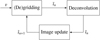 |
Fig. 1 High-level overview of the radio-interferometric pipeline. A reconstructed image în is compared to the measurements v in the (de)gridding step, which outputs the difference in the spatial domain ĩn. This is passed to the reconstruction algorithm, which generates the next estimate în+1 by deconvolving the residual image ĩn and adding it to în. |
2 Radio-interferometric imaging
Radio-interferometers measure the sky using arrays of antennas (i.e., aperture arrays). Baselines produce visibilities, which are the correlated instrumental response of the electrical field for some given time duration and electro-magnetic frequency. These can be defined using the following equation (Smirnov 2011):
 (1)
(1)
where C represents the direction-independent effects, such as antenna gain; D denotes the direction-dependent effects, such as phase gradients caused by the Earth’s ionosphere; (u, v, w) is the difference between antenna coordinates in the frame, where w is aligned with the phase center; (l, m) are the spatial angular coordinates on the celestial sphere, which is also the domain of the integral; and I is the incident radiance of the sky emission.
If the D and e−2πiw(n−1) terms are ignored, Equation (1) simplifies into a two-dimensional Fourier transform and allows one to retrieve an image of the sky emission through its inversion. This image contains artifacts caused both by the partial sampling of the Fourier domain due to the geometry of antenna arrays and by the omission of the w and D terms. Radio-interferometric imaging aims to correct for these, reconstructing an image that is usable for science.
The general approach used by radio-interferometric algorithms is iterative and is illustrated in Fig. 1. The current image estimate, în, is evaluated against the measurements, v, in the (de)gridding step, which also corrects for the w and sometimes the D terms. This step produces the difference between v and în in the image space, termed ĩn. It can be expressed as
 (2)
(2)
where F and F† respectively are the fast Fourier transform (FFT) and its inverse, G is a degridding operator responsible for extrapolating the regular gridded visibilities to their original irregular positions, and G† is the gridding operator responsible for interpolating the irregular visibilities to regular gridded positions.
The correction of the w and D terms typically occurs before F†. There are various approaches to this, such as treating the w and D terms as convolution kernels in the Fourier domain and convolving them with the visibilities during G† (Cornwell et al. 2008; Bhatnagar et al. 2008; Van Der Tol et al. 2018); discretizing in the w-plane, which can be seen in methods such as w-stacking (Offringa et al. 2014) and its improvement (Ye et al. 2022); discretizing in the time domain, such as with the snapshots method (Ord et al. 2010); discretizing in the spatial domain with facet-based approaches (Cornwell & Perley 1992; Tasse et al. 2018); or some hybrid of the above, such as between w- projection and snapshots (Cornwell et al. 2012) and w-projection and w-stacking (Pratley et al. 2019a).
The residual image ĩn is then sent to the deconvolution algorithm, which removes the partial sampling artifacts. There are a plethora of methods that aim to achieve this, with some examples being CLEAN and its variants (Högbom 1974; Cornwell 2008; Rau & Cornwell 2011) that deconvolve ĩn in a greedy non-linear manner, much akin to matching pursuit (Mallat & Z. 1993) and convex optimization methods based on compressive sensing (Wiaux et al. 2009; Carrillo et al. 2014; Dabbech et al. 2015). There has also been work done on progressively reconstructing the final image based on subsets of visibilities, such as the work of Cai et al. (2019), which shares similar general ideas to our approach. It differs in that the partitioning is by time rather than baseline, with their method still requiring all baselines to be present within a subset of visibilities. Another method that has similarities with ours is that of Lauga et al. (2024), where they alternate reconstruction between low and full-resolution iterations. Their work differs from ours in that their framework is primarily aimed at accelerating reconstruction, and it does not allow for easy partitioning of visibilities.
After deconvolution, the image estimate is updated by adding to it the deconvolved residual īn :
 (3)
(3)
The deconvolution step is iterative, ergo the imaging pipeline has a nested loop structure, which is often referred to as the majorminor loop structure, with the loop shown in Fig. 1 being the major loop and the deconvolution being the minor.
(De)gridding is often the bottleneck of the imaging pipeline due to the sheer number of visibilities needed to be processed, with the work of Tasse et al. (2018) demonstrating that it can reach up to 94% of the total processing time for a fully serial implementation. Due to this fact, there is much work that looks to expedite this stage through parallelization.
This can be done in a coarse- or fine-grained manner. Finegrained approaches aim to parallelize on the local machine at a fine scale, such as per visibility or grid cell. There has been substantial amounts of work done in this area, both for the central processing unit (CPU), such as in Barnett et al. (2019), as well as the graphics processing unit (GPU), such as in Romein (2012); Merry (2016); Veenboer et al. (2017). Our method does not deal with parallelization on this scale and instead focuses primarily on facilitating distribution and parallelization on coarser scales.
Coarse scale parallelization looks to distribute (de)gridding across multiple nodes within a cluster. A typical method for this is to distribute according to frequency channels and time. More recently, there has also been work that looks to distribute the gridding according to facets (Monnier et al. 2022) as well as sections of the UV plane (Onose et al. 2016; Pratley et al. 2019b). These different distribution strategies can also be combined, such as in the work of Gheller et al. (2023) where visibilities are separated by time and the v-axis.
Of the aforementioned coarse-scale methods, the most similar to our work are those by Onose et al. (2016) and Pratley et al. (2019b), both of which distribute and parallelize by regions of the UV grid, or also by baseline length in the case of Pratley et al. (2019b). Although similar in goal, their work differs from ours in that our presented method is not parallel, with our main focus being on investigating partitioning visibilities in the context of radio-interferometric imaging. Furthermore, although our framework is theoretically general, we present it in the context of a major-minor loop reconstruction method, solving for a deconvolution every major loop. This is contrary to both of these works, which aim to directly solve for the measurement equation using primal-dual methods. This has efficiency implications, as while their methods need to perform (de)gridding at every iteration of the optimization algorithm, our approach only needs to do so for each major cycle, which occurs far less often.
3 Proposed algorithm
Our proposed framework performs imaging in two steps, each operating only on a subset of the visibility data separated in the UV plane. These subsets, termed Vℒ and Vℋ , are partitioned according to the domains ℒ and ℋ , which cover regions representing short and long baselines, respectively.
Each step performs the entire imaging pipeline and produces an image. The first produces a low-frequency image, îℒ, from Vℒ , and the second produces the fully reconstructed image, î, using both Vℋ and îℒ.
The reconstruction method we apply to our framework is based on convex optimization with sparsity regularization, as this has a solid theoretical foundation (Candes et al. 2006; Donoho 2006; Candès et al. 2011) and has been extensively studied in the field of radio-interferometric imaging (Wiaux et al. 2009; Carrillo et al. 2014; Dabbech et al. 2015). Specifically, similar to previous works on reconstruction within the Low- Frequency Array (LOFAR) pipeline (Jiang et al. 2015; Garsden et al. 2015), we solve for a sparse series of atoms α of a redundant wavelet dictionary W.
We adapted the method to operate with the traditional majorminor loop framework for efficiency, which we achieved by making the same assumption as algorithms such as CLEAN, namely that F†G†GFi ≈ Hi, where H denotes the convolution by the point spread function (PSF). This allows the minor cycles to only solve the deconvolution problem, with the full measurement operator (i.e., degridding and gridding) only needing to be performed every major cycle. As with CLEAN, this assumes that the errors introduced by the approximation will be detected and corrected for in future major-cycle iterations. It is important to note that although detailed for this specific family of reconstruction algorithms, our proposed framework can be adapted to other reconstruction frameworks.
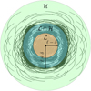 |
Fig. 2 Full set of visibilities partitioned according to the domains. The domain ℒ (orange) contains the short baseline visibilities, and ℋ (green) contains the long baseline visibilities. These are not mutually exclusive but rather have an overlap region indicated in cyan and defined using ℓ, which is the middle of ℒ ∩ ℋ, and δ, the half-width of ℒ ∩ ℋ. |
3.1 Partitioning visibilities
We partitioned the visibilities into subsets Vℒ and Vℋ based on whether the visibilities fall under the domain ℒ or ℋ , respectively. Figure 2 illustrates this, where visibilities in the orange region are part of Vℒ, and visibilities in the green belong to Vℋ. It can be seen that  , and this overlap is denoted by the cyan region. This is to alleviate cases where gridding introduces additional spatial frequencies not in the respective domain, which is caused by the visibilities being interpolated onto the grid through convolution using a kernel with a non-zero support size. The visibilities in ℒ ∩ ℋ are weighted so that although duplicated, their contribution adds up to one. This was done using filters that are discussed in Sect. 3.3.
The dataset was partitioned using the variables ℓ and δ, where δ defines the half-width size of ℒ ∩ ℋ and ℓ defines the center of ℒ ∩ ℋ. These are also shown in Fig. 2. These values are typically defined in units wavelength. However, we opted to use pixel distances in our paper.
3.2 Low-resolution reconstruction
The first step of the framework involves reconstructing a low- resolution image from Vℒ. To do this, for every major-cycle iteration, n, for a total of N cycles, we solve for the unconstrained problem:
 (4)
(4)
where  is the current residual image (i.e., between Vℒ and
  , computed in the nth major cycle), Hℒ is the operator detailing the convolution by the PSF associated with Vℒ,
  is the regularization parameter associated with the current major cycle, and
  is the deconvolved residual of
  . The final image after N major cycles is then
  .
.
An undesirable side effect when solving for Equation (4) is that îℒ can contain frequency information that is not associated with ℒ due to W not being constrained to ℒ, which interferes with the reconstruction of the full-resolution image. We handled this in the full-resolution reconstruction step using filtering, which we discuss in Sect. 3.3.
3.3 Full-resolution reconstruction
The second step of the framework reconstructs the full-resolution image using both Vℋ and îℒ. We formulated the reconstruction problem using two data fidelity terms one for the high frequencies and one for the low frequencies, in addition to an L1 regularization term. For every major-cycle iteration, n, over N total cycles, we solve for
 (5)
(5)
where  is the current residual image between Vℋ and în−1, Hℋ the operator detailing convolution by the PSF associated to Vℋ, and
  is the regularization parameter for the nth major cycle of the full-resolution step. Operator Gℒ denotes a low-pass linear filter that discards frequencies not in ℒ, and Gℋ is a high- pass linear filter that discards frequencies not in ℋ. Finally, īn is the deconvolved residual image using both
  and îℒ. The final reconstructed image is computed similarly to the low-resolution step and is
  .
.
In Equation (5), the first data fidelity term aims to reconstruct the high-frequency components of the residual image from Vℋ (i.e.,  for the nth major loop). The second data fidelity term guarantees that the low-frequency components of the reconstructed image match the reconstruction obtained using Vℒ in the first low-resolution reconstruction step. For the nth major loop, the low-pass filtered reconstructed image must match the residual between îℒ and the low-frequency components of the reconstructions at the previous major loop iterations:
  . As mentioned in the previous section, îℒ may contain spatial frequencies not in ℒ due to W not being limited to ℒ, which may bias the reconstruction of î toward these frequencies. These components are removed by applying Gℒ also to îℒ, as in Equation (5).
The gains of the two filters have to be properly normalized, in particular in ℒ ∩ ℋ , to account for visibilities being duplicated. We assumed that the two filters Gℒ and Gℋ have circularly symmetric frequency responses denoted as ɡℒ(r) and ɡℋ(r). We considered that  contains some reconstruction noise with variance η2 and that
  has noise with variance σ2. This suggests defining the two filters as
 (6)
(6)
 (7)
(7)
 (8)
(8)
These constraints ensure normalization of the variance noise across the three frequency domains ℒ − ℋ , ℋ − ℒ, and ℋ ∩ ℒ
We propose defining the frequency response of the filters for ℓ − δ < r < ℓ + δ as
 (9)
(9)
 (10)
(10)
where α(r) is such that η2ɡℒ(r)2 + σ2ɡℋ(r)2 = 1. An example is given in Fig. 3.
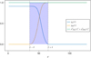 |
Fig. 3 Radial frequency response of Gℋ and Gℒ for σ2 = 1 and η2 = 1.2. |
3.4 Optimization algorithm
We opted to use the fast iterative shrinkage-thresholding algorithm (FISTA) (Beck & Teboulle 2009) for our optimization algorithm. FISTA is a fast converging algorithm aimed at optimizing convex problems that comprise both a smooth term and a term that has an easy to solve proximal operator. Equations (4) and (5) both fall under this umbrella.
1: Initialize βp, α ← βp
2: for k = 1… N − 1 do
3: β ← τγ(α − µ∇f(α))
4: 
5: βp ← β
6: end for
7: return α
FISTA operates iteratively and involves computing the gradient of the smooth portion and the proximal operator of the nonsmooth portion, which for the L1-norm is the soft-thresholding operator. It then computes the candidate solution for the next iteration using a gradient step size, µ; a soft-thresholding step size; and a momentum term to allow for faster convergence. We describe FISTA in Algorithm 1.
FISTA requires the gradients of the objective function for each iteration. These are, for the nth major cycle,
 (11)
(11)
 (12)
(12)
for Equations (4) and (5) respectively. The gradient step size is set as  , where ϑ is the Lipschitz constant of ∇f (α), defined for our problem as
 (13)
(13)
 (14)
(14)
for Equations (4) and (5) respectively, where λmax is the largest eigenvalue.
In the case where W consists of the concatenation of M orthogonal decompositions, as in Onose et al. (2016), and the convolutions are circular, we obtain the following:
 (15)
(15)
 (16)
(16)
where  denotes the discrete Fourier transform of the PSF associated to A. In other cases, such as in Starck et al. (2007), λmax can be obtained using an algorithm such as power iteration.
Finally, there is the question of how to approximate σ2 and η2 and how to select the regularization parameters λℒ and λℋ. The former is discussed in Sect. 4.3, whereas the latter is presented in Appendix A.2.
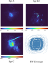 |
Fig. 4 Ground truth images of our three datasets obtained by cutting out and tapering sections of the 1.28 GHz Meerkat galactic center mosaic (Heywood et al. 2022). The images are 512 × 512 pixels in size with a resolution of 1.1″ per pixel. The UV coverage for our simulated datasets is shown at the bottom right. The same coverage was used for all three datasets. |
3.5 Implementation
We implemented our method in Julia (Bezanson et al. 2017) and integrated it into the Radio Astronomy Simulation, Calibration and Imaging Library (RASCIL) (Cornwell et al. 2020) framework under the clean algorithm name mstep. Our implementation and results as well as instructions on how to use our code are available in our repository2, with code specific to this paper available as a release3 .
4 Simulated datasets
4.1 Full datasets
We used three different simulated datasets for our experiments. They were obtained from 512 × 512 pixel tapered cutouts of the 1.28 GHz MeerKAT mosaic (Heywood et al. 2022) and consist of the regions surrounding Sgr A, B2, and C with pixel resolutions of 1.1″. These can be seen along with their UV coverage in Fig. 4.
We used RASCIL to generate the visibilities. We first generated the visibility positions using a telescope configuration detailing the 64 MeerKAT dishes, assuming that the observation lasts 4 hours (−2 to 2 hour angles) and with visibilities sampled every 120 s, resulting in 249 600 unique positions. We then performed an FFT on our ground-truth images to obtain their respective gridded visibilities, which we degridded to the generated irregular positions with uniform weighting using the improved w-stacking gridder (Ye et al. 2022). Finally, we modeled the noise received by antennas by perturbing the visibilities with noise sampled from 𝒩(0, σ/50), where σ is the standard deviation of the visibilities. A more thorough study of how noise affects our reconstruction method is outside the scope of this paper.
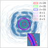 |
Fig. 5 Visualization of partition configuration parameters δ and ℓ used for our datasets. We only show δ for ℓ = 55 in this figure to avoid clutter. The combinations of the three values of δ and three values of ℓ result in nine different partitioning configurations per dataset. |
4.2 Partitioning configurations
We partitioned each initial dataset with three different centers of separation, ℓ, and each had three different half-width sizes, δ, resulting in nine different partitioning configurations for each. Figure 5 illustrates both ℓ and δ in the context of our datasets, whereas Table 1 details the number of visibilities in Vℒ and Vℋ for each configuration. It also details the number of duplicated visibilities, which lie in the region ℒ ∩ ℋ. These numbers are identical for all three of our datasets, as they have the same observational parameters. We show an example of how the partition configuration affects the dirty images for the Sgr A dataset in Fig. 6.
4.3 Visibility and reconstruction variance
Our proposed method requires knowing the variances σ2 and η2 of ĩℋ and îℒ respectively. Ensemble statistics are required to estimate them, and thus these statistics need to be approximated. To derive an appropriate strategy, we first computed estimations using ensemble populations of 50 for both Vℒ and Vℋ , each with independently sampled and identical noise properties to the original.
For σ2 , we used the average per-pixel variances of the different realizations of  computed from the different realizations of Vℋ using RASCIL. For η2, we reconstructed îℒ over three major cycles for each realization of Vℒ, and then we set η2 to be equal to the average of the per-pixel variance among these reconstructions. For the reconstructions, we used the regularization parameter
  for the nth major cycle as well as the concatenation of the first eight Daubechies wavelets for our dictionary. These choices are discussed in Appendix A.
We approximated σ2 with  by first estimating the variance of pixels in
  within a 5 × 5 sliding window and then averaging the values. Approximating η2 is more complicated, as it is dependent on the details of the reconstruction algorithm in the low-resolution step. For example, an exceedingly large value of λℒ would result in η2 = 0, as all realizations of îℒ will be zero. Rather than deriving a strategy for this, we applied a constant factor of
  for our experiments, as we observed this to be roughly the relationship between the two variables for many cases.
Table 2 shows η2 and σ2 for the different values of ℓ as well as our estimated values  . We set δ = 5 and did not vary it, as it does not significantly change the variance. It can be seen that
  is relatively close to σ2, diverging by at most 2.75×, and in most cases it is much closer to the estimated value. Although our approximations for η2 are also close in some cases, there are others where they are off by more than a factor of ten, with the worst being for the dataset Sgr B2 with ℓ = 35, where
  is almost 100 times larger. In practice, we found that these variations did not greatly change the quality of the final reconstruction. However, investigation into better approximation strategies may yield improved convergence speeds.
Visibilities per partition.
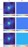 |
Fig. 6 Dirty images |


Estimated σ2 and η2 and their approximations.
5 Simulation results
We evaluated our proposed multi-step method by first studying how the partitioning configuration affects the final image reconstruction, both in terms of quality and speed. We then compared our method against a method that reconstructs with all baselines in ℒ ∪ ℋ in a single step, which afforded us information on how partitioning visibilities by baseline compares to processing all the visibilities simultaneously without any partitioning. We also performed a comparison to images reconstructed using RASCIL’s multi-scale CLEAN implementation in order to evaluate how our method compares to current popular methods used in production.
For our algorithm parameters, we set λn,  , and
, and  for the nth major cycle to
  , and
, and  , respectively, and for W, we used a concatenation of the first eight Daubechies wavelets. We discuss our motivations for these in Appendix A. We used a static value of 100 FISTA iterations as the stopping condition for both the single-step full-resolution method as well as for both steps in our multi-step method.
For multi-scale CLEAN, we used a maximum of 2000 minor iterations per major cycle, with a clean threshold of 0.001, a clean fractional threshold of 0.01, and CLEAN scales of [0, 1, 2, 4, 6, 10, 30]. Although these parameters are conservative, we found that they are necessary in reconstructing many of the smaller scale features, with larger CLEAN scales or higher thresholds leading to significantly poorer quality images.
Finally, we evaluated our reconstructions using peak signal-to-noise ratio (peak S/N), which we calculated as  to obtain the decibel (dB) value, where i is the ground truth and î is the reconstruction without the final added residual. We opted to use this rather than the maximum signal, as it evaluates the reconstruction over the entire image while maintaining a greater importance for brighter sources.
Final reconstruction quality across partition configurations.
5.1 Partition configuration effect on reconstruction accuracy
Table 3 compares the peak S/Ns in dB of the final reconstructed images for each partition configuration. These reconstructions were obtained by running the multi-step reconstruction algorithm for five low-resolution and five full-resolution major cycles.
We found that there are only slight differences between the peak S/Ns when varying ℓ, without any obvious trend. This led us to believe that the difference in final image quality is caused mainly by the choice and approximation of λ, σ2 , and η2. This is advantageous, as it implies that one can adjust the partition sizes to suit ones needs without drastically impacting the quality of the final reconstructed image. We also found that the choice of δ does not greatly impact the quality of the final image. This could be because it only affects a few spatial frequencies, and thus the effect on the final image quality is dominated by other factors, such as parameter selection. Practically, it means that one can decrease δ without greatly impacting the final reconstructed image, reducing the number of duplicate visibilities. However, care needs to be taken, as reducing δ too much may result in frequency spillage, biasing the reconstruction.
5.2 Reconstruction speed
We evaluated two aspects of reconstruction speed: the number of major cycles required for convergence, and the number of required FISTA iterations. We evaluated the latter solely in the context of the first major cycle, as this is where the majority of information is reconstructed.
Figure 7 shows the progression of the peak S/Ns of the reconstructed images across major cycles. We normalized these by the maximum obtained peak S/N for the configuration across the major cycles for easier comparison. We found that for the low-resolution step, a lower value of ℓ often results in a minor increase in convergence speed. This is expected, as a lower ℓ corresponds to a simpler image to reconstruct. However, this is counteracted in the second step, where the corresponding configurations have more information and are more challenging to reconstruct. This can also be seen for the Sgr B2 and Sgr C datasets, which have more information in  and thus have a worse initial reconstruction quality than the Sgr A dataset.
A surprising result is that the full-resolution step converges after at most only two major cycles. There are two main reasons for this. The first is due to us selecting a larger λ to maximize peak S/N, which leads to deconvolved images in the later major cycles being zero, as the regularization term dominates the data fidelity term. We experimented with regularizing less aggressively, but we found that the deconvolved images, despite still reducing the residual, overfits the noise, detracting from the overall peak S/N. We supply some results in Appendix A.2 to illustrate this outcome. The second reason is that the peak S/N is dominated by large-scale features that have already been reconstructed in the low-resolution step.
Figure 8 shows the peak S/N of the candidate solutions across FISTA iterations for both reconstruction steps and their respective first major-cycle iterations. We set îℒ to be a low-pass filtered version of the ground truth for the full-resolution step for these reconstructions. We observed a slight change in the low-resolution step reconstruction speed when varying ℓ, but we observed a much more significant change in the full-resolution step. This is expected, as the low-resolution reconstruction is simpler than the full one and uses less FISTA iterations, so changes are less pronounced. We note that for the low-resolution step, although lower values of ℓ typically result in faster initial improvement, they do not guarantee that the final image will be of higher quality, such as with the Sgr B2 dataset. However, there are additional influencing factors in these cases, such as differences in ideal parameters. Thus, whether the final difference in image quality is due to ℓ specifically is inconclusive. It should be noted that despite this, the different configurations all converge to roughly similar peak S/N values, as shown in Sect. 5.1.
Taking into account the reconstruction speeds for both majorcycle and FISTA iterations, the slight change in FISTA iterations is counteracted by the larger number of required major cycles for the low-resolution step, and vice versa for the full-resolution step. Thus, we can conclude that the choice of ℓ and δ should not greatly change the reconstruction speed, as the gains and losses roughly cancel out.
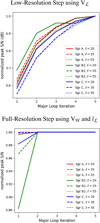 |
Fig. 7 Progression of peak S/N of reconstructed images for various partitioning configurations across the major cycles for both the low- and full-resolution reconstruction steps. peak S/Ns have been normalized by the maximum value of each configuration to allow for easier comparison. An exponential scale is used for the bottom image to better illustrate the differences between the different configurations. We fixed δ = 5 here, as we found it does not greatly impact the results. |
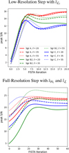 |
Fig. 8 Peak signal-to-noise ratio of the candidate solution of the specified FISTA iteration for the first major cycle of the low- and full-resolution steps, respectively. The full-resolution images were constructed with îℒ set as a low-pass filtered version of the ground-truth image. We observed slightly faster reconstruction speeds for low values of ℓ in the low-reconstruction step, but these configurations are significantly slower in the full-resolution step. It should be noted that although lower values of ℓ improve faster for the low-resolution step, they do not necessarily converge to a better result, as illustrated in the dataset Sgr B2. |
5.3 Comparison to reconstruction without partition of visibilities and to multi-scale CLEAN
We compare our multi-step method to both a single-step method that reconstructs using all visibilities, and to multiscale CLEAN. Figure 9 shows the final reconstructed images and their absolute errors with their respective peak S/Ns in dB for a single-step reconstruction using all the visibilities Vℒ ∪ Vℋ , multi-scale CLEAN, and the proposed multi-step reconstructions using first Vℒ and then Vℋ. We more aggressively increased λℒ for the multi-step reconstructions compared to what was stated in Sect. 5, as we found this to remove wave-like artifacts that were occurring on the edges of the images. Specifically, we used  . Although the three methods achieved comparable peak S/Ns, we also found there to be a visual difference in terms of their error images. In particular, we found multi-scale CLEAN to perform better at reconstructing the larger-scale features but worse at reconstructing the smaller scales, which the other two methods reconstruct to a similar level of accuracy.
Figure 10 shows the progression of all three methods across major-cycle iterations, with ten major-cycles for both the singlestep method and multi-scale CLEAN and five low-resolution (major cycles 1–5) and five full-resolution (major cycles 6–10) major cycles for our method. We found that the three methods obtained reconstructions with comparable peak S/Ns after six to seven major cycles, with the single-step method and multiscale CLEAN sometimes improving after this point, whereas our multi-step method does not. The main reason for this is that the other two methods have double the number of major cycles to improve the larger scale features, which dominate the peak S/N. In practice, as our method only improves for one to two major cycles in the full-resolution step, we can allocate more major cycles to the low-resolution step in order to achieve better peak S/Ns at the end of ten major cycles. Another important aspect to note is that the major cycles for our multi-step method are less computationally expensive, as less visibilities need to be (de)gridded. Thus, reconstructions for the same number of major cycles should be faster to compute when compared to the other tested methods. However, thorough benchmarking is required to determine the actual amount of speedup.
We also found the total number of FISTA iterations required by the single-step method to be comparable to the multi-step one. Figure 11 shows the reconstruction speed across FISTA iterations for the single-step method during the first major cycle. We observed that the single-step method requires two to three times less FISTA iterations compared to the full-resolution step in the multi-step method, and it requires roughly 1.5 times more than the low-resolution step. This, coupled with there being more major-cycle iterations needed for the low-resolution step than the full, means that the total number of FISTA iterations between the single and multi-step approaches roughly equalize, leading to comparable costs for each major cycle.
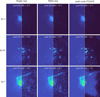 |
Fig. 9 Reconstructed images (left) and absolute error images (right) for our multi-step method (ℓ = 35, δ = 5) using five low-resolution major cycles and five full-resolution major cycles, a single-step all-baselines reconstruction method using ten major cycles, and multi-scale CLEAN using ten major cycles. The corresponding images share scales. Overall, the different methods reconstruct images of comparable peak S/Ns, with multi-scale CLEAN performing better with the larger scales, and the other two methods performing better with the smaller. |
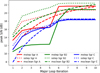 |
Fig. 10 Progression of image reconstruction quality across five low- resolution and five full-resolution major cycles for our proposed multistep method and ten major cycles for a single-step method that reconstructs using all visibilities and multi-scale CLEAN. For our multi-step method, major cycles 1–5 are the low-resolution step, and major cycles 6-10 are the full-resolution step. We found the methods to have comparable peak S/Ns after 6–7 major cycles, with the single-step method and multi-scale CLEAN sometimes improving after this point. It should be noted that the major cycles for the multi-step method are computationally cheaper than the others, as there are less visibilities to (de)grid. |
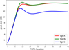 |
Fig. 11 Progression of peak S/N across FISTA iterations for the first major-cycle iteration of the single-step all-baselines reconstruction. Compared to the multi-step method, the convergence is faster than the full-resolution step but slower than the low-resolution step. |
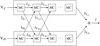 |
Fig. 12 Example workflow of how parallelism will work with our proposed method. We look to reconstruct full-resolution images in parallel, achieved by sharing the deconvolved residuals across different nodes after each major cycle, denoted as MC in the figure. A low and high- resolution image are produced after the first major cycle, denoted as |


6 Conclusion and future work
6.1 Conclusions
This paper proposes a radio-interferometric imaging framework that allows for partitioning of visibilities by baseline. This has several advantages over previous approaches that require all baselines to be treated simultaneously in that (1) it alleviates memory concerns, as not all baselines need to be gridded simultaneously; (2) it allows for more flexible distribution of visibility data in a cluster; and (3) it enables progressive reconstruction.
We have presented our method in the context of sparsity regularized convex optimization problems with over-redundant wavelet dictionaries and compared it to a single-step approach in the same framework that processes all baselines simultaneously without partitioning as well as to RASCIL’s implementation of multi-scale CLEAN. In addition to a better data distribution, we find our method reconstructs images of similar quality in roughly the same total number of major cycles, assuming that the low- and full-resolution major cycles for our method are counted separately. This is promising for the overall computational costs, as each major-cycle iteration for our method should be cheaper to compute given that we only process a subset of the visibilities.
The main drawback to our proposed method is that it creates a secondary data product, the low-resolution image îℒ used in the full-resolution reconstruction step. This could be a significant stumbling block, especially in the context of the SKA, where storage costs are a concern. However, this can be alleviated by reconstructing in Equation (4) a down-sampled image according to the partition configuration. This smaller-sized image can then be incorporated into the second data fidelity term of Equation (5) after an appropriate modification of Gℒ and the addition of a decimation operator to Wα.
6.2 Future work
There are several avenues to extending our work. One natural extension is studying how our framework performs with more than two steps, which will afford us information on the limit of partitioning by baseline. Furthermore, we are also looking to optimize our implementation in order to obtain quantitative results with regard to computational costs.
In addition, we are looking to incorporate parallelism into our framework. This can be done by reconstructing two fullresolution images simultaneously (rather than a low-resolution image first and then a full-resolution one), which can be achieved by sharing the deconvolved residuals between nodes after every major cycle. Thus, low- and high-resolution images are reconstructed after the first major cycle and full-resolution images from then on. The full-resolution reconstructions from each node can then be combined to produce the final reconstructed image. An example workflow of this can be seen in Fig. 12.
Lastly, although we present our method in the framework of sparsity regularized convex optimization problems, the central underlying idea is general. For this reason, an avenue of future research would be to investigate extending this method to other reconstruction frameworks, such as CLEAN.
Acknowledgements
This work was supported by DARK-ERA (ANR-20-CE46- 0001-01).
Appendix A Preliminary simulations for parameter selection
Our proposed method requires knowing the regularization parameters λℒ and λℋ , as well as the wavelet dictionary W. This appendix discusses our preliminary experiments to determine these.
A.1 Choice of wavelet dictionary
The choice of the wavelet dictionary can greatly affect the quality of the reconstruction. We experimented with using both a concatenation of the first 8 Daubechies (Daubechies 1992) wavelets and Isotropic Undecimated Wavelet Transform (IUWT) (Starck et al. 2007). Figure A.1 shows a comparison between reconstructed images of both dictionaries when using a single-step L1 regularized reconstruction of the Sgr A database when simultaneously processing all visibilities Vℒ∪ℋ.
We found that both dictionaries exhibited artifacts, with Daubechies exhibiting various tiling effects and discontinuities at larger values of λ, and IUWT exhibiting false sources. However, we found that the Daubechies dictionary allowed for both better reconstruction of large-scale structures, and was more robust to changes in λ, as shown in Fig. A.2, supporting our use for it in our experiments. A possible reason for why IUWT performs worse for our test cases is due to its isotropic nature, which performs poorly with the large-scale anisotropic features prevalent in our datasets, such as the gas clouds.
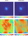 |
Fig. A.1 Reconstructed images from the Sgr A full visibilities dataset using both a concatenated dictionary of the first eight Daubechies wavelets (right) and IUWT (left) wavelets for a single major iteration using a single-step method that reconstructs with Vℒ ∪ Vℋ. Provided below are the error images against the ground truth, which show that the Daubechies dictionary is able to better reconstruct the large-scale gas structures. We use a log10 scale to better illustrate the structural differences for the error images. |
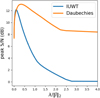 |
Fig. A.2 peak S/N (dB) of different λ values for the first major cycle when performing a single-step reconstruction using Vℒ ∪ Vℋ for Sgr A using a concatenation of the first eight Daubechies wavelets and IUWT wavelets. We found Daubechies wavelets better reconstruct the large- scale features, as evidenced by the higher peak S/N values, and to also be more robust to changes of λ, having a larger range of values that work well. |
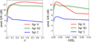 |
Fig. A.3 Reconstruction quality of images for our three datasets for different values of λ. The left image shows peak S/N in dB versus λ for the first major cycle for our three initial datasets, illustrating the different ideal values across different objects. This becomes less problematic when normalizing by the L2-norm of the dirty image ||ĩ1||2. As shown on the right, |

A.2 The regularization parameter λ
The selection of the ideal regularization parameters  and
and  depends on a slew of variables, such as the strength and nature of the object being imaged, the amount of noise present in the measurements, and the wavelet dictionary used. We perform preliminary experiments to determine these – deriving a general strategy is outside the scope of this work.
All our preliminary experiments are done with the singlestep L1 regularized method that reconstructs with Vℒ ∪ Vℋ , and evaluate λ. We generalize the findings here to λℒ and λℋ for our multi-step method, as the nature of reconstructed images are similar, albeit at different resolutions. Finally, as discussed in the previous section, we used a concatenation of the first eight Daubechies wavelets as our dictionary.
Figure A.3 shows the results for our three datasets for the first major cycle. The left image plots λ as the x-axis, whereas the right plots the normalized value  . We found that normalization allows for the well performing regions to line-up, implying that we can pass a constant value for our simulations without the need for dataset specific parameter tuning. We found
  to work well for the single-step reconstructions, and
  to work well for our multi-step method.
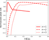 |
Fig. A.4 Normalized peak S/N against |


We hypothesize that the larger ideal values for the low- resolution step can be explained by there being less frequencies, ergo needing less wavelet coefficients. On the other hand, the larger values for the full-resolution step could be explained by the low-resolution data fidelity term biasing the reconstruction to have less noise and fine-scale features, which also increases the sparsity of the wavelet coefficients.
We also evaluate how λ changes across major-cycle iterations, which is necessary as the nature of residual images ĩn changes. Figure A.4 illustrates the behavior of  across three different major cycles for the Sgr A dataset. We normalize by the maximum peak S/N obtained for each respective major cycle for easier comparison. The ground truth images we use to compute the peak S/N are defined as I − ∑N în, where I is the initial ground truth, and în is the best reconstructed image among the different
  values for the nth major cycle.
It can be seen that the ideal values for  generally increases as we progress through the major-cycle iterations. This is expected as the residual images are increasingly dominated by noise, necessitating larger values of
  to suppress it. However, care needs to be taken not to increase it too aggressively, as this will lead to all fine scale features being ignored, as shown in Fig. A.5. We found that multiplying
  by 2n for the nth major cycle provides a good trade-off between the two.
Finally, we would like to note that for the full-resolution reconstruction, a less aggressive regularization parameter λ does allow for further reduction of the residual in latter major cycles. However, we found this to overfit to noise, reducing the peak S/N of the overall reconstruction. Figure A.6 illustrates this for the Sgr A ℓ = 20, δ = 5 dataset.
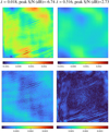 |
Fig. A.5 Reconstructed images as well as their absolute errors of the Sgr C dataset for the second major cycle residual image ĩ2 using the single-step method, with a lower (left) and higher (right) λ. The larger λ has a better peak S/N, as it reduces the error on a large scale, but it is not able to reconstruct any of the finer-scale details. |
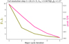 |
Fig. A.6 L2-norm of the residual and the peak S/N of the reconstructed image for the full-resolution step across major cycles. A less aggressive regularization parameter was used here, which results in further reduction of the residual in the later major cycles. However, this also detracts from the peak S/N, as the reconstructed image is overfits the noise. |
References
- Barnett, A. H., Magland, J., & Af Klinteberg, L. 2019, SISC, 41, C479 [CrossRef] [Google Scholar]
- Beck, A., & Teboulle, M. 2009, SIIMS, 2, 183 [CrossRef] [Google Scholar]
- Bezanson, J., Edelman, A., Karpinski, S., & Shah, V. B. 2017, SIAM Rev., 59, 65 [Google Scholar]
- Bhatnagar, S., Cornwell, T. J., Golap, K., & Uson, J. M. 2008, A&A, 487, 419 [NASA ADS] [CrossRef] [EDP Sciences] [Google Scholar]
- Cai, X., Pratley, L., & McEwen, J. D. 2019, MNRAS, 485, 4559 [CrossRef] [Google Scholar]
- Candes, E. J., Romberg, J., & Tao, T. 2006, IEEE Trans. Inf. Theory, 52, 489 [CrossRef] [Google Scholar]
- Candès, E. J., Eldar, Y. C., Needell, D., & Randall, P. 2011, ACHA, 31, 59 [Google Scholar]
- Carrillo, R. E., McEwen, J. D., & Wiaux, Y. 2014, MNRAS, 439, 3591 [Google Scholar]
- Cornwell, T. J. 2008, IEEE J-STSP, 2, 793 [NASA ADS] [Google Scholar]
- Cornwell, T. J., & Perley, R. A. 1992, A&A, 261, 353 [NASA ADS] [Google Scholar]
- Cornwell, T. J., Golap, K., & Bhatnagar, S. 2008, IEEE J-STSP, 2, 647 [NASA ADS] [Google Scholar]
- Cornwell, T. J., Voronkov, M. A., & Humphreys, B. 2012, SPIE, 8500, 186 [Google Scholar]
- Cornwell, T. J., Wortmann, P., Nikolic, B., Wang, F., & Stolyarov, V. 2020, Radio Astronomy Simulation, Calibration and Imaging Library [Google Scholar]
- Dabbech, A., Ferrari, C., Mary, D., et al. 2015, A&A, 576, A7 [CrossRef] [EDP Sciences] [Google Scholar]
- Daubechies, I. 1992, Ten Lectures on Wavelets (SIAM) (Berlin: Springer) [CrossRef] [Google Scholar]
- Donoho, D. L. 2006, IEEE Trans. Inf. Theory, 52, 1289 [CrossRef] [Google Scholar]
- Garsden, H., Girard, J. N., Starck, J.-L., et al. 2015, A&A, 575, A90 [CrossRef] [EDP Sciences] [Google Scholar]
- Gheller, C., Taffoni, G., & Goz, D. 2023, RAS Tech. Instrum., 2, 91 [NASA ADS] [CrossRef] [Google Scholar]
- Heywood, I., Rammala, I., Camilo, F., et al. 2022, ApJ, 925, 165 [NASA ADS] [CrossRef] [Google Scholar]
- Högbom, J. A. 1974, A&AS, 15, 417 [Google Scholar]
- Jiang, M., Girard, J. N., Starck, J.-L., Corbel, S., & Tasse, C. 2015, in EUSIPCO (IEEE), 1646 [Google Scholar]
- Labate, M. G., Waterson, M., Alachkar, B., et al. 2022, J. Astron. Telesc. Instrum. Syst., 8, 011024 [NASA ADS] [CrossRef] [Google Scholar]
- Lauga, G., Repetti, A., Riccietti, E., et al. 2024, arXiv e-prints [arXiv:2403.13385] [Google Scholar]
- Mallat, S. G., & Zhifeng, Z. 1993, IEEE Trans. Signal Process, 41, 3397 [CrossRef] [Google Scholar]
- Merry, B. 2016, A&C, 16, 140 [NASA ADS] [Google Scholar]
- Monnier, N., Guibert, D., Tasse, C., et al. 2022, in Proceedings of the 2022 IEEE SIPS [Google Scholar]
- Offringa, A. R., McKinley, B., Hurley-Walker, N., et al. 2014, MNRAS, 444, 606 [Google Scholar]
- Onose, A., Carrillo, R. E., Repetti, A., et al. 2016, MNRAS, 462, 4314 [NASA ADS] [CrossRef] [Google Scholar]
- Ord, S. M., Mitchell, D. A., Wayth, R. B., et al. 2010, PASP, 122, 1353 [CrossRef] [Google Scholar]
- Pratley, L., Johnston-Hollitt, M., & McEwen, J. D. 2019a, ApJ, 874, 174 [NASA ADS] [CrossRef] [Google Scholar]
- Pratley, L., McEwen, J. D., d’Avezac, M., et al. 2019b, arXiv e-prints [arXiv: 1903.04502] [Google Scholar]
- Rau, U., & Cornwell, T. J. 2011, A&A, 532, A71 [NASA ADS] [CrossRef] [EDP Sciences] [Google Scholar]
- Romein, J. W. 2012, in Proceedings of the 26th ACM ICS, 321 [Google Scholar]
- Smirnov, O. M. 2011, A&A, 527, A106 [NASA ADS] [CrossRef] [EDP Sciences] [Google Scholar]
- Starck, J.-L., Fadili, J., & Murtagh, F. 2007, IEEE Trans. Image Process., 16, 297 [Google Scholar]
- Swart, G. P., Dewdney, P., & Cremonini, A. 2022, J. Astron. Telesc. Instrum. Syst., 8, 011021 [NASA ADS] [CrossRef] [Google Scholar]
- Tasse, C., Hugo, B., Mirmont, M., et al. 2018, A&A, 611, A87 [NASA ADS] [CrossRef] [EDP Sciences] [Google Scholar]
- Van Der Tol, S., Veenboer, B., & Offringa, A. R. 2018, A&A, 616, A27 [NASA ADS] [CrossRef] [EDP Sciences] [Google Scholar]
- Van Weeren, R. J., Williams, W. L., Hardcastle, M. J., et al. 2016, ApJS, 223, 2 [CrossRef] [Google Scholar]
- Veenboer, B., Petschow, M., & Romein, J. W. 2017, in IEEE IPDPS, 545 [Google Scholar]
- Wiaux, Y., Jacques, L., Puy, G., Scaife, A. M. M., & Vandergheynst, P. 2009, MNRAS, 395, 1733 [NASA ADS] [CrossRef] [Google Scholar]
- Ye, H., Gull, S. F., Tan, S. M., & Nikolic, B. 2022, MNRAS, 510, 4110 [NASA ADS] [CrossRef] [Google Scholar]
All Tables
All Figures
|
Fig. 1 High-level overview of the radio-interferometric pipeline. A reconstructed image în is compared to the measurements v in the (de)gridding step, which outputs the difference in the spatial domain ĩn. This is passed to the reconstruction algorithm, which generates the next estimate în+1 by deconvolving the residual image ĩn and adding it to în. |
| In the text | |
|
Fig. 2 Full set of visibilities partitioned according to the domains. The domain ℒ (orange) contains the short baseline visibilities, and ℋ (green) contains the long baseline visibilities. These are not mutually exclusive but rather have an overlap region indicated in cyan and defined using ℓ, which is the middle of ℒ ∩ ℋ, and δ, the half-width of ℒ ∩ ℋ. |
| In the text | |
|
Fig. 3 Radial frequency response of Gℋ and Gℒ for σ2 = 1 and η2 = 1.2. |
| In the text | |
|
Fig. 4 Ground truth images of our three datasets obtained by cutting out and tapering sections of the 1.28 GHz Meerkat galactic center mosaic (Heywood et al. 2022). The images are 512 × 512 pixels in size with a resolution of 1.1″ per pixel. The UV coverage for our simulated datasets is shown at the bottom right. The same coverage was used for all three datasets. |
| In the text | |
|
Fig. 5 Visualization of partition configuration parameters δ and ℓ used for our datasets. We only show δ for ℓ = 55 in this figure to avoid clutter. The combinations of the three values of δ and three values of ℓ result in nine different partitioning configurations per dataset. |
| In the text | |
|
Fig. 6 Dirty images |
| In the text | |
|
Fig. 7 Progression of peak S/N of reconstructed images for various partitioning configurations across the major cycles for both the low- and full-resolution reconstruction steps. peak S/Ns have been normalized by the maximum value of each configuration to allow for easier comparison. An exponential scale is used for the bottom image to better illustrate the differences between the different configurations. We fixed δ = 5 here, as we found it does not greatly impact the results. |
| In the text | |
|
Fig. 8 Peak signal-to-noise ratio of the candidate solution of the specified FISTA iteration for the first major cycle of the low- and full-resolution steps, respectively. The full-resolution images were constructed with îℒ set as a low-pass filtered version of the ground-truth image. We observed slightly faster reconstruction speeds for low values of ℓ in the low-reconstruction step, but these configurations are significantly slower in the full-resolution step. It should be noted that although lower values of ℓ improve faster for the low-resolution step, they do not necessarily converge to a better result, as illustrated in the dataset Sgr B2. |
| In the text | |
|
Fig. 9 Reconstructed images (left) and absolute error images (right) for our multi-step method (ℓ = 35, δ = 5) using five low-resolution major cycles and five full-resolution major cycles, a single-step all-baselines reconstruction method using ten major cycles, and multi-scale CLEAN using ten major cycles. The corresponding images share scales. Overall, the different methods reconstruct images of comparable peak S/Ns, with multi-scale CLEAN performing better with the larger scales, and the other two methods performing better with the smaller. |
| In the text | |
|
Fig. 10 Progression of image reconstruction quality across five low- resolution and five full-resolution major cycles for our proposed multistep method and ten major cycles for a single-step method that reconstructs using all visibilities and multi-scale CLEAN. For our multi-step method, major cycles 1–5 are the low-resolution step, and major cycles 6-10 are the full-resolution step. We found the methods to have comparable peak S/Ns after 6–7 major cycles, with the single-step method and multi-scale CLEAN sometimes improving after this point. It should be noted that the major cycles for the multi-step method are computationally cheaper than the others, as there are less visibilities to (de)grid. |
| In the text | |
|
Fig. 11 Progression of peak S/N across FISTA iterations for the first major-cycle iteration of the single-step all-baselines reconstruction. Compared to the multi-step method, the convergence is faster than the full-resolution step but slower than the low-resolution step. |
| In the text | |
|
Fig. 12 Example workflow of how parallelism will work with our proposed method. We look to reconstruct full-resolution images in parallel, achieved by sharing the deconvolved residuals across different nodes after each major cycle, denoted as MC in the figure. A low and high- resolution image are produced after the first major cycle, denoted as |
| In the text | |
|
Fig. A.1 Reconstructed images from the Sgr A full visibilities dataset using both a concatenated dictionary of the first eight Daubechies wavelets (right) and IUWT (left) wavelets for a single major iteration using a single-step method that reconstructs with Vℒ ∪ Vℋ. Provided below are the error images against the ground truth, which show that the Daubechies dictionary is able to better reconstruct the large-scale gas structures. We use a log10 scale to better illustrate the structural differences for the error images. |
| In the text | |
|
Fig. A.2 peak S/N (dB) of different λ values for the first major cycle when performing a single-step reconstruction using Vℒ ∪ Vℋ for Sgr A using a concatenation of the first eight Daubechies wavelets and IUWT wavelets. We found Daubechies wavelets better reconstruct the large- scale features, as evidenced by the higher peak S/N values, and to also be more robust to changes of λ, having a larger range of values that work well. |
| In the text | |
|
Fig. A.3 Reconstruction quality of images for our three datasets for different values of λ. The left image shows peak S/N in dB versus λ for the first major cycle for our three initial datasets, illustrating the different ideal values across different objects. This becomes less problematic when normalizing by the L2-norm of the dirty image ||ĩ1||2. As shown on the right, |
| In the text | |
|
Fig. A.4 Normalized peak S/N against |
| In the text | |
|
Fig. A.5 Reconstructed images as well as their absolute errors of the Sgr C dataset for the second major cycle residual image ĩ2 using the single-step method, with a lower (left) and higher (right) λ. The larger λ has a better peak S/N, as it reduces the error on a large scale, but it is not able to reconstruct any of the finer-scale details. |
| In the text | |
|
Fig. A.6 L2-norm of the residual and the peak S/N of the reconstructed image for the full-resolution step across major cycles. A less aggressive regularization parameter was used here, which results in further reduction of the residual in the later major cycles. However, this also detracts from the peak S/N, as the reconstructed image is overfits the noise. |
| In the text | |
Current usage metrics show cumulative count of Article Views (full-text article views including HTML views, PDF and ePub downloads, according to the available data) and Abstracts Views on Vision4Press platform.
Data correspond to usage on the plateform after 2015. The current usage metrics is available 48-96 hours after online publication and is updated daily on week days.
Initial download of the metrics may take a while.