| Issue |
A&A
Volume 696, April 2025
|
|
|---|---|---|
| Article Number | A216 | |
| Number of page(s) | 16 | |
| Section | Numerical methods and codes | |
| DOI | https://doi.org/10.1051/0004-6361/202554072 | |
| Published online | 25 April 2025 | |
DeepShape: Radio weak-lensing shear measurements using deep learning
Université Côte d’Azur,
Observatoire de la Côte d’Azur, CNRS,
06000 Nice,
France
★ Corresponding author; priyamvad.tripathi@oca.eu
Received:
7
February
2025
Accepted:
29
March
2025
Context. The advent of upcoming radio surveys, such as those enabled by the SKA Observatory, will provide the desired sensitivity and resolution required for weak-lensing studies. However, current shape and shear measurement methods are mostly tailored for optical surveys. The development of novel techniques to facilitate weak-lensing measurements in the radio waveband is thus needed.
Aims. There are a few algorithms for shape measurement in the radio waveband. However, these are either computationally intensive or fail to achieve the accuracy required for future surveys. In this work, we present a supervised deep learning framework, dubbed DeepShape, that measures galaxy shapes with the necessary precision while minimizing computational expenses.
Methods. DeepShape is made of two modules. The first module is a plug-and-play (PnP) image reconstruction algorithm based on the half-quadratic splitting method (HQS), dubbed HQS-PnP, which reconstructs images of isolated radio galaxies. The second module is a measurement network that predicts galaxy shapes using the point spread function and reconstructed image pairs.
Results. We test our framework on a simulated radio data set based on the SKA-MID AA4 array configuration. The HQS-PnP algorithm outperforms the standard multiscale CLEAN algorithm across several tested metrics. DeepShape recovers galaxy shapes with an accuracy comparable to the leading radio shape measurement method, RadioLensfit, while significantly reducing the prediction time from ~4 minutes to ~220 milliseconds. We also demonstrate DeepShape’s applicability to shear measurements and recover shear estimates with an additive bias meeting SKA-MID requirements. Although the multiplicative shear bias is an order of magnitude higher than the required level, it can be mitigated using a shear measurement calibration technique, such as applying quality cuts.
Key words: gravitational lensing: weak / methods: data analysis / techniques: image processing / techniques: interferometric / radio continuum: galaxies
© The Authors 2025
 Open Access article, published by EDP Sciences, under the terms of the Creative Commons Attribution License (https://creativecommons.org/licenses/by/4.0), which permits unrestricted use, distribution, and reproduction in any medium, provided the original work is properly cited.
This article is published in open access under the Subscribe to Open model. Subscribe to A&A to support open access publication.
1 Introduction
Weak gravitational lensing is a phenomenon that describes the deflection of light from background sources by the tidal fields of an inhomogeneous matter distribution along the line of sight. In the context of large-scale structures, this results in a coherent deformation of the observed shapes of the background galaxies known as cosmic shear. Cosmic shear is a powerful tool for probing the total mass distribution and studying the relationship between dark matter and baryonic matter. Additionally, it can be used to study the growth of structure and the nature of dark energy (see Kilbinger 2015 for a recent review).
Shear contributes only to a small part of the overall galaxy shape, necessitating highly precise shape measurements and large number statistics to reliably extract the shear signal. As a result, observational detections of shear signal have mainly been performed in the optical waveband (Tyson et al. 1990; Bacon et al. 2000; Wittman et al. 2000) owing to their higher resolution, better sensitivity, higher background galaxy number density, and wider area coverage than radio surveys. Nevertheless, cosmic shear signals have previously been detected in the radio waveband, albeit with a lower detection significance (Chang et al. 2004; Patel et al. 2010; Harrison et al. 2020). Upcoming radio surveys, such as those provided by the SKA Observatory (Weltman et al. 2020), are set to deliver radio datasets of starforming galaxies with the sensitivity and resolution necessary for weak-lensing studies. However, these advancements also bring a host of new challenges. Radio measurements are obtained in the Fourier space of the image domain, known as the visibility domain. This leads to different systematics compared to the optical waveband. As a result, there is a need to reassess existing shape measurement and bias calibration techniques, as they are optimized for optical datasets (Patel et al. 2015).
The traditional approach to shear measurement involves two steps: first, an initial shear estimate is obtained by calculating the ensemble average of the shapes within a galaxy population; second, the estimated shear is calibrated using parameters derived from simulated observations. The state-of-the-art method, METACALIBRATION (Sheldon & Huff 2017), estimates shear bias by applying known shear signals to the original image, a bias correction is then applied to the original measurement. Applying this method in the radio waveband would be computationally very expensive owing to the high computational costs of gridding/de-gridding operations as well as image reconstruction. Another potential approach is to use deep learning-based methods that directly measure shapes from dirty images with minimal computational costs (Ribli et al. 2019; Zhang et al. 2024). However, applying these methods to the radio waveband presents challenges due to the poorer quality of dirty images. This degradation arises from two factors: first, the point spread function (PSF) in the radio waveband typically has larger sidelobes than in the optical waveband; second, the image domain noise is highly correlated for radio waveband observations. The state-of-the-art radio shear measurements are based on a parametric model directly fitted in the Fourier domain (Chang et al. 2004; Rivi et al. 2016; Rivi & Miller 2022). However, these methods tend to be slow due to the large dimensions of the visibility space and could also lead to model bias (Voigt & Bridle 2010).
As an initial step toward developing a properly calibrated shear field estimator, we present a supervised deep learning framework named DeepShape, designed to predict the shapes of isolated radio galaxies from their dirty images and associated PSFs. DeepShape is made of two modules. The first module uses a plug-and-play (PnP) algorithm based on the half-quadratic splitting (HQS) method to reconstruct galaxy images. The second module is a measurement network trained to predict galaxy shapes from the reconstructed image-PSF pairs. The measurement network is divided into two branches: one is a feature extraction branch, which employs an equivariant convolutional neural network (CNN) to extract features from the reconstructed image, while the other is a pre-trained encoder block that compresses the PSF into a low-dimensional code, accounting for PSF-dependent errors. The outputs of both branches are combined and passed through a dense layer block to predict the ellipticity.
The paper is organized as follows: we provide a brief overview of the radio-interferometric imaging process and weak-lensing studies in Sect. 2; we describe our image reconstruction algorithm and measurement network in Sect. 3 along with a short summary of state-of-the-art shape measurement methods in the radio waveband; Sect. 4 describes the details of our simulations followed by a description of the training/testing datasets in Sect. 5; we present and discuss our results in Sect. 6; and finally we list the conclusions and discuss possible avenues for future work in Sect. 7.
2 Theory
2.1 Radio-interferometric imaging
Radio interferometers measure sky brightness in the Fourier domain, known as visibility space. The visibilities represent the correlated response of an antenna pair to the electric field integrated over a time period and frequency band (Thompson et al. 2017). The measurement process is given by:
 (1)
(1)
where (u, v, w) are relative antenna pair positions, (l, m) are direction cosines, V(u, v, w) are the observed visibilities, IT (l, m) is the sky brightness distribution and nuvw represents an additive instrumental noise.
Assuming a small field of view (l2 + m2 → 0), Eq. (1) simplifies to a two-dimensional Fourier transform, which can be further approximated as a fast Fourier transform (FFT) on a regular grid, followed by a degridding operation:
 (2)
(2)
where iT is the true sky image, u are the measured visibilities, F is the FFT, and G† is the degridding operator responsible for extrapolating the regular gridded visibilities to their original irregular positions. For the sake of brevity, we eliminate the coordinates from iT (l, m), u(u, v, w) and n(u, v, w). Equation (2) is then inverted to get a so-called “dirty” image iD:
 (3)
(3)
where F† is the inverse FFT and G is the gridding operator responsible for interpolating the irregular visibilities to regular gridded positions. The dirty image exhibits artifacts due to incomplete Fourier sampling, omission of the w-term, gridding errors, and correlated noise in the image space. Radiointerferometric imaging aims to correct for these artifacts and reconstruct an image that is usable for science (CASA Team 2022).
Standard reconstruction methods rewrite Eq. (3) as a convolution:
 (4)
(4)
where H ≡ F† Diag(GG†)F is the convolution operator, h is the dirty beam or PSF, * corresponds to convolution operation and  is the correlated image-space noise. Equation (4) can then be solved by using a standard deconvolution method, such as CLEAN (Högbom 1974) or its variants, to produce an image estimate. CLEAN is effective for reconstructing compact sources and is widely used due to its simplicity and computational efficiency. However, it struggles with extended emission, can introduce non-physical negative flux regions in the reconstructed image, and is sensitive to user-defined parameters which must be carefully tuned based on the specific imaging problem (Arras et al. 2021; Terris et al. 2022; Müller & Lobanov 2023).
Even with a highly effective deconvolution algorithm, the reconstructed image inevitably contains artifacts because Eq. (9) does not account for the w-term and gridding errors. The fidelity of the reconstructed image,  , can be evaluated by computing the residual image, iR, defined as:
 (5)
(5)
If iR still contains structural information, it indicates that the reconstruction is incomplete. In such cases, the residual image is deconvolved again to extract additional corrections, which are then added to the initial reconstruction. This iterative process, known as the major-minor loop reconstruction (CASA Team 2022), continues until the residual image is reduced to noise. This approach is particularly critical for wide-field imaging, where the effects of the w-term and gridding errors become significant. However, it is a time-consuming process due to the high computational cost of gridding and degridding operators.
2.2 Weak-lensing formalism
The weak-lensing signal is primarily carried by faint starforming galaxies (SFGs) (Zhang et al. 2015). The radiation emitted by these galaxies is deflected by the intervening largescale structures between the observer and the galaxy. This phenomenon can be parametrized using the Jacobi matrix A of the 2D gravitational potential:
 (6)
(6)
where κ is the scalar convergence which quantifies the isotropic magnification of the source. The shear γ = (γ1, γ2) is a spin-2 field that quantifies the anisotropic stretching of the galaxy image perpendicular to the line of sight (Seitz & Schneider 1997).
The main observable effect of weak-lensing is the shear, which perturbs the observed shape of galaxies. This effect can be approximated by:
 (7)
(7)
where ϵ = (ϵ1, ϵ2) is the observed galaxy ellipticity and  is the intrinsic source ellipticity. Shear constitutes only a small portion of the galaxy’s overall ellipticity, ||γ|| ≪ ||ϵ||. In the absence of intrinsic alignment of the background galaxies,
 ![${\mathds{E}[\bm{\epsilon}^I] = 0}$](/articles/aa/full_html/2025/04/aa54072-25/aa54072-25-eq11.png) , the shear can be inferred by calculating an average of galaxy ellipticities. However, these measurements tend to be biased due to various systematics introduced in the observation process. This bias is conventionally defined by a linear model (Heymans et al. 2006; Huterer et al. 2006) consisting of a multiplicative bias Mα and an additive bias Cα:
, the shear can be inferred by calculating an average of galaxy ellipticities. However, these measurements tend to be biased due to various systematics introduced in the observation process. This bias is conventionally defined by a linear model (Heymans et al. 2006; Huterer et al. 2006) consisting of a multiplicative bias Mα and an additive bias Cα:
 (8)
(8)
where <ϵα> is the ensemble-averaged ellipticity measurements and α corresponds to the two shape components.
The bias parameters Mα and Cα have nontrivial dependence on the properties of the galaxy (such as size, magnitude, intrinsic ellipticity), redshift, PSF, shape measurement algorithm, etc. An upper limit on the bias parameters can be calculated such that the cosmological results are dominated by statistical uncertainties rather than systematic errors. This limit depends on factors such as the sky area, median redshift, and number density of the survey. The bias requirements for the SKA-MID survey specify that |Mα| < 6.7 10−3 and Cα < 8.2 10−4 (Patel et al. 2015) and the uncertainties on the bias parameters should be of the same order.
3 Methodology
We propose a supervised deep learning framework, dubbed DeepShape, comprising two modules. The first module is a plug-and-play (PnP) algorithm based on the half-quadratic splitting (HQS) method to reconstruct a galaxy image from a given dirty image and PSF pair. The second module, a measurement network, estimates galaxy shapes based on the PSF and the reconstructed image. Overall, DeepShape takes two inputs: a dirty image iD and the associated PSF h and outputs an ellipticity estimate  .
.
3.1 Image reconstruction
For image reconstruction, we utilize a deep learning-based PnP algorithm inspired by the work of Zhang et al. (2020). The idea behind PnP algorithms is to split the image restoration problem into two sub-tasks: a convex optimization problem which can be solved using traditional iterative methods like the proximal gradient descent method (Parikh & Boyd 2014) and a regularization task that is performed by pre-trained deep learning-based denoisers, such as UNet (Ronneberger et al. 2015). PnP algorithms have demonstrated state-of-the-art reconstruction performance across various image processing applications, including biomedical imaging, microscopy, and video deblurring (Sun et al. 2019; Xu et al. 2020; Liu et al. 2021). We opted for a PnP scheme rather than an unfolded scheme (Ongie et al. 2020) because the latter is trained for a specific PSF. In radio astronomy, however, the PSF varies based on the pointing direction and the galaxy’s position relative to the pointing center. This variability renders unfolded deconvolution algorithms impractical for radio imaging reconstructions.
The deconvolution equation given by Eq. (9), can be formulated as an optimization problem:
 (9)
(9)
where H is the convolution operator, σ is the RMS image noise, Φ is the regularization function that represents the log-prior on iT and λ ∈ (0, ∞) is the regularization weight. The ||iD - Hi||2/2σ2 term is a data-fidelity term that guarantees the solution accords with the degradation process, while the λΦ(i) term enforces desired properties of the output; and λ acts as trade-off between the fidelity and regularization strength. Equation (9) can then be reformulated as a constrained optimization problem by introducing an auxiliary variable z:
 (10)
(10)
The constraint can be relaxed by minimizing the loss function:
 (11)
(11)
where μ ∈ (0, ∞) is a penalty term that needs to be tuned. μ dictates the balance between data fidelity and the auxiliary variable update and thus influences the convergence speed and the stability of the solution. This approach is known as the HQS method (Nikolova & Ng 2005). This formulation decouples the fidelity term from the regularization term, resulting in two subproblems that can be solved iteratively as follows:
 (12a 12b)
Here, the fixed penalty term μ is replaced with a monotonically increasing sequence μk. This adjustment, enables a gradual reduction in denoising strength with each iteration, resulting in faster convergence (Hurault et al. 2024). Equation (12a) is a standard deconvolution with a Tikhonov regularization and has a fast closed-form solution:
 (13)
(13)
Eq. (12b) is a denoising problem that can be solved by using a CNN denoiser  that is pre-trained to denoise images ik+1 with Gaussian noise RMS
  :
:
 (14)
(14)
If we take the Fourier transform of ik+1 in Eq. (13) and calculate the information in the  -th frequency bin, we get:
=\frac{[\Delta^\dagger](\Tilde{n})[F\bm{i}_D](\Tilde{n})+\mu_k\sigma^2[F\bm{z}_k](\Tilde{n})}{[\Delta^\dagger\Delta](\Tilde{n})+\mu_k\sigma^2},](/articles/aa/full_html/2025/04/aa54072-25/aa54072-25-eq23.png) (15)
(15)
where △ is the (diagonal) frequency response of the PSF. Now, suppose that no visibilities fall in the frequency bin  , meaning
 =0$](/articles/aa/full_html/2025/04/aa54072-25/aa54072-25-eq25.png) , we get
, we get =[F\bm{z}_{k}](\Tilde{n})$](/articles/aa/full_html/2025/04/aa54072-25/aa54072-25-eq26.png) . Consequently, the missing spatial frequencies are exclusively reconstructed by the neural network.
. Consequently, the missing spatial frequencies are exclusively reconstructed by the neural network.
CNN-based denoisers offer several advantages over analytical methods, such as total variation or Bayesian denoising.
Input: Dirty image iD, PSF operator H, image noise level σ, penalty μk at iteration k for a total of K iterations, regularization strength λ, pre-trained CNN denoiser 
Output: Reconstructed image 
1 Initialize z0 = iD
2 for k= 1, 2,. . . ,K do
3 ik = (H†H + μkσ2I)−1(H†iD + μkσ2 zk−1);
4 
5 end
6 return 
Unlike traditional approaches that rely on models or assumptions about noise, CNNs learn complex, nonlinear, domain-specific patterns directly from data. They are significantly faster, especially for larger datasets, and typically outperform traditional techniques in metrics like Peak Signal-to-Noise Ratio (PSNR) or Structural Similarity Index (SSIM) (Vincent et al. 2008; Zhang et al. 2017). In particular, we use the DRUNet architecture introduced in Zhang et al. (2020), which denoises an image for a given noise level. DRUNet is a “noise-aware” denoiser capable of generalizing across various noise levels without the need for retraining the network for each noise level. This enables us to reuse the same network at each iteration k, while simply adjusting its denoising strength to  .
.
The overall algorithm is summarized in Algorithm 1. Our reconstruction algorithm can be interpreted as the first major cycle in a standard radio imaging process, with the minor cycle replaced by the HQS-PnP algorithm. Since this work focuses only on sources at the phase center, additional major cycles are unnecessary, as demonstrated in Sect. 6.1.
3.2 Shape measurement
We use a measurement network that takes the image reconstructed using the HQS-PnP algorithm along with the corresponding PSF before deconvolution as input and outputs an ellipticity estimate. Our measurement network consists of two branches: a feature extraction branch that processes the reconstructed image  using an E(2)-equivariant CNN block, and an encoder branch that encodes the PSF h to account for any PSF-dependent error.
Feature extraction: Galaxy ellipticity is equivariant to the actions of 2D Euclidean transformations E(2) of galaxy images. For instance, if the image is rotated by a certain angle, the measured ellipticity should also rotate by the same angle. Therefore, a shape measurement method should also be equivariant to the isometries of the ℝ2 plane, including continuous rotations, reflections, and translations. Traditional CNNs are inherently equivariant only to translations but not to rotations and reflections. One way to impose equivariance within the CNN is to use data augmentation techniques, however, this can slow the training process and lacks geometric guarantees of equivariance (Cohen & Welling 2016). A more effective approach is to incorporate equivariance directly into the model architecture using group-steerable CNNs. These equivariant CNNs have been successfully applied to various image processing tasks (Rodriguez Salas et al. 2021; Bengtsson Bernander et al. 2024; Chidester et al. 2019; Lafarge et al. 2020). Recent studies also highlight that equivariant CNNs outperform traditional CNNs for various astrophysical applications. (Scaife & Porter 2021; Pandya et al. 2023; Lines et al. 2024; Tripathi et al. 2024).
An equivariant convolution uses kernel ker(x|w) with weights w at position x expanded in a steerable basis of the E(2) group:
 (16)
(16)
where  are the basis vectors and the kernel weights wℓ(r) have a radial symmetry. This convolution ensures rotational equivariance for discrete rotations of 2π/L (and multiples of 2π/L), where L is a hyperparameter of the network. For our work, we set L = 8. An E(2) equivariant network is created by stacking multiple layers of E(2)-steerable convolutions. This network produces a vector feature map that is equivariant to the actions of the E(2) group:
![\text{N}_{\text{E}(2)}[R_G(\hat{\bm{\imath}})]=R'_G[\text{N}_{\text{E}(2)}(\hat{\bm{\imath}})],](/articles/aa/full_html/2025/04/aa54072-25/aa54072-25-eq35.png) (17)
(17)
where  is the input image, and RG and
  are the representations of the E(2) group acting on 2D images and the vector feature map respectively. For a more detailed mathematical description of steerable CNNs, we refer the reader to Weiler & Cesa (2019). Our feature extraction block consists of three equivariant convolution layers, interspersed with two average pooling layers. We built the equivariant CNN using the Python library escnn (Cesa et al. 2022).
PSF correction: Ideally, the reconstruction process should completely eliminate the effects of the dirty beam from the reconstructed image. However, in practice, reconstruction is rarely perfect, even with the most advanced reconstruction algorithms, and PSF continues to be a significant source of systematics in weak-lensing measurements (Paulin-Henriksson et al. 2008, 2009; Massey et al. 2013). The PSF smears the shape of observed galaxies, causing a multiplicative bias, while an anisotropy in the PSF can lead to an additive bias, which is known as PSF leakage. In the radio waveband, this issue is further exacerbated by the fact that different galaxies have different PSFs depending on the pointing direction and the relative position of the galaxy. This leads to varying PSF systematics across different galaxies. Consequently, an ideal shape measurement method must be capable of removing artifacts induced by any arbitrary PSF.
To address this, we train our network to remove any remaining PSF-related errors in the reconstructed images. First, we train an autoencoder network that encodes the PSF h to a low-dimensional code ζ. This encoded PSF is then concatenated with the extracted features and passed through the final dense layer block. Our autoencoder is based on a standard convolutional encoder-decoder architecture (Goodfellow et al. 2016) and is trained to minimize the mean squared error (MSE):
![\{{\hat{\bm{\theta}}}_{\text{E}},{{\hat{\bm{\theta}}}_{\text{D}}\}= \underset{\{\bm{\theta}_{\text{E}},\bm{\theta}_{\text{D}}\}}{\text{argmin}}~ \mathbb{E}_{\bm{h}}~[\lVert \bm{h}-\hat{\bm{h}}\lVert^2]},](/articles/aa/full_html/2025/04/aa54072-25/aa54072-25-eq38.png) (18)
(18)
where  is the output from the decoder, and {θE,θD} the encoderdecoder architecture parameters. The encoder/decoder block is made up of three sets of 2D convolutional/transposed convolution layers. Each set contains a pair of convolution/transposed layers of the same size.
Full architecture: The measurement network takes two inputs: a reconstructed galaxy image  and the associated PSF h before deconvolution, and outputs an estimated ellipticity
  is passed through the feature extraction block and h is passed through a pre-trained encoder block. The outputs of the two blocks are concatenated and passed through a final dense layer block to predict the ellipticities:
  . The network is trained to minimize the MSE loss:
![\hat{\bm{\theta}}= \underset{\bm{\theta}}{\text{argmin}}~ \mathbb{E}_{(\hat{\bm\imath},{\bm h},\bm{\epsilon}^{\text{true}})} [\lVert{\hat{\bm{\epsilon}}}-\bm{\epsilon}^{\text{true}}\lVert^2],](/articles/aa/full_html/2025/04/aa54072-25/aa54072-25-eq43.png) (19)
(19)
where ϵtrue is the ground truth ellipticity of the simulated galaxy and θ are the model parameters that need to be optimized: parameters of the feature extraction and dense layer blocks. The network architecture is outlined in Fig. 1.
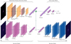 |
Fig. 1 Architecture of the measurement network. The decoder block is shown just for reference and is not a part of the network. All layers have a ReLU activation except the final dense layer, which has a tanh activation. |
3.3 Alternative methods
RadioLensfit: The RadioLensfit method (Rivi et al. 2016) is a parametric model-fitting approach that operates directly in the visibility domain. This bypasses any biases that could be introduced in a standard radio-imaging process. The method assumes that the galaxy brightness can be described as an exponential brightness profile (which corresponds to a Sersic profile of index unity). Under this assumption, the observed visibilities can be modeled using Eq. (1) as:
 (20)
(20)
k = (u, v), I0 is the flux density and rα is the scale length of the emission profile, and  defines the ellipticity of the galaxy profile:
 (21)
(21)
Assuming an additive Gaussian noise, the likelihood of the parameters Θ = {I0, α, l, m, ϵ1, ϵ2} is given by:
![p(\bm{v}_d|\bm{\Theta}) \propto\text{exp}\left[-\frac{(\bm{v}_d-\bm{v}_m)^\dagger \bm{C}^{-1}(\bm{v}_d-\bm{v}_m)}{2}\right].](/articles/aa/full_html/2025/04/aa54072-25/aa54072-25-eq47.png) (22)
(22)
The likelihood is then marginalized over the nuisance parameters – {I0, α, l, m} – using appropriate priors. The marginalized likelihood is then sampled on the ellipticity components using an adaptive grid around the maximum point to obtain an ellipticity estimate and the associated uncertainty. We guide the reader to Rivi et al. (2016) and Rivi & Miller (2022) for details on prior setting and likelihood sampling.
SuperCALS: The SuperCALS method is a shape measurement method designed to operate in the image domain (Harrison et al. 2020). This method was employed in the recent SuperCLASS radio weak-lensing survey (Battye et al. 2020). SuperCALS is a two-step algorithm that works by first estimating galaxy shapes from reconstructed images followed by a bias calibration step. The method begins with the use of multiscale CLEAN (MS-CLEAN) (Cornwell 2008) to deconvolve the PSF from the dirty image, producing a deconvolved image  . An initial shape estimate ϵest is then made from
  . To calibrate the estimated shape, model sources with known ellipticities are injected into the residual MS-CLEAN image. A measurement bias bS ∈ ℝR2 is calculated as:
 (23)
(23)
where ϵinp are the input ellipticities of the model sources and ϵobs are the measurements. The superscript S signifies that the bias is calculated individually for each source S . The measurement bias is modeled as a second-order 2D polynomial function of the input ellipticity. Finally, the initial ellipticity estimate from the deconvolved image is corrected using the modeled bias, resulting in the calibrated shape measurement:  .
.
The calibration procedure described above is referred to as “source-level” calibration in the SuperCALS method. The full SuperCALS method also includes a subsequent “populationlevel” calibration where a second calibration factor is calculated using simulations, and the initially calibrated measurements are recalibrated using this factor. However, we do not perform a population-level calibration in this work, as it can be applied to the results of other methods as well. Moreover, incorporating such simulations would significantly increase the computational costs.
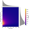 |
Fig. 2 Distribution of flux and half light radius for the simulated galaxies. |
4 Simulated datasets
4.1 Population model
We use the SFG-wide catalog from the Tiered Radio Extragalactic Continuum Simulation (T-RECS) (Bonaldi et al. 2018) for our population model. The relevant parameters from the T-RECS catalog used for galaxy simulation are: flux density I0 at frequency ν = 1.4 GHz, size, ellipticity, and position in the sky. We only consider galaxies in the flux range 50 μJy I0 < 200 μJy for this work. Using a flux cut ensures that all images have similar dynamic ranges while also excluding very bright sources which are not the primary target for weak-lensing studies. Similar flux cuts have been used in contemporary works (Harrison et al. 2020; Rivi et al. 2019; Patel et al. 2010). Figure 2 shows the distribution of flux and half light radius for the simulated galaxies. The training and testing sets are sampled from this distribution.
We assume that all galaxies have a Sérsic brightness profile:
![I(r) = I_e~ \text{exp} ~\left\{-b_{n_s}\left[\left(\frac{r}{r_e}\right)^{1/n_s}-1\right]\right\},](/articles/aa/full_html/2025/04/aa54072-25/aa54072-25-eq52.png) (24)
(24)
where Ie is the flux density at effective radius re, the Sérsic index (Sérsic 1963) ns parametrizes the curvature of the light profile, and bns is a scaling factor that depends on ns. We draw ns from the distribution  . This was done to minimize model-dependent biases. RadioLensfit assumes ns = 1.
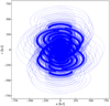 |
Fig. 3 Visibility coverage for a pointing at declination of δ = 30°. u and v are plotted in 1000 wavelength units kλ. |
4.2 Interferometer model
We then calculate the observed visibilities from these simulated sources based on the SKA-MID AA4 array configuration, which consists of 133 15-meter SKA-MID dishes and 64 13.5-meter MeerKAT dishes. We use this configuration since it is expected to provide the sensitivity and spatial resolution necessary to detect the shapes of high-redshift SFGs required for weak-lensing studies (Patel et al. 2014). We assume that all observations are made in a single frequency channel with a central frequency of ν0 = 1.4 GHz and a fractional bandwidth of △ν = 0.3ν0. Observations are carried out for 8-hour periods, from an hour angle (HA) of –4 hours to +4 hours, with visibilities sampled every 300 seconds, resulting in 1 853 376 individual positions.
A typical radio survey maps the sky using several pointings, each pointing covering a field of view containing multiple galaxies (Thompson et al. 2017). As a result, different galaxies have different effective PSF depending on the pointing direction and the relative galaxy position with respect to it. We partially emulated this variable PSF effect by changing the pointing direction to align with the center of the galaxy for each observation. This results in a variety of PSF shapes depending on the galaxy position on the sky. However, this does not account for the variation of PSF within a field of view. We aim to address this issue in a future work. Figure 3 illustrates the visibility coverage (uv coverage) for a pointing at declination of δ = 30°.
To simulate realistic observation conditions, uncorrelated Gaussian noise is added to each visibility. The root mean square (RMS) noise for the visibilities σV is computed based on the array sensitivity and observational parameters using the following relation (Thompson et al. 2017):
 (25)
(25)
where kB is the Boltzmann’s constant, Tsys is the system temperature, ηS is the antenna efficiency, Aeff is the effective dish area and τint is the integration time. For simplicity, we assume the same noise variance across all dishes, calculated using the parameters of the SKA-MID dishes. All the necessary parameters have been taken from Braun et al. (2019). Based on these assumptions, the RMS visibility noise is estimated to be σV ≈ 0.5 mJy. We do not investigate the effect of time/frequency smearing or phase calibration errors in this work. Visibility simulations were carried out using the Radio Astronomy Simulation, Calibration, and Imaging Library (RASCIL) package1.
4.3 Imaging settings
All images are simulated on a Npix = 128 128 pixel grid using the GalSim galaxy image simulation package (Rowe et al. 2015). This grid size is chosen to enhance computational efficiency while preserving the image quality. The intensity of each pixel is scaled such that the total flux in each galaxy image is equal to I0. The pixel scale θpix is calculated as θpix = λ0/(ΓDmax) where Γ is the oversampling factor, Dmax is the maximum baseline distance, and λ0 is the wavelength corresponding to the central frequency ν0 = 1.4 GHz. We selected Γ = 2 which makes the deconvolution tractable while maintaining a manageable computational cost. This results in a pixel scale of θpix = 0.143″.
During imaging, visibilities can be weighted in different ways to alter the natural response function of the instrument. Data weighting is essential to enhance the dynamic range of the image and adjust the synthesized beam to make the deconvolution more tractable (CASA Team 2022). We use Briggs or robust weighting scheme which creates a PSF that smoothly varies between natural and uniform weighting based on a tunable robustness parameter R (Briggs 1995). After evaluating various values of R, we selected R = 0.5 as an optimal balance between resolution and sensitivity. A detailed discussion on this choice is provided in Appendix B. With this configuration, the RMS pixel noise in the image domain is σ ≈ 0.71 μJy.
To facilitate training and evaluate the noise dependence of our methods, we applied quality cuts to the simulated dirty images. Specifically, we used the peak signal-to-noise ratio (peak S/N) statistic, defined as the ratio of peak intensity in a noise-free dirty image  to the RMS pixel noise σ:
 (26)
(26)
where σ is estimated from the edge pixels of the dirty image iD.
5 Experiments
5.1 Test dataset
We evaluate the performance of our framework using a simulated test set comprising 20 000 galaxies. The galaxies in the test set have varying sizes, fluxes, shapes, and PSFs. The PSFs are varied by changing the pointing center to the position of each galaxy. This is an important part of the analysis since it reflects the expected scenario in typical radio surveys, where each galaxy is associated with a unique PSF. This test set is referred to as the TS0 set. The TS0 set contains galaxies with an average peak S/N of ~24, and ~99% of galaxies have a peak S/N ≥ 3. The TS0 set is used to assess both the reconstruction quality and the shape measurement accuracy from different methods. Additionally, we created a smaller test set, referred to as the TSS set, by randomly sampling 2500 galaxies from the TS0 set. The TSS set is used to evaluate the RadioLensfit method to avoid long computation times.
For shear measurements, we utilized a separate simulated test set consisting of 1 million galaxies, hereafter referred to as the TS1 set. The TS1 set is divided into 100 shear fields, each containing 10 000 galaxies. The shear fields are sampled from a uniform distribution  , where α corresponds to the two shear components. The galaxies within a field have varying fluxes, sizes, and shapes but share the same PSF. To reduce shape noise, we simulate galaxies in 90° rotated pairs. This ensures that the average of galaxy ellipticities for a field is zero, thus eliminating any shape noise. For simplicity, all galaxy ensembles are generated with identical distributions of flux, size, and shape, differing only in the applied shear and PSF.
5.2 Training details
We use three neural networks in our work: the CNN denoiser, DRUNet; the PSF autoencoder; and the measurement network.
5.2.1 DRUNet
The DRUNet model is built and initialized using pre-trained weights provided by the DeepInverse library (Tachella et al. 2023). These weights are subsequently fine-tuned on a training set comprising 250 000 galaxy image pairs, each consisting of a noiseless and a corresponding noisy image. The training set contains galaxies with varying flux, size, and shape. Noisy images are simulated by adding Gaussian noise with varying noise levels. The network is trained using an ℓ1 loss function, consistent with the approach presented in the original work (Zhang et al. 2020).
Hyperparameter setting: The HQS-PnP algorithm includes four hyperparameters: the number of iterations K, the regularization weight λ, and the penalty terms at the first and last iterations (μk=0 and μk=K). Following Zhang et al. (2020), the penalty term μk is monotonically increased at each iteration following a logarithmic scale. These hyperparameters significantly impact the stability and accuracy of the image reconstruction process and require careful tuning for different datasets to achieve optimal performance. To efficiently search the hyperparameter space, we use the OPTUNA library (Akiba et al. 2019), which leverages Bayesian optimization techniques to find the optimal hyperparameters by minimizing the loss on a validation set.
Specifically, we use the Tree-structured Parzen estimator (Bergstra et al. 2011) to iteratively evaluate different hyperparameter configurations and minimize the total ℓ2 loss on a validation set containing 1000 galaxies. We employed an iterative strategy to define the hyperparameter search space, initially considering all positive numbers for each hyperparameter and progressively narrowing the range based on observed performance until it was sufficiently constrained for optimal tuning. Through this process, we determine the optimal hyperparameters as K = 30, λ = 2.49, μ0 = 10.86/σ2, and μK = 301.36/σ2.
We also assess the importance of hyperparameters using the fANOVA importance evaluator (Hutter et al. 2014) (as implemented in OPTUNA) and find that μK and λ have the greatest impact on the algorithm. This is expected, as they directly control the trade-off between the data fidelity term and the maximum regularization strength. We also observe an improvement in reconstruction quality when increasing the number of iterations (i.e., when K > 30), however, the improvement is not substantial enough to justify the increased computational costs. We direct the reader to Hurault et al. (2024) for the theoretical convergence of PnP algorithms.
5.2.2 Autoencoder
The autoencoder is trained using a training set of 100 000 PSFs. Different PSFs are calculated by varying the position of the pointing angle. We set the robustness parameter to R = −0.5 for the whole training set.
We tested a few network architecture choices, such as using deeper networks and variational autoencoders (Kingma & Welling 2019). However, we did not observe an improvement in the shape measurement after incorporating these modifications.
5.2.3 Measurement network
We follow a two-stage procedure to train the measurement network. In the first stage, the network is pre-trained using a training set of 250 000 true noiseless galaxy images. In the second stage, the network is fine-tuned using a training set of 250 000 reconstructed galaxy image-PSF pairs. This two-step approach is motivated by the expectation that pre-training on “simpler” data facilitates faster convergence during fine-tuning (Tripathi et al. 2024). The galaxies in the training sets have varying flux, size, shape, and position in the sky. The reconstructed galaxy images in the training set are generated using the HQS-PnP algorithm. To ensure robust training, a quality threshold of peak S/N ≥ 3 (as defined in Eq. (26)) is applied to the dirty images that are used to create the training set. This removes extremely noisy galaxies that could otherwise bias the training process.
We adopt an 80–20 training-validation split for all network training. The learning rate (LR) is initially set to 10−3 and gradually reduced by an order of magnitude when the validation loss has stopped decreasing, with a minimum LR of 10−6. We perform parameter optimization using the ADAM optimizer (Kingma & Ba 2015).
We optimize a few hyperparameters of the architecture, including the number of layers, the size of convolutional kernels and dense layers, the batch size, and the choice of optimizer using a random search strategy on a small manually chosen hyperparameter space. We do not perform an extensive hyperparameter tuning owing to the high training costs.
5.3 Implementation
DeepShape is built using the Python library PyTorch (Paszke et al. 2019). Our implementation and results, as well as instructions on how to use our code, are available in our online repository2.
We used the RASCIL implementation of MS-CLEAN. We used a maximum of 1000 iterations per deconvolution, with a CLEAN threshold of 1.2 × 10⁻⁸, a CLEAN fractional threshold of 3 × 10⁻⁵, and CLEAN scales of [0, 2, 4]. Although these parameters are conservative, we found that they are necessary to reconstruct the small and faint galaxies, with larger CLEAN scales or higher thresholds leading to significantly poorer quality images. In principle, the overall reconstruction quality can be improved by optimizing the parameters individually for each galaxy. However, this is a computationally intensive process, given the large number of galaxies and wide distribution of galaxy properties. We also use a maximum of 1000 CLEAN iterations to ensure that CLEAN and HQS-PnP have similar runtimes.
We implement RadioLensfit using the publicly available software from Rivi & Miller (2022). We run the code in the OpenMP mode to exploit all the available cores on a node and hence ensure computational efficiency. We modify several prior parameters in the default_params.h file to align with our datasets. Specifically, we set the System Equivalent Flux Density (SEFD) of SKA to SEFD_SKA = 263 Jy; define the scale length range from RMIN = 0.01 to RMAX = 4.08; and adjust the parameters for the source scale length-flux relation to ADD = 1.95, ESP = 0.51 and R_STD = 0.569.
As no publicly available library for implementing the SuperCALS method was found, we developed our own version, which is also available in our online repository. We have aimed to remain as faithful as possible to the original approach described in Harrison et al. (2020), with a few modifications. First, we use GalSim for shape estimation rather than Im3Shape method (Zuntz et al. 2013), to ensure faster computation time. Second, the ellipticity of the model sources is chosen to be ϵα = {0, ±0.1375, ±0.275, ±0.4125, ±0.55} as our datasets do not include galaxies with very high ellipticities.
6 Results
In this section, we present the results obtained using our framework. First, we evaluate the image reconstructions for the TS0 dataset, comparing the performance of the HQS-PnP method with that of MS-CLEAN. Next, we compare the shape measurement results derived from DeepShape, RadioLensfit, and SuperCALS. Finally, we report the shear measurement results for the TS1 dataset, using shape measurements performed by DeepShape.
6.1 Image reconstruction
We evaluate the performance of the HQS-PnP algorithm against the MS-CLEAN method using the TS0 dataset. We use the normalized mean square error (NMSE) metric to assess and compare the reconstruction quality from the two methods:
 (27)
(27)
where  and
and  are the p-th reconstructed and true images, respectively, within a set containing P images and ||.||2 corresponds to the ℓ2 norm. We find that the reconstruction quality for both methods exhibits a strong dependence on the peak S/N of the dirty images. Figure 4 illustrates the variation of NMSE as a function of peak S/N for the two methods. As shown in the plot, the NMSE is highest in the lowest-peak S/N bin and decreases progressively with increasing peak S/N for both methods. This result is expected as most reconstruction methods work better for brighter, less noisy objects, and the peak S/N of a dirty image is directly related to these quantities. The HQS-PnP algorithm outperforms MS-CLEAN across all peak S/N levels in terms of NMSE. The performance difference is particularly prominent for the lowest peak S/N objects and gradually decreases with increasing S/N. The superior performance of HQS-PnP in the low peak S/N regime is likely due to its advanced regularization capabilities.
Figure 5 illustrates the reconstructed images from both methods for a random subset of galaxies from the TS0 set. The images reconstructed from the HQS-PnP method have a lower total flux compared to the ground truth. This is likely due to the regularization process, which reduces the sharpness of the image. This could be improved by using an additional scaling factor; however, such a correction is not critical for shape measurements.
The residual images (as defined in Eq. (5)) from the two methods are illustrated in Fig. 6. We find that the residual images from the HQS-PnP reconstructions resemble pure noise, and further deconvolution of these residuals does not provide any additional information. This is a promising outcome; however, our analysis is limited to galaxies at the pointing center, where the w-term effects are minimal. In real observational scenarios, multiple deconvolution cycles may be necessary. In contrast, the residuals from MS-CLEAN retain significant structural information. These residuals can be deconvolved again for a better estimate. However, such a process is computationally expensive due to the complexity of gridding/de-gridding operators.
We also compare the two methods in terms of shape retention in the reconstructed images. To do so, we first measure galaxy shapes from the reconstructed images using GalSim (standard moment-based method). We then calculate the root mean square error (RMSE) of ellipticity measurements as:
 (28)
(28)
where α ∈ (1, 2);  is the true ellipticity;
  is the ellipticity measured from the reconstructed images and ⟨.⟩ denotes the average over a test set. For reference, we also calculate the RMSE for shape measurements obtained directly from the dirty images. We detail the RMSE for shape measurements from the three types of images in Table 1.
Our results show that shape measurements from the HQSPnP reconstructions exhibit the lowest RMSE, followed by MS-CLEAN reconstructions, with dirty images performing the worst. Dirty images are significantly affected by PSF smearing and pixel noise, leading to unreliable shape measurements, as reflected in their high RMSE. While MS-CLEAN partially recovers some of the lost shape information, it still lags behind HQS-PnP. These results emphasize the importance of advanced image reconstruction techniques, such as the HQS-PnP method, to maximize shape information recovery, particularly in the low peak S/N regime.
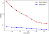 |
Fig. 4 Normalized mean square error, NMSE, as a function of peak S/N bin for the TS0 set. The last bin contains all dirty images with peak S/N > 50. |
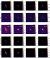 |
Fig. 5 Examples of four simulated galaxies and associated PSFs from the TS0 set. From top to bottom, the panels show the ground truth image, PSF, dirty image, and reconstructed images using MS-CLEAN and HQS-PnP, respectively. The top right corner of the dirty images shows the peak S/N. |
RMSE for shape measurements from different images using GalSim.
Comparison metrics for the ellipticity measurements from different methods.
6.2 Shape measurement
We evaluate the performance of the DeepShape in comparison to the SuperCALS and RadioLensfit methods using the TS0 and TSS datasets. To assess the accuracy of ellipticity measurements, we compute the root mean square error (RMSE) as defined in Eq. (28) for each method. Additionally, we calculate the Pearson correlation coefficient ρα for each ellipticity component:
 (29)
(29)
where  is the covariance between the predicted ellipticities and the ground truth and
  and
and  are the respective standard deviations. The Pearson correlation coefficient ρα quantifies the dispersion of shape measurements from a method. Ideally, a shape measurement method should yield a ρα value close to 1.
To further characterize the performance, we calculate the linear shape measurement bias: a multiplicative factor  and an additive factor
  . These are estimated by calculating the slope and the intercept of the best-fit linear relation between the ground truth
  and the measurement residual
  . A summary of the comparison metrics for the two ellipticity components is presented in Table 2. The residuals for the first ellipticity component are shown in Fig. 7.
We find that the SuperCALS method performs notably worse than the other two methods. This is likely due to its reliance on MS-CLEAN, which does not yield optimal reconstructions in the low-flux regime probed in this study (as demonstrated in Sect. 6.1). The performance of SuperCALS could potentially be improved by replacing MS-CLEAN with a more advanced reconstruction algorithm, such as the HQS-PnP method. In contrast, RadioLensfit and DeepShape show comparable performance across several evaluation metrics, with RadioLensfit slightly outperforming DeepShape in most cases (except for  ). However, RadioLensfit fails to resolve approximately 27% of galaxies in the TSS set due to noisy likelihoods. This may be attributed to the assumption of an exponential brightness profile in RadioLensfit, whereas our test set consists of galaxies with Sérsic profiles of different indices. As a result, we restrict our comparison to the subset of galaxies in the TSS set that were resolved by RadioLensfit, which we refer to as the TSS* set.
The average flux of the TSS* set is approximately 20% lower than that of the TS0 set. Consequently, DeepShape’s predictions for the TSS* set are slightly less accurate compared to the TS0 set, as reflected in the evaluation metrics. For the TS0 set, DeepShape achieves a multiplicative shape measurement bias on the order of a few 10−3 and an additive bias on the order of a few 10−4. These bias levels meet the measurement requirements set for next-generation weak-lensing experiments, such as Euclid (Jansen et al. 2024) and SKA-MID (Patel et al. 2015). A detailed comparison of the computational costs for these methods is presented in Sect. 6.2.2.
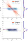 |
Fig. 7 Shape measurement residuals from different methods as a function of input ellipticity (for the first ellipticity component ϵ1). The 2D contours are calculated using a kernel density estimation. The colored dashed lines show the best-fit linear relations for the methods. The right panels show the marginal 1D distribution of the residuals. Top: measurement residuals from DeepShape and SuperCALS on TS0 set; bottom: measurement residuals from DeepShape and RadioLensfit on TSS* set. |
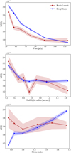 |
Fig. 8 Mean square error of ϵ1 measurements, MSE1, as a function of galaxy bins. From top to bottom, galaxies are binned based on flux, half-light radius, and Sérsic index, respectively. The shaded region corresponds to the error on the MSE computed using the variance of a chi-squared random variable. |
6.2.1 Dependence on galaxy properties
In this section, we analyze how the accuracy of DeepShape and RadioLensfit predictions varies with different galaxy properties. This is done by binning galaxies according to different properties and calculating the mean square error (MSE) for ellipticity predictions within each bin. For DeepShape, MSE calculations are performed using the TS0 set, while for RadioLensfit, we use the TSS* set. The MSE corresponds to the square of the RMSE, as defined in Eq. (28). Additionally, we estimate the error bars on the MSE using the variance of a chi-squared random variable. The results are presented in Fig. 8. The SuperCALS method is excluded from this comparison due to its significantly poorer performance relative to the other two methods.
Our results indicate a strong inverse correlation between MSE and both galaxy flux and half-light radius for both methods, with better performance observed for brighter and larger galaxies. This is expected, as these galaxies typically have more pixels above the noise threshold, allowing for more accurate shape constraints. Similar dependencies on flux and size have been extensively studied in the optical domain (Kaiser et al. 1995; Massey et al. 2007; Mandelbaum et al. 2014). Furthermore, we observe a correlation between MSE and the Sérsic index (ns), although the trend differs for DeepShape and RadioLensfit. For DeepShape, MSE increases with ns, likely because high-ns galaxies exhibit a steeper flux decline away from their centers, concentrating most of the flux in the central pixels. As a result, outer pixels are more susceptible to being masked by noise, leading to less accurate shape estimates. Further discussion on this effect is provided in Appendix A. In contrast, RadioLensfit is unaffected by this issue, since it operates in the visibility domain. However, its performance is highest around ns = 1, as expected, given its assumption of exponential profiles.
We also expect a correlation between the MSE and the peak S/N of the galaxy, though this relationship is not as straight-forward. The peak S/N of a galaxy is influenced by the total flux, the size, and the Sérsic index of the galaxy. For instance, a high peak S/N does not always indicate improved shape measurement since galaxies with a small size or a high Sérsic index can also have a high peak S/N while still resulting in less accurate shape estimates. Therefore, it is more fundamental to analyze the dependence of the MSE on the flux, size, and Sérsic index.
Overall, both methods produce MSE values within a comparable range across different galaxy bins. However, the error bars on the MSE for RadioLensfit predictions are larger, mainly due to the smaller size of the TSS* set relative to the TSS set. The reduced test set size for RadioLensfit is a result of both its slower computation time and its inability to resolve approximately 27% of galaxies due to a noisy likelihood.
6.2.2 Computational costs
DeepShape can be compiled using GPUs or CPUs. In particular, we use a single Quadro RTX 6000 GPU for all the training/testing associated with DeepShape. The primary computational cost of our method arises from the initial training of the networks. Training the autoencoder requires approximately 8 hours. For the DRUNet denoiser, we leverage pre-trained weights and perform fine-tuning, which significantly reduces training time to around 100 hours. The two-stage training of the measurement network takes approximately 300 hours. As with most deep learning models, once the networks are trained, the subsequent predictions are much faster.
The HQS-PnP algorithm reconstructs a galaxy image in approximately 120 milliseconds, which is comparable to the runtime of a standard MS-CLEAN reconstruction. The measurement network requires about 100 milliseconds to predict ellipticity from a reconstructed image-PSF pair. Overall, DeepShape takes approximately 220 milliseconds to predict the shape from a given dirty image-PSF pair.
We implemented the SuperCALS and RadioLensfit methods on a single node equipped with an AMD EPYC 7313 CPU with 252GB of primary memory. The SuperCALS method is slightly faster than DeepShape, taking approximately 180 milliseconds to generate a calibrated shape estimate from a dirty image/PSF pair. In contrast, RadioLensfit is considerably slower, requiring around 4 minutes to predict the shape from a given visibility table.
The execution times of all these methods can be further optimized by leveraging a distributed system, such as a High-Performance Computing (HPC) cluster. This would be particularly beneficial for handling larger datasets. Rivi & Miller (2022) proposed an MPI-based version of the RadioLensfit code, enabling the simultaneous shape estimation of multiple galaxies within the field of view, thereby enhancing computational efficiency.
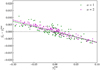 |
Fig. 9 Shear measurement residuals as a function of input shear. Each point represents the average of 10 000 shape measurements from DeepShape. The two colors indicate the two shear components, as indicated in the legend. The colored dashed lines indicate the best-fit linear relation for the two components. |
6.3 Shear measurement
We measure the shear  for each field of the TS1 set by calculating the average of the DeepShape shape predictions:
  where
where  are the DeepShape predictions. We estimate the shear bias
  and
and  by taking the best-fit linear relation between the shear measurement residual
  and the input shear
  . We plot the shear measurement residuals for the TS1 set in Fig. 9. The estimated shear bias factors for the two shear components are:
 (30)
(30)
The results indicate different bias values for the two shear components, which can be attributed to the asymmetry in visibility coverage. We estimate an additive bias that is within the SKAMID requirements (|Cα| < 8.2 10−4). The main source of additive bias is leakage due to anisotropic sampling of the uv-space or anisotropy of the PSF. The TS1 set contains galaxies with different PSFs, which exhibit different levels of anisotropy. The low additive bias observed indicates that our method effectively mitigates the effects of arbitrary PSFs. However, the estimated multiplicative bias factor is higher than the requirements for SKA-MID (|Mα| < 6.7 10−3) by an order of magnitude. The higher shear bias does not inherently reflect the limitations of DeepShape but rather a limitation of the shear estimator used. This is evident from the fact that the estimated shear bias,  , is significantly larger than the estimated shape measurement bias,
  .
.
Existing optical weak-lensing surveys also report shear biases that exceed their cosmological requirements, necessitating a calibration step to mitigate these biases (Refregier et al. 2012; Heymans et al. 2012). A common approach involves computing a weighted average of galaxies, with weights assigned based on their properties such as S/N, flux, ellipticity, size, etc. (Bernstein & Armstrong 2014; Fenech Conti et al. 2017). In our analysis, we explored a similar strategy by applying different quality cuts to the galaxy ensemble. This can be interpreted as an extreme weighting scheme, where galaxies are either fully included (weight = 1) or excluded (weight = 0). We find that the estimated shear bias improves when applying a minimum flux threshold or a maximum ellipticity |ϵtrue| threshold on the galaxy ensemble. This dependence of  on these cuts is plotted in Fig. 10. A similar enhancement in shear bias for radio galaxies was also observed when flux/ellipticity cuts were applied in Rivi et al. (2016). However, we find no improvement in the estimated bias when using cuts based on size or Sérsic index. In principle, multiple quality cuts could be combined to create a “gold” sample for precise shear measurements (Patel et al. 2010).
For additive bias  , we do not observe a strong correlation with any specific ensemble property, and it remains within acceptable limits across all tested cuts. However, it is important to note that applying quality cuts reduces the size of the galaxy ensemble, which increases the uncertainty in the estimated bias parameters.
These findings highlight the strong dependence of shear estimation on the distribution of galaxy properties, such as source ellipticity and flux. Therefore, an ideal shear estimator should account for the properties of the galaxy population. Incorporating an optimized weighting scheme or quality cuts could further enhance shear estimates to achieve the required accuracy. Recent studies have also explored deep learning-based networks that incorporate galaxy properties such as flux, size, and measured ellipticity to obtain a calibrated shear estimate (Tewes et al. 2019; Zhang et al. 2024). However, the development of a precise shear estimator is a much broader topic and falls beyond the scope of this work.
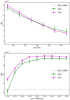 |
Fig. 10 Estimated multiplicative shear bias as a function of quality cuts on galaxy ensemble. The dotted black line shows the SKA-MID bias requirements for comparison. Top: quality cut based on minimum flux, bottom: quality cut based on maximum ellipticity. |
7 Conclusions and future work
7.1 Conclusions
In this work, we presented a fully automated supervised deep learning framework, DeepShape, designed to recover galaxy shapes from dirty image-PSF pairs of isolated radio galaxies. DeepShape consists of two modules. The first module is an image reconstruction algorithm that reconstructs images of isolated radio galaxies. The second module is a measurement network that predicts galaxy shapes based on the reconstructed image and the associated PSF.
To evaluate our framework, we developed a simulation pipeline that generates galaxy datasets based on the SKAMID AA4 array configuration and the TRECS galaxy catalog (Bonaldi et al. 2018) for faint star-forming radio galaxies. We compare our reconstruction method against the standard MSCLEAN reconstruction algorithm. We found that our method yields significantly improved image reconstructions than MSCLEAN in terms of normalized mean square error, shape measurement error, and image residuals. Notably, the performance gap between the two methods becomes more pronounced at lower peak S/N values.
For radio shape measurement, we tested three methods: DeepShape (our proposed framework), RadioLensfit (Rivi et al. 2016), and SuperCALS (Harrison et al. 2020). Our method achieves comparable measurement accuracy at much faster computational times compared to RadioLensfit and much higher measurement accuracy at comparable computational times compared to SuperCALS. This makes our framework an optimal choice for processing the large data volumes anticipated from upcoming radio weak-lensing surveys. Another key strength of our framework is the ability to deal with variable PSFs. This allows us to make shape predictions for different pointings without needing to retrain the network for each pointing, enabling us to effectively leverage the large sky coverage of upcoming weak-lensing surveys.
We also used our framework for shear estimation and successfully recovered shear estimates on simulated datasets with an additive bias that meets the SKA-MID requirements. Although our method exhibits a significant multiplicative bias, this is likely a limitation of the shear estimator used rather than the shape measurements from DeepShape. We show how this can be improved by using weights or quality cuts based on galaxy properties.
7.2 Future work
There are several potential avenues for extending our work. A key next step is to evaluate the compatibility of different shear calibration methods with our framework. Possible approaches include employing a weighted shear estimator (Bernstein & Armstrong 2014; Fenech Conti et al. 2017), applying empirical bias corrections using parameters derived from simulations (Kacprzak et al. 2012; Harrison et al. 2020), or utilizing deep learning models for shear calibration (Tewes et al. 2019; Zhang et al. 2024).
Another potential extension is to adapt our framework for scenarios where individual galaxies are randomly distributed across the field of view rather than being centered at the phase center. Although we do test the variation of PSF due to a change in pointing direction, we do not address the issue of PSF variation within a field of view. Additionally, we aim to incorporate smearing and direction-dependent effects into our simulation pipeline, as these factors may impact the reconstruction quality of the HQS-PnP method and help determine whether additional major loop iterations are required.
We also seek to address the challenge of source separation. Since galaxies are not localized in the visibility domain, isolating individual sources is a complex task. To tackle this, we would likely need to use an initial source separation step to extract individual sources from larger fields. This could be achieved in the visibility domain using a phase shift and gridding technique similar to that proposed in Rivi & Miller (2018) or through source separation methods in the image domain (Melchior et al. 2018; Burke et al. 2019; Merz et al. 2023).
Lastly, we plan to enhance the realism of our test set by incorporating galaxies with complex structures, such as bulges, disks, and knots. Additionally, we plan to extend our analysis to low-peak S/N galaxies, either by including fainter sources or by evaluating performance under higher noise levels.
Acknowledgements
This research was funded by the Agence Nationale de la Recherche (ANR) under the project ANR-22-CE31-0014-01 TOSCA. The authors thank Marzia Rivi and Ian Harrison for useful discussions.
Appendix A Effect of Sérsic index
As illustrated in Fig. 8, DeepShape’s prediction accuracy declines sharply with increasing Sérsic index (ns). Galaxies with higher ns concentrate a greater fraction of their flux near the center compared to lower ns galaxies, even when their half-light radii are the same. Consequently, the number of pixels above a given noise threshold is lower for high-ns galaxies. This trend is illustrated in Fig. A.1, which shows how the number of pixels above the noise threshold varies with ns. Specifically, at low and high noise levels, the effective number of pixels remains independent of ns. However, at intermediate noise levels, high-ns galaxies have fewer effective pixels compared to low-ns galaxies. As a result, shape information is carried by a reduced number of pixels, leading to less accurate shape estimates.
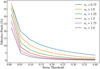 |
Fig. A.1 Effective number of pixels as a function of noise threshold. The different curves correspond to a galaxy with fixed flux, shape, and size but varying ns. The noise threshold is calculated with respect to the peak flux of the galaxy. |
To further examine this effect, we evaluate the RMSE of DeepShape’s shape measurements for true galaxies at different noise levels. Here, “true galaxies” refers to galaxies without any PSF effects, ensuring that any errors stem solely from limitations in the shape measurement network rather than reconstruction artifacts. Figure A.2 shows the variation of RMSE with ns for different peak S/N regimes. In the absence of noise, RMSE remains largely uncorrelated with ns since all galaxy pixels contribute to the shape measurement. However, at peak S/N levels of 50 and 100, noise starts to obscure lower-flux pixels. Since galaxies with higher ns have a greater proportion of low-flux pixels, their shape estimates degrade more significantly. At even higher noise levels (peak S/N of 5 and 10), the RMSE becomes independent of ns because most galaxy pixels are already buried in noise, forcing shape information to be derived primarily from the central pixels, regardless of ns. We speculate that using higherresolution images could help mitigate this issue; however, further investigation is beyond the scope of this paper.
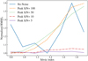 |
Fig. A.2 RMSE of DeepShape measurements for first ellipticity component as a function of Sérsic index. The different curves correspond to different peak S/N regimes, as indicated by the legend. Each curve has been normalized using its minimum value to show only the relative variation of RMSE with ns. |
Appendix B Effect of robustness parameter
Briggs weighting depends on tunable parameter R that defines the trade-off between sensitivity and resolution. In Briggs weighting, each visibility measurement Vi falling in the k-th grid cell is given an imaging weight wi such that:
 (B.1)
(B.1)
 (B.2)
(B.2)
where σi is the noise variance of the i-th visibility and  is the total noise variance in the k-th grid cell. A value of R = 2 is equivalent to natural weighting, meaning each visibility is assigned the same weight
  . This provides high sensitivity with respect to noise, however, the resulting PSF has extended sidelobes, which leads to poor resolution. A value of R = −2 is equivalent to uniform weighting, meaning each measured spatial frequency is assigned equal weight
  . This means that the longer baselines are up-weighted, which results in higher resolution. However, this weighting scheme has a very low noise sensitivity. The effect of R on the PSF and dirty images for different noise levels is illustrated in Fig. B.1. As shown, uniform weighting provides high-resolution images at low noise levels. However, the dirty images gradually lose more and more shape information with increasing noise levels. For natural weighting, the PSF has extensive side lobes, which causes the dirty image to be heavily smeared. This makes reconstruction difficult even at low noise levels. A value of R = - 0.5 provides an optimal middle ground between the two extreme cases.
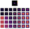 |
Fig. B.1 Example galaxy from the T-RECS catalog with I = 168 μJy and ϵtrue = (0.32, 0.16). The ground truth is plotted in Fig. B.1a. The top row of Fig. B.1b shows the associated PSFs. The second to the fourth row of Fig. B.1b show the dirty images for different noise levels (actual noise level mentioned in the legend) with noise increasing from top to bottom. σV corresponds to the expected visibility noise level calculated using Eq. 25. Different columns correspond to different values of R. |
References
- Akiba, T., Sano, S., Yanase, T., Ohta, T., & Koyama, M. 2019, in The 25th ACM SIGKDD International Conference on Knowledge Discovery & Data Mining, 2623 [CrossRef] [Google Scholar]
- Arras, P., Bester, H. L., Perley, R. A., et al. 2021, A&A, 646, A84 [NASA ADS] [CrossRef] [EDP Sciences] [Google Scholar]
- Bacon, D. J., Refregier, A. R., & Ellis, R. S. 2000, MNRAS, 318, 625 [NASA ADS] [CrossRef] [Google Scholar]
- Battye, R. A., Brown, M. L., Casey, C. M., et al. 2020, MNRAS, 495, 1706 [Google Scholar]
- Bengtsson Bernander, K., Sintorn, I.-M., Strand, R., & Nyström, I. 2024, NatSR, 14, 14995 [Google Scholar]
- Bergstra, J., Bardenet, R., Bengio, Y., & Kégl, B. 2011, in Algorithms for Hyper-Parameter Optimization in NeurIPS [Google Scholar]
- Bernstein, G. M., & Armstrong, R. 2014, MNRAS, 438, 1880 [NASA ADS] [CrossRef] [Google Scholar]
- Bonaldi, A., Bonato, M., Galluzzi, V., et al. 2018, MNRAS, 482, 2 [Google Scholar]
- Braun, R., Bonaldi, A., Bourke, T., Keane, E., & Wagg, J. 2019, arXiv e-prints [arXiv:1912.12699] [Google Scholar]
- Briggs, D. S. 1995, PhD thesis, New Mexico Institute of Mining and Technology [Google Scholar]
- Burke, C. J., Aleo, P. D., Chen, Y.-C., et al. 2019, MNRAS, 490, 3952 [NASA ADS] [CrossRef] [Google Scholar]
- CASA Team, Bean, B., Bhatnagar, S., et al. 2022, PASP, 134, 114501 [NASA ADS] [CrossRef] [Google Scholar]
- Cesa, G., Lang, L., & Weiler, M. 2022, in A Program to Build E(N)-Equivariant Steerable CNNs in ICLR [Google Scholar]
- Chang, T., Refregier, A., & Helfand, D. J. 2004, ApJ, 617, 794 [Google Scholar]
- Chidester, B., Zhou, T., Do, M. N., & Ma, J. 2019, Bioinformatics, 35, 1530 [Google Scholar]
- Cohen, T., & Welling, M. 2016, in ICML, 2990 [Google Scholar]
- Cornwell, T. J. 2008, ISTSP, 2, 793 [Google Scholar]
- Fenech Conti, I., Herbonnet, R., Hoekstra, H., et al. 2017, MNRAS, 467, 1627 [NASA ADS] [Google Scholar]
- Goodfellow, I., Bengio, Y., & Courville, A. 2016, Deep Learning (MIT Press) [Google Scholar]
- Harrison, I., Brown, M. L., Tunbridge, B., et al. 2020, MNRAS, 495, 1737 [Google Scholar]
- Heymans, C., Van Waerbeke, L., Bacon, D., et al. 2006, MNRAS, 368, 1323 [Google Scholar]
- Heymans, C., Van Waerbeke, L., Miller, L., et al. 2012, MNRAS, 427, 146 [Google Scholar]
- Högbom, J. A. 1974, A&AS, 15, 417 [Google Scholar]
- Hurault, S., Chambolle, A., Leclaire, A., & Papadakis, N. 2024, JMIV, 66, 616 [Google Scholar]
- Huterer, D., Takada, M., Bernstein, G., & Jain, B. 2006, MNRAS, 366, 101 [Google Scholar]
- Hutter, F., Hoos, H., & Leyton-Brown, K. 2014, in ICML, 754 [Google Scholar]
- Jansen, H., Tewes, M., Schrabback, T., et al. 2024, A&A, 683, A240 [NASA ADS] [CrossRef] [EDP Sciences] [Google Scholar]
- Kacprzak, T., Zuntz, J., Rowe, B., et al. 2012, MNRAS, 427, 2711 [Google Scholar]
- Kaiser, N., Squires, G., & Broadhurst, T. 1995, ApJ, 449, 460 [Google Scholar]
- Kilbinger, M. 2015, RPPh, 78, 086901 [Google Scholar]
- Kingma, D. P., & Ba, J. 2015, in Adam: A Method for Stochastic Optimization in ICLR [Google Scholar]
- Kingma, D. P., & Welling, M. 2019, Found. Trends Mach. Learn., 12, 307 [Google Scholar]
- Lafarge, M. W., Bekkers, E. J., Pluim, J. P. W., Duits, R., & Veta, M. 2020, Med. Image Anal., 68, 101849 [Google Scholar]
- Lines, N. E. P., Font-Quer Roset, J., & Scaife, A. M. M. 2024, RASTI, 3, 347 [Google Scholar]
- Liu, J., Asif, M. S., Wohlberg, B., & Kamilov, U. S. 2021, in NeurIPS, 453, 13 [Google Scholar]
- Mandelbaum, R., Rowe, B., Bosch, J., et al. 2014, ApJS, 212, 5 [Google Scholar]
- Massey, R., Heymans, C., Bergé, J., et al. 2007, MNRAS, 376, 13 [Google Scholar]
- Massey, R., Hoekstra, H., Kitching, T., et al. 2013, MNRAS, 429, 661 [Google Scholar]
- Melchior, P., Moolekamp, F., Jerdee, M., et al. 2018, A&C, 24, 129 [Google Scholar]
- Merz, G., Liu, Y., Burke, C. J., et al. 2023, MNRAS, 526, 1122 [NASA ADS] [CrossRef] [Google Scholar]
- Müller, H., & Lobanov, A. P. 2023, A&A, 672, A26 [NASA ADS] [CrossRef] [EDP Sciences] [Google Scholar]
- Nikolova, M., & Ng, M. K. P. 2005, SJSC, 27, 937 [Google Scholar]
- Ongie, G., Jalal, A., Metzler, C. A., et al. 2020, IEEE J. Sel. Areas Inform.Therory, 1, 39 [Google Scholar]
- Pandya, S., Patel, P. O. F., & Blazek, J. 2023, arXiv e-prints [arXiv:2311.01500] [Google Scholar]
- Parikh, N., & Boyd, S. 2014, Proximal Algorithms (Now Foundations and Trends) [CrossRef] [Google Scholar]
- Paszke, A., Gross, S., Massa, F., et al. 2019, in NeurIPS, 721, 12 [Google Scholar]
- Patel, P., Bacon, D. J., Beswick, R. J., Muxlow, T. W. B., & Hoyle, B. 2010, MNRAS, 401, 2572 [Google Scholar]
- Patel, P., Abdalla, F. B., Bacon, D. J., et al. 2014, MNRAS, 444, 2893 [Google Scholar]
- Patel, P., Harrison, I., Makhathini, S., et al. 2015, in Advancing Astrophysics with the Square Kilometre Array (AASKA14), 30 [Google Scholar]
- Paulin-Henriksson, S., Amara, A., Voigt, L., Refregier, A., & Bridle, S. L. 2008, A&A, 484, 67 [NASA ADS] [CrossRef] [EDP Sciences] [Google Scholar]
- Paulin-Henriksson, S., Refregier, A., & Amara, A. 2009, A&A, 500, 647 [NASA ADS] [CrossRef] [EDP Sciences] [Google Scholar]
- Refregier, A., Kacprzak, T., Amara, A., Bridle, S., & Rowe, B. 2012, MNRAS, 425, 1951 [Google Scholar]
- Ribli, D., Dobos, L., & Csabai, I. 2019, MNRAS, 489, 4847 [NASA ADS] [CrossRef] [Google Scholar]
- Rivi, M., & Miller, L. 2018, MNRAS, 476, 2053 [Google Scholar]
- Rivi, M., & Miller, L. 2022, A&C, 39, 100574 [Google Scholar]
- Rivi, M., & Miller, L. 2022, RadioLensfit: Radio weak lensing shear measurement in the visibility domain, Astrophysics Source Code Library [record ascl:2208.019] [Google Scholar]
- Rivi, M., Miller, L., Makhathini, S., & Abdalla, F. B. 2016, MNRAS, 463, 1881 [Google Scholar]
- Rivi, M., Lochner, M., Balan, S. T., Harrison, I., & Abdalla, F. B. 2019, MNRAS, 482, 1096 [Google Scholar]
- Rodriguez Salas, R., Dokládal, P., & Dokladalova, E. 2021, J. Vis. Commun. Image Repr., 75, 103054 [Google Scholar]
- Ronneberger, O., Fischer, P., & Brox, T. 2015, in MICCAI, 234 [Google Scholar]
- Rowe, B. T., Jarvis, M., Mandelbaum, R., et al. 2015, A&C, 10, 121 [Google Scholar]
- Scaife, A. M. M., & Porter, F. 2021, MNRAS, 503, 2369 [CrossRef] [Google Scholar]
- Seitz, C., & Schneider, P. 1997, A&A, 318, 687 [NASA ADS] [Google Scholar]
- Sérsic, J. L. 1963, Bol. Asoc. Argentina Astron. Plata Argentina, 6, 41 [Google Scholar]
- Sheldon, E. S., & Huff, E. M. 2017, ApJ, 841, 24 [NASA ADS] [CrossRef] [Google Scholar]
- Sun, Y., Wohlberg, B., & Kamilov, U. S. 2019, IEEE Trans. Comp. Imaging, 5, 395 [Google Scholar]
- Tachella, J., Chen, D., Hurault, S., & Terris, M. 2023, DeepInverse: a Pytorch library for imaging with deep learning [Google Scholar]
- Terris, M., Dabbech, A., Tang, C., & Wiaux, Y. 2022, MNRAS, 518, 604 [NASA ADS] [CrossRef] [Google Scholar]
- Tewes, M., Kuntzer, T., Nakajima, R., et al. 2019, A&A, 621, A36 [NASA ADS] [CrossRef] [EDP Sciences] [Google Scholar]
- Thompson, A. R., Moran, J. M., & Swenson, George W., J. 2017, Interferometry and Synthesis in Radio Astronomy, 3rd edn. (Springer Open) [CrossRef] [Google Scholar]
- Tripathi, P., Wang, S., Prunet, S., & Ferrari, A. 2024, in EUSIPCO (IEEE), 2377 [Google Scholar]
- Tyson, J. A., Valdes, F., & Wenk, R. A. 1990, ApJ, 349, L1 [CrossRef] [Google Scholar]
- Vincent, P., Larochelle, H., Bengio, Y., & Manzagol, P.-A. 2008, in ICML [Google Scholar]
- Voigt, L. M., & Bridle, S. L. 2010, MNRAS, 404, 458 [Google Scholar]
- Weiler, M., & Cesa, G. 2019, in NeurIPS [Google Scholar]
- Weltman, A., Bull, P., Camera, S., et al. 2020, PASA, 37, e002 [Google Scholar]
- Wittman, D. M., Tyson, J. A., Kirkman, D., Dell’Antonio, I., & Bernstein, G. 2000, Nature, 405, 143 [NASA ADS] [CrossRef] [Google Scholar]
- Xu, X., Sun, Y., Liu, J., Wohlberg, B., & Kamilov, U. S. 2020, ISPL, 27, 1280 [Google Scholar]
- Zhang, J., Luo, W., & Foucaud, S. 2015, J. Cosmology Astropart. Phys., 2015, 024 [CrossRef] [Google Scholar]
- Zhang, K., Zuo, W., Chen, Y., Meng, D., & Zhang, L. 2017, ITIP, 26, 3142 [Google Scholar]
- Zhang, K., Li, Y., Zuo, W., et al. 2020, ITPAM, 44, 6360 [Google Scholar]
- Zhang, Z., Shan, H., Li, N., et al. 2024, A&A, 683, A209 [NASA ADS] [CrossRef] [EDP Sciences] [Google Scholar]
- Zuntz, J., Kacprzak, T., Voigt, L., et al. 2013, MNRAS, 434, 1604 [NASA ADS] [CrossRef] [Google Scholar]
All Tables
All Figures
|
Fig. 1 Architecture of the measurement network. The decoder block is shown just for reference and is not a part of the network. All layers have a ReLU activation except the final dense layer, which has a tanh activation. |
| In the text | |
|
Fig. 2 Distribution of flux and half light radius for the simulated galaxies. |
| In the text | |
|
Fig. 3 Visibility coverage for a pointing at declination of δ = 30°. u and v are plotted in 1000 wavelength units kλ. |
| In the text | |
|
Fig. 4 Normalized mean square error, NMSE, as a function of peak S/N bin for the TS0 set. The last bin contains all dirty images with peak S/N > 50. |
| In the text | |
|
Fig. 5 Examples of four simulated galaxies and associated PSFs from the TS0 set. From top to bottom, the panels show the ground truth image, PSF, dirty image, and reconstructed images using MS-CLEAN and HQS-PnP, respectively. The top right corner of the dirty images shows the peak S/N. |
| In the text | |
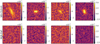 |
Fig. 6 Residual images from the two methods for the galaxies illustrated in Fig. 5. |
| In the text | |
|
Fig. 7 Shape measurement residuals from different methods as a function of input ellipticity (for the first ellipticity component ϵ1). The 2D contours are calculated using a kernel density estimation. The colored dashed lines show the best-fit linear relations for the methods. The right panels show the marginal 1D distribution of the residuals. Top: measurement residuals from DeepShape and SuperCALS on TS0 set; bottom: measurement residuals from DeepShape and RadioLensfit on TSS* set. |
| In the text | |
|
Fig. 8 Mean square error of ϵ1 measurements, MSE1, as a function of galaxy bins. From top to bottom, galaxies are binned based on flux, half-light radius, and Sérsic index, respectively. The shaded region corresponds to the error on the MSE computed using the variance of a chi-squared random variable. |
| In the text | |
|
Fig. 9 Shear measurement residuals as a function of input shear. Each point represents the average of 10 000 shape measurements from DeepShape. The two colors indicate the two shear components, as indicated in the legend. The colored dashed lines indicate the best-fit linear relation for the two components. |
| In the text | |
|
Fig. 10 Estimated multiplicative shear bias as a function of quality cuts on galaxy ensemble. The dotted black line shows the SKA-MID bias requirements for comparison. Top: quality cut based on minimum flux, bottom: quality cut based on maximum ellipticity. |
| In the text | |
|
Fig. A.1 Effective number of pixels as a function of noise threshold. The different curves correspond to a galaxy with fixed flux, shape, and size but varying ns. The noise threshold is calculated with respect to the peak flux of the galaxy. |
| In the text | |
|
Fig. A.2 RMSE of DeepShape measurements for first ellipticity component as a function of Sérsic index. The different curves correspond to different peak S/N regimes, as indicated by the legend. Each curve has been normalized using its minimum value to show only the relative variation of RMSE with ns. |
| In the text | |
|
Fig. B.1 Example galaxy from the T-RECS catalog with I = 168 μJy and ϵtrue = (0.32, 0.16). The ground truth is plotted in Fig. B.1a. The top row of Fig. B.1b shows the associated PSFs. The second to the fourth row of Fig. B.1b show the dirty images for different noise levels (actual noise level mentioned in the legend) with noise increasing from top to bottom. σV corresponds to the expected visibility noise level calculated using Eq. 25. Different columns correspond to different values of R. |
| In the text | |
Current usage metrics show cumulative count of Article Views (full-text article views including HTML views, PDF and ePub downloads, according to the available data) and Abstracts Views on Vision4Press platform.
Data correspond to usage on the plateform after 2015. The current usage metrics is available 48-96 hours after online publication and is updated daily on week days.
Initial download of the metrics may take a while.