| Issue |
A&A
Volume 684, April 2024
|
|
|---|---|---|
| Article Number | A47 | |
| Number of page(s) | 17 | |
| Section | Numerical methods and codes | |
| DOI | https://doi.org/10.1051/0004-6361/202348040 | |
| Published online | 04 April 2024 | |
Identifying synergies between VLBI and STIX imaging
1
Max-Planck-Institut für Radioastronomie,
Auf dem Hügel 69,
53121
Bonn (Endenich), Germany
e-mail: This email address is being protected from spambots. You need JavaScript enabled to view it.
2
National Radio Astronomy Observatory,
1011 Lopezville Rd,
Socorro, NM
87801, USA
3
Department of Physics & Astronomy, Western Kentucky University,
1906 College Heights Blvd.,
Bowling Green, KY
42101, USA
4
Departament d’Astronomia i Astrofísica, Universitat de València,
C. Dr. Moliner 50,
46100
Burjassot, València, Spain
5
Observatori Astronòmic, Universitat de València, Parc Científic,
C. Catedràtico José Beltrán 2,
46980
Paterna, València, Spain
6
Dipartimento di Scienze Matematiche “Giuseppe Luigi Lagrange”, Politecnico di Torino,
Corso Duca degli Abruzzi, 24,
10129
Torino, Italy
Received:
22
September
2023
Accepted:
18
January
2024
Abstract
Context. Reconstructing an image from noisy, sparsely sampled Fourier data is an ill-posed inverse problem that occurs in a variety of subjects within science, including data analysis for Very Long Baseline Interferometry (VLBI) and the Spectrometer/Telescope for Imaging X-rays (STIX) with respect to solar observations. The need for high-resolution, high-fidelity imaging fosters the active development of a range of novel imaging algorithms in a variety of different algorithmic settings. However, despite these ongoing, parallel developments, such synergies remain unexplored.
Aims. We study, for the first time, the synergies between the data analysis for the STIX instrument and VLBI. In particular, we compare the methodologies that have been developed in both fields and evaluate their potential. In this way, we identify key trends in the performance of several algorithmic ideas and draw recommendations for the future spending of resources in the study and implementation of novel imaging algorithms.
Methods. To this end, we organized a semi-blind imaging challenge with data sets and source structures that are typical for sparse VLBI, specifically in the context of the Event Horizon Telescope (EHT) as well as STIX observations. We used 17 different algorithms from both communities, from six different imaging frameworks, in the challenge, making this work the largest scale code comparison for STIX and VLBI to date.
Results. We identified strong synergies between the two communities, as proven by the success of the imaging methods proposed for STIX in imaging VLBI data sets and vice versa. Novel imaging methods outperform the standard CLEAN algorithm significantly in every test case. Improvements over the performance of CLEAN offer deeper updates to the inverse modeling pipeline necessary or, consequently, the possibility to replace inverse modeling with forward modeling. Entropy-based methods and Bayesian methods perform best on STIX data. The more complex imaging algorithms utilizing multiple regularization terms (recently proposed for VLBI) add little to no additional improvements for STIX. However, they do outperform the other methods on EHT data, which correspond to a larger number of angular scales.
Conclusions. This work demonstrates the great synergy between the STIX and VLBI imaging efforts and the great potential for common developments. The comparison identifies key trends on the efficacy of specific algorithmic ideas for the VLBI and the STIX setting that may evolve into a roadmap for future developments.
Key words: methods: numerical / techniques: high angular resolution / techniques: image processing / techniques: interferometric / Sun: flares / galaxies: jets
© The Authors 2024
 Open Access article, published by EDP Sciences, under the terms of the Creative Commons Attribution License (https://creativecommons.org/licenses/by/4.0), which permits unrestricted use, distribution, and reproduction in any medium, provided the original work is properly cited.
This article is published in open access under the Subscribe to Open model.
Open Access funding provided by Max Planck Society.
1 Introduction
Inverse problems are a class of problems for which the causal factors that lead to certain observables are recovered, as opposed to a forward problem in which the observables are predicted based on some initial causes. A common difficulty when solving inverse problems is “ill-posedness”, namely, the direct (pseudo-) inverse (if it exists and is singly valued) is unstable against observational noise (Hadamard & Morse 1953). Therefore, to construct reliable approximations of the (unknown) solution, additional prior information has to be encoded in the reconstruction process, and this procedure is referred to as regularization (Morozov 1967). Ill-posed inverse problems arise in a variety of settings, for example, in medium scattering experiments (e.g., Colton & Kress 2013), medical imaging (e.g., see the review in Spencer & Bi 2020), or microscopy. In an astrophysical context, ill-posed inverse problems include, among others with respect to Lyα forest tomography (Lee et al. 2018; Müller et al. 2020b, Müller et al. 2021), lensing (e.g., see the review Mandelbaum 2018), or (helio)seismology (Gizon et al. 2010).
A specific class of inverse problems is the reconstruction of a signal from a sparsely undersampled Fourier domain. This problem formulation equally applies to radio interferom-etry (Thompson et al. 2017) and magnetic resonance tomography (Spencer & Bi 2020), as well as to solar hard X-ray imaging (Piana et al. 2022). Although the fundamental problem formulation is similar, the degree of undersampling, the spatial scales and features of the scientific targets, the calibration effects, and noise corruptions differ. Therefore, the scientific communities developed independently from each other multiple regularization methods specifically tailored to the needs of the respective instruments. This has resulted in some occasions in duplicate, parallel developments (e.g., of modern maximum-entropy methods: Chael et al. 2016; Massa et al. 2020; Mus & Martí-Vidal 2024), while in other instances, it had led to to complementary, mutually inspiring, and interdisciplinary efforts (e.g., multiobjective optimization: Müller et al. 2023).
Given that image reconstruction from solar X-ray imaging and radio interferometry data is a rather challenging problem without unique solutions, there is no algorithm that is consistently optimal in every set of circumstances. Therefore, research on imaging algorithms for solar X-ray imaging and for radio interforemtry, particularly Very Long Baseline Interferometry (VLBI), are currently active fields of science (see, for instance, recent works on VLBI by Issaoun et al. 2019; Broderick et al. 2020b,a; Arras et al. 2022; Sun et al. 2022; Tiede 2022; Müller & Lobanov 2022, Müller & Lobanov 2023b,a; Müller et al. 2023; Roelofs et al. 2023; Mus & Martí-Vidal 2024; Chael et al. 2023; Kim et al., in prep.) and on solar X-ray imaging by Massa et al. (2019, 2020); Siarkowski et al. (2020); Perracchione et al. (2023). Here, we compare the data reduction methods that were recently proposed for solar X-ray imaging with the recent developments from the field of VLBI and identify their mutual potential to be applied in the respective opposite field. This work constitutes and contributes to a roadmap for future developments in imaging and spending of scientific resources.
In VLBI (and radio-interferometry in general), multiple and differently placed antennas observe the same source at the same time. The correlation product of the signals recorded by an antenna pair in the array during an integration time approximately determines a Fourier component (i.e., visibility) of the true sky brightness distribution (Thompson et al. 2017). The Fourier frequency is determined by the baseline separating the two antennas of one antenna pair projected onto the sky plane. This is described by the van Cittert-Zernike theorem (van Cittert 1934; Zernike 1938). The angular frequency domain (often referred to as the (u, υ) domain) gets “filled” due to the rotation of the Earth with respect to the source on the sky. However, due to limited numbers of antennas in the array, the (u, υ) domain is only sparsely covered by measurements. The set of frequencies measured by the antenna array is called (u, υ) coverage. The image of the radio source is then derived from the visibility set through a Fourier inversion process (Thompson et al. 2017). Moreover, VLBI often deals with challenging calibration issues, among with scale-dependent thermal noise, particularly at mm wavelengths (Janssen et al. 2022). At imaging stage, these are typically factored out in station-based gains.
The Spectromenter/Telescope for Imaging X-rays (STIX: Krucker et al. 2020) is the instrument of the ESA Solar Orbiter mission (Müller et al. 2020a) dedicated to the observation of the X-ray radiation emitted by solar flares. The telescope provides diagnostics on the temperature of the plasma and on the flare-accelerated electrons by observing the corresponding X-ray radiation emitted by thermal and non-thermal bremsstrahlung. STIX modulates the flaring X-ray radiation by means of pairs of grids. The X-ray flux transmitted by each grid pair creates a Moiré pattern, whose intensity is measured by a coarsely pixe-lated detector. The measurements provided by the detector allow for the determination of amplitude and phase for a single visibility of the flaring X-ray source. Thus, similarly to VLBI, the data provided by STIX is a set of visibilities that can be used for image reconstruction of the flare X-ray emission. However, there are some differences between STIX and VLBI. Due to the smaller number of visibilities (30 for STIX vs. ≳ 150 for VLBI; there is a comparison of the (u, υ) coverage in Fig. 1) the achievable dynamic range for STIX is ~10. The synergy is therefore greatest to VLBI snapshot imaging. Moreover, while it has become more common in mm-VLBI to do the imaging without phaseinformation (Chael et al. 2018; Müller & Lobanov 2022), for STIX well-calibrated visibility-phases are available. Nevertheless, at the beginning of the STIX visibility phase calibration process, the problem of image reconstruction from visibility amplitudes alone has been addressed for STIX (Massa et al. 2021).
Imaging routines that were proposed for STIX include back-projection (Hurford et al. 2002), CLEAN (Högbom 1974) and its recent unbiased version U-CLEAN (Perracchione et al. 2023), expectation maximization (Massa et al. 2019; Siarkowski et al. 2020), the maximum entropy method MEM_GE (Massa et al. 2020), and the parametric forward-fitting method VIS_FWDFIT (Volpara et al. 2022). In radio astronomy, the classical defacto standard is CLEAN and its many variants (Högbom 1974; Schwarz 1978; Schwab 1984). CLEAN has been extended to the multiscalar domain, primarily to adapt to extended emission (Wakker & Schwarz 1988; Starck et al. 1994; Bhatnagar & Cornwell 2004; Cornwell 2008; Rau & Cornwell 2011; Offringa & Smirnov 2017) or to allow super-resolution within CLEAN (Müller & Lobanov 2023b). Maximum entropy methods have been historically suggested as an alternative (e.g., Cornwell & Evans 1985) and have been studied in the context of compressive sensing since then (among others Pantin & Starck 1996; Wiaux et al. 2009; Garsden et al. 2015). A wide variety of additional algorithms have been recently proposed for radio interferometry including Bayesian algorithms (e.g., Arras et al. 2019, 2021; Kim et al., in prep.), deep learning (Aghabiglou et al. 2023; Dabbech et al. 2022; Terris et al. 2023; Wilber et al. 2023b), and compressive sensing (Müller & Lobanov 2022, 2023b; Wilber et al. 2023a). For this work, we focus on sparse VLBI arrays such as the Event Horizon Telescope (EHT) due to the similarity of the undersampling and dynamic range to the STIX instrument. Novel, super-resolving imaging algorithms have recently been developed specifically for the EHT in the context of regularized maximum likelihood (RML) methods (Honma et al. 2014; Akiyama et al. 2017b,a; Chael et al. 2016, 2018; Müller & Lobanov 2022, 2023a), Bayesian algorithms (Broderick et al. 2020b,a; Tiede 2022), and multiobjective optimization (Müller et al. 2023; Mus et al. 2024).
In this work, we are specifically focused on two key research questions. First, we considered whether there are strong synergies between the STIX data analysis and VLBI imaging and room for mutual algorithmic development. To this end, we investigated the efficacy of VLBI data analysis methods for STIX and quantitatively evaluate whether the recently proposed VLBI imaging frameworks are interesting in the context of STIX. Then, we took the vice versa approach by testing STIX algorithms in frontline VLBI settings. This was realized in a semi-blind data analysis challenge.
Second, we considered which of the numerous regularization frameworks (e.g., inverse modeling, RML, compressive sensing, maximum entropy, Bayesian algorithms, and evolutionary methods) are the most promising and worthy to invest resources for further development in the future? We have achieved conclusive indications in this direction by basing our data analysis challenge on a wide range of methods, consisting of submissions by 17 different methods.
The rest of the paper is structured as follows. We recall the basic introduction to the VLBI and STIX imaging problem in Sect. 2. We present the imaging methods we used in Sect. 3. We present the outline of the data analysis challenge, evaluation metrics, and, our reconstruction results in Sect. 4. We test our selected algorithms on real STIX data in Sect. 4.4. We present our conclusions in Sect. 5.
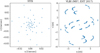 |
Fig. 1 Exemplary comparison of the STIX (u, υ) (left panel) and of the EHT (right panel; Event Horizon Telescope Collaboration 2019a,b) coverage. In both cases, the Fourier domain is undersampled, although the degree of undersampling is more enhanced in the STIX case. |
2 Theory
In this section, we present the basic notions of VLBI and STIX imaging. The concepts here presented are the bases for understanding the image reconstruction problem.
2.1 VLBI
The correlation product of an antenna pair in a VLBI array is approximately the Fourier transform of the true sky brightness distribution. This is described by the van-Cittert-Zernike theorem:
 (1)
(1)
where I(l, m) is the sky brightness distribution, and l, m represent the direction cosines. We typically ignore w-projection terms due to small field of view for VLBI. The observables 𝒱(u, υ) are called visibilities with respect to the harmonics, u, υ, determined by the baselines separating the antennas projected on the sky plane. When we produce an image in VLBI we are trying to recover the image intensity, I(l, m), from the measured visibilities. Since the Fourier domain (i.e., (u, υ) domain) is only sparsely sampled by observations, VLBI imaging constitutes an ill-posed inverse problem. The problem is further complicated by calibration effects and thermal noise. Particularly, the observed visibilities for an antenna pair, i, j, at a time, t, are related to the model visibilities by the relation:
 (2)
(2)
where Ni, j is Gaussian thermal noise with an unknown correlation structure and gi is complex valued gain factors specific to antenna, i. The gain factors typically vary over the time of an observation. While most VLBI algorithms were developed and are applied in the context of gain-corrupted data sets; for instance, by alternating imaging with self-calibration loops (hybrid imaging Readhead & Wilkinson 1978; Mus et al. 2022) or by closure only imaging (Chael et al. 2018; Müller & Lobanov 2022; Müller et al. 2023), we focus in this work on dealing with undersampling and noise corruption issues and ignore the need for self-calibration in VLBI.
2.2 STIX
The STIX instrument contains 30 sub-collimators, that is, units consisting of a grid pair and a detector mounted behind it. The period and orientation of the front and of the rear grid in each pair are chosen in such a way that the transmitted X-ray flux creates a Moiré pattern on the detector surface with period equal to the detector width (e.g., Hurford 2013; Prince et al. 1988). STIX Moiré patterns encode information on the morphology and location of the flaring X-ray source. Therefore, from measurements of the transmitted X-ray flux performed by the detector pixels, it is possible to compute the values of amplitude and phase of 30 complex visibilities (Massa et al. 2023).The imaging problem for STIX can then be described by the following equation:
 (3)
(3)
where j = 1,…, 30 is the sub-collimator index, 𝒱(uj, υj) is experimental visibility corresponding to the (uj, υj) angular frequency, and I(x, y) is the angular distribution of the intensity of the X-ray source. We note that, unlike the VLBI case, in the STIX case there is a plus sign inside the complex exponential that defines the Fourier transform (cf. Eqs. (1) and (3)). Furthermore, the angular frequencies sampled by STIX are only determined by geometric properties of the instrument hardware (Massa et al. 2023); therefore, they are the same for every recorded event.
STIX measures a number of visibilities which is at least an order of magnitude lower compared to that measured by VLBI. Therefore, the ill-posedness of the imaging problem for the X-ray imager is more enhanced compared to that of the radio domain. However, the great advantage of STIX is that the data calibration (in particular, the visibility phase calibration) depends only on the geometry of the sub-collimator grids and is therefore stable in time (Massa et al. 2023).
3 Imaging methods
In this paper, we compare the reconstructions from a variety of algorithms and algorithmic frameworks. We will briefly explain each of these frameworks in the following subsections. A tabular overview of the algorithms, their optimization details, their basic ideas, regularization properties, advantages, and disadvantages is presented in Appendix A.
3.1 CLEAN
CLEAN and its many variants (Högbom 1974; Wakker & Schwarz 1988; Schwarz 1978; Bhatnagar & Cornwell 2004; Cornwell 2008; Rau & Cornwell 2011; Offringa & Smirnov 2017; Müller & Lobanov 2023b) are the de-facto standard imaging methods for VLBI and STIX. CLEAN reformulates the imaging problem as a deconvolution problem by means of the dirty beam BD and dirty map ID. The former is the instrumental point spread function (PSF), while the latter is the inverse Fourier transform of the all measured visibilities sampled on an equidistant grid, filled by zeros for every non-measured Fourier coefficients (i.e., for gaps in the (u, υ) coverage) and reweighted by the noise ratio (natural weighting) or the power within a grid-ding cell (uniform weighting) or a combination of both (Briggs 1995). In this way, CLEAN solves the problem:
 (4)
(4)
In the classical CLEAN (Högbom 1974), this problem is solved iteratively in a greedy matching pursuit process. In a user-defined search window, we searched for the maximal peak in the residual, stored the position and strength of the peak in a list of CLEAN components, shifted the dirty beam to the position of the peak, and subtracted a fraction of the beam (determined by the CLEAN gain) from the residual. This procedure was repeated with the new residual until the residual is noise-like, namely, we computed the following approximation:
 (5)
(5)
with ai being the intensity of the i-th CLEAN component, and li, mi the coordinates of its location. Finally, using BC to denote the CLEAN beam, namely, a Gaussian beam that is fitted to the central lobe of the dirty beam, the final CLEAN image is computed by convolving the CLEAN components with BC:
 (6)
(6)
It is also standard to add the last residual to the reconstructed image to account for any non-recovered flux. While CLEAN remains in use, mainly because it is straightforward and interactive, it remains fairly limited (e.g., see the recent summaries on the limitations of CLEAN; Pashchenko et al. 2023; Müller & Lobanov 2023c). We summarize some of the main limitations of CLEAN here. The representation of the image by a sample of point sources is not a reasonable description of the physical image, particularly when representing extended emission. This issue has two important consequences. First, the model that is fitted to the data (i.e., CLEAN components) and the final image (CLEAN components convolved with the clean beam) are not the same. Particularly, for high dynamic range imaging, we would therefore self-calibrate the image to a model that was deemed physically unfeasible. Second, the representation of the image by CLEAN components makes the use of a final convolving necessary, thus limiting the effective resolution. Moreover, the value of the full width at half maximum (FWHM) of the Gaussian beam utilized in the final convolution is a parameter that has to be arbitrarily selected by the user, although estimates on maximum baseline coverage are usually adopted. As a consequence, CLEAN is a strongly supervised algorithm. It is key to the success of CLEAN for the astronomer performing the analysis to build their perception of image structure in an interactive way; namely, by changing the CLEAN windows, gain, taper, and weighting during the imaging procedure. This makes CLEAN reconstructions often challenging to reproduce.
Multiple of these issues can be effectively solved by recently proposed variants of the standard CLEAN algorithm (e.g., Müller & Lobanov 2023b; Perracchione et al. 2023). The classical way to increase resolution for CLEAN is by updating the weights, for instance, to uniform or even super-uniform weighting. Since most interferometric experiments have a higher density of short baselines rather than long ones, this leads to an overweighting of large-scale structures at the sake of resolution. Uniform weighting, or any hybrid weighting in between (Briggs 1995), addresses this fact by giving a larger weight to the long baselines, at the cost of the overall structural sensitivity.
The U-CLEAN algorithm recently proposed by Perracchione et al. (2023) combines the CLEAN method with an extrapolation/interpolation scheme that allows for a more automated CLEAN procedure. Specifically, the method utilizes the Fourier transform of the CLEAN components as a priori information for performing a reliable interpolation of the real and the imaginary parts of the visibilities. This feature augmentation technique is particularly useful for image reconstruction from STIX data since, in that case, the interpolation task suffers from the extreme sparsity of the (u, υ) coverage. Once the visibility interpolation step is completed, image reconstruction is performed by minimizing the reduced χ2 between the interpolated visibility surface and the Fourier transform of the image via a projected Landweber algorithm (Piana & Bertero 1996).
DoB-CLEAN is a recently proposed multiscalar CLEAN variant (Müller & Lobanov 2023b) that models the image by the difference of elliptical Bessel functions (DoB-functions), which are fitted to the (u, υ) coverage. CLEAN is not used as a deconvolution algorithm, but as a feature finder algorithm. The cleaning of the image is performed by switching between the DoB-dictionary to a dictionary consisting of the difference of elliptical Gaussian functions. Both DoB-CLEAN and U-CLEAN waive the necessity for the final convolution of the CLEAN components with the CLEAN beam (Müller & Lobanov 2023b; Perracchione et al. 2023); hence, the algorithms are not biased by the arbitrary choice of the CLEAN beam FWHM.
3.2 Maximum entropy
Historically, maximum entropy methods (MEM) were among the first algorithms that were proposed for imaging (e.g., Frieden 1972; Ponsonby 1973; Ables 1974). Despite its relative age, MEM was disfavored in practice in comparison to CLEAN. However, there are a number of active developments for MEM-based algorithms (e.g., Massa et al. 2020; Mus & Martí-Vidal 2024). Many of them reinterpret the MEM functional as one of many objectives in forward modeling frameworks (Chael et al. 2016, Chael et al. 2018; Müller et al. 2023; Mus et al. 2024). These algorithms are based on the constrained optimization framework (originally presented in Cornwell & Evans 1985) or on the unconstrained optimization setting.
MEMs are regularization techniques that use a large image entropy as a prior information, namely, among all the possible solutions that could fit the data, the most simple (in the sense of information fields) is selected. If I = I (x) and G = G (x), the entropy is measured by the Kullback–Leibler divergence functional (Kullback & Leibler 1951):
 (7)
(7)
where G is a possible prior image. Common priors include “flat” priors (i.e., a constant image is rescaled in such a way that the sum of the pixels is equal to a priori estimate of the total flux) or Gaussian images corresponding to the size of the compact flux emission region of the image structure. To ensure that the proposed guess solution fits the data, the value of the reduced χ2 data-fitting metric is constrained. In particular, the problem presented in Cornwell & Evans (1985) is:
 (Cons_MEM)
where V is the array of visibilities, ℱ is the forward operator (undersampled forward operator), Fmod is the model flux, and Ω is the noise estimation. To satisfy the non-negativity of the solution, we modeled the image by a lognormal transform, which is a strategy that has become popular in Bayesian algorithms (Arras et al. 2019, 2021).
From the optimization viewpoint, the main disadvantage of the problem (Cons_MEM) is its non-convexity, given the quadratic equality constraint defined by the reduced χ2. Therefore, Massa et al. (2020) defined a new version of the maximum entropy problem, named MEM_GE, in which the objective function is a weighted sum of the reduced χ2 and of the negative entropy functional:
 (MEM_GE)
where λ is the regularization parameter balancing the tradeoff between data-fitting and regularization. Furthermore, in the MEM_GE implementation, G is chosen as a “flat” prior. The optimization problem (MEM_GE) is convex and can be solved by standard optimization techniques. Specifically, Massa et al. (2020) adopted an accelerated forward-backward splitting (Beck & Teboulle 2009; Combettes & Pesquet 2011). We note that the MEM_GE approach is similar to regularized maximum likelihood approaches (cf. Sect. 3.3). However, the latter often combines several regularization terms and therefore makes a single description by a proximal point minimization method more challenging. Therefore, the minimization techniques that are typically adopted in RML approaches are gradient descent, conjugate gradient (CG), or limited-memory BFGS (L-BFG-S) (Hestenes & Stiefel 1952; Liu & Nocedal 1989). In this paper (among aspects), we compare the latter strategy for entropy objectives (RML_MEM) with the MEM_GE approach. A further difference between MEM_GE and RML approaches is in the assumed prior distribution (“flat” prior versus Gaussian prior) and in the automatic stepsize and balancing update developed for MEM_GE (Massa et al. 2020).
3.3 Regularized maximum likelihood
Regularized maximum likelihood (RML) methods approach the imaging problem by balancing data fidelity terms and regular-ization terms, namely, by solving an optimization problem that takes the form:
 (8)
(8)
where V represents the observed visibilities, ℱ the forward operator (undersampled Fourier transform), Si the data fidelity terms, and Rj the regularization terms. Also, αi,βj ∈ ℝ+ are the regularization parameters that control the balancing between the different terms. The data fidelity terms measure the fidelity of the guess solution, I, and the regularization term measures the feasibility of the solution according to the perception of the image structure. The usual data fidelity terms are reduced χ2-metrics between the observed visibilities and the predicted visibilities. For VLBI, the use of calibration independent closure quantities has become more common (Chael et al. 2018; Müller & Lobanov 2022; Müller et al. 2023), but for this work, we use the reduced χ2-metric to the visibilities. The regularization terms encode various prior assumptions on the feasibility of the image, for instance, simplicity (l2-norm), sparsity (l1-norm), smoothness (total variation, hereafter, TV, and the total squared variation), maximal entropy (Kullback–Leibler divergence), or a total flux constraint. For a full list of regularization terms that were used in VLBI we refer the interested reader to the discussions in Event Horizon Telescope Collaboration (2019b). While RML methods are expected to produce excellent, super-resolving images (Roelofs et al. 2023; Event Horizon Telescope Collaboration 2019b), they depend strongly on the correct regularization parameter selection, αi, βj. For the sake of simplicity, we focus on entropy, sparsity and total variation terms for this paper. Thus, we chose a representative (but not necessarily ideal) parameter combination. In particular, we tested the following approaches:
 (9)
(9)
with respective regularization parameters, α, β, γ. In practice, we need to ensure that the pixels are not negative. This is handled by the lognormal transform, namely, apply the change of variables I ↦ exp I, before evaluating the Fourier transform (Chael et al. 2018; Arras et al. 2022). The prior for the entropy functional G is chosen as a Gaussian whose full width at half maximum (FWHM) is consistent with the size of the compact emission region. The size of the compact emission region may be evaluated in practice from multiwavelength studies of the source (Event Horizon Telescope Collaboration 2019b).
3.4 Compressive sensing
Compressive sensing (CS) is aimed at sparsely representing the image in a specific basis. Typically wavelets have been used for this task (e.g., see Candès et al. 2006; Donoho 2006; Starck & Murtagh 2006; Starck et al. 2015; Mertens & Lobanov 2015; Line et al. 2020, for an application within radio interferometry). The sample of basis functions is called a dictionary, Γ, while the single basis functions are called atoms. In the following, we show how we chose Γ as a wavelet dictionary. The idea behind the CS technique is to represent the image as a linear combination of the atoms, namely, I = ΓI, and to recover the array of coefficients, I, by solving:
 (10)
(10)
Such algorithms and many variants have been studied in radio interferometry for a long time (Weir 1992; Bontekoe et al. 1994; Starck et al. 1994, 2001; Pantin & Starck 1996; Maisinger et al. 2004; Li et al. 2011; Carrillo et al. 2012, 2014; Garsden et al. 2015; Girard et al. 2015; Onose et al. 2016, 2017; Cai et al. 2018a,b; Pratley et al. 2018; Müller & Lobanov 2022, 2023b). For the comparison that was carried out for this work, we consider the DoG-HiT algorithm that was recently proposed by Müller & Lobanov (2022, 2023c). Difference-of-Gaussian (DoG) hard iterative thresholding (DoG-HiT) utilizes DoG wavelet functions. For DoG-HiT, the basis functions are fitted to the (u, υ) coverage, hence, they are optimally separating the measured and non-measured Fourier coefficients. The minimization problem is solved with an iterative forward-backward splitting technique. The algorithm has been proven to recover images of comparable quality as RML methods (Müller & Lobanov 2022; Roelofs et al. 2023), although the optimization landscape is much simpler. With only one free regularization parameter, DoG-HiT is a substantial step towards an unsupervised imaging algorithm without the need for large parameter surveys. Originally, DoG-HiT was proposed for closure-only imaging; for this comparison, we fit the visibilities directly instead.
3.5 Multiobjective imaging
Multiobjective optimization (MOEA/D) is a recently proposed (Müller et al. 2023; Mus et al. 2024) imaging algorithm for VLBI. It mimics the formulation of the imaging problem in the RML framework, namely, with a set of data fidelity terms and regularization terms. However, instead of solving a weighted sum of these terms as in Eq. (8), we have solved a multiobjective problem consisting of all the regularizers and data terms as single objectives (for more details, we refer to Müller et al. 2023). A solution to the multiobjective problem is called Pareto optimal if the further optimization along one objective automatically leads to the worsening of another one. The set of all Pareto optimal solutions is called the Pareto front. MOEA/D recovers the Pareto front. Since several regularizers introduce conflicting assumptions (i.e., sparsity in comparison to smoothness) the Pareto front divides into a number of disjunct clusters (Müller et al. 2023), everyone describing a locally optimal mode of the multimodal reconstruction problem. In this spirit, it is not the goal of MOEA/D to recover a single image, but to recover a full hyper-surface of image structures. This is most easily realized with the help of evolutionary algorithms (Zhang & Li 2007; Li & Zhang 2009). In order to select the (objectively) best cluster of representative solutions, we applied the accumulation point selection criterion proposed in Müller et al. (2023), namely: we selected the cluster of images that has the largest number of members in the final population.
3.6 Bayesian Imaging
Bayesian reconstruction methods have been intensively studied in radio interferometry (e.g., see Junklewitz et al. 2016; Cai et al. 2018a,b; Arras et al. 2019, 2021, 2022; Broderick et al. 2020b,a; Tiede 2022; Roth et al. 2023; Kim et al. in prep.). Bayesian imaging methods calculate the posterior sky distribution 𝒫(I|V) from the prior distribution 𝒫(I) and visibility data V by Bayes’ theorem:
 (11)
(11)
where 𝒫(V|I) is the likelihood distribution and 𝒫(V) is the evidence. The prior distribution contains prior knowledge on the source I, such as the positivity and smoothness constraints, while the likelihood represents our knowledge of the measurement process.
In Bayesian imaging, instead of obtaining an image, samples of possible images are reconstructed; therefore, it allows us to estimate the mean and standard deviation from the samples. Bayesian imaging has a distinctive feature: the uncertainty information in the visibility data, V, domain can be propagated in other domains. As a consequence, the reliability of reconstructed parameters, such as the image, I, and antenna gain, can be quantified by the uncertainty estimation.
Bayes’ theorem can be written by the negative log probability, also called the energy or Hamiltonian, ℋ (Enßlin 2019):
 (12)
(12)
The maximum a posteori sky posterior distribution of I is determined by minimizing an objective function containing the likelihood and prior:
 (13)
(13)
where ℋ(V|I) is the likelihood Hamiltonian and ℋ(I) is the prior Hamiltonian. We note that the evidence term is ignored in the objective functional since it does not depend on the sky brightness distribution of I.
From the posterior sky brightness distribution 𝒫(I\V), we can calculate the posterior mean:
 (14)
(14)
We note that the reconstructed image in this work is the posterior sky mean of I. Furthermore, the standard deviation of sky for I can be analogously calculated from the posterior distribution, 𝒫(I|V). The standard deviation allows us to quantify the reliability of reconstructed results.
Bayesian inference requires substantial computational resources in order to obtain the posterior probability distribution instead of a scalar value for each parameter. For instance, sampling by a full-dimensional Markov chain Monte Carlo (MCMC) procedure or evalutaing the high-dimensional integrals of the mean directly can often take too much time (Cai et al. 2018a,b).
In this work, images are reconstructed by means of the Bayesian imaging algorithm resolve. In order to perform a high-dimensional image reconstruction, variational inference (VI) methods (Knollmüller & Enßlin 2019; Frank et al. 2021) are used in resolve. In the variational inference method, the Kullback–Leibler divergence (Kullback & Leibler 1951) is minimized in order to find an approximated posterior distribution as closely as the true posterior distribution. Although the uncertainties tend to be underestimated in the VI method, it enables us to estimate the high-dimensional posterior distribution. In conclusion, it strikes a balance between the performance of the algorithm and the statistical integrity.
Bayesian imaging shares some similarities with RML approaches, in the sense that the RML methods can be interpreted as the maximum a posteriori (MAP) estimation in Bayesian statistics. The negative log-likelihood function, ℋ(V/I)in Eq. (13) is equivalent to the data fidelity term and the negative log-prior, ℋ (I), can be interpreted as the Bayesian equivalent to the regularizer in RML methods (Kim et al., in prep.). For instance, the correlation structure between image pixels can be inferred by Gaussian process with non-parametric kernel in resolve (Arras et al. 2021). The unknown correlation structure can be inferred by the data, which plays a similar role as a smoothness prior in RML methods.
4 Challenge
4.1 Synthetic data sets
To test this variety of algorithmic frameworks, we compared our results to a set of synthetic data. These include typical image structures that could be expected for the STIX and the EHT instruments. In particular, we study the following synthetic data sets.
STIX synthetic data sets replicate a solar flare. To mimic spatial features that may be expected for observations with STIX, we simulated a double Gaussian structure and a loop shape (see Volpara et al. 2022, for more details on the definition of the considered parametric shapes). In particular, the double Gaussian structure represents typical non-thermal X-ray sources at the flare footpoints, while the loop shape represents a thermal source at the top of the flare loop. Furthermore, the two Gaussian sources have different size and different flux: the left source has a FWHM of 15 arcsec and flux equal to 66% of the total flux, while the right source has a FWHM of 10 arcsec and flux equal to 33% of the total flux. We generated synthetic STIX visibilities corresponding to these configurations by computing their Fourier transform in the frequencies sampled by STIX. For the experiments performed in this paper, we only considered the visibilities associated with the 24 sub-collimators with coarsest angular resolution. Indeed, the remaining six sub-collimators have not yet been considered for image reconstruction, since their calibration is still under investigation (Massa et al. 2022).
We added an uncorrelated Gaussian noise to every visibility. To study the effect of the noise level on the final reconstruction, we prepared three different data sets with varying noise levels. We note that statistical errors affecting the STIX visibilities are due to the Poisson noise of the photon counts recorded by the STIX detectors. We simulated three different levels of data statistics corresponding to a number of counts per detector equal to ~500, ~2500, and ~5000. These data statistics will be referred to as low signal-to-noise ratio (low S/N), medium S/N, and high S/N for the remainder of the paper. Then, we added Gaussian noise to the visibilities with a standard deviation that is derived from the Poisson noise affecting the count measurements, resulting in an effective median S/N of ≈5, 12, and 16, respectively. Due to the small number of visibility points for STIX, the reconstruction is sensitive to the random seed of the random noise distribution. To get a statistical assessment on the reconstruction quality, we recovered the images from ten different realizations of the STIX data with a varying seed for the random noise distribution and average the results. In Figs. 2 and 3, we show the average over the ten reconstructions.
Since the similarity between STIX and VLBI imaging is greatest (in terms of accessible dynamic range, spatial scales, and degree of undersampling) when the VLBI (u, υ) coverage is sparsest and this is the data regime that has undergone the rapid development of novel methods that we are scrutinizing in this work (e.g., Chael et al. 2016, 2018; Akiyama et al. 2017b,a; Arras et al. 2022; Müller & Lobanov 2022, 2023b; Müller et al. 2023; Mus & Martí-Vidal 2024), we focus here on geometric models that mimick EHT observations. In fact, we have focused our study on a crescent geometric model. This model is a simple geometric approximation to the first image of the shadow of the supermassive black hole in M87 presented by Event Horizon Telescope Collaboration (2019a). It was specifically used for the verification of the imaging strategies for the analysis of M87 (Event Horizon Telescope Collaboration 2019b), as well as SgrA* (Event Horizon Telescope Collaboration 2022). We added thermal noise that is consistent with the system temperatures reported in Event Horizon Telescope Collaboration (2019b) and we assume that the phase and amplitude calibration are known.
The next generation EHT (ngEHT) is a planned extension of the EHT that is supposed to deliver transversely resolved images of the black hole shadow (Doeleman et al. 2019; Johnson et al. 2023). In order to test the algorithmic needs of this future frontline VLBI project, we also considered the synthetic data inspired by the first ngEHT analysis challenge presented by Roelofs et al. (2023). We used a general relativistic magneto-hydrodynamic (GRMHD) simulation of the supermassive black hole M87 (Mizuno et al. 2021; Fromm et al. 2022). We generated a synthetic set of data corresponding to the proposed ngEHT configuration, which consists of the current EHT antennas and ten additional proposed antennas (for more details, see, e.g., Raymond et al. 2021; Roelofs et al. 2023). We added thermal noise and assumed a phase and amplitude calibration. For VLBI, due to the larger number of visibilities with uncorrelated Gaussian noise contribution, we do not need to study several realizations of the noise contribution.
STIX and VLBI (and particularly EHT) utilize various astronomical conventions, data formats, software packages, and various programming languages for the respective data analysis. To transfer the STIX data sets into a VLBI framework, we created a virtual VLBI snapshot observation that has exactly the same (u, υ) coverage as STIX; and vice versa, we extract the (u, υ) coverage, visibilities, and noise ratios from the VLBI observations, saving the related data arrays and matrices in a readable format for STIX.
4.2 Comparison metrics
We compared the reconstruction results to the ground truth images using three different metrics, inspired by the metrics that were used in the recent imaging challenge presented by Roelofs et al. (2023). First (and most importantly) we computed the match between the ground truth images and the recovered images by means of the cross correlation:
 (15)
(15)
where IGT and IR represent the ground truth and the recovered image, respectively, 〈·〉 denotes the mean of the image pixel values, and σ is their standard deviation. This metric has been used in the past to determine the precision of VLBI algorithms in the framework of the EHT (Event Horizon Telescope Collaboration 2019b; Roelofs et al. 2023).
Moreover, we calculated the effective resolution of a reconstruction. Since the reconstructions are typically more blurred than the ground truth image, we determined the effective resolution via the following strategy. We blurred the ground truth image gradually with a circular Gaussian beam and computed ρ between the recovered image and the blurred ground truth image. We did this for a predefined set of blurring kernels and selected the one that maximizes ρ.
Finally, we determined the dynamic range with a strategy inspired by the proxy proposed in Bustamante et al. (2023). To have an approximation for the dynamic range that is independent of the resolving power of an algorithm, we first blurred every recovered image to the nominal resolution θnom, namely, the width of the clean beam. We did this in a similar way to the approach we used to estimate the image resolution. We gradually blurred the recovered images with a blurring kernel and calculated the cross correlation ρ between the blurred recovered image and the ground truth image, which had been blurred with the nominal resolution. Finally, we blurred the recovered images with the beam (Gaussian with width θres) that maximizes the correlation to the true image at nominal resolution. Then we computed the proxy of the dynamic range in the image:
 (16)
(16)
where 𝒢θ denotes a circular Gaussian with standard deviation equal to θ. We obtained the qth quantile of 𝒟, where we chose q = 0.1 in consistency with Roelofs et al. (2023); Bustamante et al. (2023):
 (17)
(17)
The numerical complexity of an algorithm is an additional important benchmark. We note that imaging algorithms proposed for VLBI (and radio interferometry in general) were historically proposed for bigger arrays with a larger number of visibilities, rendering them relatively fast in a STIX setting, comparable in speed to the algorithms that were proposed for STIX directly. The running time of the single algorithms (once the hyperparameters are fixed) is not a concern, as it allows for nearly real time image analysis due to the small number of visibilities that were adapted for these examples. In this paper, we do not touch on the question how well the various algorithms scale to bigger data sizes as are common for denser radio interferometers in general. With a relatively small computational effort to evaluate the model visibilities, the time for user-interaction and finetuning of the software specific hyperparameters becomes more relevant to the overall time that is consumed for the reconstructions.
Some algorithms, for example, DoG-HiT, MOEA/D, Cons_MEM, and MEM_GE, allow for an automatized imaging with minimal interaction, while other algorithms depend on a finetuning of a varying number of hyperparameters (e.g., RML and Bayesian algorithms), or manual interaction (CLEAN). Given these considerations, it is challenging to assign a quantitative metric on the numerical and application complexity of the algorithms, since the actual time needed to set up and run the algorithms is prone to external factors such as the quality of the data set or the experience of the user. Therefore, we opted for a qualitative comparison for the computational resources needed and reported on our experiences with the various data sets and imaging algorithms.
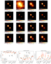 |
Fig. 2 Reconstruction results and scoring of the various imaging algorithms on the double Gaussian source model for STIX. In the upper panel, we show the reconstruction results for medium noise levels. In the lower panels, we compare the scoring of the reconstructions across various methods and noise-levels: the lower left panel shows the correlation, the lower middle panel the resolution and the lower right panel the dynamic range. Cons_MEM is over-resolving the source. |
4.3 Results
The data sets were independently analyzed in a semi-blind way with the algorithm presented in Sect. 3. The reconstruction results are shown in Figs. 2–5. Below, we provide a more detailed description of the performances of the methods, grouping them into their respective categories.
CLEAN-type algorithms. CLEAN is shown to exhibit a worse level of performance in terms of accuracy compared to all the other algorithms considered in the challenge, as proven by the systematically lowest correlation values (see panel b of Figs. 2–5 and panel a of Fig. 6). When inspecting the achieved spatial resolutions (panel c of Figs. 2–5 and panel b of Fig. 6), it becomes clear that the worse performance of CLEAN is directly related to its suboptimal resolution. While CLEAN has a well defined resolution limit (determined by the central lobe of respective point-spread function), it has been recognized both in VLBI (e.g., Lobanov 2005; Honma et al. 2014) and for STIX (e.g., Massa et al. 2022; Perracchione et al. 2023) that this limit is too conservative in the presence of strong prior information. Lobanov (2005) provided an analytic proxy for the resolution limit of an interferometric observation. While this resolution is only achievable in a specific model-fitting setting, namely, when constraining the possible source features to Gaussian model components, it demonstrates that more sophisticated regularization methods may enable super-resolution imaging. As we will discuss below, this is in particular achieved for the entropy-based methods (MEM_GE, MEM, Cons_MEM), sparsity promoting algorithms (l1) and the Bayesian reconstructions (resolve).
There are several available extensions of CLEAN that allow for super-resolution imaging. Classically, the issue of resolution is addressed by varying the CLEAN weights associated to the visibilities; we refer to Briggs (1995) for a complete overview. Moreover, recently novel CLEAN variants were proposed both for STIX and VLBI that achieve super-resolution by solving the disparity between the image and the model; namely, by making the unphysical convolution with the beam unnecessary, for instance, DoB-CLEAN (Müller & Lobanov 2023b) and U-CLEAN (Perracchione et al. 2023). U-CLEAN is included in the overall comparison, and performs very well compared to CLEAN by outperforming CLEAN in terms of resolution, accuracy, and dynamic range for all source models and experimental configurations.
In Fig. 6, we compare the performance of various CLEAN methods (CLEAN with natural weighting, CLEAN with uniform weighting, U-CLEAN and DoB-CLEAN) in more detail for the double Gaussian source in the case of the low, medium, and high S/N. For benchmarking, we also show the reconstruction quality of two of the best performing algorithms again, resolve, and MEM_GE. Changing the weighting scheme is improving the scoring of the CLEAN algorithm. However, this standard (and often performed, albeit rather simple) trick does not bring the same amount of improvements that more sophisticated interferences (such as those realized within U-CLEAN and DoB-CLEAN) offer. U-CLEAN achieves slightly higher resolutions than DoB-CLEAN, while DoB-CLEAN achieves slightly higher dynamic ranges. While these approaches show significant improvements to standard CLEAN, they do not perform as well as the best available forward-modeling approaches.
CLEAN remains the de facto standard method for VLBI and STIX reconstructions, partly due to its speed. The Fourier transform only needs to be evaluated in the major cycles, while the minor cycles only comprise of fast array substitution operations.
As a consequence of the small number of pixels and the relatively simple source structures, the CLEAN reconstructions had a numerical running time of approximately 30 s on a standard notebook. However, CLEAN lacks a strictly defined stopping rule. Hence, the exact time of execution depends on the manually fixed number of iterations. On the other hand, DoB-CLEAN and U-CLEAN incorporate more complex operations with extended basis functions. This slows the data analysis down considerably, taking up to 15 min for DoB-CLEAN for STIX data sets. It should be noted here that when using CLEAN-like algorithms, a considerable chunk of time is devoted to interactive choices done by the astronomer, most importantly, the selection of the CLEAN windows. For the examples studied in this work this considerable effort has been waived since the ground truth models are compact and rather simple and former experiences with disk masks as explored by the EHT (Event Horizon Telescope Collaboration 2019b) existed and were utilized. The reconstruction in a completely blind, more complex data-set may take considerably longer.
Maximum entropy methods. Inspecting the cross correlation metric ρ for the STIX data sets, the entropy-based methods perform best. There are only marginal differences between the different versions of entropy maximization, namely, between Newton type minimization and forward-backward splitting. Cons_MEM tops the performance overall for low-S/N data, but performs less effectively for higher S/N data compared to MEM_GE. This correlates with the relatively small dynamic ranges recovered for Cons_MEM in these cases. We note that the dynamic range was computed at a common resolution (i.e., CLEAN resolution). The performance of Cons_MEM may be explained by the fact that regularization is less strictly employed at low S/N, since the squared programming still requires reduced χ2 = 1, even for data that are highly corrupted with noise, while accounting for the fact that Cons_MEM tends to overresolve the source structure. It reconstructs structures on scales smaller than the ground truth. The regularization assumption, balancing of the Lagrange multipliers, and (possibly) the lognormal representation of the model bias the reconstruction towards shrinked structures. This behaviour, which will be also detected for sparsity promoting RML algorithms (l1), is a warning sign to accept super-resolved structures only with relative caution, although it is not necessarily mirrored in the metrics presented. It is however notable that this is not an uncommon situation for imaging sparsely sampled Fourier data in the sense that it is similar to CLEAN philosophy. It may be shown that CLEAN is effectively a sparsity-promoting minimization algorithm (Lannes et al. 1997) that over-resolves the image drastically, which makes a final convolution with the clean beam as a low-pass filter necessary.
MEM_GE performs significantly better than CLEAN, but worse than RML methods for the VLBI data sets (and was more complicated to apply in practice). This is not unexpected given the much larger number of visibilities and the wide range of existing spatial scales in the image, especially for the GRMHD image. While MEM_GE still recovers the overall structure significantly better than CLEAN, the reconstruction of the crescent observed with an EHT configuration shows some artifacts (non-closed crescent, spurious background emission that limits the dynamic range). We note that MEM_GE is equipped with a tailored rule for the regularization parameter selection when applied to STIX data (Massa et al. 2020). However, the same rule is not applicable to VLBI data and, therefore, an ad hoc choice of the regularization parameter has been adopted for reconstructing the images shown in Figs. 4 and 5.
We would like to highlight the remarkable performance of the plain MEM method with the crescent EHT data set, whereby it seems to outperform the alternative MEM_GE approach and even Bayesian imaging. This improved performance may be attributed to the adopted form of the entropy functional. For MEM_GE, a flat prior has been used, for plain MEM a Gaussian with the size of the compact emission region. This resembles a strategy that was applied by the EHT, where the size of the compact emission is constrained as an additional prior information from independent observations at smaller frequencies (Event Horizon Telescope Collaboration 2019b). In particular, it has been demonstrated that the size of the Gaussian prior for the computation of the entropy functional plays a significant role in the reconstruction (compare the dropping percentage of top-sets for varying sizes presented in Event Horizon Telescope Collaboration 2019b).
Maximum entropy methods, as well as the closely related RML reconstructions, have a small numerical complexity due to the small number of visibilities and the efficacy of the limited BFGS (respectively the SQP minimization for Cons_MEM) optimization techniques. For the STIX examples the numerical runtime took roughly a minute on a common notebook and extends up to 3 min for the more complex ngEHT setting, indicating a proper scaling to a larger number of visibilities. It is further noteworthy (as mentioned above) that MEM_GE is equipped with a tailored rule to select the regularization parameter and Cons_MEM is free of any tunable regularization parameters at all, marking them as remarkably fast and simple to use algorithms in practice.
Bayesian reconstruction method. While the resolve algorithm may be outperformed by alternative approaches in some examples, for instance, by DoG-HiT for the EHT or by MEM_GE in the case of STIX data, it is among the best algorithms across all instances and metrics. In particular, it shows to be an interdisciplinary alternative since it performs equally well for VLBI and STIX data analyses. Bayesian reconstructions add the additional benefit of a thorough uncertainty quantification, however, at the cost of an increased complexity and computational resources (see our comparison in Appendix A). The probabilistic approach can be beneficial for the robust image reconstruction from sparse and noisy VLBI and STIX data set.
Bayesian methods typically need more numerical resources than comparable approaches due to the sampling; however, resolve achieves a significant speed-up by means of the adoption of variational inference (VI) methods (Knollmüller & Enßlin 2019; Frank et al. 2021). Furthermore, we note that resolve is the only software included in this comparison which backend has been implemented in C++ rather than python (used for RML, MEM, DoG-HiT, and CLEAN) or IDL (used for MEM_GE) contributing further to a significant speed-up. For the STIX synthetic data sets, the computational time is around 2 min with 256 × 256 pixels and 6 min for EHT synthetic data set with 256 × 256 pixels. For the real STIX data sets, 512 × 512 pixels are used and the computational time is 6 min. By the standardized generative prior model in resolve, the independent Gaussian random latent variables are mapped to the correlated log-normal distribution. The Gaussian approximated latent variables are estimated by the minimization of the Kullback-Leibler divergence in the variational inference framework. The parametrization of the latent space makes it possible to achieve affordable high-dimensional image reconstruction, although multi-modal distribution cannot be described by approximated Gaussian distribution and the uncertainty values tend to be underestimated.
For the STIX real-data application, resolve dealt with 306 197 parameters in total; generally, resolve depends on a number of free parameters that need to be fixed manually. For the examples studied in this paper, there were l1 free parameters (compared to 1 free parameter for DoG-HiT and MEM and 3 for RML). However, only the range (mean and standard deviation) are fixed, not the exact values to ensure flexibility on the prior.
Compressive sensing technique. overall,DoG-HiT performs very well, outperforming CLEAN and most non-MEM RML methods (particularly with respect to the dynamic range; see panel d of Figs. 2–5). However, this technique shows a slightly worse resolution induced by the nature of the extended basis functions. In particular, we would like to highlight the performance of DoG-HiT for reconstructions with a EHT configuration, topping the performance in terms of accuracy (ρ) and an exceptionally high dynamic range. This is probably not surprising, since DoG-HiT was explicitly developed for the EHT (Müller & Lobanov 2022) and just recently saw promising application outside (Müller & Lobanov 2023c). DoG-HiT is an unsupervised and automatized variant of RML algorithms, it reduces the human bias to a minimum, making it easy and fast to apply in practice. However, the numerical resources are slightly higher. DoG-HiT needs approximately 5 min for the reconstruction of a single STIX data set, and roughly the same time for the denser ngEHT configuration. This efficient scaling to bigger data sets is caused by the fact that while the evaluation of the Fourier transform gets numerically more expensive with a larger number of visibilities, the number of wavelets needed to describe the defects of the beam decreases due to the better uυ coverage as well.
Multiobjective imaging method. MOEA/D is the only algorithm that explores the multimodality of the problem (see Appendix A). It finds clusters of locally optimal solutions. It computes a wide range of solutions for STIX ranging from very successful clusters comparable to entropy methods to worse reconstructions. The selection of the best cluster by the least-square principle or accumulation point criterion presented in Müller et al. (2023) however proved challenging. When applied to STIX data, MOEA/D provides good quality reconstructions. However, it reveals to be less promising than resolve when applied to hard X-ray visibilities. Since MOEA/D (in contrast to the other imaging algorithms described in this paper) does not compute a single solution, but a sample of possible image features instead, the numerical resources are comparably high. It took 90 min to reduce a single STIX data set and more than 4 h for the ngEHT configuration on a common notebook. There are however multiple considerations that need to be taken into account when putting these running times into context. First, the application is automatized and free of human interaction, namely, adding no additional time for the setup of the algorithm. Second, MOEA/D works with the full set of regularizers, also including l2 and total squared variation that were omitted for the RML approaches for the sake of simplicity. Lastly, a convergence analysis showed that the algorithms may have converged already after 200 rather than 1000 iterations such that the numerical running time may have been severely overestimated.
Regularized maximum likelihood methods. instead of a thorough parameter survey with all the data terms and regularization terms for RML, we study only a representative selection of terms for this paper inspired by the balacing principle, namely, the scoring of all regularization terms were of similar size. In fact, the regularization terms were chosen manually for a good performance. The impact of the regularization terms is as expected and as reported in the literature; also, l1 promotes sparsity, thus super-resolution. TV promotes piecewise constant filaments connected by smooth functions. An entropy term promotes simplicity of the solution. For RML methods, all these terms need to be balanced properly. This leads to a high number of free hyperparameters, which stands as a severe drawback. This is typically tackled by parameter surveys, namely, by the exploration of the scoring of the method with different weightings on synthetic data. This strategy was successfully applied in Event Horizon Telescope Collaboration (2019b, 2022) and demonstrated the robustness of the reconstruction, but it is still a lengthy and time-consuming procedure. While RML methods rank among MEM methods with respect to the numerical complexity (i.e., it just takes several minutes to recover a solution), the parameter survey may take significant time depending on the number of competing regularization terms that need to be surveyed. In the case of the EHT, this procedure added up to 37 500 parameter combinations that needed to be surveyed Event Horizon Telescope Collaboration (2019b). Without parallelization, this would add up to more than 20 days of computation, but in reality always a parallel computing infrastructure is utilized. For this paper, we opted for a simpler approach by manually selecting well working weights by a visual inspection of keytrends on synthetic data sets. Adaptive regularization parameter updates (e.g., as for MEM_GE Massa et al. 2020), multiobjective evolution (as realized for MOEA/D, see Müller et al. 2023), or the choice of more data-driven regularization terms (e.g., as for DoG-HiT, see Müller & Lobanov 2022,2023c) were recently proposed to solve the issue of lenghty parameter surveys towards an unsupervised imaging procedure. When applied to STIX data, l1 and MEM_l1 prove to be the best performing among all the RML methods with respect to the three metrics. In particular, they achieve dynamic range values among the highest ones within the challenge. However, a visual inspection of the reconstructions (see Figs. 2 and 3) shows a shrinking effect in the l1 reconstructions, in line with the sparsity promoting property of the method. This may possibly indicate an overestimated regularization parameter that led the regularization term dominate the reconstruction. The good performances of the RML methods are confirmed when applied to VLBI data, although in this case, the differences between performances of the various regularization terms are less pronounced.
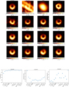 |
Fig. 4 Reconstruction results and scoring of the various imaging algorithms on the crescent source model observed with the EHT configuration. The upper panel compares the reconstructions, the lower left panel shows the correlation, the lower middle panel the resolution and the lower right panel the dynamic range. Note: resolution values are close to zeros for a few algorithms (Cons_MEM, MEM, l1 and MEM_l1) since they over-resolve the source, namely, they recover structures that are finer than those in the ground truth image due to too much enhancing of the regularizer. |
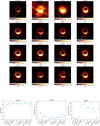 |
Fig. 5 Reconstruction results and scoring of the various imaging algorithms on the GRMHD source model observed with the ngEHT configuration. The upper panel compares the reconstructions, the lower left panel shows the correlation, the lower middle panel the resolution and the lower right panel the dynamic range. |
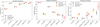 |
Fig. 6 Comparison of the reconstruction quality among different CLEAN variants (CLEAN, U-CLEAN, Clean with uniform weights, and DoB-CLEAN), benchmarked against bayesian reconstructions and reconstructions done with MEM_GE, in the case of the STIX double Gaussian configuration. The lower left panel shows the correlation, the lower middle panel the resolution and the lower right panel the dynamic range. |
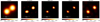 |
Fig. 7 Imaging results of SOL2023-05-16T17 event recovered with various algorithms (CLEAN, U-CLEAN, MEM_GE, resolve, and DoG-HiT, from left to right, respectively). |
4.4 Real data
As additional verification, we test selected algorithms (i.e., the best-performing methods and CLEAN for benchmarking) on a real data set observed with STIX. Specifically, we consider the SOL2023-05-16T17 event integrated in the time range 17:20:3017:21:50 and in the energy range 22–76 keV. We show the reconstruction results with five different algorithms in Fig. 7. All algorithms successfully identify a double-Gaussian structure. As discussed in the previous section in greater detail, the novel algorithms improve over CLEAN mainly by a higher resolution. All four algorithms considered here (i.e., two proposed by the STIX community and two provided by the VLBI community increase the resolution, and closely agree in terms of the super-resolved structure.
5 Discussion and conclusion
In this work, we explore the synergies between VLBI and STIX imaging. By cross-applying the proposed imaging algorithms and evaluating their performance, we have successfully demonstrated the strong synergies and rich opportunities of mutual interaction between the communities. This code-comparison is one of the most large-scale code comparisons carried out in the field to date, as it includes submissions by 17 different algorithms from a variety of algorithmic frameworks including inverse modeling, MEM, RML, and Bayesian approaches, as well as multiobjective evolutionary and compressive sensing. With the background of ongoing efforts regarding the development of novel imaging methods, we can identify some key trends that may lead future developments in the fields. Our main findings are as follows.
Modern imaging methods outperform CLEAN in terms of accuracy, dynamic range, and resolution in nearly all circumstances. The amount of additional physical information that could be extracted by more sophisticated imaging algorithm is significant, hence fostering the further development of modern imaging methods. There are long-standing and simple alternatives to the standard CLEAN procedure (e.g., varying the weighting scheme), which are in frequent use. However, significant improvements to the CLEAN strategy of imaging either requires deeper fixes to the inverse modeling pipeline as done by modern CLEAN variants (Müller & Lobanov 2023b; Perracchione et al. 2023) or completely changing the paradigm towards forward modeling techniques.
The VLBI side developed a wide range of RML imaging methods that deal with the multimodality of the problem (MOEA/D; Müller & Lobanov 2022) and work towards unsu-pervised imaging with a multiscalar imaging (DoG-HiT; Müller et al. 2023). While these automatized, blind imaging algorithms perform all well on STIX data sets outperforming CLEAN for a variety of data properties (i.e., noise levels), they do not outperform the data reconstruction algorithms with significantly simpler optimization landscape, faster numerical performance, and simpler use in practice; primarily with respect to MEM methods, such as MEM_GE (Massa et al. 2020). That may be an important hint for the future development of methods for STIX. Particularly, the compressive sensing algorithm DoG-HiT does not bring the same amount of improvements as it does in VLBI, since the coverage does not allow for the same kind of separation between covered and non-covered parts.
The overall best reconstructions for STIX were achieved with entropy based algorithms (forward-backward splitting, Newton type, and squared programming). Due to their additional relative simplicity, we recommend setting our focus the development on these methods rather than introducing the highly complex data terms recently proposed for VLBI. In this paper, we compare three entropy-based imaging algorithms that differ in the exact form how the entropy functional is defined, the selection of the regularization parameter and the minimization procedure. They show slightly varying performance in different settings, which demonstrates that the MEM approach is flexible enough to adapt to multiple situations. Bayesian imaging algorithm resolve (Arras et al. 2019, 2021, 2022) performs just as well both for STIX and for VLBI, thereby constituting a viable alternative all over the board.
For VLBI reconstructions, the amount of available data (i.e., the sampling of the Fourier domain) and the amount of testable spatial scales (ranging several orders of magnitude) is higher. It has been demonstrated that the best results are obtained with combining many priors (l1, TV, MEM, TSV for RML, prior distribution for Bayesian) rather than with a single penalization to adapt to the fine structure (Event Horizon Telescope Collaboration 2019b; Müller et al. 2023). On the contrary, we have to deal with the problems of finding the correct weightings and priors, along with a misidentification that may be prone to biasing the data, as was observed with over-resolved structures in case of sparsity promoting regularization. The STIX algorithm MEM_GE is strikingly successful as well, but it does not yet allow for the high fidelity reconstructions that had been proposed by RML or DoG-HiT specifically.
Acknowledgement
We thank the team of the ngEHT analysis challenge for providing the data set of the first ngEHT analysis challenge to us. This work was partially supported by the M2FINDERS project funded by the European Research Council (ERC) under the European Union's Horizon 2020 Research and Innovation Programme (Grant Agreement No. 101018682) and by the MICINN Research Project PID2019-108995GB-C22. H.M. and J.K. received financial support for this research from the International Max Planck Research School (IMPRS) for Astronomy and Astrophysics at the Universities of Bonn and Cologne. A.M. also thanks the Generalitat Valenciana for funding, in the frame of the GenT Project CIDEGENT/2018/021. E.P. acknowledges the support of the Fondazione Compagnia di San Paolo within the framework of the Artificial Intelligence Call for Proposals, AIxtreme project (ID Rol: 71708).
Appendix A Overview of the imaging methods
Tabellaric overview of the properties, advantages and disadvantages of imaging frameworks that are frequently used in VLBI and for STIX.
References
- Ables, J. G. 1974, A&AS, 15, 383 [NASA ADS] [Google Scholar]
- Aghabiglou, A., Terris, M., Jackson, A., & Wiaux, Y. 2023, in ICASSP 2023 - 2023 IEEE International Conference on Acoustics, Speech and Signal Processing (ICASSP), 1 [Google Scholar]
- Akiyama, K., Ikeda, S., Pleau, M., et al. 2017a, AJ, 153, 159 [NASA ADS] [CrossRef] [Google Scholar]
- Akiyama, K., Kuramochi, K., Ikeda, S., et al. 2017b, ApJ, 838, 1 [NASA ADS] [CrossRef] [Google Scholar]
- Arras, P., Frank, P., Leike, R., Westermann, R., & Enßlin, T. A. 2019, A&A, 627, A134 [NASA ADS] [CrossRef] [EDP Sciences] [Google Scholar]
- Arras, P., Bester, H. L., Perley, R. A., et al. 2021, A&A, 646, A84 [NASA ADS] [CrossRef] [EDP Sciences] [Google Scholar]
- Arras, P., Frank, P., Haim, P., et al. 2022, Nat. Astron., 6, 259 [NASA ADS] [CrossRef] [Google Scholar]
- Beck, A., & Teboulle, M. 2009, IEEE Trans. Image Process., 18, 2419 [CrossRef] [MathSciNet] [PubMed] [Google Scholar]
- Bhatnagar, S., & Cornwell, T. J. 2004, A&A, 426, 747 [NASA ADS] [CrossRef] [EDP Sciences] [Google Scholar]
- Bontekoe, T. R., Koper, E., & Kester, D. J. M. 1994, A&A, 284, 1037 [Google Scholar]
- Briggs, D. S. 1995, PhD thesis, New Mexico Institute of Mining and Technology, USA [Google Scholar]
- Broderick, A. E., Gold, R., Karami, M., et al. 2020a, ApJ, 897, 139 [Google Scholar]
- Broderick, A. E., Pesce, D. W., Tiede, P., Pu, H.-Y., & Gold, R. 2020b, ApJ, 898, 9 [Google Scholar]
- Bustamante, S., Blackburn, L., Narayanan, G., Schloerb, F. P., & Hughes, D. 2023, Galaxies, 11, 2 [Google Scholar]
- Cai, X., Pereyra, M., & McEwen, J. D. 2018a, MNRAS, 480, 4154 [Google Scholar]
- Cai, X., Pereyra, M., & McEwen, J. D. 2018b, MNRAS, 480, 4170 [NASA ADS] [CrossRef] [Google Scholar]
- Candès, E., Romberg, J., & Tao, T. 2006, IEEE Trans. Information Theory, 52, 489 [CrossRef] [Google Scholar]
- Carrillo, R. E., McEwen, J. D., & Wiaux, Y. 2012, MNRAS, 426, 1223 [Google Scholar]
- Carrillo, R. E., McEwen, J. D., & Wiaux, Y. 2014, MNRAS, 439, 3591 [Google Scholar]
- Chael, A. A., Johnson, M. D., Narayan, R., et al. 2016, ApJ, 829, 11 [Google Scholar]
- Chael, A. A., Johnson, M. D., Bouman, K. L., et al. 2018, ApJ, 857, 23 [Google Scholar]
- Chael, A., Issaoun, S., Pesce, D. W., et al. 2023, ApJ, 945, 40 [NASA ADS] [CrossRef] [Google Scholar]
- Colton, D., & Kress, R. 2013, Inverse Acoustic and Electromagnetic Scattering Theory, 3rd edn. (Springer) [CrossRef] [Google Scholar]
- Combettes, P. L., & Pesquet, J.-C. 2011, in Fixed-Point Algorithms for Inverse Problems in Science and Engineering, eds. Bauschke, H. Burachik, R. Combettes, et al. (Springer), 185 [CrossRef] [Google Scholar]
- Cornwell, T. J. 2008, IEEE J. Selected Top. Signal Process., 2, 793 [NASA ADS] [CrossRef] [Google Scholar]
- Cornwell, T. J., & Evans, K. F. 1985, A&A, 143, 77 [NASA ADS] [Google Scholar]
- Dabbech, A., Terris, M., Jackson, A., et al. 2022, ApJ, 939, L4 [NASA ADS] [CrossRef] [Google Scholar]
- Doeleman, S., Blackburn, L., Dexter, J., et al. 2019, Bull. Am. Astron. Soc., 51, 256 [Google Scholar]
- Donoho, D. 2006, IEEE Trans. Information Theory, 52, 128 [Google Scholar]
- Enßlin, T. A. 2019, Ann. Phys., 531, 1800127 [Google Scholar]
- Event Horizon Telescope Collaboration (Akiyama, K., et al.) 2019a, ApJ, 875, L1 [Google Scholar]
- Event Horizon Telescope Collaboration (Akiyama, K., et al.) 2019b, ApJ, 875, L4 [Google Scholar]
- Event Horizon Telescope Collaboration (Akiyama, K., et al.) 2022, ApJ, 930, L14 [NASA ADS] [CrossRef] [Google Scholar]
- Frank, P., Leike, R., & Enßlin, T. A. 2021, Entropy, 23, 853 [NASA ADS] [CrossRef] [Google Scholar]
- Frieden, B. R. 1972, J. Opt. Soc. Am., 62, 511 [NASA ADS] [CrossRef] [Google Scholar]
- Fromm, C. M., Cruz-Osorio, A., Mizuno, Y., et al. 2022, A&A, 660, A107 [NASA ADS] [CrossRef] [EDP Sciences] [Google Scholar]
- Garsden, H., Girard, J. N., Starck, J. L., et al. 2015, A&A, 575, A90 [CrossRef] [EDP Sciences] [Google Scholar]
- Girard, J. N., Garsden, H., Starck, J. L., et al. 2015, J. Instrum., 10, C08013 [CrossRef] [Google Scholar]
- Gizon, L., Birch, A. C., & Spruit, H. C. 2010, ARA&A, 48, 289 [Google Scholar]
- Hadamard, J., & Morse, P. M. 1953, Phys. Today, 6, 18 [NASA ADS] [CrossRef] [Google Scholar]
- Hestenes, M. R., & Stiefel, E. 1952, J. Res. Natl. Bureau Standards, 49, 409 [CrossRef] [Google Scholar]
- Högbom, J. A. 1974, A&AS, 15, 417 [Google Scholar]
- Honma, M., Akiyama, K., Uemura, M., & Ikeda, S. 2014, PASJ, 66, 95 [Google Scholar]
- Hurford, G. J. 2013, in Observing Photons in Space (Springer), 243 [CrossRef] [Google Scholar]
- Hurford, G. J., Schmahl, E. J., Schwartz, R. A., et al. 2002, Sol. Phys., 210, 61 [Google Scholar]
- Issaoun, S., Johnson, M. D., Blackburn, L., et al. 2019, A&A, 629, A32 [NASA ADS] [CrossRef] [EDP Sciences] [Google Scholar]
- Janssen, M., Radcliffe, J. F., & Wagner, J. 2022, Universe, 8, 527 [NASA ADS] [CrossRef] [Google Scholar]
- Johnson, M. D., Akiyama, K., Blackburn, L., et al. 2023, Galaxies, 11, 61 [NASA ADS] [CrossRef] [Google Scholar]
- Junklewitz, H., Bell, M. R., Selig, M., & Enßlin, T. A. 2016, A&A, 586, A76 [NASA ADS] [CrossRef] [EDP Sciences] [Google Scholar]
- Knollmüller, J. & Enßlin, T. A. 2019, arXiv e-prints [arXiv:1901.11033] [Google Scholar]
- Krucker, S., Hurford, G. J., Grimm, O., et al. 2020, A&A, 642, A15 [NASA ADS] [CrossRef] [EDP Sciences] [Google Scholar]
- Kullback, S., & Leibler, R. A. 1951, Ann. Math. Stat., 22, 79 [CrossRef] [Google Scholar]
- Lannes, A., Anterrieu, E., & Marechal, P. 1997, A&AS, 123, 183 [NASA ADS] [CrossRef] [EDP Sciences] [Google Scholar]
- Lee, K.-G., Krolewski, A., White, M., et al. 2018, ApJS, 237, 31 [Google Scholar]
- Li, F., Cornwell, T. J., & de Hoog, F. 2011, A&A, 528, A31 [CrossRef] [EDP Sciences] [Google Scholar]
- Li, H., & Zhang, Q. 2009, IEEE Trans. Evol. Comput., 13, 284 [CrossRef] [Google Scholar]
- Line, J. L. B., Mitchell, D. A., Pindor, B., et al. 2020, PASA, 37, e027 [NASA ADS] [CrossRef] [Google Scholar]
- Liu, D., & Nocedal, J. 1989, Math. Program., 45, 503 [CrossRef] [Google Scholar]
- Lobanov, A. P. 2005, arXiv e-prints [arXiv:astro-ph/0503225] [Google Scholar]
- Maisinger, K., Hobson, M. P., & Lasenby, A. N. 2004, MNRAS, 347, 339 [NASA ADS] [CrossRef] [Google Scholar]
- Mandelbaum, R. 2018, ARA&A, 56, 393 [Google Scholar]
- Massa, P., Piana, M., Massone, A. M., & Benvenuto, F. 2019, A&A, 624, A130 [NASA ADS] [CrossRef] [EDP Sciences] [Google Scholar]
- Massa, P., Schwartz, R., Tolbert, A. K., et al. 2020, ApJ, 894, 46 [NASA ADS] [CrossRef] [Google Scholar]
- Massa, P., Perracchione, E., Garbarino, S., et al. 2021, A&A, 656, A25 [NASA ADS] [CrossRef] [EDP Sciences] [Google Scholar]
- Massa, P., Battaglia, A. F., Volpara, A., et al. 2022, Sol. Phys., 297, 93 [NASA ADS] [CrossRef] [Google Scholar]
- Massa, P., Hurford, G., Volpara, A., et al. 2023, Sol. Phys., 298 [Google Scholar]
- Mertens, F., & Lobanov, A. 2015, A&A, 574, A67 [NASA ADS] [CrossRef] [EDP Sciences] [Google Scholar]
- Mizuno, Y., Fromm, C. M., Younsi, Z., et al. 2021, MNRAS, 506, 741 [NASA ADS] [CrossRef] [Google Scholar]
- Morozov, V. 1967, Dokl. Akad. Nauk SSSR, 175, 1225 [Google Scholar]
- Müller, H., & Lobanov, A. P. 2022, A&A, 666, A137 [NASA ADS] [CrossRef] [EDP Sciences] [Google Scholar]
- Müller, H., & Lobanov, A. P. 2023a, A&A, 673, A151 [NASA ADS] [CrossRef] [EDP Sciences] [Google Scholar]
- Müller, H. & Lobanov, A. P. 2023b, A&A, 672, A26 [NASA ADS] [CrossRef] [EDP Sciences] [Google Scholar]
- Müller, H., & Lobanov, A. P. 2023c, in Proceedings of 15th European VLBI Network Mini-Symposium and Users’ Meeting — PoS (EVN2022), 428, 056 [Google Scholar]
- Müller, D., St. Cyr, O. C., Zouganelis, I., et al. 2020a, A&A, 642, A1 [Google Scholar]
- Müller, H., Behrens, C., & Marsh, D. J. E. 2020b, MNRAS, 497, 4937 [CrossRef] [Google Scholar]
- Müller, H., Behrens, C., & Marsh, D. J. E. 2021, MNRAS, 503, 6202 [CrossRef] [Google Scholar]
- Müller, H., Mus, A., & Lobanov, A. 2023, A&A, 675, A60 [NASA ADS] [CrossRef] [EDP Sciences] [Google Scholar]
- Mus, A., & Martí-Vidal, I. 2024, MNRAS, stae234 [Google Scholar]
- Mus, A., Mart-Vidal, I., Wielgus, M., & Stroud, G. 2022, A&A, 666, A39 [NASA ADS] [CrossRef] [EDP Sciences] [Google Scholar]
- Mus, A., Müller, H., Martí-Vidal, I., & Lobanov, A. 2024, A&A, in press, https://doi.org/10.1051/0004-6361/202348217 [Google Scholar]
- Offringa, A. R., & Smirnov, O. 2017, MNRAS, 471, 301 [Google Scholar]
- Onose, A., Carrillo, R. E., Repetti, A., et al. 2016, MNRAS, 462, 4314 [NASA ADS] [CrossRef] [Google Scholar]
- Onose, A., Dabbech, A., & Wiaux, Y. 2017, MNRAS, 469, 938 [NASA ADS] [CrossRef] [Google Scholar]
- Pantin, E., & Starck, J. L. 1996, A&AS, 118, 575 [NASA ADS] [CrossRef] [EDP Sciences] [Google Scholar]
- Pashchenko, I. N., Kravchenko, E. V., Nokhrina, E. E., & Nikonov, A. S. 2023, MNRAS, 523, 1247 [NASA ADS] [CrossRef] [Google Scholar]
- Perracchione, E., Camattari, F., Volpara, A., et al. 2023, ApJS, 268, 68 [NASA ADS] [CrossRef] [Google Scholar]
- Piana, M., & Bertero, M. 1996, JOSA A, 13, 1516 [NASA ADS] [CrossRef] [Google Scholar]
- Piana, M., Emslie, A., Massone, A. M., & Dennis, B. R. 2022, Hard X-ray Imaging of Solar Flares (Berlin: Springer) [CrossRef] [Google Scholar]
- Ponsonby, J. E. B. 1973, MNRAS, 163, 369 [NASA ADS] [CrossRef] [Google Scholar]
- Pratley, L., McEwen, J. D., d’Avezac, M., et al. 2018, MNRAS, 473, 1038 [Google Scholar]
- Prince, T. A., Hurford, G., Hudson, H., & Crannell, C. 1988, Sol. Phys., 118, 269 [CrossRef] [Google Scholar]
- Rau, U., & Cornwell, T. J. 2011, A&A, 532, A71 [NASA ADS] [CrossRef] [EDP Sciences] [Google Scholar]
- Raymond, A. W., Palumbo, D., Paine, S. N., et al. 2021, ApJS, 253, 5 [Google Scholar]
- Readhead, A. C. S., & Wilkinson, P. N. 1978, ApJ, 223, 25 [NASA ADS] [CrossRef] [Google Scholar]
- Roelofs, F., Blackburn, L., Lindahl, G., et al. 2023, Galaxies, 11, 12 [NASA ADS] [CrossRef] [Google Scholar]
- Roth, J., Arras, P., Reinecke, M., et al. 2023, A&A, 678, A177 [NASA ADS] [CrossRef] [EDP Sciences] [Google Scholar]
- Schwab, F. R. 1984, AJ, 89, 1076 [NASA ADS] [CrossRef] [Google Scholar]
- Schwarz, U. J. 1978, A&A, 65, 345 [NASA ADS] [Google Scholar]
- Siarkowski, M., Mrozek, T., Sylwester, J., Litwicka, M., & Dabek, M. 2020, Open Astron., 29, 220 [NASA ADS] [CrossRef] [Google Scholar]
- Spencer, R. G., & Bi, C. 2020, NMR Biomed., 33, e4315 [CrossRef] [Google Scholar]
- Starck, J. L., & Murtagh, F. 2006, Astronomical Image and Data Analysis (Springer) [CrossRef] [Google Scholar]
- Starck, J.-L., Bijaoui, A., Lopez, B., & Perrier, C. 1994, A&A, 283, 349 [NASA ADS] [Google Scholar]
- Starck, J. L., Murtagh, F., Querre, P., & Bonnarel, F. 2001, A&A, 368, 730 [NASA ADS] [CrossRef] [EDP Sciences] [Google Scholar]
- Starck, J.-L., Murtagh, F., & Fadili, J. 2015, Sparse Image and Signal Processing: Wavelets and Related Geometric Multiscale Analysis, 2nd edn. (Cambridge University Press) [Google Scholar]
- Sun, H., Bouman, K. L., Tiede, P., et al. 2022, ApJ, 932, 99 [NASA ADS] [CrossRef] [Google Scholar]
- Terris, M., Dabbech, A., Tang, C., & Wiaux, Y. 2023, MNRAS, 518, 604 [Google Scholar]
- Thompson, A. R., Moran, J. M., & Swenson, J., George, W., 2017, Interferometry and Synthesis in Radio Astronomy, 3rd edn. (Springer) [CrossRef] [Google Scholar]
- Tiede, P. 2022, J. Open Source Softw., 7, 4457 [NASA ADS] [CrossRef] [Google Scholar]
- van Cittert, P. H. 1934, Physica, 1, 201 [NASA ADS] [CrossRef] [Google Scholar]
- Volpara, A., Massa, P., Perracchione, E., et al. 2022, A&A, 668, A145 [NASA ADS] [CrossRef] [EDP Sciences] [Google Scholar]
- Wakker, B. P., & Schwarz, U. J. 1988, A&A, 200, 312 [NASA ADS] [Google Scholar]
- Weir, N. 1992, in ASP Conf. Ser., 25, Astronomical Data Analysis Software and Systems I, eds. D. M. Worrall, C. Biemesderfer, & J. Barnes, 186 [Google Scholar]
- Wiaux, Y., Jacques, L., Puy, G., Scaife, A. M. M., & Vandergheynst, P. 2009, MNRAS, 395, 1733 [NASA ADS] [CrossRef] [Google Scholar]
- Wilber, A. G., Dabbech, A., Jackson, A., & Wiaux, Y. 2023a, MNRAS, 522, 5558 [NASA ADS] [CrossRef] [Google Scholar]
- Wilber, A. G., Dabbech, A., Terris, M., Jackson, A., & Wiaux, Y. 2023b, MNRAS, 522, 5576 [NASA ADS] [CrossRef] [Google Scholar]
- Zernike, F. 1938, Physica, 5, 785 [NASA ADS] [CrossRef] [Google Scholar]
- Zhang, Q., & Li, H. 2007, IEEE Trans. Evol. Comput., 11, 712 [CrossRef] [Google Scholar]
All Tables
Tabellaric overview of the properties, advantages and disadvantages of imaging frameworks that are frequently used in VLBI and for STIX.
All Figures
|
Fig. 1 Exemplary comparison of the STIX (u, υ) (left panel) and of the EHT (right panel; Event Horizon Telescope Collaboration 2019a,b) coverage. In both cases, the Fourier domain is undersampled, although the degree of undersampling is more enhanced in the STIX case. |
| In the text | |
|
Fig. 2 Reconstruction results and scoring of the various imaging algorithms on the double Gaussian source model for STIX. In the upper panel, we show the reconstruction results for medium noise levels. In the lower panels, we compare the scoring of the reconstructions across various methods and noise-levels: the lower left panel shows the correlation, the lower middle panel the resolution and the lower right panel the dynamic range. Cons_MEM is over-resolving the source. |
| In the text | |
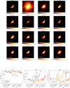 |
Fig. 3 Same as Fig. 2, but for the synthetic loop configuration. |
| In the text | |
|
Fig. 4 Reconstruction results and scoring of the various imaging algorithms on the crescent source model observed with the EHT configuration. The upper panel compares the reconstructions, the lower left panel shows the correlation, the lower middle panel the resolution and the lower right panel the dynamic range. Note: resolution values are close to zeros for a few algorithms (Cons_MEM, MEM, l1 and MEM_l1) since they over-resolve the source, namely, they recover structures that are finer than those in the ground truth image due to too much enhancing of the regularizer. |
| In the text | |
|
Fig. 5 Reconstruction results and scoring of the various imaging algorithms on the GRMHD source model observed with the ngEHT configuration. The upper panel compares the reconstructions, the lower left panel shows the correlation, the lower middle panel the resolution and the lower right panel the dynamic range. |
| In the text | |
|
Fig. 6 Comparison of the reconstruction quality among different CLEAN variants (CLEAN, U-CLEAN, Clean with uniform weights, and DoB-CLEAN), benchmarked against bayesian reconstructions and reconstructions done with MEM_GE, in the case of the STIX double Gaussian configuration. The lower left panel shows the correlation, the lower middle panel the resolution and the lower right panel the dynamic range. |
| In the text | |
|
Fig. 7 Imaging results of SOL2023-05-16T17 event recovered with various algorithms (CLEAN, U-CLEAN, MEM_GE, resolve, and DoG-HiT, from left to right, respectively). |
| In the text | |
Current usage metrics show cumulative count of Article Views (full-text article views including HTML views, PDF and ePub downloads, according to the available data) and Abstracts Views on Vision4Press platform.
Data correspond to usage on the plateform after 2015. The current usage metrics is available 48-96 hours after online publication and is updated daily on week days.
Initial download of the metrics may take a while.