| Issue |
A&A
Volume 692, December 2024
|
|
|---|---|---|
| Article Number | A255 | |
| Number of page(s) | 14 | |
| Section | Galactic structure, stellar clusters and populations | |
| DOI | https://doi.org/10.1051/0004-6361/202449255 | |
| Published online | 17 December 2024 | |
3D structure of the Milky Way out to 10 kpc from the Sun
Catalogue of large molecular clouds in the Galactic Plane
1
Max-Planck-Institute for Astronomy,
Königstuhl 17,
69117
Heidelberg,
Germany
2
Chalmers University of Technology, Department of Space, Earth and Environment,
412 93
Gothenburg,
Sweden
3
Department of Physics, University of Wisconsin-Whitewater,
Whitewater,
WI
53190,
USA
4
Physics Department and Kavli Institute for Astrophysics and Space Research, Massachusetts Institute of Technology,
77 Massachusetts Ave,
Cambridge
MA
02139,
USA
5
Laboratoire de Physique de l’École Normale Supérieure, ENS, Université PSL, CNRS, Sorbonne Université, Université de Paris,
75005
Paris,
France
6
Observatorio Astronómico Nacional (IGN),
C/Alfonso XII 3,
28014
Madrid,
Spain
7
Centro de Desarrollos Tecnológicos, Observatorio de Yebes (IGN),
19141
Yebes, Guadalajara,
Spain
★ Corresponding author; This email address is being protected from spambots. You need JavaScript enabled to view it.
Received:
17
January
2024
Accepted:
24
October
2024
Abstract
Understanding the 3D structure of the Milky Way is a crucial step in deriving properties of the star-forming regions, as well as the Galaxy as a whole. We present a novel 3D map of the Milky Way plane that extends to 10 kpc distance from the Sun. We leverage the wealth of information in the near-infrared dataset of the Sloan Digital Sky Survey’s Apache Point Observatory Galactic Evolution Experiment (APOGEE) and combine that with our state-of-the-art 3D mapping technique using Bayesian statistics and the Gaussian process to provide a large-scale 3D map of the dust in the Milky Way. Our map stretches across 10 kpc along both the X and Y axes, and 750 pc in the Z direction, perpendicular to the Galactic plane. Our results reveal multi-scale over-densities as well as large cavities in the Galactic plane and shed new light on the Galactic structure and spiral arms. We also provide a catalogue of large molecular clouds identified by our map with accurate distance and volume density estimates. Utilising volume densities derived from this map, we explore mass distribution across various galactocentric radii. A general decline towards the outer Galaxy is observed, followed by local peaks, some aligning with established features such as the molecular ring and segments of the spiral arms. Moreover, this work explores extragalactic observational effects on derived properties of molecular clouds by demonstrating the potential biases arising from column density measurements in inferring properties of these regions, and opens exciting avenues for further exploration and analysis, offering a deeper perspective on the complex processes that shape our galaxy and beyond.
Key words: ISM: clouds / dust, extinction / ISM: structure / Galaxy: disk / Galaxy: structure / galaxies: star formation
© The Authors 2024
 Open Access article, published by EDP Sciences, under the terms of the Creative Commons Attribution License (https://creativecommons.org/licenses/by/4.0), which permits unrestricted use, distribution, and reproduction in any medium, provided the original work is properly cited.
This article is published in open access under the Subscribe to Open model.
Open Access funding provided by Max Planck Society.
1 Introduction
The multi-physics, multi-scale nature of star formation is the centre of today’s star formation challenges. Understanding the gathering of material from small scales in protoplanetary discs to molecular clouds and its accumulation in galaxies are key to providing a holistic picture of star formation (Kennicutt & Evans 2012; Padoan et al. 2014; Krumholz et al. 2018).
Star-forming regions contribute to the overall evolution of galaxies, and different galactic environments affect the formation and evolution of star-forming regions. The structures of the Galactic-disc components, such as spiral arms, influence the distribution and evolution of gas and dust, and therefore star formation in a galaxy. Spiral galaxies exhibit active star formation within their spiral arms composed of a concentration of gas and dust. To understand the role of spiral arms in star and galaxy formation and evolution, knowledge of the location of the arms, as well as their components is of utmost value. Using the current observational techniques, resolving individual stars formed within their birth environment and their position within the large-scale galactic environments turns the Milky Way into a unique laboratory. However, our position within the dusty Milky Way disc has long limited our understanding of the location and substructures of the Milky Way star-forming arms to the 2D plane-of-the-sky views and uncertain kinematic distances.
The spiral nature of the Milky Way was initially identified in the 1950s through the determination of distances to objects emitting emission lines and the discovery of 21 cm radio observations (Oort & Muller 1952; van de Hulst et al. 1954; Morgan 1955). Since then, numerous works have focused on characterising the positions of spiral arms in the Milky Way via various approaches, from studying young stars (Russeil 2003; Cantat-Gaudin et al. 2018; Romero-Gómez et al. 2019) to atomic and molecular gas kinematics (Drimmel & Spergel 2001; Kalberla & Kerp 2009; Dame et al. 2001; Roman-Duval et al. 2010; Miville-Deschênes et al. 2017) and maser parallax measurements (Reid et al. 2019). However, despite all improvements, due to challenges in estimating distances and obscuration caused by line-of-sight (LOS) extinction, an accurate picture of the exact structure of our galaxy remains elusive to this date.
Multi-scale 3D maps of the Milky Way are not only important from the Galactic perspective, but they also provide the primary steps required to connect the Galactic and extragalactic star-formation studies. Owing to the new developments in extragalactic observations, recent studies of external galaxies have reached the resolutions of individual large molecular clouds (tens of parsecs; e.g. Schinnerer et al. 2013; Leroy et al. 2021; Sun et al. 2020; Leroy et al. 2021). Kainulainen et al. (2022) showed the substantial effects that the viewing angle can have on the estimated properties of the molecular clouds. A face-on view of the Milky Way taken from the 3D maps further allows us to study the effects of observations on derived star-formation properties of external galaxies; these include observed aperture size, inclinations and viewing angles, and scale height on the obtained physical properties.
Since its launch in 2013, the European Space Agency’s Gaia mission has revolutionised Milky Way studies by providing accurate astrometric measurements to individual sources (Gaia Collaboration 2016). The latest Gaia data release (Gaia DR3) in 2022 contained full astrometric solutions for nearly 1.5 billion sources with a magnitude limit of G=21 (Gaia Collaboration; Brown 2021). The parallax estimates of Gaia with micro-arcsecond precision levels are the main source of recent 3D developments in the Milky Way studies. The Gaia satellite therefore offers an ideal set of data for studying nearby individual molecular cloud substructures in 3D (e.g. Großschedl et al. 2018; Rezaei Kh. et al. 2018a, 2020; Rezaei Kh. & Kainulainen 2022; Zucker et al. 2021), as well as the 3D structure of the local Milky Way (e.g. Green et al. 2019; Leike et al. 2020; Vergely et al. 2022; Edenhofer et al. 2024). Furthermore, the precise 3D positions of a wide range of stellar types observed by Gaia allow the association of stars of different masses and ages with various cloud components in the ISM in order to study the evolutionary stages of molecular clouds (Rezaei Kh. et al. 2020). However, due to the optical nature of the Gaia observations, the studies remain limited to nearby (<∼3 kpc) regions. Therefore, to study the large-scale physics of the ISM, complementary near-infrared (IR) datasets are of great importance. In a pilot study in Rezaei Kh. et al. (2018b), we showed that the strength of the near-IR data makes them great tools for approaching far distances in the Galactic plane. In this work, we showcase the power of near-IR data combined with machine-learning techniques to provide a novel 3D map of our Galaxy that expands out to 10 kpc.
The paper is organised as follows. We briefly summarise our 3D mapping technique and the dataset used in this work in Sect. 2. We then present the 3D map of the Milky Way and explain its features in Sect. 3; this is followed by the catalogue of large molecular clouds from our map. In Sect. 4, we compare our map to existing CO and maser observations and discuss the distribution of the clouds in the Galaxy. Additionally, we discuss our findings in the context of extragalactic studies in Sect. 4.4. The catalogue of selected large molecular clouds and the full 3D map are uploaded online with the paper. Users are advised to read the caveat section before using the full 3D map.
2 Data and methods
In this section, we explain the input data and the technique used for the production of our 3D map.
2.1 3D mapping technique
Our 3D mapping technique was extensively explained in Rezaei Kh. et al. (2017, 2018b), with further changes and improvements explained in Rezaei Kh. et al. (2020). Here, we briefly summarise the main aspects of our 3D analysis. Our technique uses the 3D positions of the stars (l,b,d) and their LOS extinction as the input data. It then divides the LOS of each star into small 1D cells in order to approximate the observed extinction towards each star as the sum of the dust in each cell along its LOS. After having done that for all observed stars, our likelihood is formed. The model then takes into account the neighbouring correlation between all points in 3D using the Gaussian process; that is, the closer two points are in the 3D space, the more correlated they are. This is our prior. Having prepared both the likelihood and the prior, the model uses extensive linear algebraic analysis to determine the probability distribution of dust density at any arbitrary point in the observed space, even along the LOS that was not originally observed.
Our 3D mapping technique consists of the following unique features.
It accounts for both distance and extinction uncertainties in the input data. As a result, our input is not limited to strict data quality cuts and can leverage more observed stars.
Owing to the Gaussian-process-based 3D spatial correlation, the final results are smooth and clear of LOS elongated artefacts, also known as ‘fingers-of-god’ effects.
The predicted dust densities are analytically calculated, thereby minimising biases and artefacts that can arise from the use of Gaussian-process approximations. Consequently, our predictions can be directly traced back to the input data.
Both the mean and standard deviation of the predicted densities are calculated analytically; thus, the precision and reliability of our predictions can be directly evaluated, which increases the robustness of our analysis.
The model incorporates several hyper-parameters determined by the input data (for more details, see Rezaei Kh. et al. 2017, 2018b). One of these parameters is the cell size, which is tuned based on the typical spacing between input stars and serves as the minimum resolution for the final map. In areas with denser and more informative data, the map’s resolution will be higher. Another parameter is the correlation length, which defines the range over which spatial correlations exist. Typically, it is a few times the cell size to ensure the connection between nearby cells in 3D. The third hyperparameter, known as the scale variance, is calculated using the data’s amplitude and uncertainties, reflecting the variance of predictions. After introducing the datasets in the following section, we detail these parameters for our models.
2.2 Input data: Distance and extinction estimates
The Sloan Digital Sky Survey IV’s Apache Point Observatory Galactic Evolution Experiment (APOGEE-2, Blanton et al. 2017; Majewski et al. 2017; Abolfathi et al. 2018) is a near-IR, high- resolution spectroscopic survey targeting bright stars (Eisenstein et al. 2011; Zasowski et al. 2013). In the near IR, the effects of extinction are about an order of magnitude lower than at optical wavelengths, enabling APOGEE to observe stars in the highly obscured regions of the Galactic disc and towards the Galactic centre. APOGEE does not survey the sky uniformly, but rather it targets cool stars, particularly red giants, through multiple components of the Galaxy including thin and thick discs (Eisenstein et al. 2011; Zasowski et al. 2013). The 16th data release of APOGEE published in 2020 (Jönsson et al. 2020), covers different parts of the Galactic plane out to distances beyond the Galactic centre and includes sources from the southern hemisphere (Jönsson et al. 2020). This allows us to map the Milky Way plane with resolutions down to giant molecular cloud sizes (from tens of parsecs to a few hundred parsecs, depending on the APOGEE data coverage) and probe the large-scale structure of the Galaxy (such as spiral arms) and the properties of the large molecular clouds to unprecedented accuracies to date.
Extinction measurements come directly from the APOGEE pipeline: all APOGEE sources have corresponding observations in multi-band photometry in the near- and mid-IR with the Two Micron All-Sky Survey (2MASS, Skrutskie et al. 2006) and the Wide-Field Infrared Survey Explorer (WISE; Wright et al. 2010), respectively. Therefore, their extinctions are easily estimated using the Rayleigh-Jeans Colour Excess (RJCE; Majewski et al. 2011) method. We did not apply an explicit quality cut on the APOGEE data. Instead, after calculating the extinctions, we removed data with unrealistic extinction values, which may occur due to a star’s variability or circumstellar dust (for further details, please refer to Rezaei Kh. et al. 2018a, 2020).
As mentioned in Sect. 2.1, in order to infer the 3D distribution of the dust, our method requires the 3D positions of stars. The distance estimates for the APOGEE sources are calculated using spectrophotometric parallaxes computed based on the method of Hogg et al. (2019). The approach leverages a data-driven model that combines photometric and spectroscopic data, aiming to describe the parallaxes of giant stars. It employs a feature vector containing photometric and spectroscopic information, resulting in a 7460-dimensional feature space. The optimisation process considers the uncertainties in Gaia parallax measurements, and an offset is applied to account for known parallax biases. Given the sparsity of information within APOGEE spectral pixels, a regularisation term is introduced to enhance the model’s accuracy. The study achieves a median relative uncertainty in spectrophotometric parallax of ~8%, which is a significant improvement compared to the Gaia parallax, especially for stars beyond a heliocentric distance of 3 kpc (Hogg et al. 2019; Ou et al. 2024). For a more comprehensive understanding, readers are encouraged to refer to the original paper. This enhanced accuracy enables the mapping of the Milky Way up to distances beyond the Galactic centre.
Having obtained distance and extinction estimates, we have all the essential input data needed for our model. Given our specific interest in the structure of the Galactic lane and considering that the majority of APOGEE observations are designed for these regions, we narrow down our input data to include only absolute Galactic heights below 1 kpc, allowing us to focus on the Milky Way midplane. Figure 1 shows the input data used in our model. While the distance estimates for APOGEE sources extend beyond 10 kpc of the sun, the density distribution of stars, as illustrated in Fig.1, notably decreases as we approach the 10 kpc distance. As a result, we confine our map to the 10 kpc range along the X- and Y -axes. The final sample contains more than 44 000 stars, and the maximum K-bank extinction in the sample is ~ 1.6 magnitudes. We also note that the number of stars drops significantly in the inner ~500 pc; therefore, we limit our predictions to distances beyond 1 kpc.
As mentioned in Sect. 2.1, the hyper-parameters of the model are set according to the input data. For the APOGEE data used in this work, the parameters are as follows: cell size of 200 pc, correlation length of 1 kpc, and scale variance of 5 × 10⁻⁹ pc−2. Additionally, for all plots and analysis in this work, we assume a distance between the Sun and the Galactic centre of 8.2 kpc and a height from the Galactic midplane of 7 pc (in agreement with Reid et al. 2019; GRAVITY Collaboration 2021; Darling et al. 2023; Leung et al. 2023).
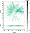 |
Fig. 1 Final sample used as our input data. The top panel shows the X-Y plane, which is perpendicular to the Galactic plane, and the bottom panel presents the X − Z plane where our cut on the 1 kpc Galactic height is visible. The colour shows estimated extinctions for individual stars. The Sun is at (−8.2,0,0) and the Galactic centre is marked with an X, assuming the Sun is at the distance of 8.2 kpc from the Galactic centre. The gaps between different LOSs indicate that the sky is not observed uniformly by APOGEE. |
3 Results
Using the input data (as explained in Sect. 2), we produce the 3D map of the dust in the Galactic plane for a radius of 10 kpc in the X − Y plane and 750 pc in the Z direction, perpendicularly to the Galactic plane. Our predictions are made for points on a regular grid of 100 pc in X and Y and for five layers in the Galactic heights of −750, −375, 0, 375, and 750 pc. Given the sparsity of the APOGEE data, which sets the model’s hyper-parameters, especially in regions away from the Galactic midplane, predicting on a denser grid in either X, Y, and Z directions does not add further useful information to the map.
3.1 Features of the map
Figure 2 shows our 3D map for different Galactic heights, as well as a combined map. The white areas are regions devoid of input stars; this is particularly visible in parts of the fourth quadrant of the Galactic midplane (Z=0) where, as seen in Fig. 1, our current input lacks data. The densities are converted from our model’s units of mag/pc to cm−3 assuming AK/NH = 0.7 × 10⁻²² cm2 mag/H Draine (2009). Numerous dust density substructures are visible in Fig. 2 at various distances and heights, the majority of which appear, as expected, in the Galactic midplane (z=0). In particular, there are multiple high-density clouds towards the Galactic centre, with the densest structures of the map appearing at a galactocentric radius of about 4 kpc, that are likely associated with the so-called molecular ring (Krumholz & McKee 2005). We do not see major differences between positive and negative heights in terms of the presence of the warp in the Galaxy. This could be due to the incompleteness in the range covered by the input data, or the presence of the stellar warp in further distances, as suggested by Poggio et al. (2020).
As explained extensively in our previous works (Rezaei Kh. et al. 2017, 2018b, 2020) and in Sect. 2.1, the robustness of the 3D dust maps, especially those based on Gaussian processes, lies within the reliable calculation of the uncertainties. Therefore, we use our predicted mean densities together with their uncertainties, which are calculated analytically. The left panel of Fig. 3 shows our 3D map with shaded areas representing regions of large uncertainties (fractional uncertainties larger than 50%). A separate uncertainty map is also shown in Appendix A. The smallest fractional uncertainty is about 5% and belongs to high- density regions. The radial patterns in the shaded plot clearly show areas with a lack of input data, as seen in Fig. 1.
The right panel of Fig. 3 shows clouds extracted from the 3D map with statistically significant densities. Statistically significant in this context means three standard deviations above the mean of the Gaussian process that is used for density calculations. It is important to note that this does not imply three sigma above the ‘noise’, which in this case would be around zero, but refers to a much higher threshold: the Gaussian process uses a mean density for each region based on the input stellar extinction, which is already higher than the average noise. In order to make sure the clouds are ‘real’ and their densities are not derived by the mean density of the Gaussian process, we go three standard deviations above this value to have a pure sample of dense clouds. This corresponds to densities above ~80 cm−3. The fractional uncertainties of the selected clouds are between 5 and 30%. The first evaluation of the map and the clouds within it does not show a clear indication of the spiral arms in the Milky Way. The Local Arm and segments of the Perseus Arm are the only clear arm features that could be extracted from the map. We explore these further in Sect. 4.
From our map of clouds (Fig. 3, right), we select regions with densities above 100 cm−3, corresponding to the molecular phase, and provide a catalogue of large molecular clouds in the Milky Way (Table A.1). We deliver accurate distance estimates to the centre of each cloud, the uncertainty of the estimated distance, the extent of the cloud, its mean density and standard deviations, and its association with known star-forming regions and spiral arms.
The associations with spiral arms and star-forming regions have been determined using a combination of catalogues and studies; in the first quadrant, we used the catalogue of molecular clouds from Dame et al. (1986), which has a similar resolution to our map, combined with the BESSEL distance calculator (Reid et al. 2016). The BESSEL survey uses a combination of maser parallaxes, spiral arm models based on masers, and kinematic distances to give all probable distance estimates for a given LOS and velocity (l,b,v). For each cloud from Dame et al. (1986) with a matching LOS to a cloud centre from our map, we use the BESSEL distance calculator to obtain all probable distance estimates for that (l,b,v). For a given LOS, if we had a peak in density in our 3D map (within 0.5 degrees from that LOS) that matches one of the probable distance estimates from the BESSEL survey for that (l,b,v), we assume they correspond to one another (see Fig. 4 for an example). For the rest of the map, we use the catalogue of radio sources from Westerhout (1958) associated with star-forming regions, the catalogue of Hα-emission regions in the southern Milky Way by Rodgers et al. (1960), and the catalogue of star-forming regions by Binder & Povich (2018). For the arm associations, we used masers from Reid et al. (2019).
In addition to the over-densities and spiral arm segments, one clear feature of the map is the presence of large cavities. These cavities are visually identified as regions of low-density surrounded by higher densities and marked by dashed lines in Fig. 5. While we were able to extract a clear sample of clouds with reliable densities from the map, distinguishing real cavities from regions of underestimated densities due to missing data remains difficult. The peak of the stellar density as a function of distance gradually declines after 5 kpc; as a result, given our 1 kpc correlation length, we limit our sample of the cavities to nearby regions (within ∼4 kpc of the Sun) to avoid mistakenly categorising regions without complete input data as cavities. This would also allow comparison to other 3D maps with overlapping regions. We also avoid selecting cavities in the southern hemisphere altogether due to incomplete data.
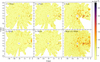 |
Fig. 2 Frontal view of our 3D map of dust in Galactic plane for different Galactic heights. The bottom right panel shows the combined map from -750 pc to 750 pc in the Galactic height. The colour shows the mean of our predicted density (cm−3) for each pixel (100×100 in X − Y plane) in all panels, except for the bottom right where the colour represents the maximum density within the 1.5 kpc height. The Sun is at (−8.2,0,0) and the Galactic centre is marked with an ×, assuming the Sun is 8.2 kpc from the Galactic centre. White regions are areas devoid of input data. |
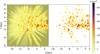 |
Fig. 3 Frontal view of 3D map for all Galactic heights. Left panel: same as bottom right panel of Fig. 2, in addition to having shaded areas illustrating regions of high uncertainty (fractional uncertainties larger than 50%). Right panel: clouds selected from 3D map whose density values lie three standard deviations above the mean of the Gaussian process. This corresponds to densities above 80 cm−3. |
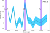 |
Fig. 4 Example of how clouds in Table A.1 are assigned to known structures and spiral arms. The black line with the blue shaded uncertainties are our density predictions as a function of distance for a given LOS, and the purple vertical lines are all probable distance estimates from the BESSEL survey (Reid et al. 2016) for the same LOS with velocities observed in Dame et al. (1986) (e.g. Aquila rift, Sagittarius Near, and Perseus here). The dashed red line indicates our threshold for selecting statistically significant clouds. If there is a match, such as the near Sagittarius Arm in the middle, we assign the cloud to that particular structure. The LOS’ galactic longitude and latitude are shown in the top right corner. |
3.2 Comparison to other 3D maps
Vergely et al. (2022) provided one of the most promising maps of the Galaxy by combining Gaia parallaxes with the crossmatching of the Gaia data with 2MASS and WISE photometry. They also considered a full 3D correlation in space to provide an artefact-free, smooth 3D map of the Milky Way out to 4.5 kpc from the Sun at a resolution of 25 pc (Vergely et al. 2022). Green et al. (2019) used multi-band photometry from PANSTARRS together with the Gaia parallaxes to simultaneously derive distance and extinction to individual stars. Their map has a high resolution on the plane of the sky; however, due to the separate treatment of each LOS, elongated artefacts are visible in their final map. The technique of Marshall et al. (2006) is particularly different to the others: they measure the colour excess of stars by assuming a Galaxy model and the intrinsic colours of stars. They then use this colour excess to determine a star’s distance and extinction. While there are substantial LOS elongations in the map of Marshall et al. (2006), it is the only one that reaches similar distances to that of our map towards the inner Galaxy.
Figure 5 shows a qualitative comparison between our map and three other maps each based on different techniques and datasets. The maps also show various resolutions, features, artefacts, and density ranges. As a result, we limit our comparison to dominant features and structures of the maps and avoid quantitative comparisons. Large cavities in our map are marked by dashed lines. While a direct comparison to Marshall et al. (2006) and Green et al. (2019) maps seem difficult because of the existing artefacts, there are still noteworthy features to consider: the large cavity marked in the first quadrant of our map is clearly visible in the map of Marshall et al. (2006), together with its surrounding over-densities. The cavity in the third quadrant and the over-densities adjacent to its left are also visible in Green et al. (2019). Amongst all maps, the one from Vergely et al. (2022) shows the most promising comparison. All four large cavities discovered in our map are clearly visible in Vergely et al. (2022), as are most of their surrounding over-densities. While our map and that of Vergely et al. (2022) are in good qualitative agreement, there are some differences as well: our map has a much larger distance coverage, and in return the resolution of Vergely et al. (2022) is on average four times better than ours; as a result, they recover much smaller structures than our map can achieve.
This is visible, for instance, at l = 270°, where our map recovers a large over-density around the location of the Vela molecular cloud ((x, y) = (−8, −2) kpc), while around the same region, Vergely et al. (2022) recovers multiple smaller substructures that our map is not able to resolve.
Another significant aspect of our map involves multiple overdensities observed towards the Galactic centre (Y ≃ 0). The most prominent dense clouds manifest at galactocentric radii of around 3 and 4 kpc. Additionally, there are several overdensities in this direction at galactocentric radii of 4.5 and 6 kpc. While Vergely et al. (2022) showed numerous smaller clouds in this direction, one particular cloud at galactocentric radii of about 4.5 kpc appears to align with ours. However, as Vergely et al. (2022) noted, the reliability range of their map towards the inner Galaxy is particularly limited up to about 4 kpc from the Sun. Conversely, the map of Marshall et al. (2006) map offers extensive coverage for comparison in direction of the inner Galaxy. Multiple over-densities are visible in Marshall et al. (2006) towards the direction of the Galactic centre. Two dense regions around X = −3, one on the Y = 0 line and another slightly below it, correspond well with our dominant clouds in that region, although at slightly different distances. Similarly, another over-density in their map at X ≃ −4.5, just above the Y = 0 line, corresponds well with ours. Additionally, some clouds identified in the first quadrant of our map align with those in Marshall et al. (2006), although differences in distances are observed due to uncertainties and elongated radial structures in Marshall et al. (2006). While our map remains relatively incomplete in most of the fourth quadrant, a few recovered clouds seem to correlate with those in the map of Marshall et al. (2006) as well.
A notable difference between Marshall et al. (2006) and our map lies in the density distribution around the Galactic centre. While Marshall et al. (2006) reveals a cavity around and below the Galactic centre, our map depicts a few clouds in that vicinity. Understanding the reasons for these differences presents a challenge, but we offer our insights on the subject here. As seen in the bottom panel of Fig. 1, our input data reveal incompleteness around the Galactic centre at b = 0. Consequently, most of the identified over-densities in our map around this area stem from adjacent data at higher or lower latitudes. While we acknowledge data incompleteness around the Galactic centre, we anticipate that with a more comprehensive dataset covering this region we would identify more clouds and denser concentrations, rather than the reverse. This is supported by recent studies towards the Galactic centre and the central molecular zone (CMZ), where an accumulation of molecular gas is observed (for an overview of the CMZ, see Henshaw et al. 2023). The observed under-density in Marshall et al. (2006) could similarly result from incomplete data in that region or inaccurate distance estimations for stars due to crowding and confusion. The forthcoming data from SDSS-V (Kollmeier et al. 2017) may well shed light on this matter.
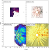 |
Fig. 5 Comparison of locations of high-density dust in 3D dust maps of Galactic plane. Grids are drawn for easier comparisons between maps. The lower right panel shows our 3D map where dashed lines represent identified large cavities. Similar cavities are seen in the upper right panel representing the work of Vergely et al. (2022). While matching cavities seem to be present at similar locations in the other two panels, (Green et al. 2019; Marshall et al. 2006), due to substantial artefacts a direct comparison appears difficult. Apart from our map, only the work of Marshall et al. (2006) expands beyond the Galactic centre; despite the elongated artefacts, multiple over-densities in the first quadrant and towards the Galactic centre are evident on both maps. The range and the width of the maps along the Z direction vary; Vergely et al. (2022) covered from Z=−400 pc to Z=400 pc and provides extinction densities ranging between 0 and 5 × 10⁻³ mag/pc, while Green et al. (2019) covered Z=−300 pc to Z=300 pc and provides differential extinction ranging from 0 to 0.5 mag/kpc. Marshall et al. (2006) covered |b| ≤ 0.25 and represents average extinction density of 0–0.4 kpc−1. |
4 Discussion
In this section, we discuss our results in the context of Galactic structure and radio observations, as well as its application in extragalactic studies.
4.1 Milky Way structure and masers
We first compare our results with the locations of high-mass starforming regions identified by trigonometric parallaxes of maser emissions (Reid et al. 2019). Mapping the spiral structure of the Milky Way poses significant challenges due to vast distances and dust obscuring the Galactic plane in optical wavelengths. However, using Very Long Baseline interferometry (VLBI) in radio wavelengths, unaffected by dust, has proven effective in identifying molecular masers linked to young massive stars, providing valuable insights into spiral structures (Reid et al. 2019). Reid et al. (2019) conducted a comprehensive analysis, gathering around 200 trigonometric parallaxes and proper motions of these masers, primarily from the BeSSeL survey through the VLBA and Japanese VERA project. They associated observed masers with spiral arms by considering patterns in CO and HI Galactic longitude–velocity plots, alongside Galactic latitude information, enabling a better understanding of the Milky Way’s spiral structure.
Figure 6 shows masers from Reid et al. (2019) over-plotted on our clouds extracted from the 3D map (see Sect. 3.1 and Fig. 3). There is a significant overlap between our clouds and the masers, particularly at the location of the Local Arm, segments of the Perseus Arm, as well as the Sagittarius–Carina arm. There are several clouds underneath masers belonging to Scutum–Centaurus–OSC, the Norma arm, and the spurs in the inner Galaxy; however, it is difficult to establish a one-to-one relation due to the crowding in both masers and cloud distributions. Regardless, the multiple over-densities towards the Galactic centre identified in our map (see Sect. 3.2) are well represented by the masers in Reid et al. (2019). Additionally, while there seems to be an offset between the masers and our clouds at the location of the Outer Arm in the outer Galaxy (red points), our clouds seem to turn and follow the potential spiral arm pattern. This could suggest that the clouds and masers represent different parts of the same spiral arm.
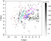 |
Fig. 6 Grey scale showing clouds extracted from our 3D dust map (same as Fig. 3, right). The colour-coding follows the same as Fig. 1 in Reid et al. (2019). Each colour represents masers belonging to a spiral arm as follows: 3-kpc arm: yellow – Norma–Outer arm: red – Scutum–Centaurus–OSC arm: blue – Sagittarius–Carina arm: purple – Local arm: cyan – Perseus arm: black. The Green points are equivalent to the white points in Reid et al. (2019), illustrating spurs or sources with unclear arm associations. |
4.2 Comparison to CO
Miville-Deschênes et al. (2017) provided a catalogue of 8107 molecular clouds spanning the entire Galactic plane and containing 98% of the observed 12CO emission within a latitude range of ±5 degrees. The catalogue was produced using a hierarchical cluster identification technique applied to the Gaussian decomposition of data initially compiled by Dame et al. (2001). They estimated distances to the clouds using kinematic distance estimates following Roman-Duval et al. (2009) and the rotation curve defined in Brand & Blitz (1993). They provide physical properties of the clouds including, but not limited to, 3D positions, surface density, physical size, and mass (Miville-Deschênes et al. 2017).
We compare our results to their cloud distribution in Fig. 7. We first over-plot our clouds as contours on their molecular cloud distribution on the face-on view of the Galaxy. There is a wide circular void in the CO clouds of Miville-Deschênes et al. (2017), which are particularly noticeable around the Galactic centre, extending for about 4 kpc, which is due to limitations in the kinematic distance estimates at these regions. There is a good agreement between our cloud locations and the CO clouds around the position of the Local Arm. However, as we get closer to the inner Galaxy and near the Galactic centre, it once again becomes difficult to conclude due to the crowding. It is also important to note that because of the kinematic distance estimates for the CO sources, the distance uncertainties become quite significant in the crowded inner Galaxy (far away), in addition to the possible near and far confusion.
Nevertheless, we proceeded with our comparison by extracting CO clouds situated at the same position as our clouds in Fig. 7, left, utilising their velocity information to construct a longitude–velocity (L−V) diagram. In Fig. 7, right, presence patterns on the L−V diagram are typically indicative of spiral arms and are commonly used to develop and validate arm models (e.g. Reid et al. 2019). The presence of circular motions for the selected molecular clouds is evident from the loop-like trails. Conversely, no clear arm pattern emerges in Fig. 7, left, and modelling spiral features from the L−V diagram in Fig. 7, right, poses considerable challenges due to the unclear and incomplete arrangement of the molecular clouds.
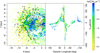 |
Fig. 7 Comparison between our clouds and molecular clouds observed in CO. Left panel: 3D distribution of molecular clouds observed in CO from Miville-Deschênes et al. (2017), with our extracted clouds over-plotted as contours. Right panel: longitude-velocity plot of molecular clouds from the left, situated underneath our cloud contours. The colour shows the surface density of clouds derived in Miville-Deschênes et al. (2017). |
4.3 Mass distribution in the Galaxy
Having the 3D distribution of the clouds in the Galactic plane allows the study of the mass distribution as a function of the galactocentric radius. Figure 8 shows the total mass as a function of the galactocentric radius for rings of 1 kpc thickness around the Galactic centre; this is derived from our 3D dust volumedensity map and that of Miville-Deschênes et al. (2017). To have a fair comparison, we removed clouds from Miville-Deschênes et al. (2017), where our map is unable to recover clouds (e.g. parts of the fourth quadrant or at distances beyond the Galactic centre). For the inner 2 kpc, our map covers the full circle while calculating the mass for the radial bins; however, the outer regions are only averaged over half of a circle (negative X in the previous plots) because of our limited coverage. It is important to note that due to the lack of data in the Galactic plane within the inner 4 kpc galactocentric radii (see Fig. 1, bottom), we underestimate the total mass in these regions (marked by shaded areas in Fig. 8, top).
Overall, the total mass decreases as a function of galacto- centric radius, followed by several local peaks. This has already been observed in other studies (e.g. Elia et al. 2022; Miville-Deschênes et al. 2017; Lee et al. 2016; Kennicutt & Evans 2012); however, the location of the peaks in different studies is not always consistent. We find the first peak at about 4 kpc, likely associated with the molecular ring; this was predicted by Krumholz & McKee (2005). The peak was reported by Chiappini et al. (2001) at 4 kpc, Miville-Deschênes et al. (2017) at 4.5 kpc, and Elia et al. (2022) at 5 kpc. However, as mentioned earlier, our results within the galactocentric radii of 4 kpc should be treated with caution due to incomplete input data in the inner Galaxy. It is also important to note that the dip between 1 and 4 kpc in Miville-Deschênes et al. (2017) (Fig. 8, bottom), and similar works relying on kinematic distances, is not a real effect but due to the lack of data in these regions, as illustrated in Fig. 7 and Sect. 4.2. Additionally, we see a local dip between 4 and 5 kpc followed by a secondary peak at 6.5 kpc, which is in agreement with the 6 kpc peaks of Miville-Deschênes et al. (2017); Elia et al. (2017). The 6.5 kpc peak matches the location of the near Sagittarius–Carina arm (see Fig. 6). One of the most prominent peaks in Fig. 8 is the local peak at 8.5 kpc. This matches very well with the local peak of Miville-Deschênes et al. (2017) and could be the result of the arrangement of clouds at the Local Arm and a large segment of the fourth quadrant (see Fig. 7, left). There are slight increases at further distances of about 10.5 and 12.5 which could potentially be derived from the concentration of clouds in a segment of the Perseus Arm and the Outer Arm at these distances; however, the peaks are not as prominent as the previous ones.
A significant difference between the two works is the derived mass values. This difference can be investigated in various directions: differences in the data used in each work (stellar extinctions vs. CO emission observations), the depth and coverage of these data, and the conversion factors used to translate extinction into density and CO into molecular hydrogen mass. Further analysis is required to thoroughly explore the underlying reasons.
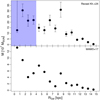 |
Fig. 8 Mass as function of galactocentric radius for clouds from our 3D map (top) and CO from Miville-Deschênes et al. (2017) (bottom) for galactocentric rings of 1 kpc thickness. In this plot, we exclude CO clouds from Miville-Deschênes et al. (2017) belonging to regions not covered by our map (e.g. parts of the fourth quadrant). The shaded area shows regions where our results are likely underestimated due to the lack of input data. We did not limit the azimuth range for each radial bin; however, due to the limitations in the map, for regions beyond a galactocentric radius of 2 kpc, our radial average only covers half of a circle (negative X in previous figures). |
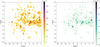 |
Fig. 9 Comparison of volume density and column density. Left panel: volume densities of clouds from our 3D map (same as Fig. 3, right). Right panel: column densities of left side clouds integrated over the Z access. |
4.4 Impact on extragalactic studies
Recent years have seen a surge in studies examining molecular clouds in other galaxies, leveraging our knowledge from the Milky Way to a diversity of extragalactic environments (e.g. Kawamura et al. 2009; Donovan Meyer et al. 2013; Schinnerer et al. 2013; Freeman et al. 2017; Lee et al. 2023). Large surveys such as PHANGS–ALMA (Leroy et al. 2021) allow us to analyse high-sensitivity and -resolution observations of giant molecular clouds (∼60–150 pc) across nearby, massive, star-forming galaxies. Understanding the relationship between these clouds and their galactic surroundings is vital in order to grasp the underlying physics governing their evolution (Sun et al. 2022).
All these observations, however, rely on observed integrated intensities to define and identify discrete molecular clouds and, therefore, can be subject to the projection effects. Observing molecular clouds at large distances increases the probability of having an overlap of different clouds in the same LOS which, in turn, increases the mean column density of the ensemble substantially. Overlapping clouds in the same line of sight, especially in arm regions, contribute to observed scatter in mass–size relations (Colombo et al. 2014; Ballesteros-Paredes et al. 2019).
Using our 3D map, we can view the Milky Way as an external galaxy and estimate some of the observable parameters of extragalactic studies. Figure 9 shows the Milky Way from an external viewpoint with two measured parameters: volume density, not directly accessible to extragalactic astronomy; and column density, widely used in extragalactic studies to infer properties of the star-forming regions and galaxies. The right panel of Fig. 9 is derived by integrating our 3D map (left panel) along the Z axis (i.e. the Galactic height). Notably, Fig. 9 indicates that there is not always a direct correspondence between volume densities (which are directly connected to the physical properties of the clouds) and observed column densities. This occurs due to the buildup of low to moderate densities along the line of sight, creating the illusion of a high-density cloud. This discrepancy holds significant implications for extragalactic studies, particularly when comparing cloud properties across different environments and between galaxies. It not only impacts the location of massive star-forming regions in a galaxy, it also affects the total mass derived for each cloud (see Fig. 9, right, and refer to Rezaei Kh. & Kainulainen 2022; Kainulainen et al. 2022; Cahlon et al. 2024, for further discussion on the projection effects and mass derivation.)
The rotational transitions of CO have been the most popular tracers of the bulk molecular ISM in the Milky Way and other galaxies (e.g. Bally et al. 1987; Dame et al. 2001; Kuno et al. 2007). However, CO is quickly thermalised, so its emission does not reflect the different density regimes of a cloud. Constraining the density distribution of star-forming gas in external galaxies is even more challenging since compact, high- density regions within molecular clouds are hard to resolve. High-critical-density spectroscopic lines such as HCN(1–0) and HCO+ (1–0) have become common tracers of dense gas in galaxy discs. Over the last decade, multiple extragalactic surveys at low (e.g. the EMPIRE survey, Jiménez-Donaire et al. 2019) and high resolution (e.g., Gallagher et al. 2018; Querejeta et al. 2019; Bešlic et al. 2021) have found systematic trends for the star formation efficiency per unit of dense gas as a function of the host galaxy and local environment properties. Nevertheless, these conclusions rest on the ability to translate extragalactic HCN emission into a dense molecular gas mass. In that context, numerous research works have recently shown that these tracers are not as selective of dense gas as previously assumed. Instead, their integrated intensity is dominated by the emission of low-density regions (e.g. Kauffmann et al. 2017; Pety et al. 2017; Evans et al. 2020; Tafalla et al. 2021, 2023; Dame & Lada 2023).
Given the findings of our present study and other Galactic and extragalactic works that concentrate on the LOS superposition effects of multiple clouds and extended objects, affecting the derived properties of the clouds (e.g. Ballesteros-Paredes et al. 2019; Rezaei Kh. & Kainulainen 2022; Kainulainen et al. 2022), one way to minimise such biases involves observations of molecular line emissions in critical high-density environments. In the Milky Way, combining such observations with Galactic rotation curve information helps to distinguish multiple clouds along the LOS based on their high-resolution velocity information. In external galaxies, however, the problem appears more complex. Cloud superposition occurs on various scales (e.g. cores, fibers) and resolutions and along the galactic heights (Ballesteros-Paredes et al. 2019). Even though high-critical-density line observations in external galaxies alone cannot resolve the issue of cloud superposition, they can mitigate the problem by ensuring that the emission originates from high-density regions rather than the accumulation of low densities along the LOS. Such observations have been recently conducted by Jiménez-Donaire et al. (2023) who presented the first systematic extragalactic observations of N2H+(1–0) and HCN(1–0) in a wide range of dynamical conditions and star formation properties sampled across an entire galaxy disc.
It is beyond the scope of this paper to quantify biases in extragalactic studies, as it demands a more comprehensive analysis of involved factors. However, it is evident that properties derived solely from observed column densities carry potential biases, especially with recent advancements in extragalactic observations that capture individual cloud sizes (e.g. Schinnerer et al. 2013; Faesi et al. 2018; Leroy et al. 2021; Sun et al. 2020).
4.5 Caveats
Despite its great potential and strengths, it is crucial to acknowledge the limitations of our study that require consideration. These aspects offer insights into the boundaries and potential constraints of our findings.
As mentioned earlier, one of the main limiting factors in our work lies within the input data. Given the observed patterns of APOGEE, the space is not uniformly observed. There are various gaps in the data both in the local neighbourhood and further outside. As a result, our map underestimates the dust distribution in some regions, the total number of clouds, and, therefore, the total dust mass of the Galaxy. This particularly affects the fourth quadrant and the area near the Galactic centre at b=0, both of which are observed very sparsely.
The final resolution is another limitation imposed on our results due to the incomplete input data. As explained in Sect. 2, the typical separation between the input stars sets the cell size for our model and affects the final resolution of the map. Therefore, given the sparsity in the observed APOGEE data, our final resolution varies from tens of parsecs to a few hundred parsecs, depending on the region. This affects the clouds reported in our catalogue. Our map is unable to resolve multiple small clouds that appear in close vicinity of one another; thus, some of our large clouds could contain unresolved substructures at various distances and densities within the cloud range. An example of this is around the Vela molecular cloud at X = −8 kpc, Y = −2 kpc, which includes multiple clouds in the map of Vergely et al. (2022), with better resolution but limited distances.
Another possible constraint of our work is in the clouds selected from our map for further analyses (Fig. 3, left). To avoid biases, we applied a strict cut-off when selecting clouds from our map (see Sect. 3.1). This results in missing potential low- to mid-density clouds that have values below or around three sigma above the mean of the Gaussian process. Therefore, the selected clouds in our map are incomplete for low to mid densities.
Apart from the catalogue of large molecular clouds in the Milky Way, which is carefully selected, we have also included our 3D density predictions with this publication. Users are, however, advised to take care when working with the map and to only employ its predicted uncertainty to avoid biases and noisy outputs.
5 Concluding remarks
We present the most extended 3D dust map of the Milky Way to date and provide a catalogue of large molecular clouds in the Milky Way. The cloud properties in the catalogue are derived from the 3D map and avoid biases involved in plane-of-the-sky works. The catalogue delivers (non-kinematic) accurate distance estimates to high-density regains and contains their volume densities. Our map illustrates large cavities in the Galactic plane, posing as potential targets for further studies and analysis.
Our 3D map sheds light on segments of the spiral arms; however, we do not observe clear arm patterns in our results. Using the volume densities derived from our map, we also studied the distribution of mass for different galactocentric radii. We observe an overall decreasing trend as we approach the outer Galaxy, followed by multiple local peaks linked to known regions, such as the molecular ring, and segments of the spiral arms.
Additionally, our results provide insights into the extragalactic studies that focus on deriving properties of the clouds in star-forming regions. We demonstrate how the inferred properties of star-forming regions could be biased by using column density measurements, and suggest observations of molecular line emissions in critical high-density environments to minimise such biases. Further studies are required to quantify these biases.
The future of the 3D structure of the Milky Way relies on a uniform, near-infrared survey that covers the entire Galactic plane. This will soon be achieved by the upcoming SDSS-V data (Kollmeier et al. 2017), which follows the legacy of APOGEE and is poised to achieve this ambitious goal.
Data availability
The catalogue of selected large molecular clouds and the full 3D map is available at the CDS via anonymous ftp to cdsarc.cds.unistra.fr (130.79.128.5) or via https://cdsarc.cds.unistra.fr/viz-bin/cat/J/A+A/692/A255
Acknowledgements
The authors acknowledge Interstellar Institute’s program “II6” and the Paris-Saclay University’s Institut Pascal for hosting discussions that nourished the development of the ideas behind this work.
Appendix A Catalogue of large molecular clouds in the Galactic Plane
Catalogue of large molecular clouds in the Galactic plane.
The columns are: cloud ID, Galactic coordinates of the centre of the cloud, distance to the centre of the cloud from the Sun, one sigma distance uncertainty of the centre of the cloud, mean radius and mean density of the cloud, standard deviation from the mean density, and corresponding known associations for the clouds. A cloud with a mean radius/density of NA indicates that only one pixel of the cloud has densities above the molecular threshold of 100 cm−3 ; therefore, it is too small for our map to resolve its size. The standard deviations are sample standard deviations weighted by the predicted standard deviation of the posterior.
The associations with spiral arms and known clouds are determined in multiple ways as follows:
Associated with spiral arms using masers in Reid et al. (2019)
Having a corresponding cloud in Dame et al. (1986), as explained in section 3.1 and Fig. 4
Having a corresponding cloud in Westerhout (1958), Rodgers et al. (1960), or Binder & Povich (2018)
Appendix B Input data
Figure B.1 shows the plane of the sky stellar distribution used as our input data (see also Fig. 1). The pattern is due to APOGEE’s selective pointing observations. Most stars are observed in the Galactic plane with a few at the upper latitudes.
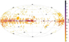 |
Fig. B.1 An aitoff view of the input data representing the pointing pattern of the APOGEE. Most of the data is concentrated in the Galactic Plane, and the Northern Hemisphere with few observations in the Southern Hemisphere as well. colour represents the mean extinction per pixel. |
Appendix C Predicted uncertainties
Figure C.1 shows our predicted uncertainties on the plane of the sky. A lack of input data from APOGEE causes the radial pattern. The fractional uncertainties in the dark areas are above 50% and are the regions we marked in Fig. 3, left panel. Our selected higher densities are within low-uncertainty regions and have fractional uncertainties as low as 5%.
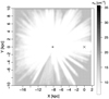 |
Fig. C.1 Predicted uncertainty for our 3D dust map. The Galactic Centre is at (0,0), marked by a cross. The colour shows mean uncertainty along the Z-axis. |
References
- Abolfathi, B., Aguado, D. S., Aguilar, G., et al. 2018, ApJS, 235, 42 [NASA ADS] [CrossRef] [Google Scholar]
- Ballesteros-Paredes, J., Román-Zúñiga, C., Salomé, Q., Zamora-Avilés, M., & Jiménez-Donaire, M. J. 2019, MNRAS, 490, 2648 [Google Scholar]
- Bally, J., Langer, W. D., Stark, A. A., & Wilson, R. W. 1987, ApJ, 312, L45 [NASA ADS] [CrossRef] [Google Scholar]
- Bešlic, I., Barnes, A. T., Bigiel, F., et al. 2021, MNRAS, 506, 963 [CrossRef] [Google Scholar]
- Binder, B. A., & Povich, M. S. 2018, ApJ, 864, 136 [CrossRef] [Google Scholar]
- Blanton, M. R., Bershady, M. A., Abolfathi, B., et al. 2017, AJ, 154, 28 [Google Scholar]
- Brand, J., & Blitz, L. 1993, A&A, 275, 67 [NASA ADS] [Google Scholar]
- Brown, A. G. A. 2021, ARA&A, 59, 59 [NASA ADS] [CrossRef] [Google Scholar]
- Cahlon, S., Zucker, C., Goodman, A., Lada, C., & Alves, J. 2024, ApJ, 961, 153 [NASA ADS] [CrossRef] [Google Scholar]
- Cantat-Gaudin, T., Jordi, C., Vallenari, A., et al. 2018, A&A, 618, A93 [NASA ADS] [CrossRef] [EDP Sciences] [Google Scholar]
- Chiappini, C., Matteucci, F., & Romano, D. 2001, ApJ, 554, 1044 [NASA ADS] [CrossRef] [Google Scholar]
- Colombo, D., Hughes, A., Schinnerer, E., et al. 2014, ApJ, 784, 3 [NASA ADS] [CrossRef] [Google Scholar]
- Dame, T. M., & Lada, C. J. 2023, ApJ, 944, 197 [NASA ADS] [CrossRef] [Google Scholar]
- Dame, T. M., Elmegreen, B. G., Cohen, R. S., & Thaddeus, P. 1986, ApJ, 305, 892 [Google Scholar]
- Dame, T. M., Hartmann, D., & Thaddeus, P. 2001, ApJ, 547, 792 [Google Scholar]
- Darling, J., Paine, J., Reid, M. J., et al. 2023, ApJ, 955, 117 [NASA ADS] [CrossRef] [Google Scholar]
- Donovan Meyer, J., Koda, J., Momose, R., et al. 2013, ApJ, 772, 107 [NASA ADS] [CrossRef] [Google Scholar]
- Draine, B. T. 2009, in Cosmic Dust - Near and Far, eds. T. Henning, E. Grün, & J. Steinacker, Astronomical Society of the Pacific Conference Series, 414, 453 [NASA ADS] [Google Scholar]
- Drimmel, R., & Spergel, D. N. 2001, ApJ, 556, 181 [Google Scholar]
- Edenhofer, G., Zucker, C., Frank, P., et al. 2024, A&A, 685, A82 [NASA ADS] [CrossRef] [EDP Sciences] [Google Scholar]
- Eisenstein, D. J., Weinberg, D. H., Agol, E., et al. 2011, AJ, 142, 72 [Google Scholar]
- Elia, D., Molinari, S., Schisano, E., et al. 2017, MNRAS, 471, 100 [NASA ADS] [CrossRef] [Google Scholar]
- Elia, D., Molinari, S., Schisano, E., et al. 2022, ApJ, 941, 162 [NASA ADS] [CrossRef] [Google Scholar]
- Evans I., Neal J., Kim, K.-T., Wu, J., et al. 2020, ApJ, 894, 103 [NASA ADS] [CrossRef] [Google Scholar]
- Faesi, C. M., Lada, C. J., & Forbrich, J. 2018, ApJ, 857, 19 [NASA ADS] [CrossRef] [Google Scholar]
- Freeman, P., Rosolowsky, E., Kruijssen, J. M. D., Bastian, N., & Adamo, A. 2017, MNRAS, 468, 1769 [NASA ADS] [CrossRef] [Google Scholar]
- Gaia Collaboration (Prusti, T., et al.) 2016, A&A, 595, A1 [NASA ADS] [CrossRef] [EDP Sciences] [Google Scholar]
- Gallagher, M. J., Leroy, A. K., Bigiel, F., et al. 2018, ApJ, 858, 90 [NASA ADS] [CrossRef] [Google Scholar]
- GRAVITY Collaboration (Abuter, R., et al.) 2021, A&A, 647, A59 [NASA ADS] [CrossRef] [EDP Sciences] [Google Scholar]
- Green, G. M., Schlafly, E., Zucker, C., Speagle, J. S., & Finkbeiner, D. 2019, ApJ, 887, 93 [NASA ADS] [CrossRef] [Google Scholar]
- Großschedl, J. E., Alves, J., Meingast, S., et al. 2018, A&A, 619, A106 [Google Scholar]
- Henshaw, J. D., Barnes, A. T., Battersby, C., et al. 2023, in Protostars and Planets VII, eds. S. Inutsuka, Y. Aikawa, T. Muto, K. Tomida, & M. Tamura, Astronomical Society of the Pacific Conference Series, 534, 83 [NASA ADS] [Google Scholar]
- Hogg, D. W., Eilers, A.-C., & Rix, H.-W. 2019, AJ, 158, 147 [Google Scholar]
- Jiménez-Donaire, M. J., Bigiel, F., Leroy, A. K., et al. 2019, ApJ, 880, 127 [CrossRef] [Google Scholar]
- Jiménez-Donaire, M. J., Usero, A., Bešlic´, I., et al. 2023, A&A, 676, L11 [NASA ADS] [CrossRef] [EDP Sciences] [Google Scholar]
- Jönsson, H., Holtzman, J. A., Allende Prieto, C., et al. 2020, AJ, 160, 120 [Google Scholar]
- Kainulainen, J., Rezaei, K. S., Spilker, A., & Orkisz, J. 2022, A&A, 659, L6 [NASA ADS] [CrossRef] [EDP Sciences] [Google Scholar]
- Kalberla, P. M. W., & Kerp, J. 2009, ARA&A, 47, 27 [NASA ADS] [CrossRef] [Google Scholar]
- Kauffmann, J., Goldsmith, P. F., Melnick, G., et al. 2017, A&A, 605, L5 [NASA ADS] [CrossRef] [EDP Sciences] [Google Scholar]
- Kawamura, A., Mizuno, Y., Minamidani, T., et al. 2009, ApJS, 184, 1 [NASA ADS] [CrossRef] [Google Scholar]
- Kennicutt, R. C., & Evans, N. J. 2012, ARA&A, 50, 531 [NASA ADS] [CrossRef] [Google Scholar]
- Kollmeier, J. A., Zasowski, G., Rix, H.-W., et al. 2017, arXiv e-prints, [arXiv:1711.03234] [Google Scholar]
- Krumholz, M. R., & McKee, C. F. 2005, ApJ, 630, 250 [Google Scholar]
- Krumholz, M. R., Burkhart, B., Forbes, J. C., & Crocker, R. M. 2018, MNRAS, 477, 2716 [CrossRef] [Google Scholar]
- Kuno, N., Sato, N., Nakanishi, H., et al. 2007, PASJ, 59, 117 [NASA ADS] [Google Scholar]
- Lee, E. J., Miville-Deschênes, M.-A., & Murray, N. W. 2016, ApJ, 833, 229 [NASA ADS] [CrossRef] [Google Scholar]
- Lee, J. C., Sandstrom, K. M., Leroy, A. K., et al. 2023, ApJ, 944, L17 [NASA ADS] [CrossRef] [Google Scholar]
- Leike, R. H., Glatzle, M., & Enßlin, T. A. 2020, A&A, 639, A138 [NASA ADS] [CrossRef] [EDP Sciences] [Google Scholar]
- Leroy, A. K., Schinnerer, E., Hughes, A., et al. 2021, ApJS, 257, 43 [NASA ADS] [CrossRef] [Google Scholar]
- Leung, H. W., Bovy, J., Mackereth, J. T., et al. 2023, MNRAS, 519, 948 [Google Scholar]
- Majewski, S. R., Zasowski, G., & Nidever, D. L. 2011, ApJ, 739, 25 [Google Scholar]
- Majewski, S. R., Schiavon, R. P., Frinchaboy, P. M., et al. 2017, AJ, 154, 94 [NASA ADS] [CrossRef] [Google Scholar]
- Marshall, D. J., Robin, A. C., Reylé, C., Schultheis, M., & Picaud, S. 2006, A&A, 453, 635 [NASA ADS] [CrossRef] [EDP Sciences] [Google Scholar]
- Miville-Deschênes, M.-A., Murray, N., & Lee, E. J. 2017, ApJ, 834, 57 [Google Scholar]
- Morgan, W. W. 1955, Sci. Am., 192, 42 [NASA ADS] [CrossRef] [Google Scholar]
- Oort, J. H., & Muller, C. A. 1952, Mon. Notes Astron. Soc. South Afr., 11, 65 [Google Scholar]
- Ou, X., Eilers, A.-C., Necib, L., & Frebel, A. 2024, MNRAS, 528, 693 [NASA ADS] [CrossRef] [Google Scholar]
- Padoan, P., Federrath, C., Chabrier, G., et al. 2014, in Protostars and Planets VI, eds. H. Beuther, R. S. Klessen, C. P. Dullemond, & T. Henning, 77 [Google Scholar]
- Pety, J., Guzmán, V. V., Orkisz, J. H., et al. 2017, A&A, 599, A98 [NASA ADS] [CrossRef] [EDP Sciences] [Google Scholar]
- Poggio, E., Drimmel, R., Andrae, R., et al. 2020, Nat. Astron., 4, 590 [NASA ADS] [CrossRef] [Google Scholar]
- Querejeta, M., Schinnerer, E., Schruba, A., et al. 2019, A&A, 625, A19 [NASA ADS] [CrossRef] [EDP Sciences] [Google Scholar]
- Reid, M. J., Dame, T. M., Menten, K. M., & Brunthaler, A. 2016, ApJ, 823, 77 [Google Scholar]
- Reid, M. J., Menten, K. M., Brunthaler, A., et al. 2019, ApJ, 885, 131 [Google Scholar]
- Rezaei Kh., S., & Kainulainen, J. 2022, ApJ, 930, L22 [NASA ADS] [CrossRef] [Google Scholar]
- Rezaei Kh., S., Bailer-Jones, C. A. L., Hanson, R. J., & Fouesneau, M. 2017, A&A, 598, A125 [NASA ADS] [CrossRef] [EDP Sciences] [Google Scholar]
- Rezaei Kh., S., Bailer-Jones, C. A. L., Schlafly, E. F., & Fouesneau, M. 2018a, A&A, 616, A44 [NASA ADS] [CrossRef] [EDP Sciences] [Google Scholar]
- Rezaei Kh., S., Bailer-Jones, Coryn A. L., Hogg, David W., & Schultheis, Mathias 2018b, A&A, 618, A168 [NASA ADS] [CrossRef] [EDP Sciences] [Google Scholar]
- Rezaei Kh., S., Bailer-Jones, C. A. L., Soler, J. D., & Zari, E. 2020, A&A, 643, A151 [EDP Sciences] [Google Scholar]
- Rodgers, A. W., Campbell, C. T., & Whiteoak, J. B. 1960, MNRAS, 121, 103 [NASA ADS] [CrossRef] [Google Scholar]
- Roman-Duval, J., Jackson, J. M., Heyer, M., et al. 2009, ApJ, 699, 1153 [CrossRef] [Google Scholar]
- Roman-Duval, J., Jackson, J. M., Heyer, M., Rathborne, J., & Simon, R. 2010, ApJ, 723, 492 [NASA ADS] [CrossRef] [Google Scholar]
- Romero-Gómez, M., Antoja, T., Figueras, F., et al. 2019, in Highlights on Spanish Astrophysics X, eds. B. Montesinos, A. Asensio Ramos, F. Buitrago, et al., 386 [Google Scholar]
- Russeil, D. 2003, A&A, 397, 133 [CrossRef] [EDP Sciences] [Google Scholar]
- Schinnerer, E., Meidt, S. E., Pety, J., et al. 2013, ApJ, 779, 42 [Google Scholar]
- Skrutskie, M. F., Cutri, R. M., Stiening, R., et al. 2006, AJ, 131, 1163 [NASA ADS] [CrossRef] [Google Scholar]
- Sun, J., Leroy, A. K., Schinnerer, E., et al. 2020, ApJ, 901, L8 [NASA ADS] [CrossRef] [Google Scholar]
- Sun, J., Leroy, A. K., Rosolowsky, E., et al. 2022, AJ, 164, 43 [NASA ADS] [CrossRef] [Google Scholar]
- Tafalla, M., Usero, A., & Hacar, A. 2021, A&A, 646, A97 [NASA ADS] [CrossRef] [EDP Sciences] [Google Scholar]
- Tafalla, M., Usero, A., & Hacar, A. 2023, A&A, 679, A112 [NASA ADS] [CrossRef] [EDP Sciences] [Google Scholar]
- van de Hulst, H. C., Muller, C. A., & Oort, J. H. 1954, BAN, 12, 117 [NASA ADS] [Google Scholar]
- Vergely, J. L., Lallement, R., & Cox, N. L. J. 2022, A&A, 664, A174 [NASA ADS] [CrossRef] [EDP Sciences] [Google Scholar]
- Westerhout, G. 1958, Bull. Astron. Inst. Netherlands, 14, 215 [NASA ADS] [Google Scholar]
- Wright, E. L., Eisenhardt, P. R. M., Mainzer, A. K., et al. 2010, AJ, 140, 1868 [Google Scholar]
- Zasowski, G., Johnson, J. A., Frinchaboy, P. M., et al. 2013, AJ, 146, 81 [NASA ADS] [CrossRef] [Google Scholar]
- Zucker, C., Goodman, A., Alves, J., et al. 2021, ApJ, 919, 35 [NASA ADS] [CrossRef] [Google Scholar]
All Tables
All Figures
|
Fig. 1 Final sample used as our input data. The top panel shows the X-Y plane, which is perpendicular to the Galactic plane, and the bottom panel presents the X − Z plane where our cut on the 1 kpc Galactic height is visible. The colour shows estimated extinctions for individual stars. The Sun is at (−8.2,0,0) and the Galactic centre is marked with an X, assuming the Sun is at the distance of 8.2 kpc from the Galactic centre. The gaps between different LOSs indicate that the sky is not observed uniformly by APOGEE. |
| In the text | |
|
Fig. 2 Frontal view of our 3D map of dust in Galactic plane for different Galactic heights. The bottom right panel shows the combined map from -750 pc to 750 pc in the Galactic height. The colour shows the mean of our predicted density (cm−3) for each pixel (100×100 in X − Y plane) in all panels, except for the bottom right where the colour represents the maximum density within the 1.5 kpc height. The Sun is at (−8.2,0,0) and the Galactic centre is marked with an ×, assuming the Sun is 8.2 kpc from the Galactic centre. White regions are areas devoid of input data. |
| In the text | |
|
Fig. 3 Frontal view of 3D map for all Galactic heights. Left panel: same as bottom right panel of Fig. 2, in addition to having shaded areas illustrating regions of high uncertainty (fractional uncertainties larger than 50%). Right panel: clouds selected from 3D map whose density values lie three standard deviations above the mean of the Gaussian process. This corresponds to densities above 80 cm−3. |
| In the text | |
|
Fig. 4 Example of how clouds in Table A.1 are assigned to known structures and spiral arms. The black line with the blue shaded uncertainties are our density predictions as a function of distance for a given LOS, and the purple vertical lines are all probable distance estimates from the BESSEL survey (Reid et al. 2016) for the same LOS with velocities observed in Dame et al. (1986) (e.g. Aquila rift, Sagittarius Near, and Perseus here). The dashed red line indicates our threshold for selecting statistically significant clouds. If there is a match, such as the near Sagittarius Arm in the middle, we assign the cloud to that particular structure. The LOS’ galactic longitude and latitude are shown in the top right corner. |
| In the text | |
|
Fig. 5 Comparison of locations of high-density dust in 3D dust maps of Galactic plane. Grids are drawn for easier comparisons between maps. The lower right panel shows our 3D map where dashed lines represent identified large cavities. Similar cavities are seen in the upper right panel representing the work of Vergely et al. (2022). While matching cavities seem to be present at similar locations in the other two panels, (Green et al. 2019; Marshall et al. 2006), due to substantial artefacts a direct comparison appears difficult. Apart from our map, only the work of Marshall et al. (2006) expands beyond the Galactic centre; despite the elongated artefacts, multiple over-densities in the first quadrant and towards the Galactic centre are evident on both maps. The range and the width of the maps along the Z direction vary; Vergely et al. (2022) covered from Z=−400 pc to Z=400 pc and provides extinction densities ranging between 0 and 5 × 10⁻³ mag/pc, while Green et al. (2019) covered Z=−300 pc to Z=300 pc and provides differential extinction ranging from 0 to 0.5 mag/kpc. Marshall et al. (2006) covered |b| ≤ 0.25 and represents average extinction density of 0–0.4 kpc−1. |
| In the text | |
|
Fig. 6 Grey scale showing clouds extracted from our 3D dust map (same as Fig. 3, right). The colour-coding follows the same as Fig. 1 in Reid et al. (2019). Each colour represents masers belonging to a spiral arm as follows: 3-kpc arm: yellow – Norma–Outer arm: red – Scutum–Centaurus–OSC arm: blue – Sagittarius–Carina arm: purple – Local arm: cyan – Perseus arm: black. The Green points are equivalent to the white points in Reid et al. (2019), illustrating spurs or sources with unclear arm associations. |
| In the text | |
|
Fig. 7 Comparison between our clouds and molecular clouds observed in CO. Left panel: 3D distribution of molecular clouds observed in CO from Miville-Deschênes et al. (2017), with our extracted clouds over-plotted as contours. Right panel: longitude-velocity plot of molecular clouds from the left, situated underneath our cloud contours. The colour shows the surface density of clouds derived in Miville-Deschênes et al. (2017). |
| In the text | |
|
Fig. 8 Mass as function of galactocentric radius for clouds from our 3D map (top) and CO from Miville-Deschênes et al. (2017) (bottom) for galactocentric rings of 1 kpc thickness. In this plot, we exclude CO clouds from Miville-Deschênes et al. (2017) belonging to regions not covered by our map (e.g. parts of the fourth quadrant). The shaded area shows regions where our results are likely underestimated due to the lack of input data. We did not limit the azimuth range for each radial bin; however, due to the limitations in the map, for regions beyond a galactocentric radius of 2 kpc, our radial average only covers half of a circle (negative X in previous figures). |
| In the text | |
|
Fig. 9 Comparison of volume density and column density. Left panel: volume densities of clouds from our 3D map (same as Fig. 3, right). Right panel: column densities of left side clouds integrated over the Z access. |
| In the text | |
|
Fig. B.1 An aitoff view of the input data representing the pointing pattern of the APOGEE. Most of the data is concentrated in the Galactic Plane, and the Northern Hemisphere with few observations in the Southern Hemisphere as well. colour represents the mean extinction per pixel. |
| In the text | |
|
Fig. C.1 Predicted uncertainty for our 3D dust map. The Galactic Centre is at (0,0), marked by a cross. The colour shows mean uncertainty along the Z-axis. |
| In the text | |
Current usage metrics show cumulative count of Article Views (full-text article views including HTML views, PDF and ePub downloads, according to the available data) and Abstracts Views on Vision4Press platform.
Data correspond to usage on the plateform after 2015. The current usage metrics is available 48-96 hours after online publication and is updated daily on week days.
Initial download of the metrics may take a while.