© The Authors 2024

1. Introduction

The magnetic field is one of the key ingredients required in our efforts to understand the dynamical evolution of molecular clouds and prestellar cores (Mouschovias & Ciolek 1999). Observationally, our knowledge of the magnetic field in molecular clouds mostly stems from polarized thermal dust emission (e.g., Ward-Thompson et al. 2017) and dust-induced starlight polarization (e.g., Panopoulou et al. 2016). Both of these techniques probe the orientation of the plane-of-sky (POS) component of the magnetic field, while its strength can be measured under certain assumptions regarding the equipartition between the kinetic and magnetic energy (Davis 1951; Chandrasekhar & Fermi 1953; see also Skalidis & Tassis 2021 and references therein).

On the other hand, the line-of-sight (LOS) component of the magnetic field can be probed by Zeeman circular polarization measurements of molecular spectral lines (e.g., Troland & Crutcher 2008; Falgarone et al. 2008). The Zeeman effect remains the only available method that can directly yield the strength of the magnetic field (as well as its direction) and it is therefore extremely valuable. However, due to the very high signal-to-noise ratio required, robust measurements of the Zeeman effect can be extremely challenging, often requiring as much as ∼10 hours of integration time per pointing (Crutcher et al. 2009).

On the subject of radio observations of molecular spectra, one of the most under-explored techniques for probing the direction of magnetic fields is linear polarization of spectral lines. Linear polarization of molecular spectral lines in interstellar clouds can arise when the magnetic sublevels are unequally populated due to an anisotropic radiation field. This effect is commonly known as the Goldreich-Kylafis (“GK”) effect within the interstellar medium community (Goldreich & Kylafis 1981), but it is important to note that it is a very well-known effect in physics (see, e.g., Lamb & Ter Haar 1971; Happer 1972) and solar physics (see, e.g., House 1970; Landi Degl’Innocenti 1978; Stenflo et al. 1980). For this effect to arise, the optical depth of the line needs to be moderate and anisotropic and the radiative rates need to be comparable to the collisional ones for excitation and de-excitation. Therefore, linear polarization in spectral lines caused by anisotropic radiation pumping arises only under non-local thermodynamic equilibrium (non-LTE) conditions. Linear polarization of spectral lines is also shown to arise in masers (Goldreich et al. 1973; Deguchi & Watson 1990; Lankhaar & Vlemmings 2019), in circumstellar envelopes through directional continuum emission in evolved stars (Morris et al. 1985), and in star-forming regions via directional collisions (Lankhaar & Vlemmings 2020b). Finally, linearly polarized radiation can be transformed to circular polarized through the so-called anisotropic resonant scattering effect (Houde et al. 2022 and references therein).

In the context of solar physics, linear polarization of spectral lines arising due to the anisotropy of the radiation field within the solar photosphere and chromosphere has been observed for decades (e.g., Stenflo et al. 1980; Stenflo & Keller 1997). In the presence of a magnetic field, this linear polarization caused by anisotropic radiation pumping is modified by the Hanle effect (Hanle 1924), which typically produces depolarization and rotation of the plane of polarization, depending on the angle of scattering and the magnetic field (see Fig. 1 of Trujillo Bueno 2001 for a comprehensive description of all the different cases). Many spectropolarimetric observations have been used to infer information on the magnetic field in the solar atmosphere (see the review by Trujillo Bueno & del Pino Alemán 2022; for a detailed presentation of the quantum theory of polarization in spectral lines, see Landi Degl’Innocenti & Landolfi 2004).

In the prestellar phase of molecular clouds, only a handful of observational surveys of linear polarization of molecular spectra have been reported to date Lai et al. (2003), Girart et al. (2004), Cortes et al. (2005), Forbrich et al. (2008), Cortés et al. (2021), Barnes et al. (2023). However, on the theoretical front, the theoretical formalisms for modeling polarization in spectral lines were developed more than five decades ago (Lamb & Ter Haar 1971; Landi Degl’Innocenti 1978; Goldreich & Kylafis 1981, 1982; Kylafis 1983; Landi Degl’Innocenti 1983; Deguchi & Watson 1984; Landi Degl’Innocenti & Landolfi 2004; Cortes et al. 2005; Yang & Lai 2010; Huang et al. 2020). Lankhaar & Vlemmings (2020a) recently developed the PORTAL (POlarized Radiative Transfer Adapted to Line) radiative-transfer code, which builds upon the non-polarized results from the LIME (Line Modeling Engine; Brinch & Hogerheijde 2010) radiative-transfer code to yield the polarization fraction. However, in PORTAL, only the anisotropy of the total radiation is considered, instead of the two polarization modes of the radiation being considered individually. Even though Lankhaar & Vlemmings (2020a) demonstrated the validity of their approximation in specialized cases where they found deviations from the results by (Goldreich & Kylafis 1981) only for high optical depths, it remains ambiguous how well their approximation performs in the general case. PORTA (Štěpán & Trujillo Bueno 2013), which is primarily used within the solar physics community, is another radiative-transfer code capable of modeling both the linear polarization of spectral lines (in different regimes with respect to magnetic-field strength and morphology) and the Zeeman effect.

Here, we modify the PYRATE (Python Radiative Transfer Emission) code (Tritsis et al. 2018) to include linear polarization of molecular lines following the theoretical formalism by Deguchi & Watson (1984). Under this multilevel formalism, the different modes of polarized radiation are considered individually. In contrast to other radiative-transfer codes (e.g., RADEX; van der Tak et al. 2007), the optical depth in PYRATE is computed more accurately by taking into account variations in all relevant physical quantities, that is, the H₂ number density, the molecular number density, the temperature, and the velocity structure of the physical system under consideration¹. We note, however, that a more general non-LTE theoretical formalism than that by Deguchi & Watson (1984) for the generation and transfer of polarized radiation in the presence of arbitrary magnetic fields is the one described in Landi Degl’Innocenti & Landolfi (2004).

This study is organized as follows. In Sect. 2, we outline the theoretical background and basic equations. In Sect. 3, we benchmark our code by performing various tests for limiting cases and by comparing our numerical calculations against analytical results. In Sect. 4, we present polarized line radiative-transfer calculations from a nonideal magnetohydrodynamic (MHD) simulation of a collapsing prestellar core, where the number density of CO is computed on the fly using a non-equilibrium chemical model. Finally, we summarize our results and conclude in Sect. 5. In order to maintain focus to the physical aspects of the effect, we defer the discussion of numerical details to Appendix B.

2. Basic equations and implementation

Figure 1 schematically depicts all the processes that need to be considered for a linear molecule with three rotational levels, when the magnetic sublevels are considered individually. Here, we have separated between spontaneous emission, absorption and stimulated emission, and collisional excitation and de-excitation processes. Compared to the case where the population densities are (2J+1) times degenerate, the level of complication increases substantially. Specifically, we need to consider all the spontaneous and stimulated emission and absorption processes allowed by the selection rules (ΔJ = 1, |Δm| = 0, 1) separately. Additionally, for collisional processes we need to consider all the possible transitions between every sublevel. Most significantly however, for each pair of rotational levels J and J − 1 (henceforth denoted as J′), two sets of escape probabilities need to be computed (one for each polarization mode), instead of one. To make matters even more complicated, the escape probability associated with the specific intensity polarized parallel to the magnetic field (I_J, J′^∥) depends upon the angle between the direction of propagation of radiation with the magnetic field (henceforth denoted as γ).

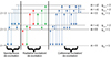Fig. 1. Schematic representation of all the processes considered for a molecular species with three rotational energy levels, when the magnetic sublevels are considered independently. Absorption and stimulated emission associated with Δm = 0 are marked with red, while the corresponding transitions associated with |Δm| = 1 are marked in green.

In the following, the net radiative rates associated with transitions with Δm = 0 and |Δm| = 1 are denoted, respectively, with ℛ_J, J′ and 𝒰_J, J′. For the rest of the quantities, we follow the notation by Deguchi & Watson (1984). The quantities ℛ_J, J′ and 𝒰_J, J′ are given by

$$\begin{array}{cc}\hfill {\mathcal{R}}_{J,J\prime }& =3B_{J,m\to J\prime ,m\prime }{\displaystyle \int \frac{\mathrm{d}\mathrm{\Omega }}{4\pi }}{sin}^2\gamma {\displaystyle \int \mathrm{d}\nu }\varphi (\nu -{\nu }_{J,J\prime })I_{J,J^{\prime }}^{\Vert }(\widehat{\mathbf{\Omega }}),\hfill \end{array}$$(1a)

$$\begin{array}{cc}\hfill {\mathcal{U}}_{J,J\prime }& =\frac{3B_{J,m\to J\prime ,m\prime }}{2}{\displaystyle \int \frac{\mathrm{d}\mathrm{\Omega }}{4\pi }\int \mathrm{d}\nu }\varphi (\nu -{\nu }_{J,J\prime })\hfill \\ \hfill & \{I_{J,J^{\prime }}^{\perp }(\widehat{\mathbf{\Omega }})+{cos}^2\gamma I_{J,J^{\prime }}^{\Vert }(\widehat{\mathbf{\Omega }})\},\hfill \end{array}$$(1b)

where ν and ν_J, J′ are, respectively, the frequency, and the rest frequency of the line. Furthermore, $\widehat{\mathbf{\Omega }}$ is the unit vector of the direction of propagation of the radiation, B_{J, m → J′,m′} is the Einstein B coefficient for stimulated emission, ϕ(ν − ν_J, J′) is the normalized profile function, and I_J, J′^⊥ denotes the specific intensity of radiation polarized perpendicular to the magnetic field.

Under the large-velocity-gradient (LVG) approximation (Sobolev 1960; Castor 1970; Lucy 1971), we have that

$$\begin{array}{c}\hfill {\displaystyle \int \mathrm{d}\nu \varphi }(\nu -{\nu }_{J,J\prime })I_{J,J^{\prime }}^q=S_{J,J\prime }^q(1-{\beta }_{J,J^{\prime }}^q)+\frac{B}{2}{\beta }_{J,J^{\prime }}^q,\end{array}$$(2)

where q = ∥ or ⊥, β is the probability that a photon escapes the cloud, and S_J, J′^q is the source function. The second term on the right-hand side of Eq. (2) represents the contribution due to external photons penetrating the cloud. Here, we assume that the only external radiation is due to the cosmic microwave background (CMB; henceforth denoted as B_CMB). Following Cortes et al. (2005), a compact external continuum source can also be added to the code by setting $B=B_{\mathrm{CMB}}+\mathcal{S}(\widehat{\mathbf{\Omega }})$ where

$$\begin{array}{c}\hfill \mathcal{S}(\widehat{\mathbf{\Omega }})=(1-e^{-{\tau }_c})B_{\nu }(T_{\mathrm{source}}).\end{array}$$(3)

In Eq. (3), B_ν(T_source) and T_source are, respectively, Planck’s function and the temperature of the continuum source, and τ_c is the optical depth for continuum emission from the source. For further details on adding an external continuum source, we refer the reader to Cortes et al. (2005). The escape probability is related to the optical depth of the line as β_J, J′^q = (1 + e^{−τ_J′,Jq})/τ_J′,J^q (Mihalas 1978; de Jong et al. 1980²). Although, in strict terms, the latter equation holds true only under the LVG approximation, one can still physically expect that an escape probability can be defined even when the velocity gradients in the physical system of interest are not large enough for the LVG to be valid. In the interest of consistency throughout all of our numerical results presented herewith, we make use of the latter equation both for physical systems that satisfy the LVG approximation (see Sect. 3) and for non-LVG systems (see Sect. 4). In turn, the optical depth of the radiation polarized parallel and perpendicular to the magnetic field can be computed by integrating the absorption coefficient κ_J′,J^q, which is given by

$$\begin{array}{cc}\hfill {\kappa }_{J\prime ,J}^{\perp }& =\frac{1}{2}\varphi (\nu -{\nu }_{J,J\prime }){\displaystyle \sum _{\mathrm{\Delta }m=1}}{\kappa }_{J\prime ,m\prime \to J,m}\hfill \end{array}$$(4a)

$$\begin{array}{cc}\hfill {\kappa }_{J\prime ,J}^{\Vert }& =\varphi (\nu -{\nu }_{J,J\prime })({sin}^2\gamma {\displaystyle \sum _{\mathrm{\Delta }m=0}}{\kappa }_{J\prime ,m\prime \to J,m}\hfill \\ \hfill & +\frac{1}{2}{cos}^2\gamma {\displaystyle \sum _{\mathrm{\Delta }m=1}}{\kappa }_{J\prime ,m\prime \to J,m}).\hfill \end{array}$$(4b)

In Eqs. (4a) and (4b), κ_{J′,m′→J, m} is computed as

$$\begin{array}{cc}\hfill {\kappa }_{J\prime ,m\prime \to J,m}& =\frac{3}{8\pi }(\frac{c}{{\nu }_{J,J\prime }}{)}^2{A}_{J,m\to J\prime ,m\prime }max(g_{J,m},g_{J\prime ,m\prime })\hfill \\ \hfill & (n_{J\prime ,m\prime }-n_{J,m}),\hfill \end{array}$$(5)

where c is the speed of light, g_J, m is the statistical weight, A_{J, m → J′, m′} is the Einstein A coefficient, and n_J′, m′ and n_J, m are the level populations of the lower and upper energy sublevels, respectively. The level populations can be computed by solving the detailed balance equations (see Appendix A). While solving the detailed balance equations and throughout the code, we impose that n_J, m = n_J, −m (for m ≠ 0). The term max(g_J, m, g_J′, m′) that appears in Eq. (5) ensures, however, that every process that needs to be considered twice (e.g., (2, |2|) → (1, |1|) or in other words, from level (2, 2) to (1, 1) and from level (2, −2) to level (1, −1)), is correctly being done so. Finally, the source functions S_J, J′^q that appears in Eq. (2) are given by

$$\begin{array}{cc}\hfill S_{J,J\prime }^{\perp }& =\frac{{\displaystyle {\sum }_{\mathrm{\Delta }m=1}}{\kappa }_{J\prime ,m\prime \to J,m}{S}_{J,m\to J\prime ,m\prime }}{{\displaystyle {\sum }_{\mathrm{\Delta }m=1}}{\kappa }_{J\prime ,m\prime \to J,m}},\hfill \end{array}$$(6a)

$$\begin{array}{cc}\hfill S_{J,J\prime }^{\Vert }& =({sin}^2\gamma {\displaystyle \sum _{\mathrm{\Delta }m=0}}{\kappa }_{J\prime ,m\prime \to J,m}{S}_{J,m\to J\prime ,m\prime }\hfill \\ \hfill & +\frac{1}{2}{cos}^2\gamma {\displaystyle \sum _{\mathrm{\Delta }m=1}}{\kappa }_{J\prime ,m\prime \to J,m}{S}_{J,m\to J\prime ,m\prime })\hfill \\ \hfill & ({sin}^2\gamma {\displaystyle \sum _{\mathrm{\Delta }m=0}}{\kappa }_{J\prime ,m\prime \to J,m}+\frac{1}{2}{cos}^2\gamma {\displaystyle \sum _{\mathrm{\Delta }m=1}}{\kappa }_{J\prime ,m\prime \to J,m}{)}^{-1},\hfill \end{array}$$(6b)

where

$$\begin{array}{c}\hfill S_{J,m\to J\prime ,m\prime }=\frac{h{\nu }_{J,J\prime }^3}{c^2}\frac{n_{J,m}}{n_{J\prime ,m\prime }-n_{J,m}}.\end{array}$$(7)

In Eq. (7), h is Planck’s constant.

The optical depth, τ_J′,J^q, for each polarization direction for a grid point (i′,j′,k′), is calculated by adding the absorption coefficient of the grid points for which their velocity difference with grid point (i′,j′,k′) is less than the thermal linewidth (see also the discussion in Appendix C). For instance, the optical depth in the x⁺ and x⁻ directions is

$$\begin{array}{cc}\hfill {\tau }_{J^{\prime },J}^{q,x^{+}}& =(\frac{{\kappa }_{J\prime ,J,i\prime j\prime k\prime }^q}{2}+{\displaystyle \sum _{i=i^{\prime }+1}^{N_x}}{\kappa }_{J\prime ,J,ijk}^q[\mid v_{i^{\prime }{j}^{\prime }{k}^{\prime }}-v_{i{j}^{\prime }{k}^{\prime }}\mid <\mathrm{\Delta }{v}_{i{j}^{\prime }{k}^{\prime }}^{\mathit{th}}])\mathrm{\Delta }x\hfill \end{array}$$(8a)

$$\begin{array}{cc}\hfill {\tau }_{J^{\prime },J}^{q,x^{-}}& =(\frac{{\kappa }_{J\prime ,J,i\prime j\prime k\prime }^q}{2}+{\displaystyle \sum _{i=i^{\prime }-1}^0}{\kappa }_{J\prime ,J,ijk}^q[\mid v_{i^{\prime }{j}^{\prime }{k}^{\prime }}-v_{i{j}^{\prime }{k}^{\prime }}\mid <\mathrm{\Delta }{v}_{i{j}^{\prime }{k}^{\prime }}^{\mathit{th}}])\mathrm{\Delta }x,\hfill \end{array}$$(8b)

where N_x is the size of our grid in the x direction, Δx is the size of the cell in the same direction, v is the velocity, and Δv^th is the thermal linewidth. An identical process is adopted for the y and z directions as well as for all the secondary diagonals (“$d_{x\mathit{y},xz,\mathit{y}z}^{\pm }$”) and anti-diagonals (“${\overline{d}}_{x\mathit{y},xz,\mathit{y}z}^{\pm }$”) in each grid point (i.e., the directions defined by the unit vectors (1/$\sqrt{2}$, 1/$\sqrt{2}$, 0), (−1/$\sqrt{2}$, 1/$\sqrt{2}$, 0), (1/$\sqrt{2}$, −1/$\sqrt{2}$, 0), (−1/$\sqrt{2}$, −1/$\sqrt{2}$, 0) and so on and so forth). Consequently, for each pair of rotational levels, J, J′, we compute 18 optical depths for each polarization direction. Then, we numerically solve the integrals in Eqs. (1a and 1b) by computing a value for the optical depth for every direction, $\widehat{\mathbf{\Omega }}$, as

$$\begin{array}{c}\hfill \frac{1}{\tau (\widehat{\mathbf{\Omega }})}=\frac{{\displaystyle \sum _{n=1}^{18}}\frac{1}{{\tau }_n}(\widehat{\mathbf{\Omega }}·{\widehat{\mathit{w}}}_{\mathit{n}}[{cos}^{-1}(\widehat{\mathbf{\Omega }}·{\widehat{\mathit{w}}}_{\mathit{n}})<90]{)}^2}{{\displaystyle \sum _{n=1}^{18}}(\widehat{\mathbf{\Omega }}·{\widehat{\mathit{w}}}_{\mathit{n}}[{cos}^{-1}(\widehat{\mathbf{\Omega }}·{\widehat{\mathit{w}}}_{\mathit{n}})<90]{)}^2},\end{array}$$(9)

where ${\widehat{\mathit{w}}}_{\mathit{n}}$ are the unit vectors along the principle axes, secondary diagonals and anti-diagonals (both directions) and τ_n are the values of the optical depth along these directions. As an example, in Fig. 2 we show the interpolated values of the optical depth in every direction $\widehat{\mathbf{\Omega }}$ for arbitrary choices τ_n along each of the 18 directions described above.

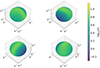Fig. 2. Interpolated values of the optical depth inside a single cell, based on Eq. (9), along each direction $\widehat{\mathbf{\Omega }}$. In this example, the values of the optical depth in the directions x+, x−, y+, y−, $z^{+},z^{-},d_{x\mathit{y}}^{+},d_{x\mathit{y}}^{-},{\overline{d^{+}}}_{x\mathit{y}},{\overline{d^{-}}}_{x\mathit{y}},d_{\mathit{xz}}^{+},d_{\mathit{xz}}^{-},{\overline{d^{+}}}_{\mathit{xz}},{\overline{d^{-}}}_{\mathit{xz}},d_{\mathit{y}z}^{+},d_{\mathit{y}z}^{-},{\overline{d^{+}}}_{\mathit{y}z}$ and ${\overline{d^{-}}}_{\mathit{y}z}$ are equal to 14, 7, 6, 0.5, 7, 5, 2, 1.5, 5, 13, 9, 6, 9, 8, 4, 3, 10 and 3, respectively.

For the Einstein A coefficient that first appeared in Eq. (5), Deguchi & Watson (1984) reference Townes & Schawlow (1955) and adopt

$$\begin{array}{c}\hfill A_{J,m\to J\prime ,m\prime }=\begin{array}{c}\frac{{(J+1)}^2-m^2}{(2J+1)(J+1)}{A}_{J\to J\prime },\text{for}\mathrm{\Delta }m=0\hfill \\ \frac{(J+|m|+1)(J+|m|)}{2(2J+1)(J+1)}{A}_{J\to J\prime },\text{for}|\mathrm{\Delta }m|=1,\hfill \end{array}\end{array}$$(10)

where the value of A_{J → J′} can be found in databases for molecular spectroscopy such as the LAMBDA database (Schöier et al. 2005). However, the expression given in Eq. (10) is not correct and should not be used as it leads to non-negligible linear polarization (on the order of a few %) even under LTE conditions. Instead, the Einstein A coefficient should be computed as (Stenflo 1994)

$$\begin{array}{c}\hfill A_{J,m\to J\prime ,m\prime }=(2J+1){\left(\begin{array}{ccc}J& 1& J\prime \\ -m& m-m\prime & m\prime \end{array}\right)}^2{A}_{J\to J\prime },\end{array}$$(11)

where the term in the brackets is the Wigner 3j symbol³. For the transition J = 1 → 0, Eq. (11) gives that A_{1, 0 → 0, 0} = A_{1, ± 1 → 0, 0} = A_1 → 0, meaning that spontaneous transitions between all three sublevels are equally likely⁴. On the other hand, Eq. (10) gives $A_{1,0\to 0,0}=\frac{2}{3}{A}_{1\to 0}$ and $A_{1,\pm 1\to 0,0}=\frac{1}{2}{A}_{1\to 0}$. Clearly, adopting Eq. (10) instead of Eq. (11) will lead to the magnetic sublevels of J = 1 having unequal populations, even without stimulated processes taken into account.

For the collisional coefficients, we follow Deguchi & Watson (1984) and adopt

$$\begin{array}{c}\hfill C_{J,m\to J\prime ,m\prime }=\frac{C_{J\to J\prime }}{(2J\prime +1)}.\end{array}$$(12)

Eq. (12) implies that the collisional processes for each magnetic sublevel are treated equally. Finally, given that we have no knowledge regarding the collisional coefficients between magnetic sublevels (hereafter denoted as $C{\prime }_{m\to m\prime }$), we assume that $C{\prime }_{m\to m\prime }=C_{J,m\to J\prime ,m\prime }$ for all of our tests, unless otherwise stated. However, in our numerical implementation, the collisional coefficients between magnetic sublevels can be scaled as $C{\prime }_{m\to m\prime }=f_{\mathit{GK}}\times C_{J,m\to J\prime ,m\prime }$, where f_GK is a user-defined variable.

Finally, once the level populations are calculated, we compute the specific intensity for every frequency and position (l, b) on the front face of the simulation (i.e., the “plane of the sky”) by integrating the radiative-transfer equation for all points “k” along the line of sight

$$\begin{array}{c}\hfill I_{k+1}^q=\frac{(e^{-{\tau }_{k+1}^C}-{\zeta }^q)I_k^q+{\zeta }^q{S}_k^q+{\xi }^q{S}_{k+1}^q+\mathcal{S}}{1+{\xi }^q}\end{array}$$(13)

where τ^C is the optical depth for continuum emission and 𝒮 is a function of the source function for dust-continuum emission, and the optical depth and absorption coefficient for continuum (see Eq. (4) from Tritsis et al. 2018). For more details on the dust model used, we refer the reader to Tritsis et al. (2018). The quantities ξ and ζ are defined as

$$\begin{array}{c}\hfill \xi =\frac{{\tau }_{k+1}^q}{1+e^{-{\tau }_{k+1}^q}}\end{array}$$(14)

$$\begin{array}{c}\hfill \zeta =\xi (e^{-{\tau }_{k+1}^q-{\tau }_{k+1}^C})\end{array}$$(15)

where the optical depth for line emission τ^q is calculated by integrating the absorption coefficient between points “k” and “k + 1” and for the normalized profile function we use

$$\begin{array}{c}\hfill \varphi =\frac{1}{\mathrm{\Delta }{\nu }_{i,j,k}\sqrt{\pi }}{e}^{-(\frac{\nu -{\nu }_{J,J\prime }(1+\frac{{\widehat{\mathit{w}}}_{\mathrm{LOS}}·{\mathit{v}}_{\mathit{i}\mathbf{,}\mathit{j}\mathbf{,}\mathit{k}}}{c})}{\mathrm{\Delta }{\nu }_{i,j,k}}{)}^2}\end{array}$$(16)

where ${\widehat{\mathit{w}}}_{\mathrm{LOS}}$ is the unit vector that defines the LOS direction, ${\mathit{v}}_{\mathit{i}\mathbf{,}\mathit{j}\mathbf{,}\mathit{k}}$ is the velocity of grid point (i, j, k) and Δν_i, j, k is the thermal width in frequency units, defined as

$$\begin{array}{c}\hfill \mathrm{\Delta }{\nu }_{i,j,k}=\sqrt{\frac{2k_B{T}_{i,j,k}}{m_{\mathrm{mol}}{c}^2}}{\nu }_{J,J\prime }\end{array}$$(17)

where, in turn, k_B is the Boltzmann constant and m_mol is the mass of the emitting species.

The formalism presented above is valid under the so-called strong magnetic field limit (Goldreich & Kylafis 1981, 1982) where the magnetic precession rate exceeds the collisional and radiative rates. For a linear molecule such as CO with a g value (not to be confused with the statistical weight g_J, m) of ∼0.27 (Meerts et al. 1977) the magnetic precession rate is, at least, 3–4 orders of magnitude larger than the collisional and radiative rates throughout the isothermal phase of molecular clouds (e.g., n_H2 = 300 − 10¹⁰ cm⁻³). Therefore, this condition is always very well satisfied. For a 3D non-LTE radiative transfer code that can model linear polarization when this condition is not satisfied we refer the reader to PORTA (Štěpán & Trujillo Bueno 2013).

In the present formalism we have also implicitly assumed that Stokes U is zero (see Eqs. 44–46 in Goldreich & Kylafis 1982). This is a rigorous assumption for a uniform magnetic field or for a system satisfying the LVG approximation given there is one-to-one correlation between frequency or velocity and physical space. However, as we show in Appendix D, even for a non-LVG system with a varying magnetic field along the LOS, the errors introduced are marginal. As was already noted in Sect. 1, a more powerful theoretical formalism for modeling the transfer of polarized radiation in the presence of arbitrary magnetic fields is that developed by Landi Degl’Innocenti & Landolfi (2004).

3. Benchmarking

For our initial radiative-transfer tests, we use as input a 2D cylindrical, isothermal, nonideal MHD chemo-dynamical simulation of a collapsing prestellar core. The initial and physical conditions of this MHD simulation were presented in Tritsis et al. (2023) (see also Tritsis et al. 2022 for a detailed description of the methodology followed for performing such MHD chemo-dynamical simulations). We use a model with a temperature of T = 10 K, visual extinction of A_v = 10, and a standard cosmic-ray ionization rate (ζ = 1.3 × 10⁻¹⁷ s⁻¹; Caselli et al. 1998). The initial density was uniform and set equal to n_H2 = 300 cm⁻³, which, given the dimensions of the cloud (r_max = z_max = 0.75 pc), translates to a total mass of ∼45 M_⊙. The initial magnetic field was constant everywhere and aligned to the axis of symmetry, and its strength was set equal to 15 μG. Consequently, the initial mass-to-flux ratio (normalized to the critical value; Mouschovias & Spitzer 1976) was 1/2 (see Table 1 of Tritsis et al. 2023). Finally, the cloud had initially zero kinetic energy.

We post-process this chemo-dynamical simulation when the central density is n_H2 = 5 × 10⁴ cm⁻³. At this evolutionary stage, the strength of the magnetic field in the central high-density regions of the cloud is ∼36 μG whereas at the outskirts it remains at 15 μG. Such values are consistent with the range of values found in the diffuse and higher-density regions in Taurus (e.g., Chapman et al. 2011). In Fig. 3 we show the H₂ and CO number densities in the left and right panels, respectively. The orange streamlines overlaid on top of the H₂ number density show the magnetic field lines and the color-coded blue vectors show the velocity field⁵. The velocity field observed in the left panel of Fig. 3 is a result of the cloud rebounding after the initial thermal relaxation phase (see Tritsis et al. 2022; Kunz & Mouschovias 2010 for more details). Given the hourglass morphology in our MHD simulation, the magnetic-field direction can exhibit variations of ∼10° with respect to the LOS. In the following, we use r and z when we refer to the actual computational region of the chemo-dynamical simulation (i.e., the set of coordinates that can be translated to 3D space) and R and Z to denote coordinates after ray-tracing through our computational region (i.e., the POS).

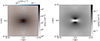Fig. 3. H2 and CO number densities (left and right panels, respectively) from a nonideal MHD chemo-dynamical simulation. Orange streamlines in the left panel depict the magnetic field lines and the color-coded vectors show the velocity in the cloud. This simulation is used as the underlying physical model in Sect. 3.1, Sect. 3.2, and Sect. 4.

The nonideal MHD chemo-dynamical simulation described above was used as an input to PYRATE for the radiative-transfer simulations presented in Sect. 3.1, Sect. 3.2, and Sect. 4. In the same sections as well as in Sect. 3.4, we adopt the Einstein and collisional coefficients, as well as rest frequencies, provided by the LAMBDA database (Schöier et al. 2005). For the radiative-transfer simulations presented in Sect. 3.3, alternative values are adopted for the Einstein and collisional coefficients and for the rest frequency, to align with previous studies. The underlying physical model used for the radiative-transfer simulations presented in Sect. 3.3 and in Sect. 3.4 is described in Sect. 3.3.

In Table 1 we present a summary of the correspondence between the underlying physical model used in each section and the radiative-transfer simulations, as well as the values of the coefficients used in each case.

3.1. Two-level molecule under local thermodynamic equilibrium

The aim of our first numerical experiment to test our implementation is to ensure that no spurious linear polarization is present in our calculations in cases where the linear polarization should be zero (i.e., under LTE conditions). Additionally, we want to ensure that in limiting cases our calculations revert back to the “fiducial” case where the magnetic-sublevel populations are degenerate. To do so, we compare the level populations when the magnetic sublevels are considered individually with the level populations computed under the fiducial case. For this numerical test, we only consider two energy levels, J = 0 − 1, and the contribution from the CMB in Eq. (2) is taken into account.

In the left panel of Fig. 4 we show the residual between the population of the zeroth rotational level computed when all magnetic-sublevel populations are degenerate, defined as n₀ (that is without a second subscript to denote the magnetic quantum number), with the population of the zeroth rotational level computed when the magnetic sublevels are explicitly considered in the detailed balance equations. As was expected, the numerical result is n₀ = n_0, 0, throughout the simulated core and irrespective of the physical conditions in each cell down to numerical accuracy. In fact, the maximum difference between n₀ and n_0, 0 is 4.4 × 10⁻¹⁶. In the middle and right panels we show the residuals between the populations of the three magnetic sublevels of the first rotation level (n_1, 0 and n_1, ±1, respectively) and the population of the first rotational level when there is no external magnetic field (n₁). The code correctly produces $n_{1,0}=n_{1,\pm 1}=\frac{1}{3}{n}_1$ with a maximum error in both cases on the order of ∼3.8 × 10⁻¹⁶. Finally, given the fact that the contribution from the CMB is taken into account during the calculation of the level populations, this numerical experiment also demonstrates that isotropic radiation cannot lead to unequal populations in the different magnetic sublevels (see Sect. 1 for the conditions required for linear polarization to arise).

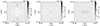Fig. 4. Comparison of the level populations throughout the simulated core shown in Fig. 3, under LTE conditions. When the level populations are designated without a second subscript to denote the magnetic quantum number all sublevel populations are degenerate. In the opposite case, the magnetic sublevels are explicitly considered in the detailed balance equations. As was expected, under LTE conditions, the numerical result is n0, 0 = n0 and $n_{1,0}=n_{1,\pm 1}=\frac{1}{3}{n}_1$, irrespective of the local physical conditions. Note that the differences are in units of 10−16.

In Fig. 5 we show spectra in antenna temperature units from the center of the core computed for each of the two cases described above. With the solid black line we show the spectrum when the magnetic-sublevel populations are degenerate. With the dash-dotted red and dotted blue lines we show, respectively, the spectra polarized perpendicular and parallel to the magnetic field. As was expected, under LTE conditions, I_total/2 = I_⊥ = I_∥. Additionally, the polarization fraction defined as

$$\begin{array}{c}\hfill p=\frac{I_{\perp }-I_{\Vert }}{I_{\perp }+I_{\Vert }-B}\end{array}$$(18)

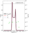Fig. 5. Comparison of the spectrum (in antenna temperature units) computed when the magnetic-sublevel populations are degenerate (solid black line) under LTE conditions, with the spectra polarized perpendicular and parallel to the magnetic field (dash-dotted red and dotted blue lines, respectively), computed when the magnetic sublevels are explicitly considered in the detailed balance equations. All spectra are from the central cell (R = Z = 0). The green points show the polarization fraction (right y axis). With the dashed black line we mark a lenient detection limit of 0.1% polarization. As was expected, under LTE conditions, I⊥ = I∥ = Itotal/2 and the polarization fraction is zero to numerical accuracy (note that the right y axis is in logarithmic scale spanning twenty-one orders of magnitude). The underlying physical model used for these radiative-transfer simulations is shown in Fig. 3.

is plotted with green squares with values corresponding to the right y axis. Any spurious polarization because of numerical noise is ≲10⁻¹⁴% or, in other words, thirteen orders of magnitude less than a lenient detection limit of 0.1% polarization.

3.2. Multilevel molecule under local thermodynamic equilibrium

Here, we extend the calculations performed in the previous section for a multilevel molecule with four rotational energy levels (J = 0 − 3). For four rotational levels, we need to compute the level populations for ten magnetic sublevels. Similarly to the previous section, the contribution from the CMB is considered in our calculations of the level populations.

In the left panel of Fig. 6 we show the population fraction of the different magnetic sublevels at the center of the core. As was expected, under LTE conditions, the magnetic sublevels of the same rotational levels have equal level populations. In the right panel of Fig. 6 we show the spectra from the CO J = 1 → 0 (solid lines), J = 2 → 1 (dashed lines) and J = 3 → 2 (dash-dotted) transitions. With the black lines we show the intensity polarized perpendicular to the magnetic field and with the red lines we show the intensity polarized parallel to the magnetic field. Here, we also show the polarization fraction from each transition, which once again is zero to numerical accuracy.

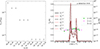Fig. 6. Our results for a multilevel molecule under LTE conditions. Left panel: Population fraction of the different magnetic sublevels at the center of the core (r = z = 0) under LTE conditions. Similarly to the two-level approximation, the level populations of the magnetic sublevels of the same rotational level are equal under LTE conditions. Right panel: Spectra of the different transitions toward the center of the cloud (i.e., R = Z = 0) and the corresponding polarization fraction (right y axis; see legends for the definition of the different linestyles and colors). Once again, any spurious polarization for any pair of rotational transitions is zero to numerical accuracy. The underlying physical model used for these radiative-transfer simulations is shown in Fig. 3.

3.3. Two-level molecule under non-local thermodynamic equilibrium

Now that we have established that no spurious linear polarization is present in our implementation, we proceed to test whether the numerical results for the polarization fraction under non-LTE conditions are in agreement with theoretical expectations. To do so, we compare the numerical result for the fractional polarization at the rest frequency of the line (ν_J, J′) with the analytical results of Kylafis (1983) for the polarization fraction as a function of the “mean” optical depth for 1D and 2D velocity fields.

For these numerical tests, we match the physical conditions as well as the Einstein A and collisional coefficients adopted by Kylafis (1983). Specifically, for the 1D velocity field, the only non-zero velocity component is taken to be along the magnetic-field direction with the velocity gradient being set equal to Λ₃ = 10⁻¹¹ s⁻¹. In the directions perpendicular to the field the cloud is taken to be infinite or, in other words, the optical depths are set to infinity. For the 2D velocity-field test, we set the velocity gradient in the directions perpendicular to the magnetic field equal to Λ₁ = Λ₂ = 10⁻⁹ s⁻¹, Λ₃ is equal to zero, and the optical depth along the magnetic-field direction is infinity. The physical models used are schematically shown in Fig. 7. These analytical models were implemented in a Cartesian discretized grid consisting by 8³ cells. However, we note that given the nature of the setup (LVG approximation) these calculations are by definition independent of the resolution. That is, these calculations could have been single-cell calculations (i.e., similarly to the original calculations presented in Goldreich & Kylafis 1981).

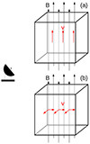Fig. 7. Schematic representation of the physical models used to compare our numerical results against analytical solutions and against previous calculations (see Sects. 3.3 and 3.4). In the upper panel the velocity field is set along magnetic-field lines and has a constant gradient of Λ3 = 10−11 s−1. In the lower panel the velocity field is perpendicular to magnetic field lines and the velocity gradient in each direction is Λ1 = Λ2 = 10−9 s−1.

In both these tests, the collisional and Einstein A coefficients are set equal to 9.4 × 10⁻¹² cm³ s⁻¹ and 1.8 × 10⁻⁷ s⁻¹, respectively, and the H₂ number density is set equal to 1.9 × 10⁴ cm⁻³, such that Cn_H2/A is equal to one. For the rest frequency of the CO (J = 1 → 0) line we adopt ν_J, J′ = 115.3 GHz (see also Table 1). Finally in both these test cases, the temperature is set equal to 30 K everywhere in our simulation grid and the contribution from the CMB in Eq. (2) is ignored, as in the study by Kylafis (1983). The LOS direction in both cases is perpendicular to the magnetic field such that the amount of polarization is maximum for the specific physical conditions under consideration.

For the 2D-velocity field we also compare our calculations with the numerical results obtained by Goldreich & Kylafis (1981) and Lankhaar & Vlemmings (2020a). For this comparison we adopt a temperature of T = 10 K and a number density of ∼4 × 10³ cm⁻³, such that Cn_H2/A = 0.212. Additionally, for this particular comparison alone we adopt, ν_J, J′ = 100 GHz, as is also the case in these two studies.

In the upper panel of Fig. 8 we show the polarization fraction at the rest frequency of the line as a function of the “mean” optical depth TAU, defined in Appendix B of Kylafis (1983) as

$$\begin{array}{c}\hfill \frac{1}{\mathrm{TAU}}={\displaystyle \int \frac{\mathrm{d}\mathrm{\Omega }}{4\pi }}\frac{1}{\tau }=\frac{1}{3{\tau }_0},\end{array}$$(19)

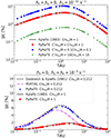Fig. 8. Polarization fraction as a function of the “mean” optical depth (see Sect. 3.3) for 1D (upper panel) and 2D (lower panel) velocity fields. A schematic representation of the physical models used is shown in Fig. 7. Upper panel: The solid black line shows the analytical results by Kylafis (1983) for CnH2/A = 1 and red squares show our numerical results for the same value of CnH2/A and with $C{\prime }_{m\to m\prime }=C_{J,m\to J\prime ,m\prime }$. Green stars and blue circles show our numerical results when we alter the value of $C{\prime }_{m\to m\prime }$ a factor of ten above and below CJ, m → J′, m′. Lower panel: The dashed black and dash-dotted magenta lines show the results from Goldreich & Kylafis (1981) and Lankhaar & Vlemmings (2020a) for CnH2/A = 0.212 and T = 10 K, and blue triangles show results obtained with PYRATE for the same values of CnH2/A and T. Finally, the solid black line and red squares show, respectively, the analytical results by Kylafis (1983) and $P\mathrm{Y}R\mathrm{A}TE\text{'}\mathrm{S}$ results for CnH2/A = 1 and T = 30 K.

where τ is the optical depth as a function of direction and

$$\begin{array}{c}\hfill {\tau }_0=\frac{3}{8\pi }(\frac{c}{{\nu }_{J,J\prime }}{)}^3{A}_{J,m\to J\prime ,m\prime }\frac{n_0-\frac{2n_{1,\pm 1}+n_{1,0}}{3}}{\mathrm{\Lambda }}.\end{array}$$(20)

where, in turn, Λ is the velocity gradient.

With red squares we plot our numerical results for Cn_H2/A = 1 and the solid black line shows the analytical results for the same value of Cn_H2/A. As is evident, the numerical results follow very well the analytical solution across all values of the “mean” optical depth. Finally, with blue circles and green stars in Fig. 8 we show our numerical results when Cn_H2/A = 1 but with $C{\prime }_{m\to m\prime }=0.1\times C_{J,m\to J\prime ,m\prime }$ and $C{\prime }_{m\to m\prime }=10\times C_{J,m\to J\prime ,m\prime }$, respectively. Increasing or decreasing the collisional coefficient between magnetic sublevels by a factor of ten leads to a significant decrease or increase in the polarization fraction. This is to be expected, as collisions tend to populate different sublevels equally and therefore the polarization fraction is inversely correlated to $C{\prime }_{m\to m\prime }$. However, as is evident from Fig. 8, the effect is non-linear. That is, decreasing the value of $C{\prime }_{m\to m\prime }$ leads to an increase in the polarization fraction by a factor of ∼3, whereas increasing the value of $C{\prime }_{m\to m\prime }$ by the same factor has a more dramatic effect and leads to a decrease in the polarization fraction by almost an order of magnitude.

In the bottom panel of Fig. 8 we show the polarization fraction at the rest frequency of the line for a 2D velocity field. The “mean” optical depth TAU is now defined as

$$\begin{array}{c}\hfill \frac{1}{\mathrm{TAU}}={\displaystyle \int \frac{d\mathrm{\Omega }}{4\pi }}\frac{1}{\tau }=\frac{2}{3{\tau }_0},\end{array}$$(21)

where τ₀ is once again given by Eq. (20). With the solid black line we show again the analytical results by Kylafis (1983) and with the red squares we plot our numerical results for the same setup. Once again, our calculations follow the analytical results very closely. Finally, with the dashed black and dash-dotted magenta lines we show, respectively, the numerical calculations by Goldreich & Kylafis (1981) and Lankhaar & Vlemmings (2020a) for the physical setup first considered in Goldreich & Kylafis (1981) and described above. We overplot our results with blue triangles. In contrast to PORTAL, our calculations follow the numerical results obtained by Goldreich & Kylafis (1981) very closely across the entire range of optical depths. We note, however, that for higher values of Cn_H2/A the error in PORTAL is reduced relative to the original findings by Goldreich & Kylafis (1981) (see Fig. 8 by Lankhaar & Vlemmings 2020a).

3.4. Multilevel molecule under non-local thermodynamic equilibrium

We now explore how the polarization fraction is affected when multiple rotational levels are considered in our calculations. To this end, we consider a total of four rotational levels (J = 0 − 3). The underlying physical model for the calculations presented here is identical to the one considered in the previous section for a 1D velocity field and is schematically shown in the upper panel of Fig. 7 (i.e., Λ₁ = Λ₂ = 0 and Λ₃ = 10⁻¹¹ s⁻¹). However, we now adopt again the collisional and Einstein coefficients from the LAMBDA database (Schöier et al. 2005). The value of the H₂ number density is set equal to 2.1 × 10²/10³/10⁴ cm⁻³, such that Cn_H2/A is 0.1, 1 and 10, respectively. Finally, the value of $C{\prime }_{m\to m\prime }$ is set equal to C_{J, m → J′, m′}. As in the previous numerical experiment the contribution from the CMB is not taken into account when computing the population densities of the different sublevels.

In Fig. 9 we show the polarization fraction from CO J = 1 → 0 transition in the two-level and multilevel cases for the three different values of Cn_H2/A. The black points show our calculations for the two-level case and the red points when considering multiple rotational levels. With triangles we show our results for Cn_H2/A = 10, with stars we show our results for Cn_H2/A = 1 and finally with the squares we show our results for Cn_H2/A = 0.1. Blue hexagons show a multilevel case with Cn_H2/A = 1. However, in this numerical test, only the radiative processes between the first two levels are taken into account whereas collisional processes are considered between all sublevels.

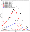Fig. 9. Polarization fraction as a function of the “mean" optical depth for different values of CnH2/A for the multilevel and two-level cases (red and black points, respectively). With triangles, stars and squares we show the polarization fraction for CnH2/A = 10, 1 and 0.1, respectively. With blue hexagons we show a multilevel case with CnH2/A = 1 where we only consider the radiative processes between levels J = 1 → 0 (collisional processes are considered between all sublevels). A schematic representation of the physical model used for these radiative-transfer simulations is shown in panel (a) of Fig. 7.

As is evident from Fig. 9, considering more rotational levels has a non-trivial effect in the fractional polarization. Specifically, when considering multiple levels, the peak in polarization fraction is observed at smaller “mean” optical depths. This is mostly evident in the case when Cn_H2/A = 1 whereas for Cn_H2/A= 10 and 0.1 the peak in polarization fraction is for “mean” optical depths close to unity, as in the two-level case. Upon closer inspection we found that this shift for the Cn_H2/A = 1 case is due to the fact that the factor n_1, 0 − n_1, ±1, to which the polarization fraction is proportional (e.g., Eq. (23) in Kylafis 1983), peaks at smaller “mean” optical depths. This shift is in turn caused by a change in the relative importance of the optical depths of the J = 1 → 0 and J = 2 → 1 transitions. To demonstrate this we ignore all radiative processes for all transitions with J ≥ 2 whereas collisional processes are normally taken into account between all sublevels (blue hexagons in Fig. 9). As was expected, the peak in polarization is again at “mean” optical depths of ∼1. Additionally, the polarization fraction is smaller compared to the multilevel case where all radiative processes are taken into account. This is due to the fact that the degeneracy between levels n_1, 0 and n_1, ±1 is broken exclusively by ℛ_1 → 0 and 𝒰_1 → 0 without additional contributions by ℛ_2 → 1 and 𝒰_2 → 1 (and indirect contributions by ℛ_3 → 2, 𝒰_3 → 2). Finally, in the case shown with blue hexagons in Fig. 9, the polarization fraction is smaller compared to the two-level case. This is also to be expected given the additional collisional quenching because of the higher rotational levels. A very similar trend was also obtained by Deguchi & Watson (1984) although the exact value of the polarization fraction predicted here differs from theirs for the same values of Cn_H2/A.

We should note however that there are a number of differences between the numerical calculations presented here and the calculations by Deguchi & Watson (1984). Firstly, as was noted in Sect. 2, we use Eq. (11) instead of Eq. (10) for computing the value of the Einstein A coefficient between all transitions (J, m)→(J′,m′). Additionally, Deguchi & Watson (1984) ignore collisions between magnetic sublevels whereas such interactions are taken into account for the results presented in Fig. 9. Thirdly, for the collisional coefficients C_{J, m → J′, m′}, Deguchi & Watson (1984) adopt their values from Green & Chapman (1978), which differ from the values used here by ∼30%. Moreover, the “mean” optical depth in Deguchi & Watson (1984) is defined only along the direction of the velocity gradient. Finally, as Deguchi & Watson (1984) do not explicitly quote the values they use for the Einstein A_{J → J′} coefficients, a one-to-one comparison between the different implementations is unfortunately not possible⁶.

4. Linear polarization in a prestellar core

In this section, we present radiative-transfer simulations of linear polarization of CO under non-LTE conditions for the physical model shown in Fig. 3, considering four rotational energy levels. The use of a nonideal MHD chemo-dynamical simulation enables us to have more realistic physical and chemical conditions for our radiative-transfer calculations. The contribution from the CMB is taken into account when computing the population densities and $C{\prime }_{m\to m\prime }$ is set equal to C_{J, m → J′, m′}. Finally, the core is observed edge-on, such that the mean component of the magnetic field is perpendicular to the line of sight and the fractional polarization is maximum.

In Figs. 10 and 11 we present our results from our numerical calculations for the J = 1 → 0 and J = 3 → 2 transitions. Results for the J = 2 → 1 transition are qualitatively very similar to the J = 1 → 0 transition and are therefore not shown here. In the upper row we show (in units of antenna temperature) the intensity of the line (I_total = I_⊥ + I_∥) in three different slices through our synthetic Position-Position-Velocity (PPV) data cube. The red contours show the actual density structure of the core (see Fig. 3). The velocity of these slices is marked with the dashed blue lines in the bottom row, where we additionally show a spectrum through the center of the core. Finally, in the middle row we show the fractional polarization in the entire core for each velocity slice. The radiative-radiative transfer results presented in Figs. 10 and 11 are converged with respect to the resolution of the underlying chemo-dynamical simulation used as input. Specifically, we considered two different resolutions (128 × 128 and 256 × 256; see Appendix B for our convergence test) in the underlying physical model used as input and found practically identical outcomes.

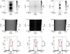Fig. 10. Results from our radiative-transfer simulation for the J = 1 → 0 transition for the chemo-dynamical simulation shown in Fig. 3. Upper row: Slices through the simulated PPV data cube for the velocities marked with the dashed blue lines in the lower row where we additionally show spectra at the center of the core. In each panel we have overplotted the actual density structure of the core with red contours. Middle row: Fractional polarization in each velocity slice. Bottom row: Spectra toward the center of the core (see blue point in the upper left panel; R = Z = 0) together with the polarization fraction (black squares) for this location in the cloud. With the black line we show the radiation polarized perpendicular to the magnetic field and with the red line we show the radiation polarized parallel to the magnetic field. For the physical conditions of the cloud shown in Fig. 3 the maximum fractional polarization is observed for the rest frequency of the line (middle panel in the second row).

Fig. 11. Same as Fig. 10 but for the J = 3 → 2 transition.

As was expected, the fractional polarization is maximum at the rest frequency for both the J = 1 → 0 and the J = 3 → 2 transitions. Specifically, for the J = 1 → 0 transition the polarization fraction is on the order of ∼1.5%, whereas for the J = 3 → 2 transition the polarization fraction toward the middle of the cloud is an order of magnitude less. Given the Einstein A and collisional coefficients, the factor Cn_H2/A for the J = 3 → 2 transition remains close to unity even in the inner regions of the cloud as opposed to the J = 1 → 0 transition where it reaches a maximum value of ∼24. Hence, the fact that the polarization fraction is higher for the J = 1 → 0 might at first seem counter-intuitive. However, the J = 3 → 2 transition is more optically thick with typical values of the optical depth being at an excess of 200. Therefore, a lower fractional polarization is to be expected especially considering that in the multilevel case the peak in polarization fraction is found at slightly smaller optical depths than the two-level case (see Fig. 9). As a result, in neither of the two transitions the polarized radiation comes from the inner regions of the core, but for (mostly) different physical reasons, which are further explained below.

Spatially, a small drop in the polarization fraction is observed toward the axis of symmetry of the cloud for the J = 1 → 0 transition (from 1.5% to 1.2%; see middle panel in the second row in Fig. 10). This drop in polarization fraction is a combined effect of two factors. Firstly, the H₂ number density increases near the axis of symmetry and consequently Cn_H2/A increases, leading to a decrease in polarization fraction. Secondly, and most importantly, the optical depth increases near the axis of symmetry leading to a further decrease in polarization fraction. This can be intuitively understood given the fact that photons emitted from regions of the cloud close to the axis of symmetry need to travel a longer distance. In contrast to the J = 1 → 0 transition, the polarization fraction in the J = 3 → 2 transition remains relatively uniform in the inner regions of the cloud and only increases to observationally detectable values toward the outer regions of the core, where both Cn_H2/A and the optical depth are low.

At the rest frequency of the J = 1 → 0 transition, the polarization fraction is positive through the entire core and only becomes negative in the outer regions of the core for frequencies close to ∼one thermal linewidth away from the rest frequency (left and right panels in the second row of Fig. 10). This implies that, at the rest frequency of this transition, the polarization is perpendicular to the magnetic field, but changes to being parallel in the outer regions of the core for other velocity slices. The same is largely true for the J = 3 → 2 transition. However, in this case the polarization becomes parallel to the magnetic field (negative polarization fraction) even for the rest frequency of the line and for |z|≳0.65 pc (middle panel in the second row of Fig. 11). Such differences in the polarization direction occur because the factor τ_J′,J^⊥ − τ_J′,J^∥ changes sign in these regions of the cloud. While changes in polarization direction between different transitions of the same molecule (and for the same region of the cloud) have been previously pointed out in the literature (e.g., Cortes et al. 2005), not much attention has been paid to variations in the polarization direction for the same transition. However, such variations have potentially been observed. For instance, Lai et al. (2003) found that CO and dust polarization vectors where aligned in one region of DR21(OH), whereas they were perpendicular in another region (see their Fig. 1). Such observed variations in the polarization direction, which can occur both between different transitions and within the same transition, may offer new insights in relation to the physical conditions inside molecular clouds. Specifically, in combination with dust polarization observations and numerical simulations (e.g., Bino et al. 2022), such variations in the polarization direction can reveal how the factor τ_J′,J^⊥ − τ_J′,J^∥ changes sign within different regions of the cloud. If so, such variations could potentially be used to probe the velocity component on the plane of the sky.

5. Summary and conclusions

We implemented a multilevel treatment of linear polarization of spectral lines due to an anisotropic radiation field in the multilevel non-LTE line radiative-transfer code PYRATE, a very well-known effect in physics and astrophysics since many decades. Different modes of polarized radiation are treated individually. The theoretical formalism followed was that developed by Deguchi & Watson (1984), which is strictly valid for a uniform magnetic field and when the magnetic precession rate exceeds the collisional and radiative rates. A radiative-transfer code that can model linear polarization of spectral lines when this condition is not satisfied is PORTA (Štěpán & Trujillo Bueno 2013), which uses the more general theoretical formalism by Landi Degl’Innocenti & Landolfi (2004).

We tested our implementation for various limiting cases and compared our numerical calculations against analytical results. Firstly, we confirmed that under LTE conditions the fractional polarization is zero to numerical accuracy, in both the two-level and multilevel cases. Additionally, we confirmed that even when the magnetic sublevels are explicitly considered, under LTE conditions, our results are identical to the case where the magnetic-sublevel populations are degenerate. We then compared our numerical calculations for the fractional polarization as a function of the “mean” optical depth against analytical results and found an excellent agreement.

Finally, we presented radiative-transfer simulations of linear polarization of CO (J = 1 → 0 and J = 3 → 2 transitions) using as input a chemo-dynamical, nonideal MHD simulation of a prestellar core when the central number density of the cloud is n_H2 = 5 × 10⁴ cm⁻³. At the rest frequency of the transitions, we found a relatively uniform polarization fraction throughout the inner regions of the cloud on the order of 1.5% and 0.15%, respectively.

With our new implementation, we can provide observationally testable predictions for the polarization fraction for any set of given physical parameters. Such predictions include the variation in the polarization fraction both spatially within an interstellar cloud and as a function of velocity. This synergy between simulations and observations can open new pathways for studying magnetic fields in various stages during the star formation process as well as potentially revealing the previously inaccessible POS component of the velocity field during the early stages in the star formation process.

Data availability

The code is freely available to download at https://github.com/ArisTr/PyRaTE.git.

Acknowledgments

We thank the anonymous referee for suggestions that improved this manuscript. We are also grateful to K. Tassis for useful comments. A. Tritsis acknowledges support by the Ambizione grant no. PZ00P2_202199 of the Swiss National Science Foundation (SNSF). The software used in this work was in part developed by the DOE NNSA-ASC OASCR Flash Center at the University of Chicago. We also acknowledge use of the following software: MATPLOTLIB (Hunter 2007), NUMPY (Harris et al. 2020), SCIPY (Virtanen et al. 2020), NUMBA (Lam et al. 2015), and the YT analysis toolkit (Turk et al. 2011).

References

Appendix A: Statistical equilibrium equations

Below, we provide the statistical equilibrium equations that describe the interactions between all magnetic sublevels for a system with an arbitrary number of rotational levels N

$$\begin{array}{c}\hfill {\displaystyle \sum _{J=0}^N\sum _{m=0}^J}{g}_{J,m}{n}_{J,m}-n_{\text{tot}}=0\end{array}$$(A.1a)

$$\begin{array}{cc}& \frac{d{n}_{J,m}}{\mathit{dt}}=0={\displaystyle \sum _{m^{\prime }=m-1}^{m+1}}\frac{g_{J+1,m^{\prime }}}{g_{J,m}}{A}_{J+1,m^{\prime }\to J,m}{n}_{J+1,m^{\prime }}-n_{J,m}{\displaystyle \sum _{m^{\prime }=m-1}^{m+1}}f(\mathrm{\Delta }g)A_{J,m\to J-1,m^{\prime }}+n_{{\mathrm{H}}_2}({\displaystyle \sum _{J^{\prime }>J}\sum _{m^{=}0}^{J^{\prime }}}{g}_{J^{\prime },m^{\prime }}{C}_{J^{\prime },m^{\prime }\to J,m}(n_{J^{\prime },m^{\prime }}-n_{J,m}{e}^{-\mathrm{\Delta }E/k_{B}T})\hfill \\ \hfill & +{\displaystyle \sum _{J^{\prime }<J}\sum _{m^{=}0}^{J^{\prime }}}{g}_{J^{\prime },m^{\prime }}{C}_{J^{\prime },m^{\prime }\to J,m}(n_{J^{\prime },m^{\prime }}{e}^{-\mathrm{\Delta }E/k_{B}T}-n_{J,m})+{\displaystyle \sum _{m^{\prime }\ne m}}{g}_{m^{\prime }}{C}_{m^{\prime }\to m}^{\prime }(n_{J,m^{\prime }}-n_{J,m}))+{\mathcal{R}}_{J+1\to J}(n_{J+1,m}-n_{J,m})-{\mathcal{R}}_{J\to J-1}(n_{J,m}-n_{J-1,m})\hfill \\ \hfill & +{\displaystyle \sum _{m^{\prime }\ne m}}\frac{g_{J+1,m^{\prime }}}{g_{J,m}}{\mathcal{U}}_{J+1\to J}(n_{J+1,m^{\prime }}-n_{J,m})-{\displaystyle \sum _{m^{\prime }\ne m}}\frac{g_{J-1,m^{\prime }}}{g_{J,m}}{\mathcal{U}}_{J\to J-1}(n_{J,m}-n_{J-1,m^{\prime }})\hfill \end{array}$$(A.1b)

where

$$\begin{array}{c}\hfill f(\mathrm{\Delta }g)=\{\begin{array}{cc}2,\hfill & \text{for}\mathrm{\Delta }g=1\hfill \\ \hfill \\ 1,\hfill & \text{otherwise},\hfill \end{array}\end{array}$$(A.2)

where, in turn, Δg = g_final − g_initial. In Eqs. (A.1a– A.1b) we have implicitly assumed that m and m′≥0.

Appendix B: Numerical Aspects

Here, we present the numerical aspects of our implementation along with the fundamental design logic of our algorithm. The code uses a ray-tracing approach to solve the radiative-transfer problem and an accelerated Λ-iteration to calculate the level populations. The polarized version of PYRATE can handle 2D cylindrical and 3D Cartesian uniform grids. Adaptive mesh refinement (AMR) grids are converted to uniform grids as described in Fig. 3 by Tritsis et al. (2018). To export results from AMR and uniform grids we use the YT analysis toolkit (Turk et al. 2011), which can handle the majority of the commonly used astrophysical MHD codes⁷. Spherical 1D grids are not supported by the polarized modules of PYRATE as this would imply ∇ ⋅ B ≠ 0. In fact, every spherically-symmetric system can be problematic to post-process in the context of the effect studied here as in the center of the cloud the velocity field would be isotropic and no polarization would occur.

In Fig. B.1 we show, in the form of a flow chart, the main design logic of PYRATE. Below, we outline key steps of the process followed.

1. We begin by exporting the physical parameters from a dynamical MHD simulation. Such parameters include n_H2, n_mol (the number density of the molecule in question), the three components of the velocity field, the three components of the magnetic field and the temperature in the simulation. Additionally, we read the frequency, collisional and Einstein coefficients from databases for molecular spectroscopy. At this stage, we also compute the collisional and Einstein coefficients between magnetic sublevels following Eqs. 11 & 12. The temperature dependence of the collisional coefficients is also stored in memory and used to interpolate the value of collisional coefficient inside each grid point. Finally, we read the values of the azimuthal and polar angles (ϕ_LOS, θ_LOS) under which the cloud is observed.

2. In order to compute the level populations in each grid point, we assume an initial optical depth in the x^±, y^±, z^±, secondary diagonal (“d_{xy, xz, yz}^±”) and anti-diagonal (“${\overline{d}}_{x\mathit{y},xz,\mathit{y}z}^{\pm }$”) directions for each polarization direction and pair of rotational levels, ${\tau }_{J\prime ,J}^{q,x^{\pm },{\mathit{y}}^{\pm },z^{\pm },d_{x\mathit{y},xz,\mathit{y}z}^{\pm },{\overline{d}}_{x\mathit{y},xz,\mathit{y}z}^{\pm }}$, along with an initial guess for the population densities. The initial values for the optical depths are such that the escape probabilities for each pair of levels and in every direction are equal to unity. Therefore, we essentially initialize the problem by assuming LTE conditions. The initial guess for the level populations (used as inputs to the MINPACK solver; see also point 4 below) is obtained by creating linearly spaced values based on the number of magnetic sublevels and the molecular number density in the grid point, while simultaneously ensuring that Eq. A.1a is satisfied. These initial guesses are utilized for the first grid point, while for subsequent grid points, the initial guesses are the solutions obtained at the preceding grid point.

3. Based on these initial guesses we numerically integrate Eqs. 1a & 1b. Integration is performed using the QUADPACK library (Piessens et al. 1983). Using the angles ϕ & θ passed to the integrating function in each integration step and the magnetic-field components in the grid point in question, we calculate the angle γ between the direction of propagation of radiation and the magnetic field. We then compute the optical depth toward that direction using Eq. 9 and subsequently the escape probability toward the same direction. Additionally, using the value for γ in each integration step and the guesses for the level populations we compute the source function and absorption coefficients following Eqs. 4 - 7.

4. With the values for the net radiative rates computed, we then solve Eqs. A.1. This system of non-linear equations is solved using the MINPACK library. The MINPACK library uses Powell’s hybrid method (Powell 1964), which is an iterative optimization algorithm. As such, step (3) is repeated for every iteration while solving Eqs.A.1.

5. Once the new values of n_J, m are computed for the first guess of the optical depths we proceed to update the values of ${\tau }_{J\prime ,J}^{q,x^{\pm },y^{\pm },z^{\pm },d_{xy,xz,yz}^{\pm },{\overline{d}}_{xy,xz,yz}^{\pm }}$. In order to take into account the change of the magnetic field direction along different sight-lines and in different regions of the cloud, we pre-compute the angles between the magnetic field in every grid point and the vectors $\widehat{{\mathit{w}}_{\mathit{n}}}$. These angles are used while calculating the absorption coefficients via Eqs. 4, which are then used to calculate ${\tau }_{J\prime ,J}^{q,x^{\pm },y^{\pm },z^{\pm },d_{xy,xz,yz}^{\pm },{\overline{d}}_{xy,xz,yz}^{\pm }}$ using Eqs. 8. The process (steps 3-5) continues until the level populations n_J, m simultaneously satisfy some tolerances. Additionally, in each new iteration “t + 2” during this Λ-iteration our new guess for n_J, m is $w_1{n}_{J,m}^{t+1}+w_2{n}_{J,m}^t$. For the values w₁ and w₂ we adopt 0.7 and 0.3, respectively (see also Fig. 2 in Tritsis et al. 2018 on the number of iterations required to converge using this accelerated Λ-iteration). The fact that our numerical scheme can reach the true self-consistent solution for the sublevel populations, and thus the polarization, is demonstrated by the fact that we match the analytical solutions by Kylafis (1983). However, by using our chemo-dynamical simulation, we verified that the same statement is also true for more complex non-LVG systems. Specifically, we performed two separate calculations (with four rotational levels) in which the magnetic sublevels were explicitly considered. In the first, we initialized the level populations from LTE conditions, and in the second, we initialized them using the non-LTE solution for the unpolarized case (e.g., see Fig. 2 and the discussion in Trujillo Bueno & Manso Sainz 1999). We found almost identical results (relative error < 10⁻⁷) regardless of how we initialized the sublevel populations.

6. Steps 2-5 are repeated for all grid points in our computation box or region, and the final values of the level populations are also stored for further use.

7. With the level populations computed we then define rays based on dx, dy, dz, x, y and z and the values for the polar and azimuthal angles. The case where the LOS coincides with one of the principal axes of the grid (say, for instance, the z axis) is trivial. In such a scenario the number and distance between rays is determined by dx and dy such that one ray passes through the center of each grid point on the “POS” face of the cube. If on the other hand the polar angle is such that rays pass diagonally through the grid (for simplicity the azimuthal angle is zero in this example), rays should begin at z_min − (x_max − x_min)/tanθ_LOS in order to ensure that rays are passing through the entire grid. Additionally, the distance between rays in the vertical POS axis should now be dz/sinθ_LOS in order not to distort the true dimensions of the grid. The distance traveled by each ray inside each grid point is then calculated by finding the intersection points of the unit vector of the rays (${\widehat{\mathit{w}}}_{\mathit{LOS}}$) with the faces of each cell. Finally, the LOS velocity component and the angle γ are calculated by a simple vector projection of v and B with ${\widehat{\mathit{w}}}_{\mathit{LOS}}$.

8. In the final step, for each ray and for each frequency, we compute the specific intensity or radiation polarized parallel and perpendicular to the field by integrating Eq. 13 for all grid points “k” along the LOS.

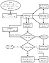Fig. B.1. Flow chart depicting the design logic of PYRATE. † Collisional coefficients are calculated according to Eq. 12. †† Einstein coefficients are calculated according to Eq. 11. ‡ Temperature dependence of collisional coefficients. The value of the collisional coefficient used in each grid point (i, j, k) is determined by interpolating based on TCJ → J′ and Ti, j, k. ¶ Integration is performed using the QUADPACK library (Piessens et al. 1983). The non-linear system of Eqs. A is solved using the MINPACK library (Moré et al. 1980).

The code is parallelized using openmpi and various functions are also accelerated using NUMBA (Lam et al. 2015) for better performance. To parallelize the code we use an “embarassingly parallel” technique (see also Fig. 4 from Tritsis et al. 2018) and as such the code is only partially parallelized in memory. For instance, when computing the level populations, each processor only handles part of the grid but still needs to have access over the entire arrays of velocity components in order to solve Eqs 8a & 8b. Consequently, given the number of data that need to be stored in memory, the code can easily handle 3D grids of up to 256³ in standard computing nodes whereas for larger grid sizes, large-memory nodes may be required, depending on the specific configuration and computing resources requested.

In Fig B.2 we present a convergence test for the radiative-transfer simulations presented in Fig. 10. For this test we use a simulation with the same initial and physical conditions as the simulation presented in Fig. 3 but with a factor of two higher base resolution (see Tritsis et al. 2022). Specifically, at the time of post-processing the resolution of the grid is 256×256. As is evident, the qualitative and quantitative behavior in both the total intensity and polarization fraction is very similar.

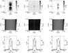Fig. B.2. Same as Fig. 10 but considering a higher resolution (by a factor of two) in the underlying physical model (shown in Fig. 3). The cyan line in the bottom row shows our results from Fig. 10.

Appendix C: Optical depth calculation

As was discussed in Sect. 2, in order to calculate the optical depth in each cell (i′,j′,k′) of our computational grid, we add the absorption coefficients from all cells (i, j, k) that fall within one thermal linewidth (see Eqs 8a & 8b). This is a physically driven choice for physical systems where the LVG is not valid, as photons emitted from one region of such a system will interact with another region that moves with approximately the same velocity. However, when adding the absorption coefficients of cells (i, j, k) we use an estimate for their level populations based on the molecular abundance in those cells and the level populations calculated in cell (i′,j′,k′). To demonstrate that this approach does not introduce errors, but it instead drastically improves the accuracy of the calculated level populations compared to the LVG case, we devise the following test for the unpolarized case. For the physical system shown in Fig. 3 (for which the LVG approximation is not valid) we start by calculating the optical depth in each cell based on the LVG approach; that is the optical depth is only subject to the local physical conditions within each cell. Based on this approach we obtain an “initial set of level populations” over the entire computational grid. We then re-iterate over the entire grid and re-calculate the optical depth in each cell (i′,j′,k′) this time considering all grid cells (i, j, k) that are one thermal linewidth away. For computing the absorption coefficient in cells (i, j, k) we consider their “initial set of level populations” from the previous iteration while the level populations and local optical depth in the cell of interest (i′,j′,k′) are allowed to change. We repeat the process, until we achieve convergence simultaneously over the entire grid. In this manner we essentially, consider the coupling between the level populations over the entire grid.

In Fig. C.1 we compare the population of the J = 0 level using this iterative approach (denoted as n₀′) against the population of the J = 0 level computed using the methodology described in Sect. 2. In the left panel, we show the ratio of the two populations (n₀′/n₀) after the first iteration over the entire grid (i.e., LVG-calculated optical depth), in the middle panel, we show the ratio after the second iteration, and in the right panel we show the ratio after the final iteration when the level populations of all rotational levels (J ≤ 5) over the entire grid have simultaneously converged (8 iterations with a relative tolerance of 10⁻³). As is evident from Fig. C.1, using the LVG optical depths leads to errors of more than 40% in the level populations. In contrast, the method described in Sect. 2 is accurate within 3%, while at the same time the code is ∼10 times faster.

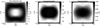Fig. C.1. Comparison between the population of J = 0 calculated using the approach described in Sect. 2 (n0) against the population of J = 0 calculated using the methodology described in Sect. C. In the latter case, the coupling between the level populations in different regions of the cloud is explicitly taken into account by performing multiple iterations over the entire grid. The method described in Sect. 2 is accurate within 3% while at the same time the code is ∼10 times faster. In both cases, we use as input the physical model shown in Fig. 3 and use J ≤ 5.

Finally, for a physical system with large enough velocity gradients Eqs 8a & 8b clearly reduce to the appropriate limit and the optical depths are calculated under the LVG approximation. That is, for such a system, the level populations in each cell will only depend on the local conditions within the cell and no other cells will be considered in the calculation of the optical depth since they will all be situated more than one thermal linewidth away.

Appendix D: Assessing errors for varying magnetic fields

As was already mentioned, the formalism presented in Sect. 2 is strictly valid for either an LVG system or for any system with a uniform magnetic field. To assess the errors introduced for non-LVG physical systems with varying magnetic fields along the LOS we perform the following numerical experiment. We utilize a 3D chemo-dynamical turbulent simulation of a molecular cloud (Tritsis; private communication), with an Alfvén Mach number of M_A = 1.2. As such, the magnetic field in each grid cell along the LOS is uncorrelated to the magnetic field inside every other grid cell along the LOS. We post-process this simulation using the polarized and unpolarized versions of PYRATE when the “central” number density is 5 × 10³ cm⁻³ and produce CO (J = 1 → 0) spectra, considering only two energy levels. We then compare our results for Stokes I between the polarized and unpolarized radiative-transfer calculations. The reasoning behind this experiment is that should significant errors were introduced, we should observe significant differences between Stokes I calculated using the two methods.

In Fig. D.1 we show spectra from four random different lines of sight (panels 1–4 from left to right). With the dash-dotted red lines we show I_⊥, with dotted blue lines we show I_∥ and with the solid black lines we show I_total/2 from our unpolarized radiative-transfer simulations. Finally, with the dashed magenta lines we show Stokes I/2 = (I_⊥ + I_∥)/2 from our polarized radiative-transfer simulations. As is demonstrated in Fig. D.1, I_⊥ + I_∥ is always in very good agreement with I_total. In fact, from all sight-lines and for all velocity channels in the interval [-0.9, 0.9] km s⁻¹ the relative error between I_total (unpolarized simulations) and I_⊥ + I_∥ (polarized simulations) does not exceed 0.2%. A distribution showing the relative error in Stokes I is shown in the fifth panel of Fig. D.1. The standard deviation of this distribution is ${\sigma }_{I_{\mathit{err}}^{\mathit{rel}}}$ is just 0.07 %, whereas the standard deviation of the distribution of absolute errors between I_total and I_⊥ + I_∥ is ${\sigma }_{I_{\mathit{err}}^{\mathit{abs}}}\approx 1\mathrm{mK}$. Finally, to assess the errors in polarization fraction, we perform the following calculation. We first add or subtract the difference between I_⊥ + I_∥ and I_total to or from I_⊥ and I_∥ assuming random weights w and 1 − w, respectively, with 0 ≤ w ≤ 1. We then calculate anew the value of the polarization fraction p′ based on these corrected values for I_⊥ and I_∥ and compute the relative error with respect to the initial value of the polarization fraction. The distribution of relative errors in polarization fraction is shown in the right panel of Fig. D.1 and its standard deviation is ∼13 %. Therefore, even in the case where the magnetic field of the underlying physical system is highly varying, the errors introduced by our formalism are marginal.

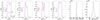Fig. D.1. The first four panels show a comparison between the Stokes I calculated using the unpolarized modules of PYRATE (Itotal; solid black lines) with Stokes I calculated as I⊥ + I∥ (dashed magenta, dash-dotted red and dotted blue lines, respectively) from radiative-transfer simulations of linear polarization for different lines of sight. In the fifth panel we show a distribution of relative errors between Itotal and I⊥ + I∥. The Stokes I between the two cases is nearly identical with only very minimal differences, indicating that no significant errors are introduced given our formalism, even for varying magnetic fields along the LOS. In the last panel we show a distribution of relative errors between the polarization fraction computed from I⊥ and I∥ and the polarization fraction (p′) after accounting for the “missing” or the “excess” specific intensity of radiation.

All Tables

All Figures

	Fig. 1. Schematic representation of all the processes considered for a molecular species with three rotational energy levels, when the magnetic sublevels are considered independently. Absorption and stimulated emission associated with Δm = 0 are marked with red, while the corresponding transitions associated with |Δm| = 1 are marked in green.
In the text

Fig. 2. Interpolated values of the optical depth inside a single cell, based on Eq. (9), along each direction $\widehat{\mathbf{\Omega }}$. In this example, the values of the optical depth in the directions x+, x−, y+, y−, $z^{+},z^{-},d_{x\mathit{y}}^{+},d_{x\mathit{y}}^{-},{\overline{d^{+}}}_{x\mathit{y}},{\overline{d^{-}}}_{x\mathit{y}},d_{\mathit{xz}}^{+},d_{\mathit{xz}}^{-},{\overline{d^{+}}}_{\mathit{xz}},{\overline{d^{-}}}_{\mathit{xz}},d_{\mathit{y}z}^{+},d_{\mathit{y}z}^{-},{\overline{d^{+}}}_{\mathit{y}z}$ and ${\overline{d^{-}}}_{\mathit{y}z}$ are equal to 14, 7, 6, 0.5, 7, 5, 2, 1.5, 5, 13, 9, 6, 9, 8, 4, 3, 10 and 3, respectively.

In the text

	Fig. 3. H2 and CO number densities (left and right panels, respectively) from a nonideal MHD chemo-dynamical simulation. Orange streamlines in the left panel depict the magnetic field lines and the color-coded vectors show the velocity in the cloud. This simulation is used as the underlying physical model in Sect. 3.1, Sect. 3.2, and Sect. 4.
In the text

Fig. 4. Comparison of the level populations throughout the simulated core shown in Fig. 3, under LTE conditions. When the level populations are designated without a second subscript to denote the magnetic quantum number all sublevel populations are degenerate. In the opposite case, the magnetic sublevels are explicitly considered in the detailed balance equations. As was expected, under LTE conditions, the numerical result is n0, 0 = n0 and $n_{1,0}=n_{1,\pm 1}=\frac{1}{3}{n}_1$, irrespective of the local physical conditions. Note that the differences are in units of 10−16.

In the text

Fig. 5. Comparison of the spectrum (in antenna temperature units) computed when the magnetic-sublevel populations are degenerate (solid black line) under LTE conditions, with the spectra polarized perpendicular and parallel to the magnetic field (dash-dotted red and dotted blue lines, respectively), computed when the magnetic sublevels are explicitly considered in the detailed balance equations. All spectra are from the central cell (R = Z = 0). The green points show the polarization fraction (right y axis). With the dashed black line we mark a lenient detection limit of 0.1% polarization. As was expected, under LTE conditions, I⊥ = I∥ = Itotal/2 and the polarization fraction is zero to numerical accuracy (note that the right y axis is in logarithmic scale spanning twenty-one orders of magnitude). The underlying physical model used for these radiative-transfer simulations is shown in Fig. 3.

In the text

Fig. 6. Our results for a multilevel molecule under LTE conditions. Left panel: Population fraction of the different magnetic sublevels at the center of the core (r = z = 0) under LTE conditions. Similarly to the two-level approximation, the level populations of the magnetic sublevels of the same rotational level are equal under LTE conditions. Right panel: Spectra of the different transitions toward the center of the cloud (i.e., R = Z = 0) and the corresponding polarization fraction (right y axis; see legends for the definition of the different linestyles and colors). Once again, any spurious polarization for any pair of rotational transitions is zero to numerical accuracy. The underlying physical model used for these radiative-transfer simulations is shown in Fig. 3.

In the text

Fig. 7. Schematic representation of the physical models used to compare our numerical results against analytical solutions and against previous calculations (see Sects. 3.3 and 3.4). In the upper panel the velocity field is set along magnetic-field lines and has a constant gradient of Λ3 = 10−11 s−1. In the lower panel the velocity field is perpendicular to magnetic field lines and the velocity gradient in each direction is Λ1 = Λ2 = 10−9 s−1.

In the text

Fig. 8. Polarization fraction as a function of the “mean” optical depth (see Sect. 3.3) for 1D (upper panel) and 2D (lower panel) velocity fields. A schematic representation of the physical models used is shown in Fig. 7. Upper panel: The solid black line shows the analytical results by Kylafis (1983) for CnH2/A = 1 and red squares show our numerical results for the same value of CnH2/A and with $C{\prime }_{m\to m\prime }=C_{J,m\to J\prime ,m\prime }$. Green stars and blue circles show our numerical results when we alter the value of $C{\prime }_{m\to m\prime }$ a factor of ten above and below CJ, m → J′, m′. Lower panel: The dashed black and dash-dotted magenta lines show the results from Goldreich & Kylafis (1981) and Lankhaar & Vlemmings (2020a) for CnH2/A = 0.212 and T = 10 K, and blue triangles show results obtained with PYRATE for the same values of CnH2/A and T. Finally, the solid black line and red squares show, respectively, the analytical results by Kylafis (1983) and $P\mathrm{Y}R\mathrm{A}TE\text{'}\mathrm{S}$ results for CnH2/A = 1 and T = 30 K.

In the text

Fig. 9. Polarization fraction as a function of the “mean" optical depth for different values of CnH2/A for the multilevel and two-level cases (red and black points, respectively). With triangles, stars and squares we show the polarization fraction for CnH2/A = 10, 1 and 0.1, respectively. With blue hexagons we show a multilevel case with CnH2/A = 1 where we only consider the radiative processes between levels J = 1 → 0 (collisional processes are considered between all sublevels). A schematic representation of the physical model used for these radiative-transfer simulations is shown in panel (a) of Fig. 7.

In the text

Fig. 10. Results from our radiative-transfer simulation for the J = 1 → 0 transition for the chemo-dynamical simulation shown in Fig. 3. Upper row: Slices through the simulated PPV data cube for the velocities marked with the dashed blue lines in the lower row where we additionally show spectra at the center of the core. In each panel we have overplotted the actual density structure of the core with red contours. Middle row: Fractional polarization in each velocity slice. Bottom row: Spectra toward the center of the core (see blue point in the upper left panel; R = Z = 0) together with the polarization fraction (black squares) for this location in the cloud. With the black line we show the radiation polarized perpendicular to the magnetic field and with the red line we show the radiation polarized parallel to the magnetic field. For the physical conditions of the cloud shown in Fig. 3 the maximum fractional polarization is observed for the rest frequency of the line (middle panel in the second row).

In the text

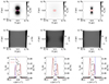	Fig. 11. Same as Fig. 10 but for the J = 3 → 2 transition.
In the text

Fig. B.1. Flow chart depicting the design logic of PYRATE. † Collisional coefficients are calculated according to Eq. 12. †† Einstein coefficients are calculated according to Eq. 11. ‡ Temperature dependence of collisional coefficients. The value of the collisional coefficient used in each grid point (i, j, k) is determined by interpolating based on TCJ → J′ and Ti, j, k. ¶ Integration is performed using the QUADPACK library (Piessens et al. 1983). The non-linear system of Eqs. A is solved using the MINPACK library (Moré et al. 1980).

In the text

	Fig. B.2. Same as Fig. 10 but considering a higher resolution (by a factor of two) in the underlying physical model (shown in Fig. 3). The cyan line in the bottom row shows our results from Fig. 10.
In the text

Fig. C.1. Comparison between the population of J = 0 calculated using the approach described in Sect. 2 (n0) against the population of J = 0 calculated using the methodology described in Sect. C. In the latter case, the coupling between the level populations in different regions of the cloud is explicitly taken into account by performing multiple iterations over the entire grid. The method described in Sect. 2 is accurate within 3% while at the same time the code is ∼10 times faster. In both cases, we use as input the physical model shown in Fig. 3 and use J ≤ 5.

In the text

Fig. D.1. The first four panels show a comparison between the Stokes I calculated using the unpolarized modules of PYRATE (Itotal; solid black lines) with Stokes I calculated as I⊥ + I∥ (dashed magenta, dash-dotted red and dotted blue lines, respectively) from radiative-transfer simulations of linear polarization for different lines of sight. In the fifth panel we show a distribution of relative errors between Itotal and I⊥ + I∥. The Stokes I between the two cases is nearly identical with only very minimal differences, indicating that no significant errors are introduced given our formalism, even for varying magnetic fields along the LOS. In the last panel we show a distribution of relative errors between the polarization fraction computed from I⊥ and I∥ and the polarization fraction (p′) after accounting for the “missing” or the “excess” specific intensity of radiation.

In the text

References

- Barnes, P. J., Ryder, S. D., Novak, G., et al. 2023, ApJ, 945, 34 [NASA ADS] [CrossRef] [Google Scholar]
- Bino, G., Basu, S., Machida, M. N., et al. 2022, ApJ, 936, 29 [NASA ADS] [CrossRef] [Google Scholar]
- Brinch, C., & Hogerheijde, M. R. 2010, A&A, 523, A25 [NASA ADS] [CrossRef] [EDP Sciences] [Google Scholar]
- Caselli, P., Walmsley, C. M., Terzieva, R., et al. 1998, ApJ, 499, 234 [NASA ADS] [CrossRef] [Google Scholar]
- Castor, J. I. 1970, MNRAS, 149, 111 [NASA ADS] [Google Scholar]
- Chandrasekhar, S., & Fermi, E. 1953, ApJ, 118, 113 [Google Scholar]
- Chapman, N. L., Goldsmith, P. F., Pineda, J. L., et al. 2011, ApJ, 741, 21 [NASA ADS] [CrossRef] [Google Scholar]
- Cortes, P. C., Crutcher, R. M., & Watson, W. D. 2005, ApJ, 628, 780 [NASA ADS] [CrossRef] [Google Scholar]
- Cortés, P. C., Sanhueza, P., Houde, M., et al. 2021, ApJ, 923, 204 [CrossRef] [Google Scholar]
- Crutcher, R. M., Hakobian, N., & Troland, T. H. 2009, ApJ, 692, 844 [NASA ADS] [CrossRef] [Google Scholar]
- Davis, L. 1951, Phys. Rev., 81, 890 [Google Scholar]
- Deguchi, S., & Watson, W. D. 1984, ApJ, 285, 126 [NASA ADS] [CrossRef] [Google Scholar]
- Deguchi, S., & Watson, W. D. 1990, ApJ, 354, 649 [NASA ADS] [CrossRef] [Google Scholar]
- de Jong, T., Boland, W., & Dalgarno, A. 1980, A&A, 91, 68 [NASA ADS] [Google Scholar]
- Falgarone, E., Troland, T. H., Crutcher, R. M., et al. 2008, A&A, 487, 247 [CrossRef] [EDP Sciences] [Google Scholar]
- Forbrich, J., Wiesemeyer, H., Thum, C., et al. 2008, A&A, 492, 757 [NASA ADS] [CrossRef] [EDP Sciences] [Google Scholar]
- Girart, J. M., Greaves, J. S., Crutcher, R. M., et al. 2004, Ap&SS, 292, 119 [NASA ADS] [CrossRef] [Google Scholar]
- Goldreich, P., & Kylafis, N. D. 1981, ApJ, 243, L75 [NASA ADS] [CrossRef] [Google Scholar]
- Goldreich, P., & Kylafis, N. D. 1982, ApJ, 253, 606 [NASA ADS] [CrossRef] [Google Scholar]
- Goldreich, P., Keeley, D. A., & Kwan, J. Y. 1973, ApJ, 179, 111 [NASA ADS] [CrossRef] [Google Scholar]
- Green, S., & Chapman, S. 1978, ApJS, 37, 169 [Google Scholar]
- Hanle, W. 1924, Z. Phys., 30, 93 [NASA ADS] [CrossRef] [Google Scholar]
- Happer, W. 1972, Rev. Mod. Phys., 44, 169 [NASA ADS] [CrossRef] [Google Scholar]
- Harris, C. R., Millman, K. J., van der Walt, S. J., et al. 2020, Nature, 585, 357 [NASA ADS] [CrossRef] [Google Scholar]
- Houde, M., Lankhaar, B., Rajabi, F., et al. 2022, MNRAS, 511, 295 [CrossRef] [Google Scholar]
- House, L. L. 1970, J. Quant. Spectr. Rad. Transf., 10, 1171 [NASA ADS] [CrossRef] [Google Scholar]
- Huang, K.-Y., Kemball, A. J., Vlemmings, W. H. T., et al. 2020, ApJ, 899, 152 [NASA ADS] [CrossRef] [Google Scholar]
- Hunter, J. D. 2007, Comput. Sci. Eng., 9, 90 [NASA ADS] [CrossRef] [Google Scholar]
- Kunz, M. W., & Mouschovias, T. C. 2010, MNRAS, 408, 322 [NASA ADS] [CrossRef] [Google Scholar]
- Kylafis, N. D. 1983, ApJ, 267, 137 [CrossRef] [Google Scholar]
- Lai, S.-P., Girart, J. M., & Crutcher, R. M. 2003, ApJ, 598, 392 [NASA ADS] [CrossRef] [Google Scholar]
- Lam, S. K., Pitrou, A., & Seibert, S. 2015, Numba: A LLVM-based Python JIT compiler. In Proceedings of the 2nd Workshop on the LLVM Compiler Infrastructure in HPC (LLVM’15) (New York, NY: ACM) [Google Scholar]
- Lamb, F. K., & Ter Haar, D. 1971, Phys. Rep., 2, 253 [NASA ADS] [CrossRef] [Google Scholar]
- Landi Degl’Innocenti, E. 1978, A&A, 66, 119 [Google Scholar]
- Landi Degl’Innocenti, E. 1983, Sol. Phys., 85, 33 [CrossRef] [Google Scholar]
- Landi Degl’Innocenti, E., & Landolfi, M. 2004, Polarization in Spectral Lines (Dordrecht: Kluwer Academic Publishers) [Google Scholar]
- Lankhaar, B., & Vlemmings, W. 2019, A&A, 628, A14 [NASA ADS] [CrossRef] [EDP Sciences] [Google Scholar]
- Lankhaar, B., & Vlemmings, W. 2020a, A&A, 636, A14 [NASA ADS] [CrossRef] [EDP Sciences] [Google Scholar]
- Lankhaar, B., & Vlemmings, W. 2020b, A&A, 638, L7 [NASA ADS] [CrossRef] [EDP Sciences] [Google Scholar]
- Lucy, L. B. 1971, ApJ, 163, 95 [Google Scholar]
- Meerts, W. L., De Leeuw, F. H., & Dymanus, A. 1977, CP, 22, 319 [NASA ADS] [Google Scholar]
- Mihalas, D. 1978, Stellar atmospheres (San Francisco: W.H. Freeman), 1978 [Google Scholar]
- Moré, J. J., Garbow, B. S., & Hillstrom, K. E. 1980, User Guide for MINPACK-1, Argonne National Laboratory Report ANL-80-74, Argonne, Ill [Google Scholar]
- Morris, M., Lucas, R., & Omont, A. 1985, A&A, 142, 107 [NASA ADS] [Google Scholar]
- Mouschovias, T. C., & Ciolek, G. E. 1999, The Origin of Stars and Planetary Systems, 540, 305 [NASA ADS] [CrossRef] [Google Scholar]
- Mouschovias, T. C., & Spitzer, L. 1976, ApJ, 210, 326 [NASA ADS] [CrossRef] [Google Scholar]
- Panopoulou, G. V., Psaradaki, I., & Tassis, K. 2016, MNRAS, 462, 1517 [Google Scholar]
- Piessens, R., de Doncker-Kapenga, E., & Ueberhuber, C. W. 1983, Springer Series in Computational Mathematics (Berlin: Springer), 1983 [Google Scholar]
- Powell, M. J. D. 1964, CompJ, 7, 155 [Google Scholar]
- Rasch, J., & Yu, A. C. H. 2003, SIAM J. Sci. Comput., 25, 1416 [Google Scholar]
- Schöier, F. L., van der Tak, F. F. S., van Dishoeck, E. F., et al. 2005, A&A, 432, 369 [Google Scholar]
- Skalidis, R., & Tassis, K. 2021, A&A, 647, A186 [NASA ADS] [CrossRef] [EDP Sciences] [Google Scholar]
- Sobolev, V. V. 1960, Moving Envelopes of Stars (Cambridge: Harvard University Press) [Google Scholar]
- Stenflo, J. O. 1994, Astrophys. Space Sci. Libr., 189 [Google Scholar]
- Stenflo, J. O., & Keller, C. U. 1997, A&A, 321, 927 [NASA ADS] [Google Scholar]
- Stenflo, J. O., Baur, T. G., & Elmore, D. F. 1980, A&A, 84, 60 [NASA ADS] [Google Scholar]
- Štěpán, J., & Trujillo Bueno, J. 2013, A&A, 557, A143 [NASA ADS] [CrossRef] [EDP Sciences] [Google Scholar]
- Townes, C. H., & Schawlow, A. L. 1955, Microwave Spectroscopy (New York: McGraw-Hill) [Google Scholar]
- Tritsis, A., Yorke, H., & Tassis, K. 2018, MNRAS, 478, 2056 [NASA ADS] [Google Scholar]
- Tritsis, A., Federrath, C., Willacy, K., et al. 2022, MNRAS, 510, 4420 [NASA ADS] [CrossRef] [Google Scholar]
- Tritsis, A., Basu, S., & Federrath, C. 2023, MNRAS, 521, 5087 [NASA ADS] [CrossRef] [Google Scholar]
- Troland, T. H., & Crutcher, R. M. 2008, ApJ, 680, 457 [NASA ADS] [CrossRef] [Google Scholar]
- Trujillo Bueno, J. 2001, ASP Conf. Ser., 236, 161 [Google Scholar]
- Trujillo Bueno, J., & del Pino Alemán, T. 2022, ARA&A, 60, 415 [NASA ADS] [CrossRef] [Google Scholar]
- Trujillo Bueno, J., & Manso Sainz, R. 1999, ApJ, 516, 436 [NASA ADS] [CrossRef] [Google Scholar]
- Turk, M. J., Smith, B. D., Oishi, J. S., et al. 2011, ApJS, 192, 9 [NASA ADS] [CrossRef] [Google Scholar]
- van der Tak, F. F. S., Black, J. H., Schöier, F. L., et al. 2007, A&A, 468, 627 [NASA ADS] [CrossRef] [EDP Sciences] [Google Scholar]
- Virtanen, P., Gommers, R., Oliphant, T. E., et al. 2020, Nat. Methods, 17, 261 [Google Scholar]
- Ward-Thompson, D., Pattle, K., Bastien, P., et al. 2017, ApJ, 842, 66 [Google Scholar]
- Yang, L., & Lai, S. P. 2010, JTAM, ASRROC 2010 Symposium Proceedings: Probing the magnetic field structure in star-forming regions through molecular line polarization, 8 [Google Scholar]