| Issue |
A&A
Volume 691, November 2024
|
|
|---|---|---|
| Article Number | A204 | |
| Number of page(s) | 10 | |
| Section | Galactic structure, stellar clusters and populations | |
| DOI | https://doi.org/10.1051/0004-6361/202452064 | |
| Published online | 13 November 2024 | |
Evolution of the mass-radius relation of expanding very young star clusters
1
Max-Planck-Institut für Radioastronomie,
Auf dem Hügel 69,
53121
Bonn,
Germany
2
Helmholtz-Institut für Strahlen- und Kernphysik (HISKP), Universität Bonn,
Nussallee 14–16,
53115
Bonn,
Germany
3
Charles University in Prague, Faculty of Mathematics and Physics, Astronomical Institute,
V Holešovičkách 2,
180 00
Praha 8,
Czech Republic
★ Corresponding author; This email address is being protected from spambots. You need JavaScript enabled to view it.
; This email address is being protected from spambots. You need JavaScript enabled to view it.
Received:
30
August
2024
Accepted:
30
September
2024
Abstract
The initial mass–radius relation of embedded star clusters is an essential boundary condition for understanding the evolution of embedded clusters in which stars form to their release into the galactic field via an open star cluster phase. The initial mass–radius relation of embedded clusters deduced by Marks & Kroupa (2012, A&A, 543, A8) is significantly different from the relation suggested by Pfalzner et al. (2016, A&A, 586, A68). Here, we use direct N-body simulations to model the early expansion of embedded clusters after the expulsion of their residual gas. The observationally deduced radii of clusters up to a few million years old, compiled from various sources, are well fitted by N-body models, implying that these observed very young clusters are most likely in an expanding state. We show that the mass–radius relation of Pfalzner et al. (2016) reflects the expansion of embedded clusters following the initial mass–radius relation of Marks & Kroupa (2012). We also suggest that even the embedded clusters in ATLASGAL clumps with HII regions are probably already in expansion. All the clusters collected here from different observations show a mass-radius relation with a similar slope, which may indicate that all clusters were born with a profile resembling that of the Plummer phase-space distribution function.
Key words: stars: evolution / galaxies: star clusters: general / galaxies: star formation
© The Authors 2024
 Open Access article, published by EDP Sciences, under the terms of the Creative Commons Attribution License (https://creativecommons.org/licenses/by/4.0), which permits unrestricted use, distribution, and reproduction in any medium, provided the original work is properly cited.
This article is published in open access under the Subscribe to Open model.
Open Access funding provided by Max Planck Society.
1 Introduction
The formation of stars within molecular clouds and the early stages of stellar evolution are active research topics. Most, and perhaps even all, of the observed stars were formed in embedded clusters (Kroupa 1995a,b; Lada & Lada 2003; Kroupa 2005; Megeath et al. 2016; Dinnbier et al. 2022). The central hub of a hub-filament system in molecular cloud could serve as the precursor of an embedded cluster. In hub-filament systems, converging flows are funneling matter into the hub through the filaments, such that cores embedded in the hub can prolong the accretion time for growing massive stars due to the sustained supply of matter (Myers 2009; Schneider et al. 2012; Peretto et al. 2013; Longmore et al. 2014; Motte et al. 2018; Vázquez-Semadeni et al. 2019; Kumar et al. 2020; Zhou et al. 2022). Ultimately the feedback energy from the protostars and pre-main sequence stars expels the remaining gas, and the embedded cluster expands. Therefore, measurements of the internal dynamics of young clusters and star-forming regions are necessary to fully understand the process of their formation and dynamical evolution.
Increasing observational evidence suggests that early expansion plays a fundamental role in the dynamical evolution of young star clusters. A useful visualization of the expansion of real star clusters is provided by the collation in Fig. 4 of Brandner (2008). Gaia DR2 and DR3 data have opened a new window onto the internal kinematics of young star clusters and large star-forming complexes. Several case studies based on Gaia DR2 and DR3 data and multi-object spectroscopy have revealed the expansion of very young clusters in star-forming regions (Wright et al. 2019; Cantat-Gaudin et al. 2019; Kuhn et al. 2020; Lim et al. 2020; Swiggum et al. 2021; Lim et al. 2022; Mužić et al. 2022; Das et al. 2023; Flaccomio et al. 2023; Jadhav et al. 2024). Statistically, in Kuhn et al. (2019), for 28 clusters and associations with ages of about 1–5 Myr, proper motions from Gaia DR2 reveal that at least 75% of these systems are expanding. Della Croce et al. (2023) presented a comprehensive kinematic analysis of almost all known young (t < 300 Myr) Galactic clusters based on the improved astrometric quality of the Gaia DR3 data, finding that a remarkable fraction (up to 80%) of clusters younger than ≈30 Myr are currently experiencing significant expansion. Wright et al. (2023) presented a large-scale 3D kinematic study of ≈2000 spectroscopically confirmed young stars (t < 20 Myr) in 18 star clusters and OB associations (groups) from the combination of Gaia astrometry and Gaia-ESO Survey spectroscopy, showing that nearly all of the groups studied are in the process of expansion.
Bastian & Goodwin (2006) compared the luminosity profiles of young massive clusters, such as M82-F, NGC 1569-A, and NGC 1705-1, with N-body simulations of clusters that had experienced rapid gas expulsion, resulting in the loss of a substantial portion of their mass. They found the observed profiles to closely agree with the simulations. Goodwin & Bastian (2006) analyzed the differences between luminosity-based and dynamical mass estimates for young massive stellar clusters. Their results revealed significant discrepancies, which they attributed to the possibility that many young clusters are not in virial equilibrium due to undergoing violent relaxation following gas expulsion. Additionally, these authors noted that the increasing core radii observed in young clusters within the Large Magellanic Cloud and Small Magellanic Cloud can be well explained as an effect of rapid gas loss. In Kroupa et al. (2001) and Banerjee & Kroupa (2013, 2014, 2015), direct N -body modeling of realistic star clusters with a monolithically formed structure and undergoing residual gas expulsion consistently reproduced the characteristics of several well-observed very young star clusters, namely the Orion Nebula Cluster (ONC) and the clusters R136 and NGC 3603, thereby shedding light on the birth conditions of massive star clusters. Similar simulations were also carried out in Banerjee & Kroupa (2017) to explain how young massive star clusters attain their current shapes and sizes from an initially compact embedded morphology. These authors found that young massive clusters cannot expand to their current sizes if only two-body relaxation, stellar mass loss and dynamical heating through initial binaries are considered. They also confirmed that a substantial residual gas expulsion with ~30% star formation efficiency can adequately swell the newborn embedded clusters. The simulations of Banerjee & Kroupa (2013, 2014, 2015, 2017) start from an initially compact configuration of the computed cluster with the initial mass–radius relation of embedded clusters deduced by Marks & Kroupa (2012):
 (1)
(1)
This relation was derived from the radii and densities of open star clusters and the binding energy distributions of the surviving binary stars in them as these constrain the birth, or the initial half-mass radii, of the precursor embedded star clusters. Based on the universality of the early cluster expansion, in the present work, we collected various cluster samples to characterize the early cluster expansion using the numerical simulation recipes in Kroupa et al. (2001), Banerjee & Kroupa (2013, 2014, 2015) and Dinnbier et al. (2022), with our main goal being to study the evolution of the initial mass–radius relation of embedded clusters.
2 N-body simulations
2.1 Basic parameters
The parameters for the simulation were summarized from previous work, i.e. Kroupa et al. (2001); Baumgardt & Kroupa (2007); Banerjee et al. (2012); Banerjee & Kroupa (2013, 2014, 2015); Oh et al. (2015); Oh & Kroupa (2016); Banerjee & Kroupa (2017); Brinkmann et al. (2017); Oh & Kroupa (2018); Wang et al. (2019); Pavlik et al. (2019); Wang et al. (2020b); Dinnbier et al. (2022). The previous simulations have already demonstrated the effectiveness and rationality of these parameter settings (see below). The influence of different parameter settings on simulation results and the multidimensional parameter space are discussed in the aforementioned literature and their references. In the present work, we mainly use the mature simulation recipe to interpret observational data. With this contribution, we are not aiming to provide all possible solutions, as this would entail searching for solutions in a high-dimensional space (cluster mass, age, age spread, star formation efficiency, time of onset of gas expulsion, initial spatial configuration of the embedded cluster – spherical or not, and fractal or not). This is beyond the scope of a reasonable project. Instead, we test whether the initial conditions previously and independently deduced from other data and work provide reasonable physical representations of the stellar populations and their spatial distribution.
We computed five clusters with total stellar masses of 100 M⊙, 300 M⊙, 1000 M⊙, and 3000 M⊙ in the first 4 Myr. The time step is 0.125 Myr. The initial density profile of all clusters is the Plummer profile (Aarseth et al. 1974; Heggie & Hut 2003; Kroupa 2008). The half-mass radius rh of the cluster is given by the rh − Mecl relation (equation (1)). All clusters are fully mass segregated (S =1), have no fractalization, and are in the state of virial equilibrium (Q=0.5). S and Q are the degree of mass segregation and the virial ratio of the cluster, respectively. More details can be found in Küpper et al. (2011) and the user manual for the McLuster code. The initial segregated state is detected for young clusters and star-froming clumps and clouds (Littlefair et al. 2003; Chen et al. 2007; Portegies Zwart et al. 2010; Kirk & Myers 2011; Getman et al. 2014; Lane et al. 2016; Alfaro & Román-Zúñiga 2018; Plunkett et al. 2018; Pavlik et al. 2019; Nony et al. 2021; Zhang et al. 2022; Xu et al. 2024), but the degree of mass segregation is not clear. In simulations of the very young massive clusters R136 and NGC 3603 with gas expulsion by Banerjee & Kroupa (2013), mass segregation does not influence the results. In Fig. A.3, we compare S =1 (fully mass segregated) and S =0.5 (partly mass segregated), and find the results are similar. We also discuss settings with and without fractalization in Fig. A.2; the results of both are also consistent.
Subvirial initial conditions of very young clusters have also been studied (Adams et al. 2006; Proszkow & Adams 2009; Proszkow et al. 2009). An embedded cluster forms from a gas clump on a timescale of about 1 Myr (Kroupa 2005, 2008; Zhou et al. 2024a), such that the subvirial bulk state cannot persist for longer than this while the individual protostar takes about 0.1 Myr to reach most of its mass (Wuchterl & Tscharnuter 2003; Duarte-Cabral et al. 2013). Protostars thus decouple from the hydrodynamical flow and become ballistic particles (Stutz & Gould 2016) that orbit within the evolving overall potential while also having close encounters with other protostars. At the time of greatest compactness, when the embedded cluster has reached the mass–radius relation of embedded clusters (Marks & Kroupa 2012), the embedded cluster can thus be assumed to be close to virial equilibrium, since most of the protostars have orbited a few times within the contracting gas clump. An initial fractal or other subclustering can be set up in models, but such structures may be unrealistic, because the protostars emerge from the gas over the crossing timescale such that there is never a fractal initial state with all stars present because it washes out within the crossing timescale. Using the observational data on NGC 3603 and R 136, Banerjee & Kroupa (2015) and Banerjee & Kroupa (2018) show that any initial subclustering needs to be so compact that it becomes almost equal to monolithically formed clusters. In summary, the virialized state at the time when gas expulsion occurs is a reasonable assumption for the idealized initial conditions applied here.
The IMFs of the clusters are chosen to be canonical (Kroupa 2001) with the most massive star following the mmax–Mecl relation of Weidner et al. (2013) and Yan et al. (2023). All stars are initially in binaries, that is, fb=1 (Kroupa 1995a,b; Belloni et al. 2017), where fb is the primordial binary fraction. We assume the clusters to be at solar metallicity, that is, Z = 0.02 (von Steiger & Zurbuchen 2016). The clusters traverse circular orbits within the Galaxy, positioned at a Galactocentric distance of 8.5 kpc, moving at a speed of 220 km s−1.
The models here assume the canonical Kroupa or Bel- loni binary fraction of 100% at birth (Kroupa 1995a,b; Belloni et al. 2017). The binary-star distribution functions underlying this assumption are the theoretical values that idealized star formation tends to if stars form in isolation. In a real embedded cluster, binary systems with a separation of greater than the distances between the protostars will not form and, for example, young protostars in Orion are observed to have a companion fraction of only 44% down to reasonably close separations (≈20 AU, see Tobin et al. 2022). The canonical Kroupa or Belloni distribution functions are however consistent with this because the wide binaries are immediately disrupted even prior to the first integration step in the N -body model (see Fig. 12 in Kroupa 2008). As these wide binaries contain, in their sum, a negligible amount of binding energy compared to that of the embedded cluster, their disruption does not affect the further evolution noticeably. The kinematical cooling of an embedded cluster similar to the ONC through the disruption of the wide binary population was measured for the first time by Kroupa et al. (1999), but the effect is negligible concerning the dynamical evolution of the embedded cluster. The disruption of the birth binary population to a distribution of binary systems that is in equilibrium with the embedded cluster takes about one cluster crossing time (<1 Myr). For the birth density of the ONC, ~105 M⊙/pc3, the binary fraction is about 40 per cent (see Fig.10 in Marks et al. 2011), which is in good agreement with the abovementioned observational result of Tobin et al. (2022). In any case, in Fig. A.4, we compare fb=1 and fb=0.44, and find similar results.
Following previous simulations, we consider the essential dynamical effects of the gas-expulsion process by applying a diluting, spherically symmetric external gravitational potential to a model cluster, as in Kroupa et al. (2001). Specifically, we use the potential of the spherically symmetric, time-varying mass distribution:
 (2)
(2)
Here, Mg(t) is the total mass in gas; this gas is spatially distributed with the Plummer density distribution (Kroupa 2008) and starts depleting after a delay of τd, and is totally depleted within a timescale of τg. The Plummer radius of the gas distribution is kept time-invariant (Kroupa et al. 2001); this assumption is an approximate model of the effective gas reduction within the cluster in the situation where gas is blown out while new gas is also accreting onto the cluster along filaments such that the gas mass reduces over time while the radius of the gas distribution remains roughly constant. As discussed in Urquhart et al. (2022), the mass and radius distributions of the ATLASGAL clumps at different evolutionary stages are quite comparable. We use an average velocity of the outflowing gas of vg ~ 10 km s−1, which is the typical speed of sound in an HII region. This gives τg = rh(0)/vg, where rh(0) is the initial half-mass radius of the cluster. We note that comparable outflows are detected in the about 0.1 Myr-old Treasure Chest cluster (Smith et al. 2005) and in the few-million-years-old star-burst clusters in the Antannae galaxies (Whitmore et al. 1999; Zhang et al. 2001). Regarding the delay-time, we take the representative value of τd ~ 0.6 Myr (Kroupa et al. 2001; this being about the lifetime of the ultracompact HII region), and assume a star formation efficiency (SFE) ~0.33, which means Mg(0) = 2Mecl(0).
Embedded clusters form in clumps. More massive clumps can produce more massive clusters, leading to stronger feedback and larger gas expulsion velocity (Dib et al. 2013). There should be correlations between the feedback strength, the clump (or cluster) mass, and the gas expulsion velocity (vg). Low-mass clusters should have a slower gas-expulsion process compared with high-mass clusters. As shown in Pang et al. (2021), low- mass clusters tend to agree with the simulations of slow gas expulsion. This work primarily focuses on low-mass star clusters, whose masses are far below that of the young massive clusters studied in Bastian & Goodwin (2006), Goodwin & Bastian (2006) and Banerjee & Kroupa (2013, 2014, 2017). Therefore, a gas-expulsion velocity of vg ~ 10 km s−1 is an upper limit. Yang et al. (2022) conducted the largest outflow survey so far toward ATLASGAL clumps, which mainly produced low- mass embedded clusters (Zhou et al. 2024c,a). An upper limit on the outflow velocity of ≈10 km s−1 is clearly shown in their Fig. 5.
In Fig. A.5, we compare SFE = 0.33 and SFE = 0.2. When SFE = 0.2, Mg(0) = 4Mecl(0), which is twice that at SFE = 0.33. Hence, we also doubled the gas expulsion timescale τg. Moreover, a large amount of gas can also affect the physical state of the cluster, causing it not to be in virial equilibrium but instead to collapse due to excessive gravitational binding. Therefore, we set Q=0.2 for SFE = 0.2. In Fig. A.5, clusters with SFE = 0.2 expand faster than with SFE = 0.33. A smaller SFE implies a greater amount of gas, which affects the gas expulsion process, leading to differences in the results. Further discussion of the details is not the focus of this work. In any case, considering the measurement errors in cluster ages, simulations with SFE = 0.2 can still roughly explain the observations, as shown in the following text. In this work, we assume a star formation efficiency (SFE) of 0.33. This value has been widely used in the previous simulations listed above and has been proven to be effective. Such a SFE is also consistent with those obtained from hydrodynamic calculations including self-regulation (Machida & Matsumoto 2012; Bate et al. 2014) and with observations of embedded systems in the solar neighborhood (Lada & Lada 2003; Gutermuth et al. 2009; Megeath et al. 2016). In Zhou et al. (2024c), by comparing the mass functions of the ATLASGAL clumps and the embedded clusters, we found that a SFE of ≈ 0.33 could be a typical value for the ATLASGAL clumps. In Zhou et al. (2024b), assuming SFE = 0.33, it was shown that the total bolometric luminosity of synthetic embedded clusters can well fit the observed bolometric luminosity of ATLASGAL clumps with HII regions. In Zhou et al. (2024a), we directly calculated the SFE of ATLASGAL clumps with HII regions, and found a median value of ≈0.3.
2.2 Procedure
The McLuster program (Küpper et al. 2011) was used to set the initial configurations. The dynamical evolution of the model clusters was computed using the state-of-the-art PeTar code (Wang et al. 2020a). PeTar employs the well-tested analytical single and binary stellar evolution recipes (SSE and BSE) (Hurley et al. 2000, 2002; Giacobbo et al. 2018; Tanikawa et al. 2020; Banerjee et al. 2020).
2.3 Evolution of cluster radii
The computed model parameters are listed in Table 1. We studied the variations of the half-mass radius rh (the radius within which 50% of the mass in stars is found) and the full radius rf (the radius within which 90% of the mass in stars is found) of the cluster in the first 4 Myr. The rh − Mecl relation (equation (1)) predicts the initial half-mass radius of the cluster at t = 0 Myr. In Fig. 1, we fitted the rh − Mecl relations at different time nodes, namely t = 1 Myr, 2 Myr, 3 Myr, and 4 Myr. In the subsequent analysis, these are referred to as the cluster’s 1 Myr, 2 Myr, 3 Myr, and 4 Myr expanding lines. In the first 4 Myr, the cluster mass in stars does not change significantly, and we therefore assume stellar mass conservation, although the stars are allowed to evolve. To determine rh(t) at a given mass of the embedded cluster in stars, Mecl , the distance from the star to the cluster center is recorded, within which half of the cluster’s mass is contained. At time t, the data rh(Mecl; t) are fitted by a linear relation using least-squares (Fig. 1).
Computed model parameters.
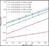 |
Fig. 1 Fits to the expanding cluster in simulations by least-squares. The dots are from different time nodes; i.e., t = 0 Myr, 1 Myr, 2 Myr, 3 Myr, and 4 Myr. Here, “k” is the slope of the linear fit with the unit pc/M⊙, and “r” represents the Pearson correlation coefficient. |
3 Cluster radii in observations
In observations, different methods are used to estimate the size of a cluster, and the measured radius can be the half-mass radius, rh, or the full radius, rf. We can trace the evolution of rh and rf at the same time in simulations, which can be the benchmarks to classify the observed radii of very young star clusters (<4 Myr).
3.1 Half-mass radius
For the clusters in Lada et al. (1991), they determined cluster boundaries using the magnitude limit of mK < 13, and also required the lowest contour level to correspond to a surface density of two times the background density. In Carpenter et al. (1993), the magnitude limit is mH = 15.5. For the samples in these two papers, the boundaries of the clusters based on the identification criteria are probably not representative of the total extent of the cluster, and therefore the measured radius is likely to be smaller than the full radius rf of the cluster. As shown in Fig. 2a, the samples can be well fitted by the 1 Myr expanding line. Considering that the ages of these clusters are indeed around 1 Myr (Weidner et al. 2013), the simulations well explain the observed radii, and the measured radii in these observations are close to the half-mass radii of the clusters.
For the embedded cluster catalog in Lada & Lada (2003), as shown in Fig. 2b, the samples move systematically upwards, indicating older ages or larger radius measurements. The catalog gives the absolute magnitude limits mK of the corresponding imaging observations. Figure 2c shows the distribution of the magnitude limits. If we take mK < 15.5 and mK > 15.5 as high and low standards of the magnitude limits, the median radii of the clusters in the two groups are ≈0.61 pc and 0.76 pc, respectively. As expected, low standards indeed give slightly larger radius estimates due to the larger star counts. According to the selection criterion in Lada & Lada (2003), most of the clusters should have an age of around 1 Myr. We note that part of the samples of Carpenter et al. (1993) and Lada et al. (1991) are also found in the catalog of Lada & Lada (2003). Except for those samples with significant deviations, the almost systematic upshifting of most of the sample in Lada & Lada (2003) in Fig. 2b may be attributed to the low standards, which cause slightly larger radius estimates. However, given that accurate age estimation of embedded clusters is always very challenging in observations, the differences are just as likely to be caused by the different ages of the cluster samples.
3.2 Full radius
In some observations, the cluster radius was measured by: 1. The surface density profile decreases until it reaches a constant value (Faustini et al. 2009); 2. The density profile exceeds twice the standard deviation of the surface density in the surrounding field (Carpenter 2000; Kumar et al. 2006). It seems these observations measured the full cluster radius. In Fig. 3, we used the rh − Mecl and rf − Mecl relations to compare with the observations. The two relations give the age estimates of ≈2 Myr and ≈1 Myr, respectively. For the samples in Kumar et al. (2006), they are the youngest stellar clusters associated with massive protostellar candidates, thus, their ages should be ≤1 Myr. Therefore, the rf – Mecl relation gives a better fit than the rh–Mecl relation, which means the above observations roughly measured the full radii of the samples. The ages of the clusters in Carpenter (2000) and Faustini et al. (2009) are <2 Myr and ≤1 Myr, respectively. All of them are well fitted in Fig. 3.
3.3 Recent observations
Readers may consider the observational sample presented above to be dated and therefore question its reliability. Below, we further validate the above results using more recent observations.
The MYStIX (Massive Young Star-Forming Complex Study in Infrared and X-ray) project (Feigelson et al. 2013) examined 20 nearby (d<3.6 kpc) massive star-forming regions (MSFRs) using a combination of archival Chandra X-ray imaging, 2MASS+UKIDSS near-infrared (NIR), and Spitzer mid-infrared (MIR) survey data. The catalog of 31 784 young stars from the project includes both high-mass and low-mass stars, and both disk-bearing and disk-free stars (Broos et al. 2013). Although the MYStIX samples are not “complete”, the identification of young stars was performed in a uniform way for the different regions, enabling a comparative analysis of the stellar populations within these diverse regions. Across 17 massive star-forming regions in the MYStIX project, Kuhn et al. (2014) identified 142 subclusters (their “subclusters” being synonymous to the embedded clusters here) of young stars using finite mixture models. Their physical parameters were listed in Kuhn et al. (2015), such as the radius, the age, and the total number of stars. Getman et al. (2014) provided age estimates for over 100 subclusters using the novel AgeJX method, which encompasses a wide age range between 0.5 and 5 Myr, showing that individual regions often present spatial segregation.
The radii of the subclusters in Table 1 of Kuhn et al. (2015) are four times the core radius based on their model and are considered by these authors to be roughly the projected halfmass radii. As shown in Fig. 4a, the rh–Mecl relations can well fit the observations. However, the ages assigned to individual young stars may exhibit considerable uncertainty due to statistical errors in luminosities, uncertainties in dereddening, and the inherent variability in the X-ray-luminosity–mass relation. Additionally, different evolutionary models might introduce systematic shifts in ages (Getman et al. 2014; Kuhn et al. 2015). To further complicate this discussion, the identification of subclusters in Kuhn et al. (2014) is not based on the Plummer profile as used in the present simulations. Furthermore, the table only provides the total number of stars in each subcluster, and to derive mass we assume an average stellar mass of 0.5 M⊙. This may lead to underestimation of the mass of the subcluster. Using the samples from Lada & Lada (2003), in Fig. A.1, the actual correlation between the total number of stars and the mass of an embedded cluster systematically shifts upward compared to the 0.5 M⊙ assumption. Despite many uncertainties, the good fittings in Fig. 4a remain impressive. Moreover, the expansion of subclusters has been confirmed in Kuhn et al. (2015) and Kuhn et al. (2019) from observations.
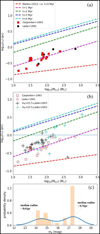 |
Fig. 2 Fitting the mass–radius relation of embedded clusters in observations using N-body simulations. (a) Dashed lines are the rh − Mecl relations at different time nodes (t = 1 Myr, 2 Myr, 3 Myr and 4 Myr), i.e. the 1 Myr, 2 Myr, 3 Myr and 4 Myr expanding lines. Red squares and black dots represent the clusters from Carpenter et al. (1993) and Lada et al. (1991), respectively. (b) Plus symbols show the clusters from Lada & Lada (2003), while the black and red plus symbols show the clusters selected by the magnitude limits mK<15.5 and mK>15.5, respectively. The horizontal line marks the position of the radius r = 1 pc. (c) Distribution of the magnitude limits mK of the clusters in Lada & Lada (2003). |
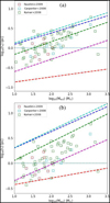 |
Fig. 3 Fitting the mass–radius relation of embedded clusters in observations using N-body simulations. Colored squares represent the clusters from Carpenter (2000), Kumar et al. (2006) and Faustini et al. (2009). The horizontal line marks the position of the radius r = 1 pc. The dashed lines are color-coded according to age as in Figs. 1 and 2. |
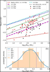 |
Fig. 4 Fitting the mass–radius relation of embedded clusters in observations using N-body simulations. (a) Dashed lines are the rh–Mecl relations at different time nodes. Red and black dots represent the subclusters from Kuhn et al. (2014), which have ages of >1.6 Myr and <1.6 Myr, respectively. The dashed black line represents the fitted massradius relation. Here, “k” is the slope of the linear fitting with units of pc/M⊙, and “r” is the Pearson correlation coefficient. (b) Age distribution of the subclusters in Table 1 of Kuhn et al. (2015). |
4 Mass–radius relation
Assuming all embedded clusters have the Plummer profile with the Plummer radius rpl , the mass within radius r is
![Mathematical equation: $M(r) = {M_{{\rm{ecl}}}}{{{{\left( {{r \over {{r_{{\rm{pl}}}}}}} \right)}^3}} \over {{{\left[ {1 + {{\left( {{r \over {{r_{{\rm{pl}}}}}}} \right)}^2}} \right]}^{{3 \over 2}}}}}.$](/articles/aa/full_html/2024/11/aa52064-24/aa52064-24-eq3.png) (3)
(3)
The full radius (0.9 mass fraction) and the half-mass radius (0.5 mass fraction) satisfy rf ≈ 3.707 rpl and rh ≈ 1.305rpl, and therefore rf ≈ 2.84rh (Kroupa 2008). For the samples discussed above, we can unify their radii to the half-mass radii. The radii of the samples in Lada et al. (1991), Carpenter et al. (1993) and Lada & Lada (2003) can be approximated to the half-mass radii. For the samples in Carpenter (2000), Kumar et al. (2006) and Faustini et al. (2009), their radii need to be divided by 2.84. As shown in Fig. 5, different samples can indeed merge together after the unification. We fitted the mass–radius relation for all samples, which gives a slope of ≈0.33 (dashed cyan line in Fig. 5). If we fit the samples in Lada et al. (1991); Carpenter et al. (1993); Lada & Lada (2003) and Carpenter (2000); Kumar et al. (2006); Faustini et al. (2009) separately, the slopes are ≈0.43 (dashed black line in Fig. 5) and ≈0.32 (dashed blue line in Fig. 5), respectively. Only using the samples in Kuhn et al. (2015) gives a slope of ≈0.36 in Fig. 4a.
The equation (4) of Pfalzner et al. (2016) has a steeper slope of ≈0.58 (dashed yellow line in Fig. 5). Pfalzner et al. (2016) also found that all collected data in the K-band show a mass–radius relation with a similar slope. These authors therefore argued that clusters might “grow” from low-mass clusters to their final mass without changing their size, and their size would be determined by the extent of the clump. However, as shown in this work, the unique mass–radius relation of Pfalzner et al. (2016) actually reflects the expansion of embedded clusters. There is no self-similar mass–radius development during the evolution of embedded clusters, because the expanding lines in Fig. 2 are not parallel at the beginning. The real initial mass–radius relation of embedded clusters (equation (1)) is significantly different from the relation of Pfalzner et al. (2016). Any observable cluster is already in a state of expansion to varying degrees. Thus, the current mass–radius relation of clusters cannot reveal their initial formation conditions. In Pfalzner et al. (2016), there is no cluster containing a thousand stars and with a half mass radius of <0.4 pc in their samples because all the samples are expanding and thus detach from the initial compact configuration predicted by the initial mass–radius relation of embedded clusters (equation (1)). As confirmed in the following section, even the embedded clusters in ATLASGAL clumps with HII regions (HII-clumps) are already in expansion.
In Pfalzner et al. (2016), all collected samples show a mass– radius relation with a similar slope, also shown in Figs. 2, 3, 4a and 5 in this work, although different methods were used to determine the radius and mass in different observations. As explained in Pfalzner et al. (2016), assuming a unique mass–radius relation and a self-similar mass–radius development throughout, the different mass and radius measurements simply move the data points along the line of the mass–radius relation. In the discussion above, we have excluded this interpretation. Another simple explanation is that all clusters initially have the Plummer profile and then expand through the expulsion of residual gas, as modeled in Sect. 2.1. As done above, different radii in different observations can be unified to the half-mass radii. This operation will not change the slope of the mass–radius relation, which only shifts the line of the mass–radius relation, as shown in Pfalzner et al. (2016) and this work, also see the discussion in Zhou et al. (2024c).
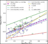 |
Fig. 5 Fitting the mass–radius relation of embedded clusters in observations using N-body simulations. For the samples in Fig. 3, their radii were divided by 2.84, and then merged with the samples in Fig. 2. The radii of all samples were unified to the half-mass radius. The yellow dashed line is the mass–radius relation of Pfalzner et al. (2016). Dashed cyan, black, and blue lines represent the mass–radius relations of all samples, the samples in Lada et al. (1991); Carpenter et al. (1993); Lada & Lada (2003) and the samples in Carpenter (2000); Kumar et al. (2006); Faustini et al. (2009), respectively. Here, “k” is the slope of the fitting with the unit pc/M⊙, and “r” represents the Pearson correlation coefficient. |
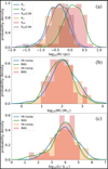 |
Fig. 6 Comparison of the radius, mass, and bolometric luminosity of embedded clusters in HII clumps of Urquhart et al. (2022) and the clusters (IRAS sources) in Kumar et al. (2006). |
5 Expansion of embedded clusters in HII-clumps
The sample in Kumar et al. (2006) consists of the youngest stellar clusters associated with massive protostellar candidates (IRAS sources). As such, they are comparable to embedded clusters in HII-clumps, as shown in Figs. 6 and 7. The cluster radius in Kumar et al. (2006) is the effective radius Reff, which is approximated to the full radius of the cluster, as described in Sect. 3.2. The radii of HII-clumps, Rcl, in Urquhart et al. (2022) are determined from the number of pixels within the FWHM contour, that is, those above 50 per cent of the peak of the ATLASGAL dust continuum emission. As shown in Fig. 6a, Reff is significantly larger than Rcl. However, Reff /2.84 is comparable with Rcl. Reff /2.84 is approximated to the half-mass radius of the cluster in Kumar et al. (2006), as discussed in Sect. 4. Therefore, Rcl measured in Urquhart et al. (2022) is close to the half-mass radius of the embedded cluster in a HII-clump. A HII-clump mass Mcl and its embedded star cluster mass Mecl satisfy Mecl = SFE * Mcl, where SFE is the final star formation efficiency of the clump. As discussed in Sect. 2.1, we take SFE = 0.33. In Fig. 7, the masses and radii of the embedded clusters in HII-clumps can be well fitted on the rh–Mecl plane. Generally, the samples are between the 0 and 1 Myr expanding lines, which is consistent with their ages (≤1 Myr). However, some samples are located under the initial 0 Myr line. This may be due to the fact that these clumps reach a higher gas density during gas collapse than implied by the rh − Mecl relation for embedded clusters, or it could be that the measurement of their radii is biased or affected by resolution. As shown in Urquhart et al. (2022), evolutionary sequences still exist within HII-clumps. For the samples under the initial 0 Myr line, they may be so young that the inner cluster formation is not yet complete.
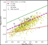 |
Fig. 7 Fitting the masses and sizes of embedded clusters in HII clumps (yellow dots) using the expanding lines in Figs. 1 and 2. Blue circles represent the clusters in Kumar et al. (2006). |
6 Conclusion
We used standard N-body simulations as in previous works. The comparison between the previously deduced initial conditions of the simulations with the data used here has not been performed up to date, and this work constitutes a first step in an attempt to understand the data in terms of a realistic physical model that was developed previously on different data of young clusters and stellar populations.
In this work, we traced the evolution of the rh–Mecl and rf– Mecl relations in the first 4 Myr using direct N-body simulations. We used the expanding lines at different time nodes as benchmarks to classify the observed radii of very young star clusters. The good fit of the expanding lines to the samples compellingly suggests that the observed very young clusters are in expansion. After unifying the radii of all samples to the half-mass radii, we fitted the mass–radius relations for different categories, finding that they are comparable with the mass–radius relation documented by Pfalzner et al. (2016). Thus, the mass–radius relation of Pfalzner et al. (2016) actually reflects the expansion of embedded clusters starting with the initial mass–radius relation of Marks & Kroupa (2012). We also suggest that even the embedded clusters in ATLASGAL clumps with HII regions (HII-clumps) are already in expansion. The collected samples all show a mass–radius relation with a similar slope, which may indicate that embedded clusters are born with a profile resembling that of the Plummer phase-space density distribution function (e.g., Aarseth et al. 1974; Heggie & Hut 2003). This is interesting, because the Plummer phase space density distribution function is the simplest analytical (two-parameter) distribution function that solves the time-independent collisionless Boltzmann equation (e.g., Kroupa 2008), and because the molecular cloud filaments in which stars have been found to have Plummer-like cross sections (André et al. 2022), as well as both open (Röser et al. 2011; Röser & Schilbach 2019) and globular star clusters (Plummer 1911) are also well described by Plummer models.
Appendix A Comparison of simulations under different parameter settings
In the simulations, all clusters are fully mass segregated (S =1) and no fractalization. We also assumed a star formation efficiency (SFE) of 0.33. However, some young clusters are observed to be highly substructured and do now show evidence of mass segregation. Moreover, the SFE also has a certain range of variation. Therefore, it is necessary to explore how varying these parameters might affect the cluster evolution and the masssize relation. We compared fully mass segregated (S =1) and partly mass segregated (S =0.5) in Fig. A.3, with and without fractalization in Fig. A.2, and found the results are similar. Moreover, 100% and 44% initial binary fractions also give similar results, as shown in Fig. A.4. SFE=0.33 and SFE=0.2 in Fig. A.5 give different results, because a smaller SFE implies a larger gas volume, which affects the gas expulsion process. However, given the measurement error of cluster age, simulations using SFE = 0.2 can still roughly explain the observations.
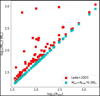 |
Fig. A.1 Correlation between the total number of stars and the mass of embedded cluster. |
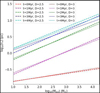 |
Fig. A.2 Comparison of the expanding lines for clusters with and without fractalization. The settings for other parameters are the same as described in Sec. 2.1. We arranged a fractal distribution of stars within a sphere of constant average density, following a similar method as outlined in Goodwin & Whitworth (2004). The likelihood of a sub-box receiving a star can be represented by 2D–3, where D represents the fractal dimension. When D is set to 3.0, there is no fractality observed since the probability becomes one. More details can be found in Küpper et al. (2011) and the user manual for the McLuster code. |
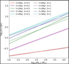 |
Fig. A.3 Comparison of the expanding lines for clusters with fully mass-segregated (S =1) and partially mass-segregated (S =0.5) configurations. The settings for other parameters are the same as described in Sec. 2.1. |
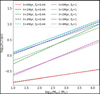 |
Fig. A.4 Comparison of the expanding lines for clusters with 100% ( fb =1) and 44% ( fb=0.44) initial binary fractions. The settings for other parameters are the same as described in Sec. 2.1. |
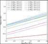 |
Fig. A.5 Comparison of the expanding lines for clusters with SFE=0.33 and SFE=0.2. The settings for other parameters are the same as described in Sec. 2.1. |
References
- Aarseth, S. J., Henon, M., & Wielen, R. 1974, A&A, 37, 183 [NASA ADS] [Google Scholar]
- Adams, F. C., Proszkow, E. M., Fatuzzo, M., & Myers, P. C. 2006, ApJ, 641, 504 [NASA ADS] [CrossRef] [Google Scholar]
- Alfaro, E. J., & Román-Zúñiga, C. G. 2018, MNRAS, 478, L110 [Google Scholar]
- André, P. J., Palmeirim, P., & Arzoumanian, D. 2022, A&A, 667, L1 [CrossRef] [EDP Sciences] [Google Scholar]
- Banerjee, S., & Kroupa, P. 2013, ApJ, 764, 29 [CrossRef] [Google Scholar]
- Banerjee, S., & Kroupa, P. 2014, ApJ, 787, 158 [NASA ADS] [CrossRef] [Google Scholar]
- Banerjee, S., & Kroupa, P. 2015, MNRAS, 447, 728 [NASA ADS] [CrossRef] [Google Scholar]
- Banerjee, S., & Kroupa, P. 2017, A&A, 597, A28 [NASA ADS] [CrossRef] [EDP Sciences] [Google Scholar]
- Banerjee, S., & Kroupa, P. 2018, in Astrophysics and Space Science Library, 424, The Birth of Star Clusters, ed. S. Stahler, 143 [NASA ADS] [CrossRef] [Google Scholar]
- Banerjee, S., Kroupa, P., & Oh, S. 2012, ApJ, 746, 15 [Google Scholar]
- Banerjee, S., Belczynski, K., Fryer, C. L., et al. 2020, A&A, 639, A41 [NASA ADS] [CrossRef] [EDP Sciences] [Google Scholar]
- Bastian, N., & Goodwin, S. P. 2006, MNRAS, 369, L9 [NASA ADS] [CrossRef] [Google Scholar]
- Bate, M. R., Tricco, T. S., & Price, D. J. 2014, MNRAS, 437, 77 [NASA ADS] [CrossRef] [Google Scholar]
- Baumgardt, H., & Kroupa, P. 2007, MNRAS, 380, 1589 [NASA ADS] [CrossRef] [Google Scholar]
- Belloni, D., Askar, A., Giersz, M., Kroupa, P., & Rocha-Pinto, H. J. 2017, MNRAS, 471, 2812 [NASA ADS] [CrossRef] [Google Scholar]
- Brandner, W. 2008, in Astronomical Society of the Pacific Conference Series, 387, Massive Star Formation: Observations Confront Theory, eds. H. Beuther, H. Linz, & T. Henning, 369 [NASA ADS] [Google Scholar]
- Brinkmann, N., Banerjee, S., Motwani, B., & Kroupa, P. 2017, A&A, 600, A49 [NASA ADS] [CrossRef] [EDP Sciences] [Google Scholar]
- Broos, P. S., Getman, K. V., Povich, M. S., et al. 2013, ApJS, 209, 32 [NASA ADS] [CrossRef] [Google Scholar]
- Cantat-Gaudin, T., Jordi, C., Wright, N. J., et al. 2019, A&A, 626, A17 [NASA ADS] [CrossRef] [EDP Sciences] [Google Scholar]
- Carpenter, J. M. 2000, AJ, 120, 3139 [Google Scholar]
- Carpenter, J. M., Snell, R. L., Schloerb, F. P., & Skrutskie, M. F. 1993, ApJ, 407, 657 [NASA ADS] [CrossRef] [Google Scholar]
- Chen, L., de Grijs, R., & Zhao, J. L. 2007, AJ, 134, 1368 [NASA ADS] [CrossRef] [Google Scholar]
- Das, S. R., Gupta, S., Prakash, P., Samal, M., & Jose, J. 2023, ApJ, 948, 7 [NASA ADS] [CrossRef] [Google Scholar]
- Della Croce, A., Dalessandro, E., Livernois, A. R., & Vesperini, E. 2024, A&A, 683, A10 [NASA ADS] [CrossRef] [EDP Sciences] [Google Scholar]
- Dib, S., Gutkin, J., Brandner, W., & Basu, S. 2013, MNRAS, 436, 3727 [NASA ADS] [CrossRef] [Google Scholar]
- Dinnbier, F., Kroupa, P., & Anderson, R. I. 2022, A&A, 660, A61 [NASA ADS] [CrossRef] [EDP Sciences] [Google Scholar]
- Duarte-Cabral, A., Bontemps, S., Motte, F., et al. 2013, A&A, 558, A125 [NASA ADS] [CrossRef] [EDP Sciences] [Google Scholar]
- Faustini, F., Molinari, S., Testi, L., & Brand, J. 2009, A&A, 503, 801 [NASA ADS] [CrossRef] [EDP Sciences] [Google Scholar]
- Feigelson, E. D., Townsley, L. K., Broos, P. S., et al. 2013, ApJS, 209, 26 [Google Scholar]
- Flaccomio, E., Micela, G., Peres, G., et al. 2023, A&A, 670, A37 [NASA ADS] [CrossRef] [EDP Sciences] [Google Scholar]
- Getman, K. V., Feigelson, E. D., Kuhn, M. A., et al. 2014, ApJ, 787, 108 [Google Scholar]
- Giacobbo, N., Mapelli, M., & Spera, M. 2018, MNRAS, 474, 2959 [Google Scholar]
- Goodwin, S. P., & Bastian, N. 2006, MNRAS, 373, 752 [Google Scholar]
- Goodwin, S. P., & Whitworth, A. P. 2004, A&A, 413, 929 [NASA ADS] [CrossRef] [EDP Sciences] [Google Scholar]
- Gutermuth, R. A., Megeath, S. T., Myers, P. C., et al. 2009, ApJS, 184, 18 [Google Scholar]
- Heggie, D., & Hut, P. 2003, The Gravitational Million-Body Problem: A Multidisciplinary Approach to Star Cluster Dynamics (Cambridge University Press) [Google Scholar]
- Hurley, J. R., Pols, O. R., & Tout, C. A. 2000, MNRAS, 315, 543 [Google Scholar]
- Hurley, J. R., Tout, C. A., & Pols, O. R. 2002, MNRAS, 329, 897 [Google Scholar]
- Jadhav, V. V., Kroupa, P., Wu, W., Pflamm-Altenburg, J., & Thies, I. 2024, A&A, 687, A89 [NASA ADS] [CrossRef] [EDP Sciences] [Google Scholar]
- Kirk, H., & Myers, P. C. 2011, ApJ, 727, 64 [Google Scholar]
- Kroupa, P. 1995a, MNRAS, 277, 1491 [Google Scholar]
- Kroupa, P. 1995b, MNRAS, 277, 1507 [NASA ADS] [Google Scholar]
- Kroupa, P. 2001, MNRAS, 322, 231 [NASA ADS] [CrossRef] [Google Scholar]
- Kroupa, P. 2005, in ESA Special Publication, Vol. 576, The Three-Dimensional Universe with Gaia, eds. C. Turon, K. S. O’Flaherty, & M. A. C. Perryman, 629 [NASA ADS] [Google Scholar]
- Kroupa, P. 2008, in The Cambridge N-Body Lectures, 760, ed. S. J. Aarseth, C. A. Tout, & R. A. Mardling, 181 [NASA ADS] [CrossRef] [Google Scholar]
- Kroupa, P., Petr, M. G., & McCaughrean, M. J. 1999, New A, 4, 495 [NASA ADS] [CrossRef] [Google Scholar]
- Kroupa, P., Aarseth, S., & Hurley, J. 2001, MNRAS, 321, 699 [NASA ADS] [CrossRef] [Google Scholar]
- Kuhn, M. A., Feigelson, E. D., Getman, K. V., et al. 2014, ApJ, 787, 107 [Google Scholar]
- Kuhn, M. A., Feigelson, E. D., Getman, K. V., et al. 2015, ApJ, 812, 131 [NASA ADS] [CrossRef] [Google Scholar]
- Kuhn, M. A., Hillenbrand, L. A., Sills, A., Feigelson, E. D., & Getman, K. V. 2019, ApJ, 870, 32 [CrossRef] [Google Scholar]
- Kuhn, M. A., Hillenbrand, L. A., Carpenter, J. M., & Avelar Menendez, A. R. 2020, ApJ, 899, 128 [NASA ADS] [CrossRef] [Google Scholar]
- Kumar, M. S. N., Keto, E., & Clerkin, E. 2006, A&A, 449, 1033 [NASA ADS] [CrossRef] [EDP Sciences] [Google Scholar]
- Kumar, M. S. N., Palmeirim, P., Arzoumanian, D., & Inutsuka, S. I. 2020, A&A, 642, A87 [EDP Sciences] [Google Scholar]
- Küpper, A. H. W., Maschberger, T., Kroupa, P., & Baumgardt, H. 2011, MNRAS, 417, 2300 [Google Scholar]
- Lada, C. J., & Lada, E. A. 2003, ARA&A, 41, 57 [Google Scholar]
- Lada, E. A., Depoy, D. L., Evans, Neal J.I., & Gatley, I. 1991, ApJ, 371, 171 [NASA ADS] [CrossRef] [Google Scholar]
- Lane, J., Kirk, H., Johnstone, D., et al. 2016, ApJ, 833, 44 [Google Scholar]
- Lim, B., Hong, J., Yun, H.-S., et al. 2020, ApJ, 899, 121 [CrossRef] [Google Scholar]
- Lim, B., Nazé, Y., Hong, J., et al. 2022, AJ, 163, 266 [NASA ADS] [CrossRef] [Google Scholar]
- Littlefair, S. P., Naylor, T., Jeffries, R. D., Devey, C. R., & Vine, S. 2003, MNRAS, 345, 1205 [NASA ADS] [CrossRef] [Google Scholar]
- Longmore, S. N., Kruijssen, J. M. D., Bastian, N., et al. 2014, in Protostars and Planets VI, eds. H. Beuther, R. S. Klessen, C. P. Dullemond, & T. Henning, 291 [Google Scholar]
- Machida, M. N., & Matsumoto, T. 2012, MNRAS, 421, 588 [NASA ADS] [Google Scholar]
- Marks, M., & Kroupa, P. 2012, A&A, 543, A8 [NASA ADS] [CrossRef] [EDP Sciences] [Google Scholar]
- Marks, M., Kroupa, P., & Oh, S. 2011, MNRAS, 417, 1684 [NASA ADS] [CrossRef] [Google Scholar]
- Megeath, S. T., Gutermuth, R., Muzerolle, J., et al. 2016, AJ, 151, 5 [Google Scholar]
- Motte, F., Bontemps, S., & Louvet, F. 2018, ARA&A, 56, 41 [NASA ADS] [CrossRef] [Google Scholar]
- Mužić, K., Almendros-Abad, V., Bouy, H., et al. 2022, A&A, 668, A19 [NASA ADS] [CrossRef] [EDP Sciences] [Google Scholar]
- Myers, P. C. 2009, ApJ, 700, 1609 [Google Scholar]
- Nony, T., Robitaille, J. F., Motte, F., et al. 2021, A&A, 645, A94 [NASA ADS] [CrossRef] [EDP Sciences] [Google Scholar]
- Oh, S., & Kroupa, P. 2016, A&A, 590, A107 [NASA ADS] [CrossRef] [EDP Sciences] [Google Scholar]
- Oh, S., & Kroupa, P. 2018, MNRAS, 481, 153 [NASA ADS] [CrossRef] [Google Scholar]
- Oh, S., Kroupa, P., & Pflamm-Altenburg, J. 2015, ApJ, 805, 92 [Google Scholar]
- Pang, X., Li, Y., Yu, Z., et al. 2021, ApJ, 912, 162 [NASA ADS] [CrossRef] [Google Scholar]
- Pavlik, V., Kroupa, P., & Šubr, L. 2019, A&A, 626, A79 [NASA ADS] [CrossRef] [EDP Sciences] [Google Scholar]
- Peretto, N., Fuller, G. A., Duarte-Cabral, A., et al. 2013, A&A, 555, A112 [NASA ADS] [CrossRef] [EDP Sciences] [Google Scholar]
- Pfalzner, S., Kirk, H., Sills, A., et al. 2016, A&A, 586, A68 [NASA ADS] [CrossRef] [EDP Sciences] [Google Scholar]
- Plummer, H. C. 1911, MNRAS, 71, 460 [Google Scholar]
- Plunkett, A. L., Fernández-López, M., Arce, H. G., et al. 2018, A&A, 615, A9 [NASA ADS] [CrossRef] [EDP Sciences] [Google Scholar]
- Portegies Zwart, S. F., McMillan, S. L. W., & Gieles, M. 2010, ARA&A, 48, 431 [NASA ADS] [CrossRef] [Google Scholar]
- Proszkow, E.-M., & Adams, F. C. 2009, ApJS, 185, 486 [NASA ADS] [CrossRef] [Google Scholar]
- Proszkow, E.-M., Adams, F. C., Hartmann, L. W., & Tobin, J. J. 2009, ApJ, 697, 1020 [NASA ADS] [CrossRef] [Google Scholar]
- Röser, S., & Schilbach, E. 2019, A&A, 627, A4 [NASA ADS] [CrossRef] [EDP Sciences] [Google Scholar]
- Röser, S., Schilbach, E., Piskunov, A. E., Kharchenko, N. V., & Scholz, R. D. 2011, A&A, 531, A92 [NASA ADS] [CrossRef] [EDP Sciences] [Google Scholar]
- Schneider, N., Csengeri, T., Hennemann, M., et al. 2012, A&A, 540, L11 [NASA ADS] [CrossRef] [EDP Sciences] [Google Scholar]
- Smith, N., Stassun, K. G., & Bally, J. 2005, AJ, 129, 888 [NASA ADS] [CrossRef] [Google Scholar]
- Stutz, A. M., & Gould, A. 2016, A&A, 590, A2 [NASA ADS] [CrossRef] [EDP Sciences] [Google Scholar]
- Swiggum, C., D’Onghia, E., Alves, J., et al. 2021, ApJ, 917, 21 [NASA ADS] [CrossRef] [Google Scholar]
- Tanikawa, A., Yoshida, T., Kinugawa, T., Takahashi, K., & Umeda, H. 2020, MNRAS, 495, 4170 [NASA ADS] [CrossRef] [Google Scholar]
- Tobin, J. J., Offner, S. S. R., Kratter, K. M., et al. 2022, ApJ, 925, 39 [NASA ADS] [CrossRef] [Google Scholar]
- Urquhart, J. S., Wells, M. R. A., Pillai, T., et al. 2022, MNRAS, 510, 3389 [NASA ADS] [CrossRef] [Google Scholar]
- Vázquez-Semadeni, E., Palau, A., Ballesteros-Paredes, J., Gómez, G. C., & Zamora-Avilés, M. 2019, MNRAS, 490, 3061 [Google Scholar]
- von Steiger, R., & Zurbuchen, T. H. 2016, ApJ, 816, 13 [Google Scholar]
- Wang, L., Kroupa, P., & Jerabkova, T. 2019, MNRAS, 484, 1843 [NASA ADS] [CrossRef] [Google Scholar]
- Wang, L., Iwasawa, M., Nitadori, K., & Makino, J. 2020a, MNRAS, 497, 536 [NASA ADS] [CrossRef] [Google Scholar]
- Wang, L., Kroupa, P., Takahashi, K., & Jerabkova, T. 2020b, MNRAS, 491, 440 [Google Scholar]
- Weidner, C., Kroupa, P., & Pflamm-Altenburg, J. 2013, MNRAS, 434, 84 [NASA ADS] [CrossRef] [Google Scholar]
- Whitmore, B. C., Zhang, Q., Leitherer, C., et al. 1999, AJ, 118, 1551 [CrossRef] [Google Scholar]
- Wright, N. J., Jeffries, R. D., Jackson, R. J., et al. 2019, MNRAS, 486, 2477 [CrossRef] [Google Scholar]
- Wright, N. J., Jeffries, R. D., Jackson, R. J., et al. 2023, arXiv e-prints [arXiv: 2311.08358] [Google Scholar]
- Wuchterl, G., & Tscharnuter, W. M. 2003, A&A, 398, 1081 [NASA ADS] [CrossRef] [EDP Sciences] [Google Scholar]
- Xu, F., Wang, K., Liu, T., et al. 2024, ApJS, 270, 9 [NASA ADS] [CrossRef] [Google Scholar]
- Yan, Z., Jerabkova, T., & Kroupa, P. 2023, A&A, 670, A151 [NASA ADS] [CrossRef] [EDP Sciences] [Google Scholar]
- Yang, W. J., Menten, K. M., Yang, A. Y., et al. 2022, A&A, 658, A192 [NASA ADS] [CrossRef] [EDP Sciences] [Google Scholar]
- Zhang, Q., Fall, S. M., & Whitmore, B. C. 2001, ApJ, 561, 727 [NASA ADS] [CrossRef] [Google Scholar]
- Zhang, Y., Tanaka, K. E. I., Tan, J. C., et al. 2022, ApJ, 936, 68 [NASA ADS] [CrossRef] [Google Scholar]
- Zhou, J.-W., Liu, T., Evans, N. J., et al. 2022, MNRAS, 514, 6038 [NASA ADS] [CrossRef] [Google Scholar]
- Zhou, J. W., Dib, S., & Kroupa, P. 2024a, PASP, 136, 094302 [NASA ADS] [CrossRef] [Google Scholar]
- Zhou, J. W., Kroupa, P., & Dib, S. 2024b, PASP, 136, 094301 [NASA ADS] [CrossRef] [Google Scholar]
- Zhou, J.-w., Kroupa, P., & Dib, S. 2024c, A&A, 688, L19 [NASA ADS] [CrossRef] [EDP Sciences] [Google Scholar]
All Tables
All Figures
|
Fig. 1 Fits to the expanding cluster in simulations by least-squares. The dots are from different time nodes; i.e., t = 0 Myr, 1 Myr, 2 Myr, 3 Myr, and 4 Myr. Here, “k” is the slope of the linear fit with the unit pc/M⊙, and “r” represents the Pearson correlation coefficient. |
| In the text | |
|
Fig. 2 Fitting the mass–radius relation of embedded clusters in observations using N-body simulations. (a) Dashed lines are the rh − Mecl relations at different time nodes (t = 1 Myr, 2 Myr, 3 Myr and 4 Myr), i.e. the 1 Myr, 2 Myr, 3 Myr and 4 Myr expanding lines. Red squares and black dots represent the clusters from Carpenter et al. (1993) and Lada et al. (1991), respectively. (b) Plus symbols show the clusters from Lada & Lada (2003), while the black and red plus symbols show the clusters selected by the magnitude limits mK<15.5 and mK>15.5, respectively. The horizontal line marks the position of the radius r = 1 pc. (c) Distribution of the magnitude limits mK of the clusters in Lada & Lada (2003). |
| In the text | |
|
Fig. 3 Fitting the mass–radius relation of embedded clusters in observations using N-body simulations. Colored squares represent the clusters from Carpenter (2000), Kumar et al. (2006) and Faustini et al. (2009). The horizontal line marks the position of the radius r = 1 pc. The dashed lines are color-coded according to age as in Figs. 1 and 2. |
| In the text | |
|
Fig. 4 Fitting the mass–radius relation of embedded clusters in observations using N-body simulations. (a) Dashed lines are the rh–Mecl relations at different time nodes. Red and black dots represent the subclusters from Kuhn et al. (2014), which have ages of >1.6 Myr and <1.6 Myr, respectively. The dashed black line represents the fitted massradius relation. Here, “k” is the slope of the linear fitting with units of pc/M⊙, and “r” is the Pearson correlation coefficient. (b) Age distribution of the subclusters in Table 1 of Kuhn et al. (2015). |
| In the text | |
|
Fig. 5 Fitting the mass–radius relation of embedded clusters in observations using N-body simulations. For the samples in Fig. 3, their radii were divided by 2.84, and then merged with the samples in Fig. 2. The radii of all samples were unified to the half-mass radius. The yellow dashed line is the mass–radius relation of Pfalzner et al. (2016). Dashed cyan, black, and blue lines represent the mass–radius relations of all samples, the samples in Lada et al. (1991); Carpenter et al. (1993); Lada & Lada (2003) and the samples in Carpenter (2000); Kumar et al. (2006); Faustini et al. (2009), respectively. Here, “k” is the slope of the fitting with the unit pc/M⊙, and “r” represents the Pearson correlation coefficient. |
| In the text | |
|
Fig. 6 Comparison of the radius, mass, and bolometric luminosity of embedded clusters in HII clumps of Urquhart et al. (2022) and the clusters (IRAS sources) in Kumar et al. (2006). |
| In the text | |
|
Fig. 7 Fitting the masses and sizes of embedded clusters in HII clumps (yellow dots) using the expanding lines in Figs. 1 and 2. Blue circles represent the clusters in Kumar et al. (2006). |
| In the text | |
|
Fig. A.1 Correlation between the total number of stars and the mass of embedded cluster. |
| In the text | |
|
Fig. A.2 Comparison of the expanding lines for clusters with and without fractalization. The settings for other parameters are the same as described in Sec. 2.1. We arranged a fractal distribution of stars within a sphere of constant average density, following a similar method as outlined in Goodwin & Whitworth (2004). The likelihood of a sub-box receiving a star can be represented by 2D–3, where D represents the fractal dimension. When D is set to 3.0, there is no fractality observed since the probability becomes one. More details can be found in Küpper et al. (2011) and the user manual for the McLuster code. |
| In the text | |
|
Fig. A.3 Comparison of the expanding lines for clusters with fully mass-segregated (S =1) and partially mass-segregated (S =0.5) configurations. The settings for other parameters are the same as described in Sec. 2.1. |
| In the text | |
|
Fig. A.4 Comparison of the expanding lines for clusters with 100% ( fb =1) and 44% ( fb=0.44) initial binary fractions. The settings for other parameters are the same as described in Sec. 2.1. |
| In the text | |
|
Fig. A.5 Comparison of the expanding lines for clusters with SFE=0.33 and SFE=0.2. The settings for other parameters are the same as described in Sec. 2.1. |
| In the text | |
Current usage metrics show cumulative count of Article Views (full-text article views including HTML views, PDF and ePub downloads, according to the available data) and Abstracts Views on Vision4Press platform.
Data correspond to usage on the plateform after 2015. The current usage metrics is available 48-96 hours after online publication and is updated daily on week days.
Initial download of the metrics may take a while.