| Issue |
A&A
Volume 691, November 2024
|
|
|---|---|---|
| Article Number | A283 | |
| Number of page(s) | 13 | |
| Section | Planets and planetary systems | |
| DOI | https://doi.org/10.1051/0004-6361/202451750 | |
| Published online | 20 November 2024 | |
High-resolution transmission spectroscopy of the hot-Saturn HD 149026b
1
DiSAT, Università degli Studi dell’Insubria,
via Valleggio 11,
22100
Como,
Italy
2
INAF – Osservatorio Astronomico di Brera,
via E. Bianchi 46,
23807
Merate (LC),
Italy
3
INFN, Sezione Milano-Bicocca,
P.za della Scienza 3,
20126
Milano,
Italy
★ Corresponding author; fbiassoni@studenti.uninsubria.it
Received:
1
August
2024
Accepted:
11
October
2024
Advances in modern technology have enabled the characterization of exoplanetary atmospheres, which can be achieved by exploitation of the transmission spectroscopy technique. We performed visible (VIS) and near-infrared (NIR) high-resolution spectroscopic observations of one transit of HD 149026b, a close-in orbit sub-Saturn exoplanet by using the GIARPS configuration at the Telescopio Nazionale Galileo (TNG). We first analyzed the radial-velocity data, refining the value of the projected spin-orbit obliquity (λ). We then performed transmission spectroscopy, looking for absorption signals from the planetary atmosphere. We find no evidence for Hα, Na I D2-D1, Mg I, or Li I in the VIS and metastable helium triplet He I(23S) in the NIR using a line-by-line approach. The non-detection of HeI is also supported by theoretical simulations. With the use of the cross-correlation technique (CCF), we do not detect Ti I, V I, Cr I, Fe I, or VO in the visible, or indeed CH4, CO2, H2O, HCN, NH3, or VO in the NIR. Our non-detection of Ti I in the planetary atmosphere is in contrast with a previous detection. We performed injection-retrieval tests, finding that our dataset is sensitive to our Ti I model. The non-detection supports the Ti I cold-trap theory, which is valid for planets with Teq < 2200 K, such as HD 149026b. Although we do not attribute it directly to the planet, we find a possibly significant Ti I signal that is highly redshifted (≃+20 km s−1 ) with respect to the planetary rest frame. Redshifted signals are also found in the Fe I and Cr I maps. While we can exclude an eccentric orbit as the cause of this redshifted Ti I signal, we investigated the possibility of material accretion falling onto the star – which is possibly supported by the presence of strong Li I in the stellar spectrum - but obtained inconclusive results. The analysis of multiple transits datasets could shed more light on this target.
Key words: techniques: spectroscopic / planets and satellites: atmospheres / planets and satellites: detection / planets and satellites: gaseous planets / stars: chemically peculiar / planetary systems
© The Authors 2024
 Open Access article, published by EDP Sciences, under the terms of the Creative Commons Attribution License (https://creativecommons.org/licenses/by/4.0), which permits unrestricted use, distribution, and reproduction in any medium, provided the original work is properly cited.
This article is published in open access under the Subscribe to Open model. Subscribe to A&A to support open access publication.
1 Introduction
With advancements in instruments and facilities, the focus of the scientific community has shifted from the discovery of exoplanets to their characterization, with one of the main goals the understanding of their atmospheric compositions. Presently, transmission spectroscopy is the most efficient technique for characterizing the properties of the atmospheres of exoplanets (e.g., Birkby 2018; Madhusudhan 2019). During transits, exoplanetary atmospheres absorb specific wavelengths of the radiation emitted by their host stars, providing insights into their elemental composition in the stellar light coming to us. High-resolution spectroscopy (resolving power R ≳ 20 000) enables us to glean a wealth of information about exoplanet parameters and atmospheric content. This technique allows us to identify atoms and molecules by isolating their distinct, high cross-section absorption lines, which are unique to each species. As an example, we are able to identify the Na I doublet (e.g., Wyttenbach et al. 2015), the Ca II H & K lines (e.g., Yan et al. 2019), Hα (e.g., Jensen et al. 2012), and the metastable He I triplet (e.g., Allart et al. 2018). Alternatively, the use of the cross-correlation function (CCF; e.g., Snellen et al. 2010; Brogi et al. 2012; Hoeijmakers et al. 2018; Borsa et al. 2022; Prinoth et al. 2023) offers another powerful method for detecting species for which strong lines cannot be identified. These types of analysis are mainly employed for the characterization of the atmospheres of the so-called hot Jupiters (Bell & Cowan 2018), that is, gas giants in a close-in orbit. Due to their proximity to the host star, these planets experience intense extreme-ultraviolet (XUV; 10–912 Å) and far-ultraviolet (FUV; 912–2585 Å) irradiation, leading to the heating and possibly inflation of their atmospheres (e.g., Owen 2019; Biassoni et al. 2024).
Among the class of gas giants, a particularly interesting case is that of HD 149026b. The planet was first detected using the radial-velocity (RV) method by Sato et al. (2005), who measured a radius and mass (in Jupiter units) of Rp = 0.725 ± 0.05 RJ and Mp = 0.36 ± 0.02 MJ, respectively. HD 149026b is more massive but smaller in size than Saturn, despite receiving intense irradiation from its parent star, which should lead to an inflated atmosphere (Sato et al. 2005). The planet’s high density, as evidenced by findings such as  cm−3 (Wolf et al. 2007),
  cm−3 (Torres et al. 2008), and ρp = 2.1 ± 0.8 g cm−3 (Southworth 2010), suggests a core that is rich in metals, as proposed by Sato et al. (2005), who estimated a core mass ≈67 M⊕, where M⊕ is the Earth’s mass. Subsequent studies echoed these high core estimations. Fortney et al. (2006) claimed a significant presence of heavy elements in both the core and envelope, estimating values of ≈60–93 M⊕; Burrows et al. (2007) inferred a core mass ranging between 80 and 110 M⊕; and Baraffe et al. (2008) and Carter et al. (2009) estimated heavy element core masses of ≈60–80 M⊕ and ≈45–70 M⊕, respectively.
A high core mass and high stellar metallicity ([Fe/H] = 0.36 ± 0.05; Sato et al. 2005) appear to be crucial prerequisites for a planet with a large atmospheric metallicity (Zhang et al. 2018). Several atmospheric models have been proposed to unravel the composition of HD 149026b. Fortney et al. (2006) observed a hot stratosphere, and attributed this to the absorption of stellar flux by TiO and VO, while Stevenson et al. (2012), analyzing Spitzer secondary eclipse observations, adopted a chemical equilibrium model and suggested the presence of large amounts of CO and CO2, with moderate heat redistribution, high metallicity, and the absence of thermal inversion on the dayside. Zhang et al. (2018) analyzed Spitzer phase-curve observations at 3.6 and 4.5 µm and inferred a high albedo, possibly explained by the presence of reflective cloud layers in the planet’s upper atmosphere. Recently analyses based on transmission spectroscopy conducted with the High Dispersion Spectrograph (Noguchi et al. 2002) on the Subaru telescope were performed by Ishizuka et al. (2021). These authors reported a tentative ≃4.4σ detection of Ti I, and a marginal ≃2.8σ detection of Fe I, alongside non-detections of Sc I, V I, Cr I, Mn I, Co I, and TiO. The presence of Ti I without TiO suggests a super-solar C/O ratio (Ishizuka et al. 2021). Recently, Bean et al. (2023) analyzed the HD 149026b dayside emission obtained with the James Webb Space Telescope (JWST). Similarly to prior studies, these authors concluded that the planet exhibits a highly super-solar metallicity ![$\left( {[M/H] = 2.09_{ - 0.32}^{ + 0.35}} \right)$](/articles/aa/full_html/2024/11/aa51750-24/aa51750-24-eq3.png) and a high carbon-to-oxygen ratio ([C/O] = 0.84 ± 0.03), which further support the detection of CO2 and H2O in HD 149026b. The same dataset was analyzed by Gagnebin et al. (2024) using a 1D radiative-convective-thermochemical equilibrium model from which new values of planet atmospheric metallicity are estimated to be ≃ 1.15 if VO is not included in the models, and ≃1.30 if it is. These values are approximately ten times smaller than those found by Bean et al. (2023).
and a high carbon-to-oxygen ratio ([C/O] = 0.84 ± 0.03), which further support the detection of CO2 and H2O in HD 149026b. The same dataset was analyzed by Gagnebin et al. (2024) using a 1D radiative-convective-thermochemical equilibrium model from which new values of planet atmospheric metallicity are estimated to be ≃ 1.15 if VO is not included in the models, and ≃1.30 if it is. These values are approximately ten times smaller than those found by Bean et al. (2023).
Spinelli et al. (2023) updated the HD 149026b parameters by exploiting more precise Gaia Data Release 2 (DR2; Gaia Collaboration 2018) distances, inferring a mass and radius of Mp = 0.28 ± 0.03 MJ and Rp = 0.74 ± 0.02 RJ, respectively. These values yield a planetary density of pp = 0.86 ± 0.09 g cm−3, consistent with the lowest estimates of previous works, such as,  cm−3 as in Bonomo et al. (2017), and
  cm−3 as in Carter et al. (2009). Given the results of Spinelli et al. (2023), we decided to shed more light on the atmospheric content of HD 149026b with high-resolution transmission spectroscopy. To this aim, we collected data from two transits at the Telescopio Nazionale Galileo (TNG) equipped with high-resolution visible and near-infrared (NIR) spectrographs, namely the High Accuracy Radial velocity Planet Searcher North (HARPS-N; R ≃ 115 000) and GIANO-B (R ≃ 50 000), respectively.
In this work, we describe our observations, data analysis, and scientific results. The paper is organized as follows: Details regarding the observations can be found in Sect. 2, while Sects. 3 and 4 cover our modeling of the Rossiter-McLaughlin effect, center-to-limb variations, and data analyses. A discussion of the results of our data analysis and concluding remarks are provided in Sect. 6.
Observations performed with the two instruments.
2 Observations
We observed one transit of HD 149026b on June 14 2022 with the HARPS-N and GIANO-B high-resolution spectrographs mounted at the TNG (Program A45TAC_30, PI Borsa). We exploited the GIARPS configuration (Claudi et al. 2016), which allows us to observe simultaneously with the two spectrographs. A second scheduled transit on 3 April 2022 was lost due to bad weather. The wavelength range of the acquired spectra span from the visible (VIS; 3900–6900 Å, HARPS-N) to near-infrared (NIR; 9400–24200 Å, GIANO-B). With GIANO-B, we collected 78 spectra with exposures of 200 sec per nodding position (ABAB pattern). Meanwhile, with HARPS-N, we observed a total of 64 spectra with an exposure time of 300 sec. All the spectra were reduced with the standard DRS pipelines v3.7 and v1.6.1 for HARPS-N (Cosentino et al. 2012) and GIANO-B (Rainer et al. (2018); Harutyunyan et al. (2018)), respectively. A summary of the observations is shown in Table 1.
During the observations, we lost about half an hour at the transit ingress because of a problem with the instrument guiding system. A strong loss of flux was also experienced during the transit, which was solved by performing a repointing procedure. Figure 1 shows the signal-to-noise ratio (S/N) obtained with HARPS-N and GIANO-B at 5500 and 16 300 Å, respectively. For our analysis, we discarded all the spectra with low S/N with respect to the adjacent ones (see Fig. 1), ultimately performing our analysis on a total of 61 (75) HARPS-N (GIANO-B) spectra.
3 Rossiter-McLaughlin effect
During a transit, the partial occultation of the stellar disk by the planet induces a distortion in the observed stellar spectrum, leading to apparent variations of the derived stellar RVs. This specific phenomenon is commonly referred to as the Rossiter-McLaughlin (RML) effect (Rossiter 1924; McLaughlin 1924). The amplitude and shape of the RML effect are mainly dependent on the projected stellar rotation velocity (v sin i), the projected spin-orbit inclination (λ), the impact parameter (b), and the Rp/R★ ratio, where R★ is the stellar radius. An analysis of the RML effect enables the extraction of these planetary and stellar parameters, which are later used in the transmission spectroscopy (Sect. 4.3). In order to model the RML effect, we employed the CaRM code, a semi-automated tool (Cristo et al. 2022) that employs a Markov chain Monte Carlo algorithm. Details of our analysis of the RML effect are presented in Appendix A. Globally, the values we obtain for projected rotational speed, systemic velocity (γ), RV amplitude, and inclination (i) are in agreement with literature results. In particular, we refine the projected spin-orbit angle λ = 2.5 ± 5.3 deg, in agreement with the literature value (λ = 12 ± 7 deg; Albrecht et al. 2012) but with smaller error bars (Fig. 2). The RVs and their best fit are shown in Fig. 2.
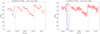 |
Fig. 1 HARPS-N and GIANO-B S/N for the second night evaluated at 5500 and 16 300 Å, respectively. The red dots represent the S/N of the spectra used for transmission spectroscopy analysis, while the blue ones are discarded. The two vertical orange lines denote the T1 and T4 transit contact points. |
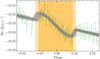 |
Fig. 2 Result from the RML fitting procedure performed with CaRM. The red line is the best-fit model, and the gray shadows are a random sample of the posterior distribution. The yellow regions show the ingress and egress of the transit, while the orange region shows where the planet is fully transiting the stellar disk. |
4 Transmission spectroscopy
The main goal of our observations is to look for the atmosphere of HD 149026b using high-resolution transmission spectroscopy. We started our analysis from the merged 1D spectra (s1d) provided by the HARPS-N DRS. Similarly, we analyzed the 71st GIANO-B spectral order, searching for the presence of the metastable helium triplet He I(23S) at ≃10 830 Å. We chose to work with the echelle spectral orders (msld) in the NIR band instead of the merged s1d spectra to improve the normalization of the GIANO-B spectra.
4.1 Telluric correction and wavelength calibration
We performed correction for telluric H2O and O2 lines on all HARPS-N spectra using Molecfit v. 4.3.1 (Smette et al. 2015; Kausch et al. 2015), following the guidelines specified in Allart et al. (2017), but slightly modifying the wavelength ranges of the correction. The left panel of Fig. 3 provides an example of the telluric correction obtained using Molecfit, near the Hα line.
We also used Molecfit v. 4.3.1 to correct the GIANO-B spectra, but following a different recipe. The GIANO-B wavelength calibration may be slightly inconsistent between the different echelle orders due to the characteristics of the U-Ne calibration lamp (the number of useful emission lines varies greatly between the orders). While Molecfit accounts for some wavelength shift in the observed spectrum, trying to correct the whole merged GIANO-B spectra resulted in p-Cygni-like residuals due to the slight misalignment of the echelle orders. For this reason, we worked with the ms 1d GIANO-B spectra, where the echelle orders are still separated, and we ran Molecfit on each order independently. Another complication arose from the fact that the NIR wavelength range is heavily affected by the telluric absorption – due to the combination of the wide wavelength range of GIANO-B and the large telluric contribution, the computational time needed to model and remove the telluric lines from all the 50 orders of a single GIANO-B spectrum is quite high. In order to speed up the process, we computed the model only once every ten spectra, assuming that the atmospheric conditions did not vary significantly in this time. To account for any possible variation due to the position of the star on the slit (positions A and B of the nodding observational strategy), we worked separately on the A and B spectra, computing one model for every ten A spectra and one for every ten B spectra. While we globally removed H2O, O2, CO2, N2O, CH4, and CO from the whole spectrum, working on the separate orders allowed us to model only the atmospheric molecules present in each echelle order. The right panel of Fig. 3 provides an example of telluric correction near the He I(23S) lines.
Interval used for the transmission spectroscopy analysis.
4.2 Transmission spectrum extraction
We extracted the transmission spectrum following the guidelines outlined in Wyttenbach et al. (2015), performing the procedure in a short wavelength interval bracketing each of the atmospheric lines investigated (see Table 2). As a first step, all the spectra were normalized and shifted to the stellar reference frame. We then generated an average reference stellar spectrum (Master-Out, Mout) by calculating a weighted mean of all the out-of-transit spectra. We then divided each spectrum by Mout and derived the residual spectra Ri accordingly. These Ri were further normalized to eliminate any trend possibly imprinted by imperfect continuum atmospheric dispersion corrections. In order to maximize any potential planetary signal (if present), all Ri were shifted into the planet reference frame, considering a circular orbit with parameters from Table 3. We then computed a weighted mean of all the in-transit residual spectra to obtain the final average transmission spectrum. These transmitted spectra have a shortened wavelength range with respect to the initial intervals chosen for each element analyzed; this is due to the Doppler shifts and subsequent interpolation procedures adopted during the transmission spectroscopy analysis, which lead to divergence at the edges of the wavelength ranges (Table 2). After each interpolation the wavelength bin width was maintained constant at the value of 0.01 Å.
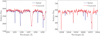 |
Fig. 3 Example of Molecf it telluric correction. The left panel refers to the HARPS-N telluric correction in proximity to the Hα line, while the right panel shows the GIANO-B telluric correction in proximity to He I(23S). Both spectra are taken from the first exposure. |
Physical parameters for the HD 149026 system.
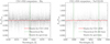 |
Fig. 4 CLV+RM models (red) compared with transmission spectra (light gray) around the Hα and Na I D doublet wavelength regions. Green lines show the position of the theoretical values of Hα, Na I D2, and D1 lines. The CLV+RML model contamination is well within the data noise. |
4.3 Analysis of single lines
We extracted the transmission spectrum in the wavelength ranges of the Mg I triplet (5167.32–5172.68–5183.60 Å), Na I D2-D1 (5889.95–5895.92 Å), Hα (6562.81 Å), Li I (6707.76 Å) in the optical band, and the He I(23S) triplet (10 829.09–10830.25–10 830.34 Å) in the infrared band1.
During a transit, one must consider that the host star is not a homogeneously bright disk; rather its surface brightness changes with the distance from disk center, a phenomenon known as center-to-limb variation (CLV). Moreover, the star rotates. These stellar properties affect the emitted spectrum occulted during transit through CLV and the RML effect, respectively, which in turn can affect the transmission spectrum in various ways, such as by modifying the shape of the line profiles and/or by causing false atmospheric detections (e.g., Yan et al. 2017; Borsa & Zannoni 2018; Casasayas-Barris et al. 2020). Given the characteristics of our target, namely its low projected rotational velocity and small Rp/R★ ratio, we expect minimal-to-low contamination from RML and CLV. In order to verify if this is indeed the case, we modeled CLV and RML as outlined in Yan et al. (2017) on a few lines (Hα, the Na I doublet, and the Mg I triplet) using the same methodology as that employed by Borsa et al. (2021). The star was modeled as a disk, and mapped on a fine grid with 0.01 resolution. At each point of the grid, we calculated the angle between the normal to the stellar surface and the line of sight, µ = cos θ, and the projected rotational velocity (rescaling the υ sin i and using rigid body rotation). A spectrum was then assigned to each point of the grid by a quadratic interpolation on µ, and Doppler-shifting according to the stellar rotation the model spectra created using the tool Spectroscopy Made Easy (SME; Piskunov & Valenti 2017), with the line list from the VALD database (Ryabchikova et al. 2015) and the ATLAS9 (Kurucz 1993; Castelli & Kurucz 2003) stellar atmospheric models. The model spectra were created with null rotational velocity for 21 different µ values at the resolving power of HARPS-N. Using the orbital information from Table 3, we then simulated the transit of the planet, calculating the stellar spectrum for different orbital phases as the average spectrum of the non-occulted modeled sections. In the last step, we divided each spectrum for a master stellar spectrum calculated out of transit, obtaining information on the relevance of CLV+RML effects at each in-transit orbital phase. We then moved everything in the planetary rest frame, calculating the simulated CLV+RML effects on the transmission spectrum.
Figure 4 shows a comparison between the transmission spectra of Hα and the Na I D doublet and the simulated CLV+RML contamination. The latter is well within the noise of the data, confirming expectations. As CLV+RML are negligible in the transmission spectrum, we ignore them in our subsequent analyses.
We performed a Gaussian fit around all the lines of interest using a linear regression method (see the footnote in Appendix A). In the visible band, our analysis led to a non-detection of all the considered lines, namely Hα, Na I D2-D1, the Mg I triplet, and Li I. Examples of the results are shown in Fig. 5. We estimated the upper limits of these lines by calculating the standard deviation within ±0.5 Å from their reference wavelengths (see Table 4).
Indeed, the depth of the stellar lines strongly affects our ability to put strong limits on the atmospheric heights. We used Mout to measure the stellar flux intensity within the core of all these lines relative to the continuum. As shown in Table 4, most of the transmission signals we were looking for are affected by a relatively low stellar flux. As a result, the S/N of the transmission spectrum of the planet is constrained by these low values of the flux, potentially meaning that any possible planetary signal is lost in the noise.
We also surveyed the NIR band in search of the metastable helium triplet He I(23S) at ≃10 830 Å. This state of helium predominantly appears in planets orbiting K-type stars (Oklopčić 2019), and its abundance and relative absorption signal depend upon various factor, such as the hardness ratio (LXUV/LFUV) of the stellar spectrum, the planetary orbital distance, the planetary Hill radius, and the He-to-H abundance ratio in the planet’s outer atmosphere (e.g., Biassoni et al. 2024).
We applied the same technique used for the visible band to extract the transmission spectrum close to the He I(23S) lines. The result shows substantial noise and a sinusoidal pattern (Fig. 6), which is a known artefact in GIANO-B transmission spectra (e.g., Guilluy et al. 2023). In order to improve the normalization, we fitted a sinusoidal function of the form A ⋅ sin(x) + B ⋅ cos(bx) + mx + C, for which we divided the transmission spectrum (gray curve in Fig. 6). During the analysis, we took into account the two telluric OH doublets (10 829.46–10 829.15 Å and 10 831.38–10 831.29 Å, wavelengths in air; Oliva et al. 2013), whose emission can notably affect this wavelength region (e.g., Guilluy et al. 2023). We shifted them in the stellar reference system after correcting for the systemic velocity and the barycentric velocity of the Earth. In this reference system,, these lines fall at 10 829.84–10 829.54 Å and 10 831.77–10 831.67 Å, respectively. To remove them, we completely masked the regions between [10 832.38–10 832.89] Å and [10834.53–10834.81] Å.
Similarly to the analysis in the visible band, the helium profile was fitted with two Gaussian profiles, as in the Na I doublet.
The doublet lines at 10 830.25–10 830.34 Å were considered blended (Kirk et al. 2022). The prior on the center of the doublet, µ = 10 830.29 Å, was set between ±0.2 Å to prevent significant deviation from the fit due to the high noise level in the spectrum. The fit suggests an absorption pattern near the He I(23S) doublet (Figure 7), but the profile lacks clear definition, and its deviation from the continuum is only at ≃2.3 σ.
The absence of a significant He I(23S) signal in the planetary atmosphere was further investigated theoretically. Using the 1D photoionization hydrodynamic code ATES (Caldiroli et al. 2021) and the Transmission Probability Module (TPM; Biassoni et al. 2024), we modelled the outflow of HD 149026b, estimating its mass-loss rate alongside the number density of He I(23S) and the transmission spectrum. To achieve this simulation, we employed the HD 149026 spectrum provided by Behr et al. (2023) rescaled at the planetary orbital distance assuming a circular orbit. In the simulation, we used planetary and stellar parameters from Table 3. To match our observations, we convolved the simulated absorption profile with the GIANO-B instrumental resolution (R = 50 000, assumed as Gaussian), while also considering the planet’s rotation under the assumptions of tidal locking and a radius equal to  , where h represents the theoretical absorption depth at the He I(23S) doublet core derived from TPM, and δ = (Rp /R⋆)2 denotes the transit depth. The simulation produces a mass-loss rate of ≈5 × 10¹⁰ g s−1, resulting in an absorption depth of He I(23S) of ≃0.7% (blue curve in Fig. 7), of the same order as the error bars in the data.
HD 149026b transmission spectroscopy upper limits.
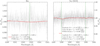 |
Fig. 5 Hα and Na I D2-D1 transmission spectra. The gray points are our transmission spectra, the red line the best Gaussian fit, and the black dots are the result of resampling the transmission spectra with a bin size of 0.3 A. |
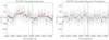 |
Fig. 6 He I(23S) transmission spectrum. Left panel: in gray Fin/Fout obtained with the transmission spectroscopy analysis. A sinusoidal shape is evident. The red line is the sinusoidal fit obtained using the relation described in the text. Right panel: gray transmission spectrum divided by the sinusoidal red fit. Black dots represent the binned spectra with equally spaced bins of 0.3 Å, while vertical dashed green lines show the positions of the theoretical He I(23 S) lines in vacuum. |
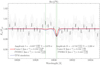 |
Fig. 7 He I(23 S) normalized transmission spectrum in comparison with the double Gaussian fit and TPM simulation. |
4.4 Cross-correlation analysis
Line-by-line transmission spectroscopy is very effective in detecting absorption lines with large cross-sections in exo- planetary atmospheres. However, it often fails in detecting the numerous intrinsically faint lines expected from atoms such as Fe, Ti, and V, and from molecules. To increase the S/N, the CCF is indeed a more powerful tool (e.g., Snellen et al. 2010; Brogi et al. 2012; Hoeijmakers et al. 2019; Borsa et al. 2021).
In our analysis, we employed the CCF technique to investigate the presence of Ti I, V I, Cr I, Fe I, and VO in the visible band, and CH4 , CO2, H2O, HCN, NH3 , and VO in the NIR. For this purpose, we constructed the templates employing petitRADTRANS (Mollière et al. 2019), a python package that allows calculation of the planetary transmission and emission spectra. We constructed models using the parameters of Table 3, with an isothermal atmospheric profile with T = 2000 K, a metallicity [Fe/H] = 0.36 (Ishizuka et al. 2021), and a continuum pressure of 10 mbar, which is consistent with the white-light transit depth. The models, which, as expected, generated variation in planetary radius with wavelength, were then translated in (Rp /R⋆)2 and convolved with the HARPS-N resolving power. We normalized the templates and convolved them as well in order to match the planet’s rotational velocity, assuming tidal locking.
For our CCF analysis, we began by performing similar steps to those of the line-by-line analysis on the s1d spectra, but using the e2ds spectra instead (e.g., Stangret et al. 2020). This allows us to perform a better normalization when working on the whole spectral range of the spectrograph. We employed Molecfit to correct the 1D s1d HARPS-N spectra and applied the retrieved telluric profile to correct the e2ds spectral orders (e.g., Hoeijmakers et al. 2020). To enhance the quality of the CCF analysis, we excluded the first five orders and the last one from all exposures due to their low S/N, focusing on the wavelength range 4000–6840 Å. The e2ds spectral orders were then reformatted into matrices, with each one containing all the exposures of the same order (Fig. 8, top panel). As we are working with ground-based instruments, we must account for the flux variation over time. Therefore, we normalized each exposure by dividing it by the mean value across the pixels (Fig. 8, lower panel).
We then started our CCF calculation:
 (1)
(1)
where υ is the velocity at which the template is shifted and k refers to the pixels in our 1D spectrum x, which contains all the stacked normalized and telluric-corrected spectral orders, while T represents the template. The CCF is done in the range −200 km s−1 < v < 200 km s−1 , in steps of 1 km s−1 . The resulting CCF was shifted to the stellar reference frame, interpolated within the RV range −150 km s−1 < v < 150 km s−1 in steps of 1 km s−1 , and normalized by the CCF Mout . For a more accurate normalization, we further divided this CCF by the median values across the exposures. To eliminate low-frequency fluctuations and to smooth the CCF, we conducted a fast Fourier transform, cutting any velocity beyond 100 km s−1 for each exposure. The resulting final CCFs for the inspected elements are given in Figs. 9 and 10. The blurred region at phase ≃ − 0.02 is caused by a lack of data; we discarded them due to their low S/N.
To detect any possible planetary atmospheric signal, we generated the Kp−Vsys maps by shifting all the CCFs in different planetary reference systems. We considered circular orbits with various Kp velocities in the range 0–300 km s−1, with a step of 1 km s−1, and averaged all the in-transit residual CCFs. Kp−Vsys maps were then divided by the standard deviation of the overall map, after excluding a region of ±100 km s−1for both RV and Kp values centered at the expected Kp value (156.19 km s−1) and 0 km s−1 RV. This normalization yields Kp−Vsys maps in terms of S/N as shown in Figs. 9 and 10. The blurred regions in the CCFs at the beginning of the transit are due to the lack of data for these orbital phases (see Fig. 1 and Sect. 2).
From the analysis of our data, we do not find evidence (signal with S/N > 4) for the presence of any of the species searched for in the atmosphere of the planet in proximity to the expected planetary signal. The non-detection of TiI, in particular, is in contrast with the previous detection of this element by Ishizuka et al. (2021). To verify that our data precision and analysis approach is sensitive to the expected signals, we injected our planetary atmospheric models into the data prior to any analysis using a planetary orbital velocity opposite to the theoretical one (e.g., Pelletier et al. 2021). The e2ds spectra were then analyzed following the prescription described at the beginning of Sect. 4.4. CCF and Kp−Vsys maps containing the injected models are shown in Fig. 9. In this way, we retrieved the injected signals of Ti I and Fe I at the expected Kp and RV value at ~ 4.1 σ (Kp = −174 km s−1, RV = 0 km s−1) and ~ 3.3 σ (Kp = −152 km s−1, RV = −1 km s−1), respectively. For V I and Cr I, the data lack the necessary precision to detect these species with our planetary model, meaning we cannot obtain a clear detection.
As the results of CCF analysis may strongly depend on the line lists used to create the templates (e.g., Gandhi et al. 2020), we verified our Ti I non-detection by creating templates with different line lists. We used the line lists from Kurucz (Kurucz 1993), VALD (Piskunov et al. 1995), and NIST downloaded from the DACE2 database and converted them into petitRADTRANS format to create new models. We also downloaded the isothermal templates at 2000 K, 2500 K, and 3000 K from Kitzmann et al. (2023). We then re-performed the CCFs using all these templates, obtaining very similar results and TiI non-detections each time.
We also performed CCFs in the IR channel on the ms1d GIANO-B spectral orders, searching for the presence of molecules such as CH4, CO2, H2O, HCN, NH3 , and VO. In this channel we also performed telluric correction using Molecfit, with a dedicated procedure as described in Sect. 4. Many orders are not usable due to their low S/N and the intrinsic transmissivity of the Earth’s atmosphere. Therefore, we masked the flux of the following GIANO-B diffraction orders before the CCF analysis for each exposure: 81, 80, 79, 69, 68, 67, 66, 57, 56, 55, 54, 53, 52, 51, 43, 42, 41, 40, 39, 38, 37, and 32. Figure 11 shows an example of two different orders where the Molecfit telluric correction was applied successfully and where it failed, respectively.
The CCF and Kp−Vsys maps for the selected models where then retrieved with the same normalization procedure employed in the VIS band with the HARPS-N e2ds spectral orders. Our analysis did not show any detection of an exoplanetary absorption signal in the NIR band either (Fig. 12).
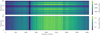 |
Fig. 8 Flux variation for all the exposures for the 59th HARPS-N spectral order (6538.7–6612.3 Å). The strong absorption line at pixel ≃1200 is the stellar Hα line. The top panel (before the normalization) shows the 59th spectral order along all the exposures. The bottom panel shows the result after the normalization. |
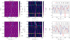 |
Fig. 9 CCF (left) and Kp–Vsys (center) maps for Ti I and Fe I. The horizontal white lines in CCF maps correspond to the T1 and T4 contact points, while the cyan dash dotted and gold dotted lines mark the expected planetary Kp and -Kp of the injected signals, respectively. The white slanted line corresponds to the Doppler shadow curve. Cyan and gold arrows in Kp–Vsys maps point toward Kp and -Kp , respectively. Orange dash dotted and white dotted pointers point toward the minimum value of the maps between RV [−40, +40] km s−1, Kp [100,200] km s−1and that between RV [−40, +40] km s−1, Kp [−200, −100] km s−1, respectively. The red and navy lines in the last column are the 1D projection of the Kp– Vsys maps evaluated at the minima found around the theoretical and injected Kp . |
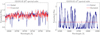 |
Fig. 11 Comparison between two different GIANO-B ms1d spectral orders, before (navy) and after (red) Molecfit correction. The left panel refers to the 34th spectral order, where the correction is successful. The right panel refers to the 41st spectral order, where correction does not work properly as telluric lines are saturated in this wavelength region. We did not consider the 41st spectral order and similar ones in our analyses and discarded them. |
5 Lithium in the stellar spectrum
When investigating planetary atmospheric signals, we also explored the lithium line at 6707.76 Å (Sect. 4.3). While we did not find this line in the planetary atmosphere, we noticed that it is clearly present in the master-out stellar spectrum (Fig. 13), which is not often the case for stars of this age because of its rapid depletion (e.g., Herbig 1965). Different age estimates for this system in the literature are in the range 1.9–2.6 Gyr, all of which are based on evolutionary tracks (Sato et al. 2005; Torres et al. 2008; Carter et al. 2009; Bonomo et al. 2017; Ment et al. 2018), with just one single exception (1.2 Gyr; Southworth 2010). However there is also the possibility of Li enrichment by, for example, the engulfment or accretion of a close-orbiting substel- lar companion (e.g., Soares-Furtado et al. 2021). Interestingly, Li et al. (2008) already suggested that the observed high metal- licity of HD 149026 may be confined to its surface layer as a consequence of pollution by the accretion of a gas giant or of a population of smaller-mass rocky planets.
As lithium is often a good age estimator (e.g., Herbig 1965; Jeffries et al. 2023), we investigated the possibility that its presence in the stellar spectrum could be at odds with the estimated age of the parent star. We estimated the equivalent width of the lithium 6707.76 Å line to be 36 ± 2 mÅ after de-blending it from the close Fe I line (e.g., Jeffries et al. 2023). We then inserted this value, together with the stellar temperature of Table 3, into the publicly available EAGLES code (Jeffries et al. 2023), which can give an independent stellar age estimate based on these two values. However, the results are totally unconstrained, likely because HD 149026 is too hot to use lithium as an indicator of stellar age. One other option to test the engulfment hypothesis would be to look at the 6Li/7Li isotopic ratio (e.g., Biazzo et al. 2022; Cuntz et al. 2000), but unfortunately our master-out stellar spectrum does not have sufficient S/N.
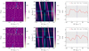 |
Fig. 12 CCF results for HCN and CO2 as in Fig. 9. At the end of the transit (phases ≃ 0.02), the noise in the CCF maps is due to the S/N drops for these exposures (see Fig. 1). |
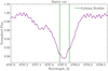 |
Fig. 13 Master-out stellar spectrum in proximity to the lithium doublet at 6707.76 Å. |
6 Discussion and conclusion
In this work, we analyzed VIS and NIR high-resolution spectroscopy observations of one transit of the exoplanet HD 149026b. After analyzing the Rossiter-McLaughlin effect, which allowed us to refine the projected spin-orbit angle of the planet, we performed transmission spectroscopy. We searched for atomic and molecular species in the atmosphere of the planet using both line-by-line and CCF techniques. We were not able to detect any of the searched species, finding only upper limits (Table 4). Indeed, the low flux in the core of the stellar lines, as is common for G-type stars, does not help the detection of small atmospheric signals.
It is worth noting that the Kp−Vsys maps for Ti I, Fe I, and to a lesser extent Cr I, may suggest a statistically significant (S/N=4.7, 4.2 and 3.3 respectively) signal at ≃ + (10–27) km s−1 relative to the expected position in RV, which is consistent with the planetary Kp value (Fig. 9 and 10). In the literature, there has been some debate regarding a possible eccentricity of the HD 149026b orbit, which could indeed lead to such a velocity shift for a signal from the planetary atmosphere. Wang & Ford (2011) found an eccentricity of e ≃ 0.19 ± 0.07. Harrington et al. (2007) detected an earlier occurrence of the secondary eclipse using Spitzer Space Telescope data approximately 3 minutes prior to the expected timing. Similarly, analyzing data obtained three years later, Knutson et al. (2009) predicted a secondary eclipse occurring approximately 21 minutes earlier than expected, possibly suggesting an eccentric orbit (e cos ω ≃ −0.0079, where ω is the argument of pericenter). However, the most recent analyses of both RVs and light curves of HD 149026b seem to be consistent with no eccentricity (Bonomo et al. 2017; Bean et al. 2023). To further decipher whether or not even a small eccentricity could cause this shift in any atmospheric signal, we verified whether not the values of e and ω parameters from Ment et al. (2018), when varying them within the error bars, could be the source of a shift this large. By calculating the RV curves with these parameters, we find curves that have a maximum RV of +6 km s−1 at mid-transit (phase = 0). When varying the parameters of e and ω within 3 σ, the most extreme curve shows an RV of +15.5 km s−1at phase = 0, which is still different from the observed signal at +20 km s−1. We are therefore inclined to exclude orbital eccentricity as a possible cause of these signals. An possible alternative, fascinating origin for this highly redshifted (≃ + 20 km s−1 ) signal is from material falling onto the star. Li et al. (2008) already suggested that this star may be highly metallic as a consequence of pollution by the accretion of planets. We investigated this hypothesis by studying the stellar lithium, but obtained inconclusive results. As we have only one transit observation and cannot confirm it independently, we prefer to attribute this signal to a spurious fluctuation. We however suggest that this should be further investigated with multiple high-resolution transit observations.
Ishizuka et al. (2021) reported a ≃4.4 σ detection of Ti I, together with a tentative ≃3 σ detection of FeI. These authors assumed a circular orbit. Contrary to Ishizuka et al. (2021), our analysis did not lead to the detection of either Ti I or Fe I in the data in the planetary rest frame. By performing injectionretrieval tests, we showed that our dataset is sensitive to the model of Ti I injected (S/N=4.1), and partially to the Fe I one (S/N=3.3). Our analysis of the HARPS-N dataset thus excludes the presence of Ti I in the atmosphere of the planet, in contrast with Ishizuka et al. (2021).
The absence of Ti I in the planetary atmosphere could be in line with the possible presence of a so-called “titanium cold trap.” A cold trap occurs when the equilibrium temperature is below the threshold for observing titanium in the upper atmosphere, as in the case of HD 149026b. According to Hoeijmakers et al. (2024), in planets with temperatures below ≃2200 K, Ti I condenses on the night side. This condensation could result in its absence throughout the planetary atmosphere, rendering it undetectable in the upper atmospheric layers where transmission spectroscopy is most effective as a probe. The cold-trap process can cause titanium to remain trapped on the planet’s night side due to inefficient advection. Alternatively, if titanium is circulated back into the day side, it may reside in high-pressure, low-altitude layers where it is barely detectable. In conclusion, the low equilibrium temperature and absence of Ti I in the planet’s atmosphere support the hypothesis of a titanium cold trap. Alternatively, the planet could possess a very dense atmosphere with extensive cloud coverage, making the atmosphere altogether optically thick at optical and near-infrared wavelengths.
Acknowledgements
We thank K. Biazzo and V. D’Orazi for useful suggestions on the presence of lithium in the stellar spectrum. FB acknowledges support from Bando Ricerca Fondamentale INAF 2023. This work has made use of the VALD database, operated at Uppsala University, the Institute of Astronomy RAS in Moscow, and the University of Vienna. We thank G. Fedrigo and M. Pozzarelli for advice on choosing colors for color-blind in CCF and Kp–Vsys figures. This work is based on observations collected with the Telescopio Nazionale Galileo (TNG).
Appendix A Rossiter-McLaughlin effect fitting
Set of priors used for the RM analysis.
The RVs were extracted by the HARPS-N DRS using a G2 mask with a CCF width of 20 km s−1. We used only the RVs extracted from spectra with S/N > 40 (identified as red dots in Fig. 1). CaRM employs a Markov chain Monte Carlo algorithm through emcee, a python module developed by Foreman-Mackey et al. (2013). Table A.1 provides all the priors used in our analysis. The guess parameter for the systemic RV used, γ = −18.035 km s−1, was taken from an approximate RVs data estimation. The other guess parameters we used are: the ratio between the semi-major axis and the stellar radius a/R⋆ = 5.98 (Spinelli et al. (2023)), the width of non-rotating star based on the HARPS-N resolving power (R ≃ 115 000) β0 = 2.6 km s−1, the width of the best Gaussian fit to the stellar CCFs σ0 = 4.37 km s−1 determined from a mean out-of-transit (master-out) CCF3, the macro-turbulence amplitude ζt = 4.53 km s−1 calculated from the Doyle et al. (2014) calibration valid for our stellar parameters, and the logarithmic jitter amplitude log σw = −11.5.
Within CaRM, we specifically employed the model ARoME, that requires a set of limb-darkening coefficients. CaRM provides them using LDTk (Parviainen & Aigrain 2015), a python package that automates and models the stellar limb-darkening profiles and coefficients employing spectra from the PHOENIX database (Husser et al. 2013). In our analysis a quadratic law was employed, yielding the following coefficients: ldc1 = 0.593, ldc2 = 0.123. Following Cristo et al. (2022), we used CaRM with 50 chains, 1,500 steps of burn-in and 3,000 for the production. The RVs and their best fit are shown in Fig. 2. The fit matches well the data, except for the initial values which show a trend that is likely caused by the telescope guiding issue detailed in Sect. 2. The results obtained from our analysis are reported in Table 3, with the posterior distributions shown in Fig. A.1.
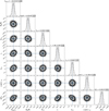 |
Fig. A.1 Posterior distributions of the radial velocity analysis obtained with CaRM. |
References
- Albrecht, S., Winn, J. N., Johnson, J. A., et al. 2012, ApJ, 757, 18 [NASA ADS] [CrossRef] [Google Scholar]
- Allart, R., Lovis, C., Pino, L., et al. 2017, A&A, 606, A144 [NASA ADS] [CrossRef] [EDP Sciences] [Google Scholar]
- Allart, R., Bourrier, V., Lovis, C., et al. 2018, Science, 362, 1384 [Google Scholar]
- Baraffe, I., Chabrier, G., & Barman, T. 2008, A&A, 482, 315 [NASA ADS] [CrossRef] [EDP Sciences] [Google Scholar]
- Bean, J. L., Xue, Q., August, P. C., et al. 2023, Nature, 618, 43 [NASA ADS] [CrossRef] [Google Scholar]
- Behr, P. R., France, K., Brown, A., et al. 2023, AJ, 166, 35 [NASA ADS] [CrossRef] [Google Scholar]
- Bell, T. J., & Cowan, N. B. 2018, ApJ, 857, L20 [Google Scholar]
- Biassoni, F., Caldiroli, A., Gallo, E., et al. 2024, A&A, 682, A115 [NASA ADS] [CrossRef] [EDP Sciences] [Google Scholar]
- Biazzo, K., D’Orazi, V., Desidera, S., et al. 2022, A&A, 664, A161 [NASA ADS] [CrossRef] [EDP Sciences] [Google Scholar]
- Birkby, J. L. 2018, arXiv e-prints [arXiv:1806.04617] [Google Scholar]
- Bonomo, A. S., Desidera, S., Benatti, S., et al. 2017, A&A, 602, A107 [NASA ADS] [CrossRef] [EDP Sciences] [Google Scholar]
- Borsa, F., & Zannoni, A. 2018, A&A, 617, A134 [NASA ADS] [CrossRef] [EDP Sciences] [Google Scholar]
- Borsa, F., Allart, R., Casasayas-Barris, N., et al. 2021, A&A, 645, A24 [EDP Sciences] [Google Scholar]
- Borsa, F., Giacobbe, P., Bonomo, A. S., et al. 2022, A&A, 663, A141 [NASA ADS] [CrossRef] [EDP Sciences] [Google Scholar]
- Brogi, M., Snellen, I. A. G., de Kok, R. J., et al. 2012, Nature, 486, 502 [Google Scholar]
- Burrows, A., Hubeny, I., Budaj, J., & Hubbard, W. B. 2007, ApJ, 661, 502 [NASA ADS] [CrossRef] [Google Scholar]
- Caldiroli, A., Haardt, F., Gallo, E., et al. 2021, A&A, 655, A30 [NASA ADS] [CrossRef] [EDP Sciences] [Google Scholar]
- Carter, J. A., Winn, J. N., Gilliland, R., & Holman, M. J. 2009, ApJ, 696, 241 [NASA ADS] [CrossRef] [Google Scholar]
- Casasayas-Barris, N., Pallé, E., Yan, F., et al. 2020, A&A, 635, A206 [NASA ADS] [CrossRef] [EDP Sciences] [Google Scholar]
- Castelli, F., & Kurucz, R. L. 2003, in Modelling of Stellar Atmospheres, 210, eds. N. Piskunov, W. W. Weiss, & D. F. Gray, A20 [NASA ADS] [Google Scholar]
- Claudi, R., Benatti, S., Carleo, I., et al. 2016, SPIE Conf. Ser., 9908, 99081A [NASA ADS] [Google Scholar]
- Cosentino, R., Lovis, C., Pepe, F., et al. 2012, SPIE Conf. Ser., 8446, 84461V [Google Scholar]
- Cristo, E., Santos, N. C., Demangeon, O., et al. 2022, A&A, 660, A52 [NASA ADS] [CrossRef] [EDP Sciences] [Google Scholar]
- Cuntz, M., Saar, S. H., & Musielak, Z. E. 2000, ApJ, 533, L151 [Google Scholar]
- Del Pozzo, W., & Veitch, J. 2022, CPNest: Parallel nested sampling, Astrophysics Source Code Library [record ascl:2205.021] [Google Scholar]
- Doyle, A. P., Davies, G. R., Smalley, B., Chaplin, W. J., & Elsworth, Y. 2014, MNRAS, 444, 3592 [Google Scholar]
- Foreman-Mackey, D., Hogg, D. W., Lang, D., & Goodman, J. 2013, PASP, 125, 306 [Google Scholar]
- Fortney, J. J., Saumon, D., Marley, M. S., Lodders, K., & Freedman, R. S. 2006, ApJ, 642, 495 [NASA ADS] [CrossRef] [Google Scholar]
- Gagnebin, A., Mukherjee, S., Fortney, J. J., & Batalha, N. E. 2024, ApJ, 969, 86 [NASA ADS] [CrossRef] [Google Scholar]
- Gaia Collaboration (Brown, A. G. A., et al.) 2018, A&A, 616, A1 [NASA ADS] [CrossRef] [EDP Sciences] [Google Scholar]
- Gandhi, S., Brogi, M., Yurchenko, S. N., et al. 2020, MNRAS, 495, 224 [NASA ADS] [CrossRef] [Google Scholar]
- Guilluy, G., Bourrier, V., Jaziri, Y., et al. 2023, A&A, 676, A130 [NASA ADS] [CrossRef] [EDP Sciences] [Google Scholar]
- Harrington, J., Luszcz, S., Seager, S., Deming, D., & Richardson, L. J. 2007, Nature, 447, 691 [NASA ADS] [CrossRef] [Google Scholar]
- Harutyunyan, A., Rainer, M., Hernandez, N., et al. 2018, SPIE Conf. Ser., 10706, 1070642 [Google Scholar]
- Herbig, G. H. 1965, ApJ, 141, 588 [NASA ADS] [CrossRef] [Google Scholar]
- Hoeijmakers, H. J., Ehrenreich, D., Heng, K., et al. 2018, Nature, 560, 453 [CrossRef] [Google Scholar]
- Hoeijmakers, H. J., Ehrenreich, D., Kitzmann, D., et al. 2019, A&A, 627, A165 [NASA ADS] [CrossRef] [EDP Sciences] [Google Scholar]
- Hoeijmakers, H. J., Seidel, J. V., Pino, L., et al. 2020, A&A, 641, A123 [NASA ADS] [CrossRef] [EDP Sciences] [Google Scholar]
- Hoeijmakers, H. J., Kitzmann, D., Morris, B. M., et al. 2024, A&A, 685, A139 [NASA ADS] [CrossRef] [EDP Sciences] [Google Scholar]
- Husser, T. O., Wende-von Berg, S., Dreizler, S., et al. 2013, A&A, 553, A6 [NASA ADS] [CrossRef] [EDP Sciences] [Google Scholar]
- Ishizuka, M., Kawahara, H., Nugroho, S. K., et al. 2021, AJ, 161, 153 [NASA ADS] [CrossRef] [Google Scholar]
- Jeffries, R. D., Jackson, R. J., Wright, N. J., et al. 2023, MNRAS, 523, 802 [NASA ADS] [CrossRef] [Google Scholar]
- Jensen, A. G., Redfield, S., Endl, M., et al. 2012, ApJ, 751, 86 [Google Scholar]
- Kausch, W., Noll, S., Smette, A., et al. 2015, A&A, 576, A78 [NASA ADS] [CrossRef] [EDP Sciences] [Google Scholar]
- Kirk, J., Dos Santos, L. A., López-Morales, M., et al. 2022, AJ, 164, 24 [NASA ADS] [CrossRef] [Google Scholar]
- Kitzmann, D., Hoeijmakers, H. J., Grimm, S. L., et al. 2023, A&A, 669, A113 [NASA ADS] [CrossRef] [EDP Sciences] [Google Scholar]
- Knutson, H. A., Charbonneau, D., Cowan, N. B., et al. 2009, ApJ, 703, 769 [CrossRef] [Google Scholar]
- Kurucz, R. 1993, Robert Kurucz CD-ROM, 13 [Google Scholar]
- Li, S. L., Lin, D. N. C., & Liu, X. W. 2008, ApJ, 685, 1210 [NASA ADS] [CrossRef] [Google Scholar]
- Madhusudhan, N. 2019, ARA&A, 57, 617 [NASA ADS] [CrossRef] [Google Scholar]
- McLaughlin, D. B. 1924, ApJ, 60, 22 [Google Scholar]
- Ment, K., Fischer, D. A., Bakos, G., Howard, A. W., & Isaacson, H. 2018, AJ, 156, 213 [NASA ADS] [CrossRef] [Google Scholar]
- Mollière, P., Wardenier, J. P., van Boekel, R., et al. 2019, A&A, 627, A67 [Google Scholar]
- Noguchi, K., Aoki, W., Kawanomoto, S., et al. 2002, PASJ, 54, 855 [NASA ADS] [CrossRef] [Google Scholar]
- Oklopcic, A. 2019, ApJ, 881, 133 [NASA ADS] [CrossRef] [Google Scholar]
- Oliva, E., Origlia, L., Maiolino, R., et al. 2013, VizieR Online Data Catalog: High-resolution IR airglow spectrum (Oliva+, 2013), VizieR On-line Data Catalog: J/A+A/555/A78. Originally published in: 2013A&A…555A..78O [Google Scholar]
- Owen, J. E. 2019, Annu. Rev. Earth Planet. Sci., 47, 67 [CrossRef] [Google Scholar]
- Parviainen, H., & Aigrain, S. 2015, MNRAS, 453, 3821 [Google Scholar]
- Pelletier, S., Benneke, B., Darveau-Bernier, A., et al. 2021, AJ, 162, 73 [NASA ADS] [CrossRef] [Google Scholar]
- Piskunov, N., & Valenti, J. A. 2017, A&A, 597, A16 [NASA ADS] [CrossRef] [EDP Sciences] [Google Scholar]
- Piskunov, N. E., Kupka, F., Ryabchikova, T. A., Weiss, W. W., & Jeffery, C. S. 1995, A&AS, 112, 525 [Google Scholar]
- Prinoth, B., Hoeijmakers, H. J., Pelletier, S., et al. 2023, A&A, 678, A182 [NASA ADS] [CrossRef] [EDP Sciences] [Google Scholar]
- Rainer, M., Harutyunyan, A., Carleo, I., et al. 2018, SPIE Conf. Ser., 10702, 1070266 [Google Scholar]
- Rossiter, R. A. 1924, ApJ, 60, 15 [Google Scholar]
- Ryabchikova, T., Piskunov, N., Kurucz, R. L., et al. 2015, Phys. Scr, 90, 054005 [Google Scholar]
- Sato, B., Fischer, D. A., Henry, G. W., et al. 2005, ApJ, 633, 465 [NASA ADS] [CrossRef] [Google Scholar]
- Skilling, J. 2006, Bayesian Anal., 1, 833 [Google Scholar]
- Smette, A., Sana, H., Noll, S., et al. 2015, A&A, 576, A77 [NASA ADS] [CrossRef] [EDP Sciences] [Google Scholar]
- Snellen, I. A. G., de Kok, R. J., de Mooij, E. J. W., & Albrecht, S. 2010, Nature, 465, 1049 [Google Scholar]
- Soares-Furtado, M., Cantiello, M., MacLeod, M., & Ness, M. K. 2021, AJ, 162, 273 [NASA ADS] [CrossRef] [Google Scholar]
- Southworth, J. 2010, MNRAS, 408, 1689 [Google Scholar]
- Spinelli, R., Gallo, E., Haardt, F., et al. 2023, AJ, 165, 200 [NASA ADS] [CrossRef] [Google Scholar]
- Stangret, M., Casasayas-Barris, N., Pallé, E., et al. 2020, A&A, 638, A26 [NASA ADS] [CrossRef] [EDP Sciences] [Google Scholar]
- Stassun, K. G., Collins, K. A., & Gaudi, B. S. 2017, AJ, 153, 136 [Google Scholar]
- Stevenson, K. B., Harrington, J., Fortney, J. J., et al. 2012, ApJ, 754, 136 [Google Scholar]
- Torres, G., Winn, J. N., & Holman, M. J. 2008, ApJ, 677, 1324 [Google Scholar]
- Wang, J., & Ford, E. B. 2011, MNRAS, 418, 1822 [Google Scholar]
- Wolf, A. S., Laughlin, G., Henry, G. W., et al. 2007, ApJ, 667, 549 [NASA ADS] [CrossRef] [Google Scholar]
- Wyttenbach, A., Ehrenreich, D., Lovis, C., Udry, S., & Pepe, F. 2015, A&A, 577, A62 [NASA ADS] [CrossRef] [EDP Sciences] [Google Scholar]
- Yan, F., Pallé, E., Fosbury, R. A. E., Petr-Gotzens, M. G., & Henning, T. 2017, A&A, 603, A73 [NASA ADS] [CrossRef] [EDP Sciences] [Google Scholar]
- Yan, F., Casasayas-Barris, N., Molaverdikhani, K., et al. 2019, A&A, 632, A69 [NASA ADS] [CrossRef] [EDP Sciences] [Google Scholar]
- Zhang, M., Knutson, H. A., Kataria, T., et al. 2018, AJ, 155, 83 [Google Scholar]
The Gaussian fit was obtained using CPNest (Del Pozzo & Veitch 2022)4, a python implementation of the nested sampling algorithm (Skilling 2006).
All Tables
All Figures
|
Fig. 1 HARPS-N and GIANO-B S/N for the second night evaluated at 5500 and 16 300 Å, respectively. The red dots represent the S/N of the spectra used for transmission spectroscopy analysis, while the blue ones are discarded. The two vertical orange lines denote the T1 and T4 transit contact points. |
| In the text | |
|
Fig. 2 Result from the RML fitting procedure performed with CaRM. The red line is the best-fit model, and the gray shadows are a random sample of the posterior distribution. The yellow regions show the ingress and egress of the transit, while the orange region shows where the planet is fully transiting the stellar disk. |
| In the text | |
|
Fig. 3 Example of Molecf it telluric correction. The left panel refers to the HARPS-N telluric correction in proximity to the Hα line, while the right panel shows the GIANO-B telluric correction in proximity to He I(23S). Both spectra are taken from the first exposure. |
| In the text | |
|
Fig. 4 CLV+RM models (red) compared with transmission spectra (light gray) around the Hα and Na I D doublet wavelength regions. Green lines show the position of the theoretical values of Hα, Na I D2, and D1 lines. The CLV+RML model contamination is well within the data noise. |
| In the text | |
|
Fig. 5 Hα and Na I D2-D1 transmission spectra. The gray points are our transmission spectra, the red line the best Gaussian fit, and the black dots are the result of resampling the transmission spectra with a bin size of 0.3 A. |
| In the text | |
|
Fig. 6 He I(23S) transmission spectrum. Left panel: in gray Fin/Fout obtained with the transmission spectroscopy analysis. A sinusoidal shape is evident. The red line is the sinusoidal fit obtained using the relation described in the text. Right panel: gray transmission spectrum divided by the sinusoidal red fit. Black dots represent the binned spectra with equally spaced bins of 0.3 Å, while vertical dashed green lines show the positions of the theoretical He I(23 S) lines in vacuum. |
| In the text | |
|
Fig. 7 He I(23 S) normalized transmission spectrum in comparison with the double Gaussian fit and TPM simulation. |
| In the text | |
|
Fig. 8 Flux variation for all the exposures for the 59th HARPS-N spectral order (6538.7–6612.3 Å). The strong absorption line at pixel ≃1200 is the stellar Hα line. The top panel (before the normalization) shows the 59th spectral order along all the exposures. The bottom panel shows the result after the normalization. |
| In the text | |
|
Fig. 9 CCF (left) and Kp–Vsys (center) maps for Ti I and Fe I. The horizontal white lines in CCF maps correspond to the T1 and T4 contact points, while the cyan dash dotted and gold dotted lines mark the expected planetary Kp and -Kp of the injected signals, respectively. The white slanted line corresponds to the Doppler shadow curve. Cyan and gold arrows in Kp–Vsys maps point toward Kp and -Kp , respectively. Orange dash dotted and white dotted pointers point toward the minimum value of the maps between RV [−40, +40] km s−1, Kp [100,200] km s−1and that between RV [−40, +40] km s−1, Kp [−200, −100] km s−1, respectively. The red and navy lines in the last column are the 1D projection of the Kp– Vsys maps evaluated at the minima found around the theoretical and injected Kp . |
| In the text | |
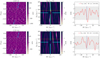 |
Fig. 10 CCF results for VI and CrI as in Fig. 9. |
| In the text | |
|
Fig. 11 Comparison between two different GIANO-B ms1d spectral orders, before (navy) and after (red) Molecfit correction. The left panel refers to the 34th spectral order, where the correction is successful. The right panel refers to the 41st spectral order, where correction does not work properly as telluric lines are saturated in this wavelength region. We did not consider the 41st spectral order and similar ones in our analyses and discarded them. |
| In the text | |
|
Fig. 12 CCF results for HCN and CO2 as in Fig. 9. At the end of the transit (phases ≃ 0.02), the noise in the CCF maps is due to the S/N drops for these exposures (see Fig. 1). |
| In the text | |
|
Fig. 13 Master-out stellar spectrum in proximity to the lithium doublet at 6707.76 Å. |
| In the text | |
|
Fig. A.1 Posterior distributions of the radial velocity analysis obtained with CaRM. |
| In the text | |
Current usage metrics show cumulative count of Article Views (full-text article views including HTML views, PDF and ePub downloads, according to the available data) and Abstracts Views on Vision4Press platform.
Data correspond to usage on the plateform after 2015. The current usage metrics is available 48-96 hours after online publication and is updated daily on week days.
Initial download of the metrics may take a while.