| Issue |
A&A
Volume 691, November 2024
Solar Orbiter First Results (Nominal Mission Phase)
|
|
|---|---|---|
| Article Number | A190 | |
| Number of page(s) | 8 | |
| Section | The Sun and the Heliosphere | |
| DOI | https://doi.org/10.1051/0004-6361/202450882 | |
| Published online | 13 November 2024 | |
High-energy insights from an escaping coronal mass ejection with Solar Orbiter/STIX observations
1
European Space Agency (ESA), European Space Research and Technology Centre (ESTEC), Keplerlaan 1, 2201 AZ Noordwijk, The Netherlands
2
University of Applied Sciences and Arts Northwestern Switzerland, Bahnhofstrasse 6, 5210 Windisch, Switzerland
3
Space Sciences Laboratory, University of California, 7 Gauss Way, 94720 Berkeley, USA
4
ETH Zürich, Rämistrasse 101, 8092 Zürich, Switzerland
⋆ Corresponding author; This email address is being protected from spambots. You need JavaScript enabled to view it.
, This email address is being protected from spambots. You need JavaScript enabled to view it.
Received:
27
May
2024
Accepted:
20
August
2024
Abstract
Context. Solar eruptive events, including solar flares and coronal mass ejections (CMEs), are typically characterised by energetically significant X-ray emissions from flare-accelerated electrons and hot thermal plasmas. However, the intense brightness of solar flares often overshadows high-coronal X-ray emissions from the associated eruptions due to the limited dynamic range of current instrumentation. Occulted events, where the main flare is blocked by the solar limb, provide an opportunity to observe and analyse the X-ray emissions specifically associated with CMEs.
Aims. This study investigates the X-ray and extreme ultraviolet (EUV) emissions associated with a large filament eruption and CME that occurred on February 15, 2022. This event was highly occulted from the three vantage points of Solar Orbiter (∼45° behind the limb), Solar–TErrestrial RElations Observatory (STEREO-A), and Earth.
Methods. We utilised X-ray observations from the Spectrometer/Telescope for Imaging X-rays (STIX) and EUV observations from the Full Sun Imager (FSI) of the Extreme Ultraviolet Imager (EUI) on board Solar Orbiter, supplemented by multi-viewpoint observations from STEREO-A/Extreme-UltraViolet Imager (EUVI). This enabled a comprehensive analysis of the X-ray emissions in relation to the filament structure observed in the EUV. We used STIX’s imaging and spectroscopy capabilities to characterise the X-ray source associated with the eruption.
Results. Our analysis reveals that the X-ray emissions associated with the occulted eruption originate from an altitude exceeding 0.3 R⊙ above the main flare site. The X-ray time profile shows a sharp increase and exponential decay, and consists of both a hot thermal component at 17 ± 2 MK and non-thermal emissions (> 11.4 ± 0.2 keV) characterised by an electron spectral index of 3.9 ± 0.2. Imaging analysis shows an extended X-ray source that coincides with the EUV emission as observed from EUI, and was imaged until the source grew to a size exceeding the STIX imaging limit (180″).
Conclusions. Filament eruptions and associated CMEs have hot and non-thermal components, and the associated X-ray emissions are energetically significant. Our findings demonstrate that STIX combined with EUI provides a unique and powerful tool for examining the energetic properties of the CME component of solar energetic eruptions. Multi-viewpoint and multi-instrument observations are crucial for revealing such energetically significant sources in solar eruptions that might otherwise remain obscured.
Key words: Sun: corona / Sun: coronal mass ejections (CMEs) / Sun: filaments / prominences / Sun: flares / Sun: X-rays / gamma rays
© The Authors 2024
 Open Access article, published by EDP Sciences, under the terms of the Creative Commons Attribution License (https://creativecommons.org/licenses/by/4.0), which permits unrestricted use, distribution, and reproduction in any medium, provided the original work is properly cited.
This article is published in open access under the Subscribe to Open model. This email address is being protected from spambots. You need JavaScript enabled to view it. to support open access publication.
1. Introduction
Solar eruptive events, which include solar flares, coronal mass ejections (CMEs), and occasionally associated solar energetic particle (SEP) events, are fundamental drivers of space weather and constitute the most energetically significant processes within our Solar System. These phenomena are driven by the rapid release of free magnetic energy in the Sun’s corona. According to the standard model of solar eruptive events, the energy release is predominantly driven by large-scale magnetic reconnection beneath an erupting magnetic flux rope or filament, leading to the flare and CME. A fundamental challenge in solar physics is understanding how this released magnetic energy is partitioned and converted into other forms, such as heat and particle acceleration.
X-ray observations of solar eruptive events provide one of the most direct diagnostics of the hottest flare plasma and the non-thermal flare-accelerated electrons. Typically in solar eruptive events, these observations reveal bright hard X-ray footpoints within the chromosphere, as well as hot flare loops rooted in these footpoints that often form an arcade in the lower corona (Fletcher et al. 2011; Benz 2017). Although it is theorised, and occasionally observed, that hard X-ray emissions also originate from higher in the corona, near the acceleration regions or in conjunction with CME eruptions, detecting these emissions presents a significant challenge. Since the intensity of bremsstrahlung X-ray emission depends on the ambient density, emission from the denser, lower solar atmosphere dominates and, given the limited dynamic range of current and past X-ray imaging instruments, usually obscures higher-altitude sources. Nevertheless, in certain exceptional circumstances (e.g. Masuda et al. 1994; Krucker & Battaglia 2014), or during times when the solar flare footpoints are occulted behind the solar limb, coronal hard X-ray emissions become detectable, offering rare glimpses into high-corona processes (e.g. Krucker & Lin 2008; Effenberger et al. 2017; Lastufka et al. 2019).
In only a handful of cases where the main flare is either fully or partially occulted by the solar limb have high-coronal hard X-ray emissions associated with CME eruptions been reported, with both Yohkoh and the Reuven Ramaty High Energy Solar Spectroscopic Imager (RHESSI) (Hudson et al. 2001; Krucker et al. 2007; Glesener et al. 2013; Lastufka et al. 2019). In these reported cases, both a non-thermal and hot thermal component of the erupting flux ropes were reported, suggesting that energetic electrons and hot plasma are present in the CME erupting filament. More recently with observations from the Expanded Owens Valley Solar Array (EOVSA), Chen et al. (2020) reported for the first time non-thermal microwave emission in the anchor points of the erupting filament, further suggesting the presence of accelerated electrons trapped within erupting flux ropes. With recent X-ray observations from the Spectrometer Telescope for Imaging X-rays (STIX) (Krucker et al. 2020) on board Solar Orbiter (Müller et al. 2020), Stiefel et al. (2023) reported the first observations on non-thermal emissions in the flux rope filament footpoints (albeit in the chromosphere), where flare-accelerated energetic electrons trapped in the flux rope presumably precipitated to the denser anchor points of the flux rope to produce X-ray emission. Understanding the nature and energetics of non-thermal emission from erupting filaments is an important aspect of understanding particle acceleration and energy release in solar eruptive events.
In this paper, we present hard X-ray observations of a filament eruption that occurred on February 15, 2022, captured by STIX and the Full Sun Imager (FSI) of the Extreme Ultraviolet Imager (EUI) on board Solar Orbiter (Rochus et al. 2020). STIX offers hard X-ray imaging and spectroscopy, measuring X-rays in the 4–150 keV energy range. Our analysis includes both the spatial and spectral aspects of the X-ray observations, revealing that the eruption exhibited both hot and non-thermal components. This work highlights the unique observational opportunities provided by STIX and other instruments on board Solar Orbiter. Section 2 presents an overview of the event, as well as more detailed X-ray imaging and spectroscopic analyses, while Sect. 1 discusses the implications of this work and provides our conclusions.
2. Observations
2.1. Event overview
On February 15, 2022, a large filament eruption took place off the eastern limb of the Sun, captured from three distinct observational vantage points: Earth, Solar–TErrestrial RElations Observatory (STEREO-A), and Solar Orbiter. The main body of the event was obscured by the solar limb from all three locations, providing a unique perspective on the eruption. Figure 1 illustrates the positions of the spacecraft relative to the Sun, and the black arrow in the figure indicates the filament eruption’s location and trajectory, determined to be ∼59° behind the limb as viewed from Earth. The eruption was captured clearly by the large field of view of the EUI/FSI telescope on board Solar Orbiter, where parts of the filament eruption were tracked out to 6 R⊙ in 304 Å (see Mierla et al. 2022). The eruption was also associated with a fast CME (∼2200 km/s) and an interplanetary CME-driven shock, which caused a widespread solar energetic particle event that was detected by in situ instruments on several spacecraft throughout the heliosphere (see Palmerio et al. 2024; Giacalone et al. 2023; Khoo et al. 2024). CMEs this fast have been known to produce hard X-ray signatures in the high corona (Krucker et al. 2007).
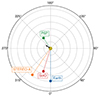 |
Fig. 1. Plot of the relative positions of Solar Orbiter, Earth, STEREO-A, and PSP at the time of the CME eruption. The black arrow marks the estimated longitude of the eruption. |
Figure 2 presents X-ray and radio measurements taken from various viewpoints during the filament eruption. Panel a demonstrates that, from Earth’s perspective, there was no detectable enhancement in X-ray emission across the channels of the GOES-16 X-Ray Sensor (XRS). Conversely, panel b shows that from the perspective of Solar Orbiter, STIX captured clear X-ray emissions reaching up to 28 keV, even though the event was also occulted behind the limb from this viewpoint. Panel c features radio observations from the Parker Solar Probe (PSP)/FIELDS (Bale et al. 2016) across both the Low Frequency Receiver (LFR; bandwidth 10.5 kHz–1.7 MHz) and the High Frequency Receiver (HFR; 1.3–19.2 MHz). During the eruption, pronounced radio bursts characteristic of Type-III signatures were detected, with their onset aligning with the peak of the X-ray emissions captured by STIX. These bursts indicate the presence of impulsively accelerated electron beams travelling from the solar atmosphere’s lower layers at the flare site into interplanetary space along open magnetic field lines. Additionally, Langmuir wave signatures were identified in the dynamic spectrum at frequencies around 0.05 MHz after approximately 22:30 UT, indicating in situ measurements of these Type-III generating electron beams by PSP, and suggesting a magnetic connection between the spacecraft and the event source.
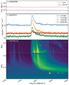 |
Fig. 2. X-ray and radio observations of the eruption as observed by Earth, Solar Orbiter, and PSP. The GOES XRS 1–8 Å and 0.5–4 Å channels are shown in panel a. The STIX light curves in four energy bands (flux summed over these energies) are shown in panel (b), where X-ray emission associated with the eruption can be seen clearly. In panel (c), the dynamic spectra observed by HFR and LFR from PSP/FIELDS are plotted, where the Type-III radio bursts associated with the event is observed. Langmuir waves are also observed at ∼0.05 MHz after around 22:20 UT. The times here are all adjusted to UT at the PSP location. |
The source region of the solar eruptive event (i.e. solar flare) was occulted from the three remote sensing viewpoints of STEREO-A, Solar Orbiter, and Earth, as depicted in Fig. 1. This is highlighted by Fig. 3, which shows the eruption as observed in the 304 Å channels of the Extreme-UltraViolet Imager (EUVI) on board STEREO-A (Wuelser et al. 2004) and Solar Orbiter/EUI/FSI. EUI’s imaging cadence at this time was 2 minutes. Therefore, each EUI image was paired with the STEREO image closest to it in time, after accounting for the different light-travel times from the eruption to the two observatories. The five frames show the filament as it comes into the field of view of both instruments, first STEREO-A/EUVI (row a) and then EUI/FSI (row b). It should be noted that the scale in arcsec difference is due to the fact that Solar Orbiter and STEREO-A are at different AU distances, at 0.72 AU and 0.96 AU, respectively. Panel c presents the STIX light curve, with vertical dashed lines correlating the timing of the frames to specific points on the light curves. A comparison of the FSI frames with the STIX light curves distinctly reveals an increase and subsequent decrease in X-ray emission as the filament eruption becomes visible in the EUI/FSI (and hence STIX) field of view, matching the CME’s outward expansion. Panel d further shows the prominence’s continued expansion and acceleration, captured by FSI’s large field of view.
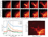 |
Fig. 3. Overview of the EUV observations in 304 Å from the different vantage points of STEREO/EUVI and Solar Orbiter/EUI/FSI. Panel (a) and panel (b) show five consecutive images from EUVI and FSI, respectively. The images of EUVI and EUI are matched to the closest time, taking light-travel time into account, and are given in the time at Solar Orbiter. They are not re-projected to one viewpoint; the maps are plotted from their respective vantage points, and hence the arcsec scales are different. The grey line in panel a shows the solar limb as viewed from Solar Orbiter. In panel (c), the STIX light curves are plotted with the five vertical lines corresponding to the five EUV images plotted in (a) and (b). In panel (d) the EUV filament eruption is shown at a later time when the X-ray emission has ceased. |
To estimate the 3D location and propagation angle of the eruption, we applied a line-of-sight triangulation technique (Ryan et al. 2024) to the isolated feature in the core of the eruption. This is clearly identifiable to both EUVI and FSI at 21:56 UT (Figs. 3a, b, fourth column). This analysis revealed that the eruption originated approximately 59° behind the solar limb as viewed from Earth–finding consistent with Mierla et al. (2022)–and about 45° behind the limb from the perspective of Solar Orbiter. Assuming the eruption propagated radially, the occultation heights are estimated at around 250 Mm. This implies that any X-ray emissions observed from Solar Orbiter must originate from an altitude exceeding 250 Mm, or at least 0.3 R⊙, above the solar limb. This supports our assertion that X-ray emission observed by STIX must originate in the filament eruption itself, as flare footpoints and the loop arcade would be too low to be visible above the limb.
The time profiles of the STIX X-ray emission show a sharp rise and an exponential decay. The time-evolution profile is due to a combination of an actual variation in the X-ray emission and an increase in the visible part of the source (see Fig. 3). The time profiles across energies are quite consistent which is highlighted further in Fig. 4, where the 4–10 keV and 12–28 keV normalised light curves are shown. The decay appears to be similar in both the thermal and non-thermal emissions (this is discussed further in Sect. 2.2), and, fitting an exponential decay to the time series, we find a decay time of τ ∼ 130 s. This is very similar, for example, to the case reported in Krucker et al. (2007). Using this value, and Eq. (2) for the collisional energy loss from Krucker et al. (2008) together with an energy of 20 keV, we can estimate the electron number density, which we find to be of the order of 108 cm−3, a reasonable value for the high corona (see more in Sect. 2.4). However, we should also note that a power-law decay also fits this decay well, with a power-law exponent of ∼3.5. The time profiles are consistent with a scenario that the X-ray source comes into view of Solar Orbiter/STIX, such that the X-ray emission rapidly increases, followed by a decay as the X-ray source expands outwards.
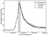 |
Fig. 4. STIX 4–10 keV and 12–28 keV time series (normalised). The grey shaded region marks the time interval over which the spectral fitting was performed. The black curve shows the exponential-decay fitted to the decay. |
As we have no direct observation of the flare associated with the eruption, we cannot estimate the GOES class of the flare. However, from the STIX observations, we can estimate the corresponding GOES class of the X-ray emission associated with the filament eruption itself. This can be done using correlations between the STIX 4–10 keV and the GOES/XRS 1–8 Å channel of historically observed events (Xiao et al. 2023). This gives the GOES class of the peak emission from the filament as between a B6 and C.1 flare. However, it should be noted that this correlation relationship between the GOES/XRS X-ray flux and STIX flux is based upon regular flares rather than X-ray emissions associated with a CME, so it is not necessarily clear if this correlation should hold for the case of this observation. For example, if the temperature of the source is very high, it would give a relatively low GOES class due to the differences in the GOES/XRS and STIX temperature responses. If instead we use the temperature and emission measure from the fit of the STIX spectra (see Sect. 2.2), the estimated GOES class from these parameters is that of an A4 GOES-class flare. However, we note here that this value is a lower limit of the estimated equivalent GOES class of the high-coronal X-ray source, as it only contains the hottest temperatures within the STIX sensitivity range, and most likely there are also contributions from the ‘cooler’ plasma within the GOES/XRS sensitivity range, but for which we do not have observations. In either case, we note that fluxes of this event observed by STIX are at a substantial emission level, given the eruption’s separation from the main flaring site behind the limb, whereas had the event not been occulted, this emission would not have been distinguishable amid the much brighter flare emission.
2.2. X-ray spectral analysis
In order to determine the nature of the coronal X-ray emission observed by STIX, we conducted spectral analysis focusing on the peak of the X-ray emission. The time interval used here is within the grey shaded region in Fig. 4, during the peak minute from 21:52:29–21:53:32 UT, ensuring a sufficient count rate for analysis. The background-subtracted1 spectrum was then fitted using OSPEX (Tolbert & Schwartz 2020). The spectrum is represented by an isothermal model (f_vth) combined with a thin-target non-thermal model (f_thin2) fitted over an energy range of 4–28 keV. We attempted to fit different models to the data, including a super-hot component, and combinations of thick-target and thermal components, but find that the isothermal and non-thermal thin-target combination of models fit the best. The results of the fit are shown in Fig. 5, where the background-subtracted X-ray count spectrum is plotted in black, and the thermal and non-thermal models are shown in red and blue, respectively. The vertical dashed lines show the energy range over which the spectrum was fitted, and the bottom panel shows the residuals of the fit to the data. Below approximately 10 keV, thermal emission is dominant, with the fit indicating a low energy cutoff at 11.4 ± 0.4 keV. The spectra also reveal a pronounced non-thermal component, characterised by an electron spectral index (δ) of 3.9 ± 0.2. The fit of the thermal component suggests a high temperature of 17 ± 2 MK and a relatively low emission measure of 1.36 ± 0.56 × 1046 cm−3, consistent with the emitting plasma being a hot, diffuse X-ray emitting source.
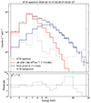 |
Fig. 5. STIX background-subtracted X-ray count flux spectra (black) over the peak of the X-ray emission, and the fitting results. The isothermal fit is plotted in red, and the non-thermal thin-target model is plotted in blue. Below the spectrum are the residuals of the fit to the data. The vertical dashed lines mark the energy range over which the spectral fit was performed. |
2.3. X-ray imaging
STIX is an indirect Fourier imager and uses a grid-based approach to reconstruct images from spatial modulation patterns of the incident X-ray flux on the detectors (Krucker et al. 2020; Massa et al. 2023). The instrument is designed such that the grid pitches and orientations provide spatial information on angular scales on the Sun of 7″–180″. To generate images from STIX visibilities, significant flux and signal modulations are required from each sub-collimator. Utilising the forward fit algorithm (FWDFIT; Volpara et al. 2022), we constructed a sequence of thermal X-ray images with 30-second integration in the 4–10 keV range during the peak X-ray emissions. Modulations were primarily detected in the coarsest grids (sub-collimators 7–10), indicating an extended source size, which were then employed for image construction. For each time interval, the CLEAN algorithm was also used to construct the X-ray source images, adopting a clean beam width of 60″, corresponding to the resolution of the finest grids used (i.e. sub-collimator 7).
Figure 6 presents the reconstructed STIX thermal X-ray images across five intervals at the X-ray emission peak in the top panel. For the two time intervals for which a corresponding EUI/FSI map is available, the map is plotted directly beneath. The CLEAN reconstructed maps are denoted by the green colour map and contours at each time step, with the forward-fit map full width half maximum (FWHM) represented by a black circle. The dashed black circle delineates the 180″ boundary limit of the coarsest STIX sub-collimator. The observed thermal X-ray source in the 4–10 keV energy range is large and extended, aligning with the filament eruption’s entry into Solar Orbiter’s field of view. The FWDFIT FWHM indicates the source’s growth and outward movement, reaching the 180″ limit of the coarsest sub-collimator, as visible in the final panel. After this time, we cannot reliably construct an image with STIX, as the source is too extended. The CLEAN maps show an evolution of the source that similarly follows the FWDFIT maps, but also shows the structure as it evolves, which appears to track the legs of the filament eruption. We find a similar morphology using the MEM_GE imaging algorithm. Given the limited temporal resolution of EUI/FSI, we can only compare the time the source comes into view and then, notably in the last panel, where the thermal source mirrors the EUV structure’s brightest ‘arm’ feature, suggesting that the bright emission in the EUV 304 Å also has a hot thermal component as evidenced by the STIX X-ray source. For the last panel, we shifted the STIX image in this frame by (40″, 20 ″) to match the brightest sources of the EUV emission. This is similarly observed in the FSI 174 Å channel.
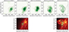 |
Fig. 6. Time evolution of the X-ray 4–10 keV source during the peak of the X-ray emission. The top panel shows the STIX images reconstructed using the CLEAN algorithm with a 30 s time integration. The green colour map and green contours show the CLEAN intensity maps, scaled to the peak flux, and the contours show the 40–100% levels. The black circle marks the FWHM of the FWDFIT-reconstructed maps over the same time intervals, and the dashed black circle marks the 180″ limit. The corresponding EUI/FSI maps for the two time intervals for which observations are available are plotted below, with the STIX contours over-plotted on top. To over-plot these STIX images on the corresponding EUI/FSI maps, the contours were over-plotted using the ‘SphericalScreen’ context manager available through the sunpy package. For the right-most panel, the STIX contours are shifted by (40″, 20″) to better align with the EUV emission based on the brightest sources. |
For the non-thermal emissions, we chose an energy range from 12–28 keV to construct an image. This was chosen because the fitted count spectrum shows that the energy range from 12–28 keV is largely non-thermal. Given that the count statistics are lower relative to the thermal X-ray source, we used a longer integration time of 1 minute over the peak of the light curve to construct an image. For reference, we also constructed a thermal source image in the 4–10 keV over the same time range interval. We applied FWDFIT to obtain estimates of the positions and sizes of both the thermal and non-thermal sources during the peak X-ray emission. Figure 7 displays these, with the 12–28 keV non-thermal source outlined in blue contours and the 4–10 keV thermal source in red. These contours were over-plotted on a running difference image from EUI/FSI at 174 Å, which distinctly shows the CME shock front or the leading edge of the CME, prominently visible well above the filament eruption and the X-ray sources. According to the forward-fit results, the thermal source exhibits a FWHM of 110 ± 16″ while the non-thermal source measures 76 ± 17″. Although their locations diverge slightly, pinpointing their precise positions relative to the filament eruption and its orientation presents a challenge. However, it seems that both sources are situated within the ‘legs’ of the filament as it enters Solar Orbiter’s field of view.
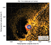 |
Fig. 7. Non-thermal 12–28 keV (blue) and thermal 4–10 keV (red) forward-fit X-ray sources over the peak of the X-ray emission, over-plotted on the running difference EUV 174 Å image from EUI/FSI. |
2.4. Energetics of the X-ray sources
Combining the parameters derived from the X-ray spectral fitting and X-ray imaging, we could estimate the thermal source properties. We determined the volume of the X-ray emitting thermal plasma through the forward fitting of the circular source over the peak of the emission from Fig. 3. After using the FWDFIT source to estimate the volume, we also tested the method using CLEAN maps by estimating the area within the 30% contour levels and found a similar volume estimate. We then estimated the ambient density, ne of the thermal source by combining with the emission measure (EM) derived from the spectral fit,
![Mathematical equation: $$ \begin{aligned} n_e = \sqrt{\frac{\mathrm{EM}}{V}}\,\, \mathrm [cm^{-3}] . \end{aligned} $$](/articles/aa/full_html/2024/11/aa50882-24/aa50882-24-eq1.gif) (1)
(1)
If we assume the simple approach that the thermal source is spherically symmetric with a filling factor of one, (i.e. V = fV, where f < 1), the derived density of the hot (17 MK) plasma source is ∼3.7 × 108 cm−3, which is a reasonable value for CME high in the corona. This source hence contains around 3.8 × 1037 electrons and has an estimated thermal energy content of ∼2.7 × 1029 erg. We emphasise that these values are estimates, not definitive values. The largest uncertainty in these calculations is the volume estimate. If we use the ranges of volumes given from the uncertainties in the source size, we obtain the following ranges: ne between (3–4.7)×108 cm−3, the number of electrons in the thermal source between (3–4.6)×1037, and the thermal energy content between 2.1–3.2 ergs.
For the non-thermal emission, we can estimate the instantaneous electron density and number of non-thermal electrons. For a thin-target model, this can be estimated by using Eq. (6) from Kontar et al. (2023), (see also Appendix B in Musset et al. 2018), given by
![Mathematical equation: $$ \begin{aligned} n_{\rm nth} = \frac{\langle n V F_0 \rangle }{n V_{\rm nth}} E_0^{-0.5} \frac{\delta -1}{\delta -0.5} \sqrt{\frac{m_e}{2}}\,\, \mathrm [cm^{-3}] , \end{aligned} $$](/articles/aa/full_html/2024/11/aa50882-24/aa50882-24-eq2.gif) (2)
(2)
where n is the ambient density, ⟨nVF0⟩ and δ are the normalisation factor and the electron spectral index from the thin-target model fit, respectively, E0 is the low energy cut-off, Vnth is the non-thermal source volume, and me is the electron mass in keV/c2. From the spectral fit in Sect. 2.2 we use the parameters obtained; ⟨nVF0⟩ = 1.86 × 1054 electrons s−1 cm−2, δthin = 3.9, and Ec = 11.4 keV. We use the volume estimate from Sect. 2.3, Vnth ∼ 3 × 1028 cm3, assuming a spherically symmetric source with a filling factor of unity. As the ambient density is not well-constrained, and nor is the low-energy cut-off, we could plot the instantaneous non-thermal electron density for a range of ambient densities and low-energy cutoffs, in a manner similar to that in Lastufka et al. (2019). For a range of ambient densities, we only calculated the instantaneous non-thermal electron density for values for which the thin-target assumption holds (i.e. the ambient density does not act as a thick target). To determine the high densities for which the assumption does not hold, we calculated the stopping column densities for different cut-off energies using the estimated source size from Sect. 2.3, and Eq. (1) from Krucker et al. (2008). In Fig. 8, this is shown for three ranges of the Ec, namely 6 keV, 11.4 keV, and 20 keV. The shaded regions note the ranges of values for the non-thermal volume estimate, Vnt. The solid grey line shows the extreme case when the ambient density equals the non-thermal density, and the dashed grey lines show the cases when the non-thermal density is 10% and 1% of ambient density. If we take the ambient density, n, to be that of the thermal source (∼3.7 × 108 cm−3), we get an estimated nnth ∼ 2 × 107 cm−3 (marked by the black star in Fig 8). With these assumptions, we find that the ratio of the non-thermal to thermal electron density is ≃0.05. Under these assumptions, that the ambient density is the thermal source, we find a total number of non-thermal electrons of ∼7 × 1035, which is approximately 2% of the total population of electrons, and a total energy content of the non-thermal source to be ∼2 × 1028 erg. This is approximately 7% of the estimated thermal energy. Similar to the thermal source estimates, if we take the ranges of the volume estimates for the non-thermal source, we find that the total number of non-thermal electrons ranges from (5.3–8.3)×1035, and the total energy ranges from (1.5–2.3)×1028 ergs.
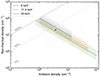 |
Fig. 8. Plot of the instantaneous non-thermal electron density as a function of ambient density for three different low-energy cut-offs. The non-thermal electron density is calculated and plotted only where the thin-target assumption is valid. The shaded regions mark the ranges of the estimated volume from the source size estimations. The grey lines at 100%, 10%, and 1% mark where the ambient density equals the respective percentages of the non-thermal density (i.e. 100% is the extreme cases when the ambient density equals the non-thermal electron density.) The black star marks the value of the instantaneous non-thermal electron density if we assume the ambient density is that of the thermal source. |
3. Discussion and conclusion
The large filament eruption and CME that occurred on February 15, 2022, provided an excellent opportunity to study an occulted solar eruptive event from the perspective of Solar Orbiter. By combining STIX and multi-viewpoint EUV observations from both EUI/FSI and STEREO-A/EUVI, this study reveals the existence of a hot (> 17 MK) X-ray component and the presence of flare-accelerated non-thermal electrons within the coronal source, associated with a filament eruption located at least 250 Mm radially above the main flare site. The X-ray time profile is relatively simple: it peaks as the filament comes into view of Solar Orbiter, as identified in the EUV from EUI/FSI, and shows an exponential decay on the timescale of ∼130 s. The X-ray source was imaged over the peak of the emission, and shows a source that spatially aligns with the EUV structure as seen in the 304 Å and 174 Å channels of EUI/FSI, and grows in size until it reaches the detection limit of STIX’s largest grids of 180″, beyond which an X-ray image cannot be reconstructed as it is too extended to show any modulation even in the coarsest STIX grids. The presence of the hard X-ray non-thermal emissions above 11 keV, with an electron spectral index of 3.9 ± 0.2 keV, suggest that there is a population of accelerated electrons that are confined to magnetic field line structures associated with the CME and filament eruption, likely situated in the legs of the filament eruption that is observed in the EUV, behind the CME shock.
We then consider how the X-ray emitting plasma of the filament reached temperatures as high as 17 MK, and how a population of accelerated electrons became embedded within this structure at these altitudes. A likely scenario, based on a 3D eruptive flare model (e.g. Janvier et al. 2015), is that flare-accelerated electrons escaping upwards from the acceleration region near the current sheet are injected into the complex magnetic configuration of the filament. Within this structure, they are then trapped and carried outwards with the erupting filament. Recent observations have documented similar processes at lower altitudes: microwave emission from accelerated electrons at the conjugate legs of a filament eruption (Chen et al. 2020) and hard X-ray detection at the filament anchor points in the chromosphere (Stiefel et al. 2023). This study extends those findings to their coronal counterparts, suggesting that these electrons can remain trapped within the filament structure for an extended duration, observable at these higher altitudes. It should also be noted that the detection of Type-III radio bursts indicates that some flare-accelerated electrons have also escaped upwards onto open magnetic field lines, as well as those that access the confined magnetic structure.
The hot thermal X-ray sources match the structure observed in the EUV channels of EUI/FSI, and are similarly seen in the other hotter coronal channels from EUVI (see Fig. 5 in Mierla et al. 2022). Although the FSI 304 Å passband is typically dominated by He II 304 Å, it also contains hotter lines indicative of temperatures around 2 MK, and the FSI 174 Å channel has a peak temperature response at approximately 1 MK. These observations suggest that the filament exhibits a multi-thermal distribution and is significantly heated. The heating of the flux rope to temperatures of up to tens of milli-Kelvins could be attributed to flare-accelerated electrons heating the CME filament, a mechanism that has been proposed in similar studies (see Glesener et al. 2013). We strongly encourage modellers to further investigate the injection of accelerated electrons into different plasma conditions (Galloway et al. 2010) and in particular, the injection in CMEs structures. This will allow us to understand the production of bremsstrahlung emission from these scenarios.
The observed time profiles of both thermal and non-thermal X-ray emissions, characterised by a sharp rise followed by an exponential decay, also offers insights that improve our understanding of the nature of the sources. Typically, in emission associated with a solar flare, one would expect the non-thermal emissions to peak sharply and decay rapidly, preceding the thermal emissions, which would peak later and decay more gradually. However, in this case, both the thermal and non-thermal emissions exhibit similarly structured profiles and decay rates. The non-thermal decay could be explained by collisional losses; however, different energy levels would likely exhibit varying decay times under such a scenario. Another plausible explanation is that as the emitting source moves outwards, the ambient density decreases, leading to a flux decay. Since both thin-target and thermal bremsstrahlung emissions are dependent on ambient density, an isotropic expansion of the emitting volume would naturally result in a decrease in emission over time, proportional to the cube of the expansion time, which aligns with our observations. In this way, the observations of the initial sharp rise in X-ray emissions are due to the emitting volume moving into Solar Orbiter’s field of view from behind the limb. Once fully observable by STIX, the source continues to expand outwards, leading to the observed decay in emission. This can also explain the absence of detectable X-ray emissions when the event becomes visible from Earth; by this stage, the expanded volume would be too diffuse, such that the emission would be below the detection threshold of GOES/XRS. In reality, both collisional losses and the expansion are at play, but overall, the observations show a consistent picture of hot plasma and trapped non-thermal electrons within a filament structure. The non-thermal population observed is a lower limit of the total electrons in the high-altitude source, and there may have been more at earlier altitudes that could have contributed to the heating of the structure. This study shows that while the emission is weak, it is still energetically significant, and this work is important for understanding how the energy budget is utilised in solar eruptive events.
Future work will leverage STIX observations in conjunction with Earth-based observatories, including the newly operational Hard X-ray Imager (HXI; Zhang et al. 2019) on board ASO-S (Gan et al. 2019), the Gamma-ray Burst Monitor (GBM) (Meegan et al. 2009) and Aditya-HEL1OS, in order to systematically search for solar eruptive events from multiple vantage points that can be studied. This approach will enable us to identify configurations where the main flare is occulted from one viewpoint but visible from another. Such multi-viewpoint observations will allow simultaneous X-ray analyses of both the flare and the coronal CME component, providing a comprehensive view of the high-energy aspects of solar eruptive events. In addition, we will attempt to search for events that occur during the perihelion of PSP, such that PSP measures the in situ aspect energetic electrons of the CME very close to the Sun, which could be compared with the remote sensing X-ray observations.
While this study demonstrates the capability of STIX to measure coronal X-ray emissions associated with a CME, the identification of the source was facilitated by the fact that the main flare was occulted behind the limb. The use of indirect Fourier imagers such as STIX are inherently limited by the dynamic range of the observations, requiring reliance on occulted events–where the bright flare source is obscured–to detect coronal X-rays. Looking to the future, the adoption of a direct X-ray imager, such as FOXSI (Christe et al. 2023; Glesener et al. 2023), which has been proposed as part of the FIERCE (Shih et al. 2023) and SPARK (Reid et al. 2023) mission concepts, would revolutionise our observational approach. A direct imager would allow for simultaneous imaging of both the flare and the coronal emission, substantially improving our understanding of the complex dynamics of solar eruptive events, and allow us to identify the locations of particle acceleration and heating and whether electron acceleration occurs in the current sheet below the CME or within the CME itself.
Background file from quiet period on 2022-02-16, UID: 2202160007.
Acknowledgments
Solar Orbiter is a space mission of international collaboration between ESA and NASA, operated by ESA. The STIX instrument is an international collaboration between Switzerland, Poland, France, Czech Republic, Germany, Austria, Ireland, and Italy. L.A.H is supported by an ESA Research Fellowship. S.K. and H.C. are supported by the Swiss National Science Foundation Grant 200021L_189180 for STIX. This paper made use of several open source packages including astropy (Astropy Collaboration 2022), sunpy (The SunPy Community 2020; Mumford et al. 2020), matplotlib (Hunter 2007), numpy (Harris et al. 2020), scipy (Virtanen et al. 2020), pandas (pandas development team 2020), sunpy-soar. The IDL software used in this work used the SSW packages, and version v0.5.3 of the STIX software. See also https://github.com/i4Ds/STIX-GSW. The authors thanks the anonymous referee for their helpful comments which improved this manuscript.
References
- Astropy Collaboration (Price-Whelan, A. M., et al.) 2022, ApJ, 935, 167 [NASA ADS] [CrossRef] [Google Scholar]
- Bale, S. D., Goetz, K., Harvey, P. R., et al. 2016, Space Sci. Rev., 204, 49 [Google Scholar]
- Benz, A. O. 2017, Liv. Rev. Sol. Phys., 14, 2 [Google Scholar]
- Chen, B., Yu, S., Reeves, K. K., & Gary, D. E. 2020, ApJ, 895, L50 [NASA ADS] [CrossRef] [Google Scholar]
- Christe, S., Alaoui, M., Allred, J., et al. 2023, BAAS, 55, 065 [NASA ADS] [Google Scholar]
- Effenberger, F., Rubio da Costa, F., Oka, M., et al. 2017, ApJ, 835, 124 [NASA ADS] [CrossRef] [Google Scholar]
- Fletcher, L., Dennis, B. R., Hudson, H. S., et al. 2011, Space Sci. Rev., 159, 19 [Google Scholar]
- Galloway, R. K., Helander, P., MacKinnon, A. L., & Brown, J. C. 2010, A&A, 520, A72 [NASA ADS] [CrossRef] [EDP Sciences] [Google Scholar]
- Gan, W.-Q., Zhu, C., Deng, Y.-Y., et al. 2019, Res. Astron. Astrophys., 19, 156 [Google Scholar]
- Giacalone, J., Cohen, C. M. S., McComas, D. J., et al. 2023, ApJ, 958, 144 [NASA ADS] [CrossRef] [Google Scholar]
- Glesener, L., Krucker, S., Bain, H. M., & Lin, R. P. 2013, ApJ, 779, L29 [NASA ADS] [CrossRef] [Google Scholar]
- Glesener, L., Shih, A. Y., Caspi, A., et al. 2023, BAAS, 55, 129 [NASA ADS] [Google Scholar]
- Harris, C. R., Millman, K. J., van der Walt, S. J., et al. 2020, Nature, 585, 357 [NASA ADS] [CrossRef] [Google Scholar]
- Hudson, H. S., Kosugi, T., Nitta, N. V., & Shimojo, M. 2001, ApJ, 561, L211 [NASA ADS] [CrossRef] [Google Scholar]
- Hunter, J. D. 2007, Comput. Sci. Eng., 9, 90 [NASA ADS] [CrossRef] [Google Scholar]
- Janvier, M., Aulanier, G., & Démoulin, P. 2015, Sol. Phys., 290, 3425 [Google Scholar]
- Khoo, L. Y., Sánchez-Cano, B., Lee, C. O., et al. 2024, ApJ, 963, 107 [NASA ADS] [CrossRef] [Google Scholar]
- Kontar, E. P., Emslie, A. G., Motorina, G. G., & Dennis, B. R. 2023, ApJ, 947, L13 [NASA ADS] [CrossRef] [Google Scholar]
- Krucker, S., & Battaglia, M. 2014, ApJ, 780, 107 [Google Scholar]
- Krucker, S., & Lin, R. P. 2008, ApJ, 673, 1181 [NASA ADS] [CrossRef] [Google Scholar]
- Krucker, S., White, S. M., & Lin, R. P. 2007, ApJ, 669, L49 [NASA ADS] [CrossRef] [Google Scholar]
- Krucker, S., Battaglia, M., Cargill, P. J., et al. 2008, A&ARv, 16, 155 [NASA ADS] [CrossRef] [Google Scholar]
- Krucker, S., Hurford, G. J., Grimm, O., et al. 2020, A&A, 642, A15 [NASA ADS] [CrossRef] [EDP Sciences] [Google Scholar]
- Lastufka, E., Krucker, S., Zimovets, I., et al. 2019, ApJ, 886, 9 [NASA ADS] [CrossRef] [Google Scholar]
- Massa, P., Hurford, G. J., Volpara, A., et al. 2023, Sol. Phys., 298, 114 [NASA ADS] [CrossRef] [Google Scholar]
- Masuda, S., Kosugi, T., Hara, H., Tsuneta, S., & Ogawara, Y. 1994, Nature, 371, 495 [CrossRef] [Google Scholar]
- Meegan, C., Lichti, G., Bhat, P. N., et al. 2009, ApJ, 702, 791 [Google Scholar]
- Mierla, M., Zhukov, A. N., Berghmans, D., et al. 2022, A&A, 662, L5 [NASA ADS] [CrossRef] [EDP Sciences] [Google Scholar]
- Müller, D., St. Cyr, O. C., Zouganelis, I., et al. 2020, A&A, 642, A1 [Google Scholar]
- Mumford, S., Freij, N., Christe, S., et al. 2020, J. Open Source Softw., 5, 1832 [NASA ADS] [CrossRef] [Google Scholar]
- Musset, S., Kontar, E. P., & Vilmer, N. 2018, A&A, 610, A6 [NASA ADS] [CrossRef] [EDP Sciences] [Google Scholar]
- Palmerio, E., Carcaboso, F., Khoo, L. Y., et al. 2024, ApJ, 963, 108 [NASA ADS] [CrossRef] [Google Scholar]
- pandas development team 2020, https://doi.org/10.5281/zenodo.3509134 [Google Scholar]
- Reid, H. A. S., Musset, S., Ryan, D. F., et al. 2023, Aerospace, 10, 1034 [NASA ADS] [CrossRef] [Google Scholar]
- Rochus, P., Auchère, F., Berghmans, D., et al. 2020, A&A, 642, A8 [NASA ADS] [CrossRef] [EDP Sciences] [Google Scholar]
- Ryan, D. F., Laube, S., Nicula, B., et al. 2024, A&A, 681, A61 (SO Nominal Mission Phase SI) [NASA ADS] [CrossRef] [EDP Sciences] [Google Scholar]
- Shih, A. Y., Glesener, L., Krucker, S., et al. 2023, BAAS, 55, 364 [NASA ADS] [Google Scholar]
- Stiefel, M. Z., Battaglia, A. F., Barczynski, K., et al. 2023, A&A, 670, A89 [NASA ADS] [CrossRef] [EDP Sciences] [Google Scholar]
- The SunPy Community (Barnes, W. T., et al.) 2020, ApJ, 890, 68 [Google Scholar]
- Tolbert, K., & Schwartz, R. 2020, Astrophysics Source Code Library [record ascl: 2007.018] [Google Scholar]
- Virtanen, P., Gommers, R., Oliphant, T. E., et al. 2020, Nat. Meth., 17, 261 [Google Scholar]
- Volpara, A., Massa, P., Perracchione, E., et al. 2022, A&A, 668, A145 [NASA ADS] [CrossRef] [EDP Sciences] [Google Scholar]
- Wuelser, J.-P., Lemen, J. R., Tarbell, T. D., et al. 2004, SPIE Conf. Ser., 5171, 111 [Google Scholar]
- Xiao, H., Maloney, S., Krucker, S., et al. 2023, A&A, 673, A142 (SO Nominal Mission Phase SI) [NASA ADS] [CrossRef] [EDP Sciences] [Google Scholar]
- Zhang, Z., Chen, D.-Y., Wu, J., et al. 2019, Res. Astron. Astrophys., 19, 160 [CrossRef] [Google Scholar]
All Figures
|
Fig. 1. Plot of the relative positions of Solar Orbiter, Earth, STEREO-A, and PSP at the time of the CME eruption. The black arrow marks the estimated longitude of the eruption. |
| In the text | |
|
Fig. 2. X-ray and radio observations of the eruption as observed by Earth, Solar Orbiter, and PSP. The GOES XRS 1–8 Å and 0.5–4 Å channels are shown in panel a. The STIX light curves in four energy bands (flux summed over these energies) are shown in panel (b), where X-ray emission associated with the eruption can be seen clearly. In panel (c), the dynamic spectra observed by HFR and LFR from PSP/FIELDS are plotted, where the Type-III radio bursts associated with the event is observed. Langmuir waves are also observed at ∼0.05 MHz after around 22:20 UT. The times here are all adjusted to UT at the PSP location. |
| In the text | |
|
Fig. 3. Overview of the EUV observations in 304 Å from the different vantage points of STEREO/EUVI and Solar Orbiter/EUI/FSI. Panel (a) and panel (b) show five consecutive images from EUVI and FSI, respectively. The images of EUVI and EUI are matched to the closest time, taking light-travel time into account, and are given in the time at Solar Orbiter. They are not re-projected to one viewpoint; the maps are plotted from their respective vantage points, and hence the arcsec scales are different. The grey line in panel a shows the solar limb as viewed from Solar Orbiter. In panel (c), the STIX light curves are plotted with the five vertical lines corresponding to the five EUV images plotted in (a) and (b). In panel (d) the EUV filament eruption is shown at a later time when the X-ray emission has ceased. |
| In the text | |
|
Fig. 4. STIX 4–10 keV and 12–28 keV time series (normalised). The grey shaded region marks the time interval over which the spectral fitting was performed. The black curve shows the exponential-decay fitted to the decay. |
| In the text | |
|
Fig. 5. STIX background-subtracted X-ray count flux spectra (black) over the peak of the X-ray emission, and the fitting results. The isothermal fit is plotted in red, and the non-thermal thin-target model is plotted in blue. Below the spectrum are the residuals of the fit to the data. The vertical dashed lines mark the energy range over which the spectral fit was performed. |
| In the text | |
|
Fig. 6. Time evolution of the X-ray 4–10 keV source during the peak of the X-ray emission. The top panel shows the STIX images reconstructed using the CLEAN algorithm with a 30 s time integration. The green colour map and green contours show the CLEAN intensity maps, scaled to the peak flux, and the contours show the 40–100% levels. The black circle marks the FWHM of the FWDFIT-reconstructed maps over the same time intervals, and the dashed black circle marks the 180″ limit. The corresponding EUI/FSI maps for the two time intervals for which observations are available are plotted below, with the STIX contours over-plotted on top. To over-plot these STIX images on the corresponding EUI/FSI maps, the contours were over-plotted using the ‘SphericalScreen’ context manager available through the sunpy package. For the right-most panel, the STIX contours are shifted by (40″, 20″) to better align with the EUV emission based on the brightest sources. |
| In the text | |
|
Fig. 7. Non-thermal 12–28 keV (blue) and thermal 4–10 keV (red) forward-fit X-ray sources over the peak of the X-ray emission, over-plotted on the running difference EUV 174 Å image from EUI/FSI. |
| In the text | |
|
Fig. 8. Plot of the instantaneous non-thermal electron density as a function of ambient density for three different low-energy cut-offs. The non-thermal electron density is calculated and plotted only where the thin-target assumption is valid. The shaded regions mark the ranges of the estimated volume from the source size estimations. The grey lines at 100%, 10%, and 1% mark where the ambient density equals the respective percentages of the non-thermal density (i.e. 100% is the extreme cases when the ambient density equals the non-thermal electron density.) The black star marks the value of the instantaneous non-thermal electron density if we assume the ambient density is that of the thermal source. |
| In the text | |
Current usage metrics show cumulative count of Article Views (full-text article views including HTML views, PDF and ePub downloads, according to the available data) and Abstracts Views on Vision4Press platform.
Data correspond to usage on the plateform after 2015. The current usage metrics is available 48-96 hours after online publication and is updated daily on week days.
Initial download of the metrics may take a while.