| Issue |
A&A
Volume 691, November 2024
|
|
|---|---|---|
| Article Number | A274 | |
| Number of page(s) | 12 | |
| Section | The Sun and the Heliosphere | |
| DOI | https://doi.org/10.1051/0004-6361/202450625 | |
| Published online | 19 November 2024 | |
Abnormal Stokes V profiles observed by Hinode in a sunspot
Detection of hidden photospheric fine-structures
1
Physics Department, Faculty of Science, Imam Khomeini International University, Qazvin 34149-16818, Islamic Republic of Iran
2
Physics Department, Sharif University of Technology, Tehran P.O. 11365-9161, Islamic Republic of Iran
⋆ Corresponding authors; This email address is being protected from spambots. You need JavaScript enabled to view it.
, This email address is being protected from spambots. You need JavaScript enabled to view it.
Received:
6
May
2024
Accepted:
26
September
2024
Abstract
Context. Hidden magnetic components in a sunspot are present as small-scale structures that are absent in low-resolution observations.
Aims. We search for traces of the hidden magnetic components in spectro-polarimetric observations of a mature sunspot close to the disk center recorded by Hinode.
Methods. To find extra humps in the far blue and red lobes of Stokes V, we examined the sign reversal in the second derivative of the profile in the umbra and penumbra. We also looked for the hump signature in the Stokes I and the linear polarization profiles.
Results. The amplitudes of the humps are small compared to the main component. More than half of the profiles show one extra hump, while 21% show an extra hump on both the blue and the red lobe of the 630.15 nm line with the same magnetic polarity as the sunspot. The location of the pixels where the extra hump is seen on both lobes has a pseudo-grainy structure in the single wavelength Stokes V magnetograms. This type of profile is better detected in darker parts of the penumbra, as well as in the umbra-penumbra border toward the umbra. The spectral distance between the two humps averaged over elliptical rings levels off in the umbra, decreases toward the penumbra, and levels off again there. We find no correlations between the wavelength positions of the two humps.
Conclusions. We discuss two scenarios that could potentially produce the simultaneously observed blue and red humps: one in which a single hidden magnetic component is responsible for the two humps, and another in which the two humps emanate from two hidden magnetic components.
Key words: line: profiles / polarization / Sun: magnetic fields / sunspots
© The Authors 2024
 Open Access article, published by EDP Sciences, under the terms of the Creative Commons Attribution License (https://creativecommons.org/licenses/by/4.0), which permits unrestricted use, distribution, and reproduction in any medium, provided the original work is properly cited.
This article is published in open access under the Subscribe to Open model. This email address is being protected from spambots. You need JavaScript enabled to view it. to support open access publication.
1. Introduction
Sunspots are the largest magnetic structures in the solar photosphere. They harbor a dark umbra surrounded by a brighter filamentary penumbra. The minimum intensity of the largest umbrae in the photosphere is about 5% of the average intensity of the quiet Sun. The penumbral continuum intensity is to a large extent constant and independent of sunspot size. The Evershed flow, which was observed in the photospheric layer of the penumbra, has been the subject of rigorous investigation by many authors since its discovery (Solanki 2003; Thomas & Weiss 2004; Borrero & Ichimoto 2011). Different modes of magneto-convection operate in the umbra and penumbra (Scharmer & Spruit 2006; Rempel & Schlichenmaier 2011). The magnetic field lines are close to vertical in the umbra, while they are horizontal at the penumbra border. Therefore, the penumbra phenomena have been rigorously discussed as magnetoconvection in strongly inclined magnetic fields (Schlichenmaier et al. 1998; Scharmer 2009).
Stokes profiles in quiet Sun regions show a degree of asymmetry, the primary driver of which is convective motions in granulations. As discussed by Sánchez Almeida & Lites (1992) as well as Steiner (2000), gradients in the line-of-sight velocity and/or in the magnetic field strength or inclination are responsible for generating asymmetric Stokes V profiles, including single-lobe and Q-like profiles. Due to the Evershed flow in sunspot penumbra, systematically asymmetric Stokes V profiles are observed in both visible and near-infrared (NIR) wavelengths (Sánchez Almeida & Lites 1992; Martínez Pillet et al. 1997; Schlichenmaier & Collados 2002).
Stokes profiles with opposite polarities have been observed in and around sunspots. In particular, using Hinode data, Franz & Schlichenmaier (2009) reported evidence for opposite-polarity Stokes V profiles within the penumbra. In addition, Katsukawa & Jurčák (2010) reported different kinds of patchy enhancements visible in the far red or blue wing Stokes V maps of the penumbra. These Stokes V profiles are characterized by the presence of humps on the blue or red wing (see also, e.g., Shimizu et al. 2008; Sainz Dalda & Bellot Rubio 2008).
The physical processes leading to the stability and decay of a sunspot depend largely on its subphotospheric structure, which notably must leave fingerprints in the photospheric structure. In this context, the Stokes parameters are a commonly used photospheric diagnostic tool. In this study, we analyzed a data set from spectro-polarimetric observations of photospheric spectral lines in a sunspot. Motivated by Katsukawa & Jurčák (2010), we searched for traces of abnormal Stokes V profiles. We applied an identification procedure to detect the abnormal Stokes V profiles that have one or more extra humps. We find different categories of Stokes V profiles with extra hump(s) in the blue and/or red wings of the neutral iron lines at 630 nm and discuss the statistics of their intensities, Doppler shifts, and asymmetries, focusing on profiles with an extra hump on both the blue and the red lobes newly identified and detected by Hamedivafa (2023). We then discuss possible scenarios to explain both extra humps as the signature of hidden magnetic structures. It is well known that large Stokes V signals correspond to small asymmetries (Sigwarth 2001). We also examine the amplitude asymmetry of Stokes V profiles in order to trace these hidden structures.
2. Data set and data reduction
In order to find the regions of the penumbra that show large Doppler velocities (probably in deep layers) in the photosphere, we studied the Stokes V profiles recorded by Hinode Solar Optical Telescope (SOT, Tsuneta et al. 2008; Suematsu et al. 2008) in two neutral iron spectral lines around 630 nm. In each pixel, we investigated the shape of the Stokes V profiles in the penumbra and parts of the umbra of the sunspot in active region NOAA 10944. At the time of observation, 28 February 2007 from 17:57 to 18:41 UT, this sunspot was located very close to the solar disk center (the center of the spot was located at 12″ W and 8″ N, μ = 1.00).
The spectro-polarimeter (SP) on board Hinode records the full Stokes parameters in two spectral lines of neutral iron at 630.15 and 630.25 nm (hereafter, we refer to them as the first and second spectral lines, respectively). The spectral sampling of this SP is 21.5 mÅ and 56 wavelength points were recorded around each spectral line for each Stokes parameter (112 wavelength points in total). The spatial samplings in the horizontal and vertical directions are 0.15 and 0.16 arcsec, respectively. The Stokes profiles were normalized to the continuum intensity at the solar disk center. The overall polarization of the magnetic field of the sunspot is positive, and therefore the blue lobes of regular or expected Stokes V profiles are positive. The continuum image of this sunspot is shown in the left panel of Fig. 1.
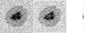 |
Fig. 1. Studied sunspot. Left: Original continuum map in 630 nm. The map size is 44 × 48 arcsec2. Middle: stray-light-corrected continuum map. White boxes show the different areas discussed later in the text. Right: negative of the kernel used to correct for the stray light. |
In addition to preparing the Stokes profiles with sp_prep.pro, we also corrected for the stray light using a telescope point spread function (PSF). Using PSF coefficients by Mathew et al. (2007) at 668.4 nm, which is close to the observed line spectra, we constructed a two-dimensional kernel. The kernel width is five steps (0.74 arcsec) or 5.0 times the pixel size equivalent to 2.5 times the spatial resolution. This is to avoid contamination by stray light and to prevent mixing the evolution of structures with each other (Beck et al. 2011). The kernel is shown in the right panel of Fig. 1.
To correct for the stray light using the kernel, we used the max_likelihood.pro routine. We evaluated variations of the quiet Sun standard deviation (contrast) as a function of iteration number. As shown in Fig. 2, the contrast increases at first but then levels off. Therefore, we used 15 iterations to avoid overcorrection and artifacts. The middle panel of Fig. 1 shows the corrected continuum map. The following analysis is based on stray-light-corrected data.
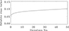 |
Fig. 2. Diagram of the rms of the normalized continuum intensity in the quiet Sun area around the sunspot versus iteration number. |
3. Results
3.1. Abnormal profiles
Following Ichimoto et al. (2007), we constructed single-wavelength Stokes V magnetograms away from the line center on far red and blue wings of both 630.15 and 630.25 nm lines. The magnetograms of the two lines were similar, and so we focused on the ±215 mÅ magnetograms of the first line.
Figure 3 displays the maps and histograms of those magnetograms. Histograms correspond to the entire field of view and are clearly asymmetric. The blue-wing magnetogram at −215 mÅ (left column in Fig. 3) has very few negative values in the penumbra (few negative values exist in the surrounding granulations). As the blue lobes of the Stokes V profiles of the main component are positive, any large value in the blue-wing magnetogram may suggest a hidden component with a large Doppler blueshift and the same polarity as the sunspot.
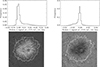 |
Fig. 3. Blue- and red-wing magnetograms. Upper row: histograms of Stokes V signals at wavelengths of −215 (left panel) and +215 mÅ (right panel) relative to the line core at 630.15 nm. Lower row: 2D images of Stokes V signals at the same wavelengths. The white contours show the boundary of the penumbra-quiet Sun. Histograms correspond to the entire region shown in the lower row. |
Pixels with a strong signal in the blue-wing magnetogram are spread all around the penumbra and have a grainy structure. These structures correspond to the penumbral filaments and upflow velocities (see the following section; Ichimoto et al. 2007, 2008). In contrast, in the red-wing magnetogram, there are both positive and negative values. The negative values are similar to those discussed above for the blue-wing magnetogram: they could be a manifestation of hidden components with the same polarity and a large redshift. We note that not every strong signal in the far-wing magnetograms corresponds to a hidden component, as a large magnetic field strength, turbulence, and temperature can broaden the lines. We therefore cannot specify an absolute threshold for the detection of the hidden components.
3.2. Abnormal profiles in selected areas
We selected five areas shown in Fig. 1 (C1 to C5) and studied the abnormal Stokes profiles along certain cuts. The Stokes profiles of the selected pixels along cuts C1 to C5 are shown in Figs. 4 to 8: profile arrays from left to right show the Stokes V profiles, the linear polarization profiles (LP =  ), and the Stokes I profiles. All Stokes profiles are normalized to their own continuum intensity. This normalization helps to visualize polarization signals better in darker areas. In the upper panels of Figs. 4 to 8, we show the maps of continuum intensity (left), and blue- and red-wing magnetograms (middle and right, respectively) for the selected areas. For improved visibility, we show the negative of the red-wing magnetogram. In these maps, the locations of the profiles shown in the lower panels are marked with black or white squares: profiles from bottom to top in the profile arrays correspond to the squares running from the umbra to the penumbra. In this study, we focus on newly identified abnormal Stokes V profiles showing a hump on both the blue and the red lobes of the Stokes V profiles with the same magnetic polarity as the spot (Hamedivafa 2023).
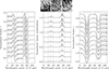 |
Fig. 4. Stokes profiles of selected pixels from area C1. The upper row displays 2D maps, which from left to right show continuum intensity, and blue- and red-wing magnetograms constructed from the first spectral line at −215 and +215 mÅ away from the line center, respectively. For ease of comparison, the negative of the red-wing magnetogram is shown. The same black or white curves are drawn to compare the locations of fine structures. The size of the selected area is 17 × 21 pixels, equivalent to 1.3 × 2.5 arcsec2. The lower row shows, from left to right, profile arrays of Stokes V, linear polarization (LP = |

3.2.1. Area C1
The cut C1 is along a penumbral filament in the inner penumbra, including a penumbral grain and a few peripheral umbral dots. As seen in the profile arrays of Fig. 4, locations co-spatial with umbral dots or penumbral grains show an extra hump on the blue lobe of the Stokes V profiles (referred to hereafter as an extra blue hump or simply a blue hump). The bright resolved granular structure in the blue-wing magnetogram (upper-middle panel) also corresponds to the bright points in the continuum map of the same area (upper-left panel). The leading edges of the penumbral filaments are seen as bright structures in both blue- and red-wing magnetograms.
Although the extra hump is seen clearly in the first line, there is often a broadening in the second line, perhaps due to a large Lánde gss factor of the second line (2.5 compared to 1.5; Nave et al. 1994). Generally, the hump is more clearly seen on the blue lobe than on the red lobe. An extra hump (red hump) can be seen on the red lobes of the Stokes V profiles for the outer part of the umbra. As we approach the bright penumbra, the red hump is no longer clearly visible. However, we find an enhancement in the far-red wing: we see a broadening in the red lobes, which means that the width of the red lobe has increased (see also Fig. 2 in Hamedivafa 2023). Upon inspection of the upper-right panel of Fig. 4 (the red-wing magnetogram), we see a pseudo-grainy structure similar to that seen in the blue-wing magnetogram but with less contrast. Also, we note that the bright structures in the two magnetograms (upper-middle and upper-right panels) are not necessarily co-spatial and there is no one-to-one counterpart for each bright structure (blue hump).
In the linear polarization profiles (Fig. 4, lower-middle panel), we see no significant effects of the presence of the extra hump component, although a slight asymmetry is evident in some profiles. Looking at the Stokes I profile array (lower-right panel), the asymmetry of the intensity profile, which manifests as stretching of the blue wing, is quite evident, especially in the first spectral line: there is noticeably greater line depth in the far-blue wing of the Stokes I profile.
3.2.2. Area C2
Similar to C1, this selected cut includes pixels on a set of aligned umbral dots resembling an intruding penumbral filament, penumbral grains, and the space between them (Fig. 5, upper-left panel). The blue hump or the stretching blue lobe of the Stokes V profile (lower-left panel) are obvious characteristics of the selected pixels. Comparing the bright grainy structure in the blue-wing magnetogram (upper-middle panel) with the continuum map of the same area (upper-left panel) indicates a phenomenological relation between the extra blue hump and penumbral grains or umbral dots, as seen in Fig. 4. Upon inspection of the Stokes V profiles belonging to the umbral dots (Fig. 5, the first three pixels running from the umbra) as well as the pixels in the diffuse background between penumbral grains (7th and 8th pixels), we clearly see the extra red hump or the stretching of the red lobe for both spectral lines. Concerning the rest of the selected pixels, the bright grains with smaller contrasts in the red-wing magnetogram (Fig. 5, upper-right panel) are noticeable effects of the non-visible red humps. Like C1, not all bright grains in the blue-wing magnetogram have bright counterparts in the red-wing magnetogram. Similar to what we see in C1, the linear polarization profiles show no significant signals corresponding to the extra hump component. The profiles of Stokes I also show an asymmetry due to the stretching of the blue wing.
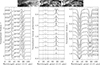 |
Fig. 5. Similar to Fig. 4 but for selected pixels from area C2. The size of the selected area is 53 × 9 pixels, which is equivalent to 7.9 × 1.4 arcsec2. Stokes profiles drawn from bottom to top correspond to the pixels running from umbra (left) to penumbra (right). The Stokes profiles in the panels showing profile arrays are sorted with a fixed step of 0.27, 0.18, and 0.25, from the left to the right panel, respectively. |
3.2.3. Area C3
This area shows a well-defined penumbral filament whose length covers almost the width of the penumbra. The selected pixels sample the penumbral grain and some pixels along the filament (Fig. 6). In all pixels, we clearly see the extra blue hump or the stretching of the blue lobe of the Stokes V profile, with locally strong signals (considering the Stokes V amplitude) in both spectral lines; see bottom-left panel. The blue-wing magnetogram (upper-middle panel) shows resolved bright grainy structures with different contrasts (similar to C1 and C2): the bright grains at the end of the filament have very little contrast and cannot be distinguished well, although the blue hump or the stretching of the blue lobe is well visible in the Stokes V profiles of the tail-end pixels. The asymmetry and partial stretching of the blue lobe of the linear polarization profiles for both spectral lines (lower-middle panel) can be seen in most of the pixels of this filament.
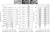 |
Fig. 6. Similar to Fig. 4 but for selected pixels from area C3. The size of the selected area is 28 × 10 pixels, which is equivalent to 4.2 × 1.6 arcsec2. Stokes profiles shown from bottom to top correspond to the pixels running from umbra (upper-right corner) to penumbra (lower-left corner). Stokes profiles in the panels of profile array are sorted with a fixed step of 0.2, 0.18, and 0.25 from the left to the right panel, respectively. |
In the red-wing magnetogram (Fig. 6, upper-right panel), bright structures are only seen around the penumbral grain with weak contrast, and are not observed along the filament. Also, there is no one-to-one co-spatial bright structure common to both the blue- and red-wing magnetograms. Due to the reduction in the amplitude of the Stokes V of the main component, and considering the signal of its linear polarization, we conclude that the magnetic field at the end of the filament is more horizontal relative to the local vertical, which is consistent with our general understanding of penumbral filaments (Keppens & Martínez Pillet 1996). There is also asymmetry in the Stokes I profiles (lower-right panel).
No red hump is seen along this penumbral filament, although Stokes V signals in the far-red wing for the first three pixels are not negligible. These significant signals cannot be due to the Doppler broadening in these pixels, because the first pixel that shows stronger Stokes V signals has lower continuum intensity (see the Stokes I profiles array in the lower-right panel). We find some other penumbral filaments with the same properties.
3.2.4. Area C4
This cut is selected inside the umbra so that its end reaches a penumbral grain (Fig. 7; see also Fig. 1). The extra blue and the red humps or the stretching of the blue and the red lobes of the Stokes V profiles can be seen in both spectral lines (lower-left panel of Fig. 7). This area is located in the umbra where the continuum intensity is weak and no umbral dot is clearly visible on the selected cut. However, grainy structures can be seen in the blue- and red-wing magnetograms (upper-middle and upper-right panels respectively), which correspond to the locally strong signals in both far wings. There are hidden Stokes V umbral dots that reveal themselves in these two magnetograms; these are perhaps related to the unresolved components that cause the extra humps.
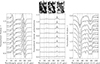 |
Fig. 7. Similar to Fig. 4 but for selected pixels from area C4. The size of the selected area is 8 × 18 pixels, which is equivalent to 1.2 × 2.9 arcsec2. Stokes profiles drawn from bottom to top correspond to the pixels running from umbra (lower-right corner) to penumbra (upper-left corner). The Stokes profiles in the panels showing the profile array are sorted with a fixed step of 0.2, 0.13, and 0.25 from the left to the right panel, respectively. |
3.2.5. Area C5
Similar to the area C4, the area C5 is selected inside the sunspot umbra but includes a set of umbral dots (Fig. 8). Stokes profiles of the selected pixels are shown in the lower panels; these sample a few umbral dots and the diffuse background between them. Bright grainy structures are seen in the blue- and red-wing magnetograms, (upper-middle and upper-right panels, respectively). This shows that the signals in these two far wings are stronger than those in the surrounding pixels.
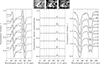 |
Fig. 8. Similar to Fig. 4 for area C5. The size of the whole selected area is 14 × 9 pixels, equivalent to 2.1 × 1.4 arcsec2. Stokes profiles drawn from bottom to top correspond to the pixels running from lower-left corner to upper-right corner. For a better comparison, the Stokes profiles in the panels of the lower row have been moved up with a fixed step of 0.25, 0.17, and 0.25, from the left to the right panel, respectively. |
Considering the first spectral line, the extra blue hump is more visible and recognizable than the extra red hump, although the far-red wing signals are stronger than or similar in strength to the far-blue wing signals. No noticeable signal is seen in the corresponding linear polarization profiles (Fig. 8, lower-middle panel). The asymmetry is still seen in Stokes I profiles. We found many other areas with similar properties to those discussed here.
3.3. Method of identifying abnormal Stokes V profiles
Here we focus on the identification of the Stokes V profiles whose unresolved components are seen as an extra hump on the red and/or blue lobes of the main component (as in the examples given in Figs. 4 to 8). The extra hump causes a bulge (or at least a change in curvature) in the far-red or blue lobe of the Stokes V profile. Therefore, by calculating the second derivative, we can examine the existence of a wavelength point in the far-red or blue lobe where the sign of the second derivative changes (hump position)1. Then, the profiles with an extra hump can be recognized. In this study, we examined the profiles of the pixels inside the penumbra and those of the outer part of the umbra; we note that the inner border of the studied area (extended penumbra) is defined as having a normalized intensity2 of greater than 0.35.
3.4. Statistics of the profiles with an extra hump
The histograms of the hump position are shown in Fig. 9. The hump position is defined as the wavelength point (relative to the zero-velocity reference) where the extra hump causes a change in the sign of the second derivative in the tail of the Stokes V lobes. If the hump positions were measured relative to the local Stokes V zero-crossing, we would obtain very similar graphs (not shown here).
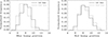 |
Fig. 9. Statistics of the hump positions. Left and right panels: Histogram of the blue and the red hump position, respectively (relative to the zero-velocity reference). Black and gray correspond to the first and the second lines, respectively. The units of the x-axis are spectral pixel of Hinode/SP (2.15 pm). See the main text for the definition of the hump position. |
About 50% (18%) of the pixels in the extended penumbra show at least an extra hump on the blue lobe of the first (second) spectral line (see the left panel of Fig. 9). This includes pixels that have only an extra blue hump and those with both a blue and a red hump. Similarly, 30% (14%) of the pixels show an extra hump on the red lobe of the first (second) spectral line (see the right panel of Fig. 9). The histogram peaks at a relative wavelength point between 7 and 9, that is, at a distance of 150 to 193 mÅ (equivalent to 7–9 km s−1) from the zero-velocity reference. The histograms are slightly skewed toward larger values.
Considering the first line, the histograms of the continuum intensity of the pixels showing only a blue (thin black) or a red (thin gray) hump are depicted in the left panel of Fig. 10. Also, the right panel of Fig. 10 shows the histograms of the continuum intensity of the pixels where the extra hump is seen on both lobes (thin black) and of the pixels where neither lobe of the Stokes V profile shows an extra hump (thin gray). There are fewer pixels that show this extra hump only in the red wing (9%) than pixels only showing a hump in the blue wing (29%). The corresponding graphs related to the second line are also similar to the graphs of the first line, and so we do not show these here.
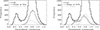 |
Fig. 10. Continuum intensity histogram of all penumbra pixels of the studied area. Left panel: histogram of the continuum intensity for pixels whose Stokes V profiles show only an extra blue (thin-black) or red (thin-gray) hump. Right panel: continuum intensity histogram of the pixels where the extra hump is seen on both the blue and the red lobe (thin-black), and the pixels where it is not seen on either lobe (thin-gray). For a better comparison, the vertical axis range is shortened from zero to 1000. |
By comparing the continuum intensity distributions in the left panel of Fig. 10, pixels that show only either the blue hump (29% in the first line and 15% in the second line) or the red hump (9% in the first line and 11% in the second line) seem to be located on the brighter parts of the penumbra (bright filaments or penumbral grains). The thin-black histogram in the right panel of Fig. 10, and especially the part of the histogram for the intensity range of 0.35–0.60, implies that pixels located in the darker parts of the penumbra (i.e., the inner penumbra, near to the umbra–penumbra border toward the umbra, as well as in the space between bright filaments) show the extra hump on both the blue and the red lobe. In contrast, there are bright pixels whose Stokes V profiles show both humps3 (right panel of Fig. 10: thin-black histogram for the intensities greater than 0.60, which show a shifted local peak toward lower intensities). A total of 21% in the first line and 3.0% in the second line show both a blue and a red hump. In addition, 21% (51%) of the pixels in the extended penumbra do not show any extra hump in the Stokes V profile of the first (second) line.
3.5. Examining possible correlations
The area and amplitude asymmetry of the Stokes V profiles are attributed to the existence of velocity gradients along the line of sight or perpendicular to this line in any spatial sampling (Auer & Heasley 1978). Due to the existence of unresolved components in each pixel, we examine the histograms of the amplitude asymmetry illustrated in Fig. 11 to investigate the effects of these components on the Stokes V amplitude. Amplitude asymmetry, δa, is calculated via Eq. (1) (Martínez Pillet et al. 1997):
 (1)
(1)
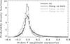 |
Fig. 11. Probability density function of Stokes V amplitude asymmetry corresponding to: all pixels of the penumbra (thick-black); to the pixels in which the extra hump is seen on both the blue and the red lobe of the Stokes V of the first line (thin-black); and to the pixels where the extra hump is seen on either the blue (thick-gray) or the red (thin-gray) lobe. |
where ab and ar are the blue and the red lobe amplitudes of the Stokes V profile, respectively.
Regardless of which lobe of the Stokes V profile of the main component displays the extra hump, the amplitude asymmetry distribution is the same and has a peak at zero (see Fig. 11). There are no large negative values in the amplitude asymmetries for the Stokes V profiles in which the extra hump is seen. No correlation is seen between the amplitude asymmetry and the either the maximum Stokes V signal at the hump position (hump amplitude) or the continuum intensity (see Fig. 12). However, the high-amplitude humps correspond to the low-amplitude asymmetries (upper panels of Fig. 12). The scatterplots of Stokes V amplitude asymmetry versus both hump position and distance between the blue and the red hump were also examined (not shown here), but no noticeable correlation was found.
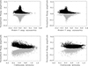 |
Fig. 12. Some scatter plots to investigate possible correlations. Upper row: scatter plots of normalized hump amplitudes versus Stokes V amplitude asymmetry for the first spectral line. Lower row: scatter plots of hump amplitude versus the corresponding continuum intensity. Left column: Plot for the pixels in which the extra hump is seen on both the blue (black circles) and the red (gray circles) lobe. Right column: Plot for the pixels where the extra hump is seen on either the blue (black circles) or the red (gray circles) lobe. |
A number of scatterplots considering the profiles showing both an extra blue hump and an extra red hump are illustrated in Fig. 13: the red and blue hump positions show no correlation with each other (upper-left panel), but the distance between them shows a strong correlation with either hump position, with a correlation coefficient of 0.80 (upper-middle and upper-right panels).
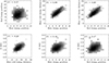 |
Fig. 13. Density plots for pixels showing the extra hump on both lobes. Here, the darker color indicates a higher density. Hump positions are measured from a zero-velocity reference. The correlation coefficients of the two quantities are marked on each panel. The magnetic field strength (lower row) was retrieved from the main component. |
The lower panels of Fig. 13 show a possible dependence of the hump position on the magnetic field strength of the main component: both the blue and the red hump position as well as the distance between the two humps are 0.46, 0.46, and 0.58 correlated with the magnetic field strength, respectively. The magnetic field strength is calculated by measuring the distance between the extremes of the blue and the red lobe of the main component of the Stokes V profile of the second spectral line, which is a Zeeman triplet. As seen in the upper-left panel of Fig. 13, there is no correlation between the blue and the red hump position: there is no evidence that one of the humps moves toward or away from the other, although their positions depend on the strength of the magnetic field (lower panels).
According to Fig. 14, the 2D image of the blue hump positions shows a simple order in the extended penumbra: larger values of this quantity with a higher population density are located in the inner penumbra (toward the umbra), although large and small values are scattered all over the penumbra. The similar 2D images for the red hump position and blue-red hump distance show similar order in the penumbra (not shown here). This order, as seen in the graphs of the lower panels of Fig. 13, can be related to the radial variations of magnetic field strength in the penumbra.
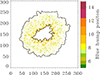 |
Fig. 14. Two-dimensional maps of blue hump position. The map was constructed using profiles that show an extra hump on both the blue and the red lobe of the Stokes V profile. Other pixels can be seen as the background with white color in the image. The black contours show the defined inner and outer boundaries of the enumbra. |
For a quantitative investigation of the finding that these quantities are larger in the inner penumbra (even inside the umbra) than those in the outer penumbra, the relation of the blue and the red hump positions as well as of the blue-red hump distance versus radius are shown in Fig. 15. We define the radius as the distance from the geometric center of the sunspot. The averages of these three quantities are calculated in the rings with a certain width drawn in the left panel of Fig. 15. The error bars show the standard deviation of each quantity in the corresponding rings. The right panel of Fig. 15 confirms this finding.
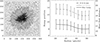 |
Fig. 15. Radial variations of the blue and the red hump positions and of the blue-red hump distance. Left panel: continuum intensity map. Right panel: distance of the red and the blue humps (gray and black solid lines, respectively) from a zero-velocity reference for the first spectral line as well as the distance between them (dashed line) versus the geometric distance from the sunspot center (radius). Each data point in the right panel illustrates the average of the quantities in the defined white rings in the left panel. Error bars show the standard deviation of each quantity in each ring. |
Considering the profiles that show a hump on both the blue and the red lobe, we also examined the radial variations of hump amplitude (normalized to its local continuum intensity) and Stokes V amplitude asymmetry. The results are shown in Fig. 16. On average, the normalized hump amplitude at the umbra and inner penumbra, where we measure a larger magnetic field strength, is higher than that in the outer penumbra (solid lines). We then separated the positive and negative amplitude asymmetries; the absolute value of amplitude asymmetry, on average, increases with radius (dashed lines).
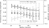 |
Fig. 16. Radial variations of normalized hump amplitude (solid lines) and Stokes V amplitude asymmetry (dashed lines). Each data point illustrates the average of the quantities in the defined white rings in the left panel of Fig. 15. Error bars show the standard deviation of each quantity in each ring. |
4. Discussion
Full Stokes profiles of a mature sunspot close to the disk center were obtained using the Hinode Solar Optical Telescope SP. In a continuation of the work by Hamedivafa (2023), we present a systematic study to detect hidden magnetic component(s) by checking for the existence of extra humps in the far wings of Stokes V profiles in the defined (extended) penumbra, and investigate their statistical properties. Also, we study the correlation of the blue and the red humps (detected on the blue and the red lobes, respectively) and find their radial variation from the sunspot center.
Franz & Schlichenmaier (2009) found evidence of profiles of opposite polarity within the penumbra using Hinode data. Katsukawa & Jurčák (2010) also presented a few examples of one extra hump in Stokes V found for a delta spot close to the disk center. An extra hump in the blue lobe of Stokes V was previously observed by Bellot Rubio et al. (1999) in the quiet Sun area and was discussed by Steiner (2000). Franz & Schlichenmaier (2013), using Hinode/SP data, studied three-lobed Stokes V profiles to find traces of magnetic fields of opposite polarity in the outer penumbra.
We find traces of both positive and negative humps in the red-wing magnetograms (see Fig. 3). Like positive humps in the blue wing, a negative hump in the red wing can be the tracer of a hidden magnetic field. Jurčák & Katsukawa (2010) suggested another interpretation for the negative humps in the red wing. These authors synthesized similar profiles using a one-component photospheric model with a suitable stratification for the line-of-sight velocity set to 2.5 km s−1 below log(τ) = 0.3.
Pixels with positive signals in the red-wing magnetogram (white pixels in the lower-right panel of Fig. 3) are supposed to have opposite polarities and large Doppler shifts. These opposite-polarity pixels are located in the middle to outer penumbra and on the penumbra-quiet Sun border. These large positive signals of Stokes V in the red wing are attributed to downflows of the Evershed flows along magnetic field lines returning into the photosphere at the penumbral boundary (Westendorp Plaza et al. 2001; Bellot Rubio et al. 2004; Ichimoto et al. 2007; Shimizu et al. 2008) or to the sea-serpent field lines in the mid-penumbra as proposed by Sainz Dalda & Bellot Rubio (2008).
Franz et al. (2016) studied the topology of the penumbral magnetic field and searched for the opposite-polarity profiles (either reversed polarity or three-lobed profiles). These authors found that the number of three-lobed profiles in the infrared 1565 nm lines is much lower than those in the visible 630 nm lines. Similarly to Schlichenmaier & Collados (2002) and to Franz & Schlichenmaier (2013), Franz et al. (2016) presented a model atmosphere that harbors a jump in the line-of-sight velocity and magnetic field strength. They discussed a scenario to reproduce the three-lobed profiles: a configuration of strong plasma flow and opposite-polarity magnetic field.
Comparing the present work with the papers mentioned above, we discard reversed polarity and three-lobed Stokes V profiles and focus on extra humps rather than lobes. We employ an identification method based on the second derivative of the Stokes V profiles to extract weak extra humps in the wings. In addition, the relation or statistics of the blue and the red humps was not studied in the mentioned works. We note that the humps we discuss here show a similar magnetic polarity to the main component, while extra lobes (three-lobed profiles) are usually due to an opposite magnetic polarity.
Many profiles show an extra hump on the tail of the blue and/or red lobes of the main component of the spectral lines at 630.15 and 630.25 nm (Figs. 4 to 8). The extra hump is more clearly visible in the 630.15 nm line (the first line) than in the 630.25 nm line (the second line). For both spectral lines, the extra hump is more frequently observed in the blue lobe than in the red lobe. However, at the umbra–penumbra border, as well as inside the umbra, the extra humps are more frequently detected on both blue and red lobes simultaneously. If one does not account for the extra humps, the overall effect is an additional broadening of the line profile. This can be interpreted as a large micro-turbulence or higher temperature in Stokes inversions.
We also measured the continuum intensity, magnetic field strength, and Stokes V asymmetry of the main component along with the amplitude and wavelength position of the extra humps. Although we find a positive correlation between the hump position and the magnetic field strength of the main component (Fig. 13, lower panels), there is no significant correlation between the hump amplitude and either the continuum intensity or the amplitude asymmetry of the main component. We also find that large normalized hump amplitudes are co-spatial to the locations with small Stokes V asymmetry (inside the umbra and at the umbra–penumbra border; see Figs. 12 and 16).
We find evidence for modification of the Doppler shifts and amplitudes of the humps by strong Stokes V signals. We averaged the values in elliptical rings within the umbra and penumbra (Figs. 15 and 16). The distance between the blue and the red hump slightly decreases and then levels off with radial distance from the sunspot center (dashed line in Fig. 15); in other words, it shows a modest modification, while the vertical magnetic field of the penumbra decreases by around one kiloGauss from the middle to the outer penumbra. This is also seen in the graph of the hump positions (solid lines in Fig. 15). This presumably confirms the effect of strong Stokes V signals on the humps: in cases of limited Zeeman splitting in the outer penumbra, the position and amplitude of the humps remain intact. As can be seen in Fig. 16, in contrast to the amplitude asymmetries (dashed lines), the normalized amplitudes of both the blue and the red hump (solid lines) decrease with radial distance.
Although it clearly appears that the distance between the blue and the red hump correlates with each hump position, the blue and the red hump position are independent (upper panels of Fig. 13). If these two extra humps were the result of a single Doppler-shifted unresolved component (the first scenario), they would move together and we would expect the wavelength positions of the two humps to show a negative correlation. In other words, as the two humps have the same relative Doppler shift with respect to the main component one expects to find a negative correlation between their positions. Such a correlation is not observed.
There is another explanation for the first scenario that some of our findings may support. Assuming that the unresolved magnetic component is just a very broad single (blueshifted) absorption line with a moderate Doppler velocity (up to 3 km s−1), the red lobe of its Stokes V is not far from the red lobe of the main component (causing the lack or weakness of its visibility; we note that the red hump is not detected well). Nevertheless, the positive blue lobe of the main component shows a positive hump of the unresolved component. The expected large width of this unresolved absorption line requires a magnetic field strength of greater than 3000 Gauss. However, the hump amplitudes as well as the signals in the far wings of Stokes linear polarization are weak (see the lower-middle panels of Figs. 4 to 8). If the second component were to have a small filling factor, this could explain the weak Stokes signals of the two humps. Nevertheless, as described above, a single component does not explain the absence of a correlation between the positions of the two humps. In other words, there is evidence that the two humps are independent. Therefore, not all of our findings are in favor of a single unresolved component as the origin of the simultaneous appearance of the extra blue and red hump.
The signals of the linear Stokes profiles co-spatial with the extra humps are very small. To explain this, in addition to the small size of the filling factor of the magnetic field responsible for the humps, there are two other possibilities. Either the transverse magnetic field is weak or there are entangled transverse magnetic field lines with significant cancelation. It is known that the Zeeman Stokes signals suffer significant cancelation in unresolved structures. However, this is not a reasonable explanation for the weak linear polarization signals in the umbra.
The existence of both positive and negative extra humps on the blue and red lobes of Stokes V can be explained with the assumption of two hidden magnetic components (the second scenario) with the same polarization as the sunspot, and large Doppler velocities (about 6 km s−1 or smaller, inferred from the histograms shown in Fig. 9). Therefore, according to the interpretation of the second scenario, inward plasma flows with high velocities are coupled to large outward plasma flows. Both these two unresolved magnetic components occur at the same time and in their vicinity. The quenching of the inward plasma flow by the dense plasma of the photosphere could also be the reason for the lack of visibility of the extra hump in the far-red wing (Rezaei et al. 2007) in some pixels.
According to the uncombed penumbra model, there are two magnetic structures in the penumbra: one is more horizontal and channeled in the filaments, while the other is rather close to vertical (Solanki & Montavon 1993). While the Evershed flow follows the filamentary structure of the penumbra, the background vertical magnetic field in the penumbra emerges from between bright filaments. This background component was one of the candidate drivers of the chromospheric jets in the penumbra observed in the Ca II H filtergrams of the Hinode/SOT (Katsukawa et al. 2007). It is speculated that the interaction of the background fields with the magnetic flow in filaments can result in magnetic reconnection, which can produce far-wing humps (Katsukawa & Jurčák 2010).
5. Summary
To search for traces of hidden magnetic components in sunspots, we analyzed the Stokes profiles of the neutral iron lines at 630 nm within a round sunspot close to the disk center in NOAA 10944. In the extended penumbra, including the outer part of the umbra, we obtained the following findings4: (1) 59% of the pixels clearly show at least an extra hump in the far wings of the Stokes V profile of the 630.15 nm line, indicating a hidden magnetic component. Especially in the penumbra, the existence of at least one unresolved component with the same polarity as the sunspot seems to be common. This unresolved component has an outward Doppler velocity in many pixels or an inward Doppler velocity in some cases.
(2) Around 21% of the Stokes V profiles of the 630.15 nm line show an extra hump in each of the two lobes simultaneously. The distance between the two humps as a function of radius levels off in the umbra, decreases in the penumbra, and then levels off to a lower value toward the quiet Sun border. Investigating the continuum intensity distribution of the profiles with two humps suggests that many of those are co-spatial with dark penumbral filaments or belong to the umbra with a pseudo-grainy structure (Stokes V umbral dots).
We discuss two possible scenarios to explain Stokes V profiles that show both a blue and a red hump: (a) The first is the existence of a single unresolved component that is considerably broadened (Zeeman saturation) and has a Doppler velocity of up to 3 km s−1. This unresolved component is associated with a large magnetic field (of the order of 3000 Gauss). However, the independence of the blue and the red hump position does not support this scenario. (b) The second involves the presence of two unresolved components with probably small filling factors and large Doppler velocities (about 6 km s−1 or smaller): one upward (creating the blue hump) and the other downward (creating the red hump). These unresolved components have a pseudo-grainy spatial distribution in the photosphere of both umbra and penumbra. The humps seen on both the red and blue wings of Stokes V profiles inside umbra can also be explained as two unresolved components. However, a component with a weak and quasi-vertical magnetic field and a high velocity in the vicinity of the stationary main component of the umbra with a large and vertical magnetic field cannot be explained at the present time.
A significant linear polarization signal was only detected for a small fraction of all humps. Therefore, we refrain from speculating about the magnetic inclination of the hump component(s). The present findings suggest there may be a relationship between the formation mechanism of umbral dots and the bright structures in the sunspot penumbra with unresolved component(s); the nature of this relationship remains to be determined. A study of the temporal evolution of the extra hump position and its amplitude could also bring us closer to understanding the origin of the extra humps.
For instance, we assume that the blue lobe is positive. Then, moving from the maximum of the lobe towards its tail, the second derivative changes sign: it is initially negative and then becomes positive. If the second derivative becomes negative once more, this indicates the presence of a blue hump.
The intensity map was smoothed using a suitable boxcar.
Many Stokes V profiles in the umbra have the same features, but have a main component with a smaller absolute amplitude, which is due to the low intensity of the umbra.
Our identification procedure ignored about 20% of the Stokes V profiles, including the reversed-polarity and three-lobed profiles as well as profiles with very small amplitude or width.
Acknowledgments
We would like to thank the anonymous referee for valuable and constructive comments on the manuscript. Data analysis was, in part, carried out on the Multi-wavelength Data Analysis System (MDAS) operated by the Astronomy Data Center (ADC), National Astronomical Observatory of Japan (NAOJ). Hashem Hamedivafa sincerely thanks Yukio Katsukawa for his supports for MDAS account. Hinode is a Japanese mission developed and launched by ISAS/JAXA, with NAOJ as domestic partner and NASA and UKSA as international partners. It is operated by these agencies in cooperation with ESA and NSC (Norway).
References
- Auer, L. H., & Heasley, J. N. 1978, A&A, 64, 67 [NASA ADS] [Google Scholar]
- Beck, C., Rezaei, R., & Fabian, D. 2011, A&A, 535, 129 [Google Scholar]
- Bellot Rubio, L. R., Ruiz Cobo, B., & Collados, M. 1999, A&A, 341, L31 [NASA ADS] [Google Scholar]
- Bellot Rubio, L. R., Balthasar, H., & Collados, M. 2004, A&A, 427, 319 [NASA ADS] [CrossRef] [EDP Sciences] [Google Scholar]
- Borrero, J. M., & Ichimoto, K. 2011, Liv. Rev. Sol. Phys., 8, 4 [Google Scholar]
- Franz, M., & Schlichenmaier, R. 2009, A&A, 508, 1453 [NASA ADS] [CrossRef] [EDP Sciences] [Google Scholar]
- Franz, M., & Schlichenmaier, R. 2013, A&A, 550, A97 [EDP Sciences] [Google Scholar]
- Franz, M., Collados, M., Bethge, C., Schlichenmaier, R., Borrero, J. M., et al. 2016, A&A, 596, A4 [Google Scholar]
- Hamedivafa, H. 2023, Iran. J. Astorn. Astrophys., 10, 139 [Google Scholar]
- Ichimoto, K., Shine, R. A., Lites, B. W., et al. 2007, PASJ, 59, 593 [Google Scholar]
- Ichimoto, K., Tsuneta, S., Suematsu, Y., et al. 2008, A&A, 481, L9 [NASA ADS] [CrossRef] [EDP Sciences] [Google Scholar]
- Jurčák, J., & Katsukawa, Y. 2010, A&A, 524, 21 [Google Scholar]
- Katsukawa, Y., & Jurčák, J. 2010, A&A, 524, 20 [Google Scholar]
- Katsukawa, Y., Berger, T. E., Ichimoto, K., et al. 2007, Science, 318, 1594 [NASA ADS] [CrossRef] [Google Scholar]
- Keppens, R., & Martínez Pillet, V. 1996, A&A, 316, 229 [Google Scholar]
- Martínez Pillet, V., Lites, B. W., & Skumanich, A. 1997, ApJ, 474, 810 [CrossRef] [Google Scholar]
- Mathew, S. K., Martínez Pillet, V., Solanki, S. K., & Krivova, N. A. 2007, A&A, 465, 291 [NASA ADS] [CrossRef] [EDP Sciences] [Google Scholar]
- Nave, G., Johansson, S., Learner, R. C., Thorne, A. P., & Brault, J. W. 1994, ApJS, 94, 221 [NASA ADS] [CrossRef] [Google Scholar]
- Rempel, M., & Schlichenmaier, R. 2011, Liv. Rev. Sol. Phys., 8, 3 [Google Scholar]
- Rezaei, R., Schlichenmaier, R., Schmidt, W., & Steiner, O. 2007, A&A, 469, L9 [NASA ADS] [CrossRef] [EDP Sciences] [Google Scholar]
- Sainz Dalda, A., & Bellot Rubio, L. R. 2008, A&A, 481, L21 [NASA ADS] [CrossRef] [EDP Sciences] [Google Scholar]
- Sánchez Almeida, J., & Lites, B. W. 1992, ApJ, 398, 359 [CrossRef] [Google Scholar]
- Scharmer, G. B. 2009, Space Sci. Rev., 144, 229 [NASA ADS] [CrossRef] [Google Scholar]
- Scharmer, G. B., & Spruit, H. C. 2006, A&A, 460, 605 [NASA ADS] [CrossRef] [EDP Sciences] [Google Scholar]
- Schlichenmaier, R., & Collados, M. 2002, A&A, 381, 668 [NASA ADS] [CrossRef] [EDP Sciences] [Google Scholar]
- Schlichenmaier, R., Jahn, K., & Schmidt, H. U. 1998, ApJ, 493, L121 [NASA ADS] [CrossRef] [Google Scholar]
- Shimizu, T., Lites, B. W., Katsukawa, Y., et al. 2008, ApJ, 680, 1467 [NASA ADS] [CrossRef] [Google Scholar]
- Sigwarth, M. 2001, ApJ, 563, 1031 [NASA ADS] [CrossRef] [Google Scholar]
- Solanki, S. K. 2003, A&ARv, 11, 153 [Google Scholar]
- Solanki, S. K., & Montavon, C. A. P. 1993, A&A, 275, 283 [NASA ADS] [Google Scholar]
- Steiner, O. 2000, Sol. Phys., 196, 245 [NASA ADS] [CrossRef] [Google Scholar]
- Suematsu, Y., Tsuneta, S., Ichimoto, K., et al. 2008, Sol. Phys., 249, 197 [Google Scholar]
- Thomas, J. H., & Weiss, N. O. 2004, ARA&A, 42, 517 [Google Scholar]
- Tsuneta, S., Ichimoto, K., Katsukawa, Y., et al. 2008, Sol. Phys., 249, 167 [Google Scholar]
- Westendorp Plaza, C., del Toro Iniesta, J. C., Ruiz Cobo, B., & Martínez Pillet, V. 2001, ApJ, 547, 1148 [NASA ADS] [CrossRef] [Google Scholar]
All Figures
|
Fig. 1. Studied sunspot. Left: Original continuum map in 630 nm. The map size is 44 × 48 arcsec2. Middle: stray-light-corrected continuum map. White boxes show the different areas discussed later in the text. Right: negative of the kernel used to correct for the stray light. |
| In the text | |
|
Fig. 2. Diagram of the rms of the normalized continuum intensity in the quiet Sun area around the sunspot versus iteration number. |
| In the text | |
|
Fig. 3. Blue- and red-wing magnetograms. Upper row: histograms of Stokes V signals at wavelengths of −215 (left panel) and +215 mÅ (right panel) relative to the line core at 630.15 nm. Lower row: 2D images of Stokes V signals at the same wavelengths. The white contours show the boundary of the penumbra-quiet Sun. Histograms correspond to the entire region shown in the lower row. |
| In the text | |
|
Fig. 4. Stokes profiles of selected pixels from area C1. The upper row displays 2D maps, which from left to right show continuum intensity, and blue- and red-wing magnetograms constructed from the first spectral line at −215 and +215 mÅ away from the line center, respectively. For ease of comparison, the negative of the red-wing magnetogram is shown. The same black or white curves are drawn to compare the locations of fine structures. The size of the selected area is 17 × 21 pixels, equivalent to 1.3 × 2.5 arcsec2. The lower row shows, from left to right, profile arrays of Stokes V, linear polarization (LP = |
| In the text | |
|
Fig. 5. Similar to Fig. 4 but for selected pixels from area C2. The size of the selected area is 53 × 9 pixels, which is equivalent to 7.9 × 1.4 arcsec2. Stokes profiles drawn from bottom to top correspond to the pixels running from umbra (left) to penumbra (right). The Stokes profiles in the panels showing profile arrays are sorted with a fixed step of 0.27, 0.18, and 0.25, from the left to the right panel, respectively. |
| In the text | |
|
Fig. 6. Similar to Fig. 4 but for selected pixels from area C3. The size of the selected area is 28 × 10 pixels, which is equivalent to 4.2 × 1.6 arcsec2. Stokes profiles shown from bottom to top correspond to the pixels running from umbra (upper-right corner) to penumbra (lower-left corner). Stokes profiles in the panels of profile array are sorted with a fixed step of 0.2, 0.18, and 0.25 from the left to the right panel, respectively. |
| In the text | |
|
Fig. 7. Similar to Fig. 4 but for selected pixels from area C4. The size of the selected area is 8 × 18 pixels, which is equivalent to 1.2 × 2.9 arcsec2. Stokes profiles drawn from bottom to top correspond to the pixels running from umbra (lower-right corner) to penumbra (upper-left corner). The Stokes profiles in the panels showing the profile array are sorted with a fixed step of 0.2, 0.13, and 0.25 from the left to the right panel, respectively. |
| In the text | |
|
Fig. 8. Similar to Fig. 4 for area C5. The size of the whole selected area is 14 × 9 pixels, equivalent to 2.1 × 1.4 arcsec2. Stokes profiles drawn from bottom to top correspond to the pixels running from lower-left corner to upper-right corner. For a better comparison, the Stokes profiles in the panels of the lower row have been moved up with a fixed step of 0.25, 0.17, and 0.25, from the left to the right panel, respectively. |
| In the text | |
|
Fig. 9. Statistics of the hump positions. Left and right panels: Histogram of the blue and the red hump position, respectively (relative to the zero-velocity reference). Black and gray correspond to the first and the second lines, respectively. The units of the x-axis are spectral pixel of Hinode/SP (2.15 pm). See the main text for the definition of the hump position. |
| In the text | |
|
Fig. 10. Continuum intensity histogram of all penumbra pixels of the studied area. Left panel: histogram of the continuum intensity for pixels whose Stokes V profiles show only an extra blue (thin-black) or red (thin-gray) hump. Right panel: continuum intensity histogram of the pixels where the extra hump is seen on both the blue and the red lobe (thin-black), and the pixels where it is not seen on either lobe (thin-gray). For a better comparison, the vertical axis range is shortened from zero to 1000. |
| In the text | |
|
Fig. 11. Probability density function of Stokes V amplitude asymmetry corresponding to: all pixels of the penumbra (thick-black); to the pixels in which the extra hump is seen on both the blue and the red lobe of the Stokes V of the first line (thin-black); and to the pixels where the extra hump is seen on either the blue (thick-gray) or the red (thin-gray) lobe. |
| In the text | |
|
Fig. 12. Some scatter plots to investigate possible correlations. Upper row: scatter plots of normalized hump amplitudes versus Stokes V amplitude asymmetry for the first spectral line. Lower row: scatter plots of hump amplitude versus the corresponding continuum intensity. Left column: Plot for the pixels in which the extra hump is seen on both the blue (black circles) and the red (gray circles) lobe. Right column: Plot for the pixels where the extra hump is seen on either the blue (black circles) or the red (gray circles) lobe. |
| In the text | |
|
Fig. 13. Density plots for pixels showing the extra hump on both lobes. Here, the darker color indicates a higher density. Hump positions are measured from a zero-velocity reference. The correlation coefficients of the two quantities are marked on each panel. The magnetic field strength (lower row) was retrieved from the main component. |
| In the text | |
|
Fig. 14. Two-dimensional maps of blue hump position. The map was constructed using profiles that show an extra hump on both the blue and the red lobe of the Stokes V profile. Other pixels can be seen as the background with white color in the image. The black contours show the defined inner and outer boundaries of the enumbra. |
| In the text | |
|
Fig. 15. Radial variations of the blue and the red hump positions and of the blue-red hump distance. Left panel: continuum intensity map. Right panel: distance of the red and the blue humps (gray and black solid lines, respectively) from a zero-velocity reference for the first spectral line as well as the distance between them (dashed line) versus the geometric distance from the sunspot center (radius). Each data point in the right panel illustrates the average of the quantities in the defined white rings in the left panel. Error bars show the standard deviation of each quantity in each ring. |
| In the text | |
|
Fig. 16. Radial variations of normalized hump amplitude (solid lines) and Stokes V amplitude asymmetry (dashed lines). Each data point illustrates the average of the quantities in the defined white rings in the left panel of Fig. 15. Error bars show the standard deviation of each quantity in each ring. |
| In the text | |
Current usage metrics show cumulative count of Article Views (full-text article views including HTML views, PDF and ePub downloads, according to the available data) and Abstracts Views on Vision4Press platform.
Data correspond to usage on the plateform after 2015. The current usage metrics is available 48-96 hours after online publication and is updated daily on week days.
Initial download of the metrics may take a while.