| Issue |
A&A
Volume 691, November 2024
|
|
|---|---|---|
| Article Number | A170 | |
| Number of page(s) | 22 | |
| Section | Stellar structure and evolution | |
| DOI | https://doi.org/10.1051/0004-6361/202450607 | |
| Published online | 11 November 2024 | |
High-resolution spectroscopy of detached eclipsing binaries during total eclipses
1
Nicolaus Copernicus Astronomical Center, Polish Academy of Sciences, ul. Rabiańska 8, 87-100 Toruń, Poland
2
Astronomical Observatory Institute, Faculty of Physics, Adam Mickiewicz University, ul. Słoneczna 36, 60-286 Poznań, Poland
3
Faculty of Physics, University of Warsaw, ul. Pasteura 5, 02-093 Warsaw, Poland
⋆ Corresponding author; This email address is being protected from spambots. You need JavaScript enabled to view it.
Received:
3
May
2024
Accepted:
28
September
2024
Abstract
Context. We present results of high-resolution spectroscopic observations of detached eclipsing binaries (DEBs) with total eclipses, for which UVES spectra were obtained during the phase of totality. These observations serve as a key way to determine the age and initial metallicity of the systems and to verify evolutionary phases of their components and distances.
Aims. With the additional, independent information concerning the effective temperature and metallicity of one of the components, we aim to estimate the precise ages of the studied binaries and show the usefulness of totality spectra. The second goal was to provide precise orbital and physical stellar parameters of the components of systems in question.
Methods. Using the VLT/UVES, we obtained high-resolution spectra of 11 DEBs during their total-eclipse phase. Atmospheric parameters of then-visible (larger) components were obtained with iSpec. With additional spectroscopy from the Comprehensive Research with Échelles on the Most interesting Eclipsing binaries (CRÉME) project, public archives, and literature, we obtained radial-velocity (RV) measurements, from which orbital parameters were calculated. Photometric time-series observations from TESS and ASAS were modelled with the JKTEBOP code, and, combined with RV-based results, they allowed us to obtain physical parameters for nine double-lined systems from our sample. All the available data were used to constrain the ages with our own approach, utilising MESA isochrones. Reddening-free, isochrone-based distances were also estimated and confronted with Gaia Data Release 3 (GDR3) results.
Results. We show that single spectroscopic observations taken during a total eclipse can break the age-metallicity degeneracy and allow for the precise determination of the age of a DEB. With high-quality spectroscopic and photometric data, we are able to reach a 5−10% level of uncertainty (e.g. 724−24+52 Myr). Even for single-lined DEBs, where absolute masses are not possible to obtain, the spectroscopic analysis of one of the components allows one to put strong constraints on the properties of both stars. For some cases, we noted inconsistencies between isochrone-based and GDR3 distances. For one binary, which could not be fitted with a single isochrone (RZ Eri), we suggest a new explanation.
Key words: stars: atmospheres / binaries: eclipsing / stars: fundamental parameters
© The Authors 2024
 Open Access article, published by EDP Sciences, under the terms of the Creative Commons Attribution License (https://creativecommons.org/licenses/by/4.0), which permits unrestricted use, distribution, and reproduction in any medium, provided the original work is properly cited.
This article is published in open access under the Subscribe to Open model. This email address is being protected from spambots. You need JavaScript enabled to view it. to support open access publication.
1. Introduction
Detached eclipsing binaries (DEBs), especially those that are also double-lined spectroscopic binaries (SB2s), are one of the most important sources of direct determination of stellar parameters (Torres et al. 2010). The precision and accuracy of direct (and absolute) mass and radius measurements is unrivalled thanks to the advent of high-stability spectrographs and satellite-borne photometric observations. Stellar parameters of hundreds of well-studied DEBs, from our Galaxy and the Magellanic Clouds (Southworth 2015; Eker et al. 2014; Graczyk et al. 2014), constitute the foundation of a number of astrophysical studies (such as stellar formation and evolution) testing the performance of satellite observations, the characterisation of exoplanet hosts, or the cosmic distance scale. Stars with high-quality measurements, spanning a vast range of various stellar parameters such as masses, spectral types, metallicities, or evolutionary stages, are used as benchmark stars; that is, calibrators to validate analysis methods, cross-calibrate surveys, or improve data products of a survey (Blanco-Cuaresma et al. 2014a; Maxted 2023).
The assessment of precise and accurate effective temperatures (Teff) and metallicities ([M/H]) in DEBs (and SB2s in general) from spectroscopic observations is actually more complicated than in the case of single stars. The light that is instantaneously recorded comes from two sources, which can be very different from each other. One can be treated as a contamination of the other. For this reason, for many DEBs, which are otherwise well studied, we lack information about metallicity, and the temperatures of their components are calculated from colour indices (if multi-band photometry is available) and colour-temperature relations. For systems studied in the XX century, the relations in question are now obsolete, but no modern attempts have been made to revisit those systems. Additionally, without [M/H] it is difficult to assess the age of a system, due to the age-metallicity degeneration. For example, on the main sequence (MS), a more metal-rich star is older than a metal-poor star of the same mass and Teff; on the red giant branch (RGB), isochrone fitting can give an error of ∼20 Myr for a fixed metallicity, while the error increases to ∼300 Myr when a ±0.1 dex uncertainty in [M/H] is introduced, and so on. It is thus clear that for modern stellar astrophysics, knowledge of [M/H] is necessary.
A special class of DEBs, which allow for an easier determination of a number of stellar characteristics, are the totally eclipsing pairs. Geometry requires components of a totally eclipsing DEB to clearly differ in radii, which means either different evolutionary phases (e.g. RG+MS) or significantly unequal masses. Depending on the system, the totality phase can last from less than an hour to several days (not taking into account some extreme and exotic scenarios). During the totality, light of only one star is observed, which is not being ‘contaminated’ by the companion; thus, any observations taken at that time are in fact of a single star. This allows us to, for example, apply simpler analysis techniques, appropriate for single stars; simplify light-curve modelling, as some of the degeneracies (e.g. inclination vs. sum of the radii) are less important; or directly obtain the flux ratio and observed colour indices (when multi-band photometry is available) of the components.
The concept of dedicated observation in total eclipses is not new, but it is rarely presented; this is probably because of the difficulties in planning the observations, which arise from demanding time constraints. Some examples include studies of late-type components of exotic eclipsing systems such as post-common-envelope binaries GH Vir (Fulbright et al. 1993) and NN Ser (Haefner et al. 2004) and a ζAur-type star 31 Cyg (Bauer & Bennett 2014). Other cases include the larger giants in double-RG eclipsing binaries HD 187669 (Hełminiak et al. 2015) and ASAS J061016−3321.3 (Ratajczak et al. 2021). More recently, it was discovered that totally eclipsing DEBs are excellent benchmark objects for the upcoming PLAnetary Transits and Oscillations of stars (PLATO; Rauer et al. 2014) mission, and programmes aimed at in-eclipse spectroscopic observations have been initiated (P. Maxted, priv. comm.).
In this publication we present the results of this kind of a dedicated programme, which served as a proof of concept. Its main goal was to show how much our knowledge of a given binary system can be improved with just a single spectrum taken with proper timing. The paper is structured as follows: in Sect. 2, we present the studied targets; Sect. 3 describes the observations of the main project, as well as supplementary data; the methodology is described in Sect. 4, followed by the results and notes for specific systems; Sect. 5 contains a discussion of the results; concluding remarks are given in Sect. 6.
2. Target selection
This work is a sub-project of a larger undertaking named Comprehensive Research with Échelles on the Most interesting Eclipsing binaries (CRÉME; Hełminiak et al. 2022). The main spectrographs used by this project are: CHIRON at the SMARTS 1.5-m telescope in CTIO (Chile), HIDES at the OAO-188 telescope in Okayama (Japan), CORALIE at the 1.2-m Euler telescope in La Silla (Chile), and FEROS at the MPG-2.2 m telescope, also in La Silla. Substantial contributions were made with the HARPS (ESO-3.6 m, La Silla) and HRS (SALT, South Africa) instruments, and minor contributions with other facilities, including HDS and IRCS (Subaru, Maunakea), SOPHIE (OHP, France), FIES (NOT, La Palma), or HARPS-N (TNG, La Palma).
The targets for CRÉME were primarily selected from the All-Sky Automated Survey (ASAS) Catalogue of Variable Stars (ACVS; Pojmanski 2002). We selected relatively bright (V < 12 mag) DEBs, which are suitable for high-resolution spectroscopic observations and have the colour index V − K > 1.1 mag, suggesting spectral types F and later, with abundant spectral features. For the purpose of this particular study, we searched for total eclipses by visually inspecting the available ASAS-3 light curves. In some cases, the ephemerides had to be refined, since the value of the orbital period (P) given directly in the ACVS did not produce a satisfactory-looking phase-folded light curve. Once the acceptable values of P and zero-phase (T0) were obtained, we estimated the length of the flat part of a total eclipse (Δϕtot). We used a conservative approach of under-estimating Δϕtot in order to compensate for uncertainties in P and T0. Simultaneously, with ongoing CRÉME observations, we also ruled out a number of triple systems, where the third light could contaminate the spectrum taken in totality.
The ACVS targets were supplemented with a number of objects known from the literature to show total eclipses, for which estimating Δϕtot was possible. We note, however, that this literature search was incomplete. In total, we identified ∼40 objects, mainly from the Southern hemisphere, 11 of which were observed in a dedicated programme with the Ultraviolet and Visual Echelle Spectrograph (UVES; Dekker et al. 2000) and are reported in this work. In eight cases, the primary (deeper) eclipse is the total one, suggesting a cooler, inflated secondary (sub-giant or giant) that is more evolved than the primary. In the remaining three cases, the smaller and cooler secondary hides completely behind the hotter and larger primary, strongly suggesting that both components are main-sequence (MS) stars. A few other notable examples, with totality spectra obtained from non-dedicated CRÉME observations, have already been published; for example, HD 187669 (Hełminiak et al. 2015) or ASAS J061016−3321.3 (Ratajczak et al. 2021).
3. Data
3.1. UVES Spectroscopy in total eclipses
Since the spectroscopic observations in totalities have to be taken in a specific, short time window, we wanted to employ a queue-based instrument installed at a large-aperture telescope, operated in a service mode. We chose the UVES spectrograph, mounted at the VLT UT2 telescope, located at the ESO’s Cerro Paranal observatory (Chile). Our observations were made using only the Red arm, cross-disperser #3, and slicer #1. This setting gave us the wavelength range of 4779–6808 Å, with a gap from 5765–5828 Å. The slit width was set to 0.7 arcsec, which resulted in spectral resolving power of ∼57 000. The observations took place during semester P93, between April and September 2014. Observing windows were calculated on the basis of the ephemeris and light-curve morphology known at the time, and incorporated as timing constraints in the observing blocks (OBs) submitted to the observatory. Table 1 summarises the UVES observations, together with positions and distances from Gaia Data Release 3 (GDR3; Gaia Collaboration 2016, 2023).
Basic information about targets and log of the UVES observations made during total eclipses.
Spectra were reduced with the pipeline provided by ESO, and the reduced products were downloaded from the ESO archive. For the analysis, we used the 1D-merged, wavelength-calibrated, and barycentric-corrected spectra.
3.2. Supplementary spectroscopy
Apart from spectra taken in total eclipses, we also report spectroscopic observations used for radial-velocity (RV) determination and binary modelling. The majority of the studied systems were included in the CRÉME sample, but also into other researchers’ projects (e.g. Graczyk et al. 2021), whose primary goals were different from those of this work but related to the derivation of stellar parameters.
The supplementary spectroscopic observations, used for systems from this study, are briefly described in Table 2. We note that the publication by Ratajczak et al. (2016) on BQ Aqr was in fact based on the CRÉME data. It includes one CHIRON spectrum taken in totality, but the signal-to-noise ratio (S/N) was too low for a proper spectral analysis. For the remaining two systems – RZ Eri and SZ Cen – we relied on the literature data. The former was recently observed by Merle et al. (2024), whose RV measurements we used in this work. We combined them with earlier data from Popper (1988) to obtain a very long time baseline. The latter dataset was used in previous analyses of RZ Eri (Burki et al. 1992; Vivekananda Rao et al. 1994). The most up-to-date RV data for SZ Cen are from Andersen (1975), and they were also used in the study by Gronbech et al. (1977).
Observing log of supplementary CRÉME and archival ESO spectroscopy.
3.3. Supplementary photometry
Most of our systems had not been studied before, and no dedicated photometry was collected. For those already known from the literature, the observations either come from small-aperture, all-sky surveys (ASAS, SuperWASP), or they were taken decades ago. As a follow-up of the CRÉME project, we systematically applied for the short-cadence photometry through the Guest Investigator (GI) programmes of the Transiting Exoplanet Survey Satellite (TESS; Ricker et al. 2014). Those observations are summarised in Table 3.
TESS photometry of studied systems used in this work.
To date, ten of our systems have space-borne photometric observations available, although SZ Cen in long cadence only (we used QLP photometry from sectors 11 and 38, taken with 1800 and 600 seconds of cadence, respectively). In two cases – A141235 and A180413 – the orbital period is much longer than the time spent by the satellite in a single sector; thus, no eclipses have been recorded for A141235 so far, and only one primary (no secondary) has been recorded for A180413. One of our systems – A161710 – was not in the field of view of TESS at all, although it might be during Cycle 7. We applied for GI observations of this target, as well as those of A180413.
The available light curves (LC) are used for binary modelling. Together with RVs, they allow us to obtain absolute values of key stellar parameters, including masses M and radii R, and thus the gravitational acceleration log g, which can also be estimated directly from the spectra. Additionally, for short-period, tidally locked systems (orbital period Porb is the same as the rotational Prot), we can also estimate the projected rotational velocity v sin i, which is also retrievable from the spectra. Values of log g and v sin i from the binary modelling can thus be used as a reference for spectral analysis. In summary, for eight systems we were able to base our reference log(g) and v sin i estimates on the TESS data, and for four we were only able to use the ASAS and ASAS-SN photometry.
4. Analysis and results
Below we describe the procedures used in this study, with the focus being on the analysis of the UVES spectra and application of its results. The binary RV+LC modelling approach, although necessary for this publication, is the same as in previous CRÉME-based studies and is here described only briefly. The detailed descriptions of the implemented methodology can be found in previous publications that are based on CRÉME data (see e.g. Ratajczak et al. 2016, 2021; Hełminiak et al. 2017, 2021; Kahraman Aliçavuş et al. 2023; Moharana et al. 2023, and references therein).
4.1. New and updated eclipsing binary models
The RVs were measured with our own implementation of the TODCOR routine (Zucker & Mazeh 1994), with synthetic template spectra, and individual measurement errors calculated with a bootstrap procedure (Hełminiak et al. 2012). The RV solutions were found using the V2FIT procedure (Konacki et al. 2010), which was used to fit a single- or double-Keplerian orbit to a set of RV measurements of one or two components, utilising the Levenberg-Marquardt minimisation scheme.
To model the light curves, we used version 40 (v40) of the JKTEBOP code (Southworth et al. 2004), which is based on the EBOP program (Popper & Etzel 1981). The out-of-eclipse variations (likely coming from activity) and long-term brightness trends were modelled simultaneously with stellar parameters with the aid of 5th degree polynomials and sine functions, as described in Hełminiak et al. (2021). For long-cadence data of SZ Cen, we used the option of numerically integrating over a specified exposure time interval (120 s here). Parameter errors were estimated with a Monte Carlo procedure implemented in JKTEBOP (Task 8).
The above scheme was used for all systems except RZ Eri. We typically use V2FIT and JKTEBOP separately, as the former allows for fitting additional parameters, such as differences between zero points of two spectrographs, perturbations of the systemic velocity of a binary (linear, quadratic, periodic), or non-Keplerian effects (for more details see Konacki et al. 2010). For RZ Eri, we decided to fit all the data (LC+RV) simultaneously within JKTEBOP. The reason was that the solution of Popper (1988) has an assumed orbital period, given without uncertainties, which does not correspond to the TESS light curve; that is, the time between two secondary eclipses (in S05 and S32) was not an integer multiple of the assumed P. The TESS curve alone does not have enough information to accurately estimate the P and orbital eccentricity e, as it only covers one primary and two secondary eclipses. By adding the new RV data from Merle et al. (2024) we obtained a time base long enough to overcome those obstacles. A reliable orbital+LC solution could only be obtained by fitting all datasets simultaneously.
The resulting RV and LC solutions are shown in Figs. A.1 and A.2, respectively. The key orbital, stellar, and physical parameters from the RV+LC analysis are shown in Table A.1. Since A141235 and A180413 are single-lined spectroscopic binaries (SB1), absolute values of their stellar parameters were not possible to determine. For previously studied targets, comparison of our results with literature is presented in Table A.2.
4.2. Analysis of spectra in totality
For the sake of clarity, we henceforth use the following naming convention. The component that is visible during the totality, and whose spectra were recorded with UVES, is the ‘spectroscopic’ one, and the other is referred to as the ‘companion’. Their respective parameters are indexed as ‘spec’ and ‘comp’, respectively. The spectroscopic component is obviously larger and more massive (evolved), but it is not always the hotter one.
For the determination of atmospheric parameters, we used v20230804 of the Python code iSpec (Blanco-Cuaresma et al. 2014b; Blanco-Cuaresma 2019)1. Before the analysis, the UVES spectra were first continuum normalised with SUPPNet (Różański et al. 2022)2. Then, radial velocities were calculated using the iSpec module that utilises a cross-correlation function; and they were later used to shift the spectra, so their RVs were equal to zero. We also recalculated the flux errors on the basis of the S/N (see Table 1). In this way, we made sure the resulting uncertainties are trustworthy, which was verified by the reduced χ2 given in the output.
We applied the spectral synthesis method, mostly utilising the code SPECTRUM (Gray & Corbally 1994), the Model Atmospheres with a Radiative and Convective Scheme (MARCS) grid of model atmospheres (Gustafsson et al. 2008), and solar abundances from Grevesse et al. (2007). Results were being verified with other choices of those settings, and adopted only if results were consistent. The iSpec synthesises spectra in certain user-defined ranges called ‘segments’. We followed the default approach, where these segments are defined as regions ±2.5 Å around a certain line. We decided to synthesise spectra around a set of lines carefully selected in such way that various spectral fitting codes reproduce consistent parameters from a reference solar spectrum (Blanco-Cuaresma et al. 2016).
In general, we run fits with the following parameters set free: the effective temperature (Teff), logarithm of gravity (log(g)), metallicity ([M/H]), α-element enhancement ([α/Fe]), microturbulence (vmic), and projected rotational velocities (vsin(i)). The spectral resolution R was set fixed to the instrument’s value of ∼57 000, the limb darkening coefficient was set to 0.6, and the radial velocity was set to zero. The macroturbulence velocity vmac, which degenerates with rotation, was at all times calculated on the fly by iSpec from an empirical relation. It is valid only for Teff < 6600 K, and above that value we set vmac to zero.
From the RV+LC models described in previous section, we obtained the reference values of log(g) for the spectroscopic components, which we were able to directly compare to the values found with iSpec. We noted a typical situation where the precision and accuracy of the spectroscopy-based results are worse than for the ‘dynamical’ log(g) from the RV+LC approach. Due the small dynamical log(g) errors, the iSpec-based values were often outside of the ±3σ range, and overall agreement was rather poor (occurring mainly thanks to large iSpec uncertainties). Therefore, for nearly all SB2 systems – except AL Ari – we decided to repeat the spectral analysis with log(g) fixed to the RV+LC values. This situation naturally caused concerns about the quality of the results for the SB1 systems. Unfortunately, we are not able to verify them other than by checking the consistency of the results through, for example, a comparison with isochrones and distance (see the next section).
Results of the iSpec fits are presented in Table 4. Figure 1 shows the observed UVES spectra with synthetic ones, created in iSpec on the basis of the resulting parameters. Table A.2 shows a comparison between various results from this work, including the iSpec analysis, and the literature.
Atmospheric parameters of ‘spectroscopic’ components of the studied systems, obtained from iSpec analysis of the UVES spectra.
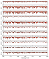 |
Fig. 1. Fragments of spectra of studied objects: observed, taken during total eclipses (black), and synthetic (red) created with iSpec from parameters listed in Table 4. All spectra are corrected for the barycentric and radial velocities and normalised to the continuum. They are plotted in the same scale to emphasise differences between them. |
Two of the stars we studied had had their components analysed spectroscopically before. AL Ari was presented in Graczyk et al. (2021), where decomposed spectra of both components were analysed with the code GSSP (Tkachenko 2015). The set of fitted parameters was very similar to ours, with the only difference being that the vmac was set free, and the [α/Fe] was not taken into account. The overall agreement is very good in all parameters, except for vmac itself, which they found to be much smaller (5.8 ± 2.0 km/s) than our value taken from an empirical relation (9.83 km/s). The reason most likely is that the effective temperature (6540 K) is close to the range of applicability of the relation. In other aspects, such as the results of the RV+LC analysis (Table A.2), our results are also in very good agreement with Graczyk et al. (2021).
Deconvolved spectra of individual components of BQ Aqr were analysed by Ratajczak et al. (2016) with the code SME (Valenti & Piskunov 1996). In that work, only the Teff and total metallicity [M/H] were fitted, while log(g) and vsin(i) were held fixed to the values found in their RV+LC analysis (synchronised rotation was assumed). The Teff of the larger star found by Ratajczak et al. (2016) – 4490 ± 230 K – is in reasonable agreement with ours (4630 ± 100 K), although mainly thanks to large uncertainties. The agreement in metallicity is weaker, at the level of 2.6σ: +0.12 ± 0.11 from SME versus −0.25 ± 0.09 from iSpec. However, Ratajczak et al. (2016) calculated the overall [M/H] without [α/Fe] with SME, while from iSpec we obtained [M/H] and [α/Fe]. In the case of BQ Aqr we found a substantial enhancements of α elements, which can partially explain the disagreement between our results and Ratajczak’s. Most of the other stellar parameters, such as the absolute radii or log(g), are similar for both works (see Table A.2), with the exception of Teff, comp (≡Teff, 1).
4.3. Age determination
We estimate the ages of our systems using a simple procedure called ISOFITTER, which operates by comparing the results with isochrones produced using a dedicated web interface3, based on the Modules for Experiments in Stellar Astrophysics (MESA; Paxton et al. 2011, 2013, 2015, 2018) and developed as part of the MESA Isochrones and Stellar Tracks project (MIST v1.2; Choi et al. 2016; Dotter 2016). We generated a grid that covers ages 107.0 to 1010.2 Gyr in logarithmic scale every log(τ) = 0.01. For each age we generated isochrones for metallicities between −4.0 dex to +0.5 dex, with variable step: 0.05 above −0.5 dex and 0.1 below that value. Additionally, we did not include post-AGB phases.
Each isochrone is composed of so-called equivalent evolutionary points (EEPs), taken from evolutionary tracks for a given initial mass. Primary EEPs are a series of points that can be identified in all stellar-evolution tracks (Dotter 2016), including the zero-age main sequence (ZAMS), tip of the red giant branch (RGBTip), and so on. The secondary EEPs (EEPs henceforth) are chosen to equally split each phase on an evolutionary track into smaller segments. A single EEP can list various information about a model of a star, but the most important for us are age log(τ), initial mass Minit, current stellar mass M, initial metallicity [Fe/H]init, current metallicity [Fe/H], effective temperature log(Teff), gravity log(g) (which we translate to radius R), luminosity log(L), and synthetic absolute magnitudes in different bands (we were interested in Johnson-Cousins U, B, V, RC, IC, 2MASS J, H, K, and TESS). We highlight the distinction between the initial and current values of mass and metallicity, which over time may differ significantly. This is due to stellar winds and atomic diffusion, respectively (Choi et al. 2016; Dotter et al. 2017). EEPs with the same age are combined in an isochrone by the MIST web interface.
We now introduce the nomenclature we used. With ISOFITTER we searched for the best-fitting model of a given binary, which means a pair of EEPs of the same age and initial metallicity (i.e. laying on the best-fitting isochrone) that best reproduce a number of observed and measured stellar properties. We also define accepted isochrones as those that contain models that meet the assumed criteria; these typically predict values at most 3σ from the measured or observed value. In some cases, we also forced other constraints, such as the more evolved component being more massive, or the larger (spectroscopic) component being strictly cooler or hotter than the companion, depending on the depths of eclipses. We note that in our approach the best-fitting isochrone contains the best-fitting model, but it may also contain some accepted models.
The goodness of fit of each accepted model was evaluated by a χ2-like parameter, which is calculated as
 (1)
(1)
where x0, i is the value of parameter x predicted by the given model, xi is the observed or measured value of this parameter, σi is its uncertainty, and the summation is done over all the parameters that are constraining the fit. The model with the lowest χ2 was considered to be the best. It is important to note that we did not make any interpolation between single isochrones of different ages and metallicities, nor between EEPs within one isochrone. Our fits are based purely on a pre-defined grid.
The uncertainties were also calculated in a simplified way. The most optimal approach in isochrone fitting for single stars would be to use the Bayesian formalism, as, for example, in Pont & Eyer (2004). In our case, it would be quite complicated, because we fit to data for two stars, and for each component we have different measurements (i.e. no spectroscopic data for the companion). We also use constraints based on relative parameters (ratio of fluxes or radii), or observables embedded in a non-trivial way (observed magnitudes in the distance calculation; see the rest of the text). We thus base our uncertainty estimates on the accepted models; that is, the distribution of the searched parameters among models that meet the fitting criteria. As explained in Pont & Eyer (2004), if the uncertainties of observations or measurements are much smaller than the scale over which the prior of the observed or measured quantity varies, the probability distribution of the prior can be neglected, and a Bayesian approach does not need to be applied. We believe that this is fulfilled in most, if not all, of our cases; thus, the non-Bayesian formalism may be applied. Additionally, since our fits are based purely on a pre-defined grid, steps of the grid are included in the uncertainties.
The set of parameters used as constraints in fits varies between the SB2 and SB1 systems. In general, for SB2s we used results of the RV+LC analysis: M and R of both components and lcomp/lspec flux ratio in the LC band; distance to the system from Gaia and results of the iSpec analysis; Teff and [Fe/H] (current) of the spectroscopic component. For the SB1 systems, instead of RV+LC results, we were only able to use LC-based results, namely the fractional radii of each component r (≡R/a, where a is the major semi-axis of the binary’s orbit) and the flux ratio. We did, however, add the spectroscopic log(g) value from iSpec. To calculate a, which is necessary for estimating r, we took two stellar masses (from two EEPs), the orbital period P, and eccentricity e from the RV or LC analysis, and applied Kepler’s third law. The isochrone-predicted values of flux ratios can be obtained from difference of absolute magnitudes of two EEPs:
 (2)
(2)
The isochrone-predicted, reddening-free distance diso was estimated simultaneously with the reddening E(B − V), using the available observed total magnitudes in different filters, and the predicted total brightness of the system in the same filters for a given pair of EEPs. Distances in each available band dλ were calculated from Teff–surface brightness relations from Kervella et al. (2004). Then, they were transformed to distance moduli (m − M)λ with the standard relation (m − M) = 5log(d)−5. Due to the interstellar extinction and reddening, individual values of (m − M)λ ≡ (m − M)0 + Aλ were obviously not in agreement. To obtain the extinction-free modulus (m − M)0, we fitted a straight line on the kλ vs (m − M)λ plane, where the kλ = RV(Aλ/AV) are extinction coefficients in each band. We followed the extinction law of Cardelli et al. (1989)AU : AB : AV : AR : AI : AJ : AH : AK = 4.855 : 4.064 : 3.100 : 2.545 : 1.801 : 0.880 : 0.558 : 0.360, which assumes RV = 3.1. The slope of the fitted line in this approach is the reddening E(B − V), while the intercept is the extinction-free modulus (m − M)0, which can be translated into the distance d0:
 (3)
(3)
A graphical explanation is shown in Fig. 2, in a case where five bands were used: B, V, J, H, and K (without U, R, and I).
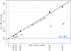 |
Fig. 2. Graphical explanation of distance and reddening determination method. The distance moduli (m − M)λ, calculated from observed magnitudes and synthetic photometry in different bands, are plotted (black dots) as a function of their corresponding law coefficient, by which we define the applied extinction law. The slope and the intercept of the fitted line (solid black) are the values of E(B − V) and reddening-free distance modulus (m − M)0, respectively. The (m − M)0 level is shown in blue. Differences between (m − M)0 and each (m − M)λ represent extinction values Aλ in each band (in mag), and they are also labelled. |
The results of ISOFITTER runs, with all available parameters (with few exceptions that will be described later), are summarised in Table 5. For each target, we show values of the best-fitting model of the following parameters: age (in Gyr), initial metallicity (in dex), effective temperature of the unseen companion (in K), and isochrone-predicted distance (in pc). For each of those, we also list uncertainties, which are defined as a range of values taken from accepted isochrones corresponding to the 16th-to-84th percentile of the parameter’s distribution. Additionally, for the two SB1 systems we report the masses and radii of their components. For A141235, we obtained  M⊙,
M⊙,  R⊙ for the spectroscopic component and
  M⊙,
M⊙,  R⊙ for the companion. Analogously, for A180413 we obtained
  M⊙,
M⊙,  R⊙, and
  M⊙,
M⊙,  R⊙.
R⊙.
Results of isochrone fitting.
We also want to stress that the [Fe/H]init of the best-fitting model does not have to coincide with the value found in iSpec, for several reasons. First, we used a grid in [Fe/H]init without interpolation. Second, in MESA/MIST isochrones and tracks, metallicity of a star changes in time, often by more than 0.10 dex. One such example is AL Ari, for which the resulting [Fe/H]init = −0.15, while the current value for the spectroscopic component [Fe/H] = −0.32, as given in the best-fitting model. Finally, the value determined from spectra has its own uncertainty; thus, a range of metallicities should be used in isochrone fitting, which is not always the case in the literature.
The scheme above has been applied to all our systems, with the exception of RZ Eri. It has been suggested several times in the literature that this binary has undergone a major event, namely a significant mass loss from the evolved component that vastly disturbed its evolution. Therefore, assuming an independent evolution, coevality, and fitting a single isochrone to both components is meaningless. In the case of RZ Eri, we run ISOFITTER twice to look for the age of each component separately. Obviously, we only use masses, radii, and metallicity (from iSpec), as well as Teff in one case. No comparison with the GDR3 distance has been made.
In Figs. 3–5, we show the best-fitting isochrones with our results on various parameter spaces: M − R, M − Teff, lcomp/lspec − R, and lcomp/lspec − Teff for SB2s (for RZ Eri only the first two), and Teff − log(g) and lcomp/lspec − Rcomp/Rspec for SB1s. The age and metallicity of the isochrone and the distance the model predicts are also given. Errors of our results are shown as ±1σ or 16th-to-84th percentile. For some SB2 systems, one of the parameters was not used in the fitting process (see the next section), and its values, given by the accepted models, are shown in the figures as grey dots.
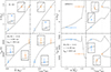 |
Fig. 3. Comparison of parameters of SB2 systems with isochrone (black line) containing best-fitting model (open square symbols for two components). Age and initial metallicity for the isochrone are given, together with the predicted distance. Measurements and indirect determinations of stellar parameters are marked with filled dots with error bars, and their associated models are marked with open squares. Components labelled ‘spectroscopic’ are represented with orange symbols, while the ‘companions’ are shown with light blue ones. For each object, we show M − R, lcomp/lspec − R, M − Teff, and lcomp/lspec − Teff panels. On the lcomp/lspec panels, the isochrones were scaled with respect to the absolute magnitude of the model that matches the ‘spectroscopic’ component; thus, it is by definition located on the grey dashed line that marks the unity. In cases where a certain parameter was not used as a constraint in the fitting process (e.g. Rcomp for AL Ari or lcomp/lspec for SZ Cen), its model values from all the accepted isochrones are shown with grey dots. Zoomed-in images of the vicinity of the determined parameters were drawn for clarity in the insets. Here, we show results for AL Ari and A084011, while other systems are presented in Fig. A.3. |
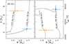 |
Fig. 4. Isochrones fitted to the components of RZ Eri separately, shown only on the M − R (left) and M − Teff (right) planes. The isochrones are labelled with their age (in gigayears) and initial metallicity. Colour-coding for the components is the same as in Figs. 3 and A.3. |
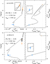 |
Fig. 5. Same as Figs. 3 and A.3, but for SB1 systems (top: A141235; bottom: A180413) and on different planes. We only show Teff − log(g) (left) and lcomp/lspec − Rcomp/Rspec (right). On the latter, the spectroscopic component is shown without errors, and set by definition to (1.0;1.0). Flux ratios refer to the ASAS V band. |
5. Discussion
The main goal of this work is to compare the process of isochrone fitting and age determination in cases where additional spectroscopic information is given with the situation in which it is not (i.e. results from RV+LC only). We did not aim to obtain precise and accurate stellar ages. This would require the use of several stellar evolution models, and adding some systematic effects into the uncertainty budget. In particular, a number of our systems contain active sub-giant and giant stars and belong to the RS CVn variability class. Activity and possible enhanced mass loss (due to stellar winds for instance; Eggleton & Yakut 2017) may not be sufficiently implemented into the models we used. Additionally, they may not be well fitted to binary systems if the binarity affected evolution of one of the components. This might be one of the reasons behind the difficulties in fitting a single isochrone to our measurements or discrepancies with Gaia distances, which we encountered for several systems (A084011, BQ Aqr). However, since the same models and measurements were used for cases with and without spectroscopic information, the comparison of those two cases should be reliable and free of major systematics. Being aware of the above, we now discuss our results.
5.1. Ages and metallicities with and without spectroscopy
To directly show the usefulness of having independent estimates of metallicity and effective temperatures, for example from spectra taken in totality, for each system (with the exception of RZ Eri) we ran isochrone fits in two cases: without and with results from the iSpec analysis. In both cases, distance was also taken into account. Results are shown in Fig. 6, on a [Fe/H]init versus log(τ) plane.
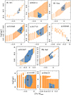 |
Fig. 6. Graphical presentation of age-metallicity degeneration in isochrone fitting of the studied systems on the [Fe/H]init vs. log(τ) planes. Orange symbols represent the accepted isochrones in fits constrained only by the RV+LC (for SB2s) or LC-based (for SB1s) parameters. Blue points are accepted isochrones after including spectroscopy in the set of constraints. The white stars mark the isochrones that contain the best-fitting models. Significant reduction in allowed ages and initial metallicities is clearly seen in almost all cases, even when spectroscopic parameters were not well constrained. The SB2 systems are shown on the top three rows (without RZ Eri), while the two SB1 systems are shown in the lowest one. |
Isochrones, for which models were found to be in a 3σ agreement with measured stellar masses, radii (if SB2), fractional radii (if SB1), and flux ratio only, are shown in orange. The blue points represent isochrones that contain models with an additional 3σ agreement with the metallicity and effective temperature of the larger component, plus its log(g) for SB1s, as determined from UVES spectra. One can see, especially for SB2s, that the orange points form bands, showing strong degeneracy between the age and metallicity. This means that having only the masses, radii, and ratios of fluxes is not sufficient for a meaningful age determination, even though l2/l1 is very well determined in systems with total eclipses. The addition of distance often helps to rule out some extreme values, but it does not solve the degeneracy completely. With information about only one component, the Teff, [Fe/H] (note, it may be different for each star), and log(g) (if unknown before), we can narrow down the range of possible ages, even if the errors in atmospheric parameters are relatively large (e.g. A191947). It can be compared to reducing something of the size of a bottle of wine to the size of its label. Cases such as A084011, SZ Cen, or A161710 show that not only [Fe/H], but also the temperature, help to solve the degeneracy, as there are isochrones for acceptable metallicities that do not meet other criteria.
The improvement in age determination is shown more qualitatively in Fig. 7. We compare ages found with the use of Teff, spec and [Fe/H]spec (X-axis) with those found based on RV+LC parameters (and distance) only (Y-axis). The three ‘youngest’ points are our two SB1 systems (A141235 shown twice, see text). The ages themselves are generally in good agreement (left panel). The central panel directly compares uncertainties from both approaches, where we plot ranges of the age distribution of accepted isochrones corresponding to their 16th-to-84th percentile (±1σ for normal distribution). It shows that if the spectroscopic data are used, age is always better determined. The most striking example is the SB1 system A180413, with 0.44 dex reduced to 0.13 dex in log(τ). The best SB2 example is A084011, with the 0.20 dex uncertainty reduced to 0.05.
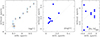 |
Fig. 7. Determination of stellar age through isochrone fitting for cases with and without spectroscopic constraints. The grey dotted line on each panel shows the equality relation (y = x). Left: Logarithm of age (log(τ)). Uncertainties from each approach are shown with different colours for easier comparison. Centre: Uncertainties in age Δlog(τ) defined as 16th-to-84th percentile or ±1σ ranges. Right: Comparison of best-fitting initial metallicities [Fe/H]init. |
We note that similar behaviour can also be seen for most of the other parameters, such as Teff, spec, Teff, comp, and others not taken into account in the fit (i.e. Rcomp for AL Ari). The best fits with and without spectroscopy are mostly similar, but with significantly smaller errors in the former. This also applies to Teff, spec determined from iSpec and purely from isochrone fit.
The exception to this rule is initial metallicity, which can be seen in the right panel of Fig. 7. The results without spectroscopy can be very different from those obtained with it. If they agree, it is most likely coincidental. Two stars of the same mass and different metallicities should have different effective temperatures, luminosities, and hence absolute magnitudes. Thus, in principle, the distance to a star (or a binary in our case) could help to indirectly constrain the Teff and [Fe/H]. In general, we do see such behaviour in our results, but even with constraints on d, the [Fe/H]init is not very well determined (typically with ±0.2−0.4 dex uncertainty).
A141235 is an interesting case, as without spectroscopic constraints we found two solutions of equal χ2: for ([Fe/H]init, log(τ)) = (−0.7, 8.36) and (+0.1, 8.31). Between these two, one can find many models with only a slightly worse fit quality. This is of course due to very loose constraints coming from the quality of the photometric data (ASAS) and the fact that the GDR3 distance was not taken into account. Despite that, the age seems to be determined with good precision; however, it is still under-estimated (log(τ) = 8.53 from the full fit).
5.2. Totality versus disentangled spectra
The aim of this work was to show the usefulness of spectra taken during total eclipses (through dedicated and carefully programmed observations) in studies of eclipsing binaries, in particular in determining the age by obtaining an independent estimate of temperature and metallicity of one of the components. This is obviously limited to the totally eclipsing systems. There are, of course, other means of achieving the same goal from a set of individual spectra of any SB2 (not only totally eclipsing), taken in different orbital phases, when lines of both stars are seen. If the fluxes of both stars are roughly comparable, both components can thus be successfully analysed. For example, the GSSP code (Tkachenko 2015) includes a ‘composite’ mode, where atmospheric parameters of both components are found simultaneously from a single observed spectrum. The most popular approach, however, is the separation of individual components from a number of composite spectra through some sort of a disentangling technique (a.k.a. deconvolution, decomposition; e.g. Bagnuolo & Gies 1991; Simon & Sturm 1994; Hadrava 1995; Ilijic et al. 2004; Konacki et al. 2010; Tkachenko et al. 2022).
In several cases where both disentangled and totality spectra were used (Hełminiak et al. 2015; Ratajczak et al. 2021), the resulting atmospheric parameters are in a very good agreement. The disentangled spectra typically have higher S/Ns, because they are constructed of a number of single observations – the more composite spectra, the higher the S/N of the deconvolved ones. Another advantage of disentangling is the ease and flexibility of planning the observations. The spectra can be taken at almost any time during the orbital period, as long as they cover different orbital phases and RV values of the components, and there is a sufficiently large number of them. With high S/N of the individual spectra (> 70), one can sometimes obtain satisfactory deconvolution after as few as five-to-six visits (Hełminiak et al. 2021; Miller et al. 2022), although some methods require minimum of eight (Konacki et al. 2010).
On the contrary, planning the observations for totality is difficult because of the short time frame. For some short-period systems, the window of opportunity only lasts a couple of hours4; although, it opens up many times per observing season, every orbital period. It may, however, be challenging to have the telescope ready for the precise moment or to gather a sufficient S/N in a relatively short time. For long-period binaries, the totality can last up to a few days, but it only appears every couple of months or less often. It is easy to imagine the loss of such an opportunity due to weather or technical problems. It was most likely for these planning and time-constraining reasons that our original programme was not carried out completely on UVES.
The huge advantage comes, however, with the telescope time – a single visit during the eclipse is enough, while disentangling requires multiple observations, but with a sufficient S/N (we want to note that for meaningful RV measurements, an S/N of ∼20−30 is often enough, while spectra that will undergo disentangling should optimally have S/N > 50). The further data analysis is also simpler, as the disentangling is itself a complicated process prone to systematic errors (e.g. from incorrect continuum normalisation) that further affect the results. Disentangling is mathematically an under-determined problem, meaning that there are more variables than data, and various results can reproduce the given input. The products are thus affected by systematic trends, which need to be carefully corrected for (Ilijic et al. 2004). Then, the decomposed spectra need to be re-scaled based on the flux contribution from each component or the flux ratio, which itself is wavelength dependent and does not have to coincide with the flux ratio obtained from the LC fit. Improper re-scaling will lead to incorrect depths of spectral lines.
A quick solution to this is to take a spectrum during the total eclipse with the same instrument and settings. The line profiles and depths are thus known for one of the components, which makes the whole spectral decomposition process much easier and faster. Totality spectra can thus effectively support and simplify the deconvolution.
In summary, we can conclude that even on its own, without other spectroscopic observations or without a full RV+LC model of the binary, a totality spectrum provides valuable information about the spectroscopic component, and the system as a whole. The optimal observational strategy for comprehensive studies of totally eclipsing DEBs, which is balanced between minimal telescope resources and maximal scientific output, could thus be as follows:
-
Obtain one totality spectrum with high S/N (≳80).
-
Obtain a few (4−6) out-of-eclipse spectra with the same instrument and somewhat lower S/N (∼40−60) for disentangling.
-
Obtain many more (> 10) observations with even lower S/N (∼20−30), possibly with smaller telescopes and lower resolution spectrographs, for RV measurements.
6. Conclusions
In this paper, we present 11 totally eclipsing DEBs, which we modelled with available spectroscopic and photometric data and which were observed with VLT/UVES during their total eclipses. The UVES observations allowed for direct and independent characterisation of one of the components, which we call ‘spectroscopic’, and putting strong constraints on the nature of the second component (‘companion’) and the system as a whole. The majority of our targets did not have, until now, their ages or their stellar and orbital parameters determined.
We find that with good spectral analysis results for at least one star of a binary, one can significantly lower the uncertainty in age estimation, assess the initial metallicity of the whole system, and even point out stellar parameters with problematic or uncertain results, such as Gaia DR3 distances or radii of inflated components. Most of our age determinations have precision levers better than 10%, even down to 5% for the best case. We also conclude that without spectroscopic constraints the metallicity cannot be securely estimated with isochrones, even with high-precision distance and quality RV+LC analysis.
Some observatories, offering queue or service mode observations, do not accept programs with short windows.
In case of eccentric orbits the tidal spin-orbit equilibrium occurs for stellar rotation periods different than Porb.
Acknowledgments
We would like to thank the anonymous Referee for invaluable comments and suggestions. We would like to thank the staff of the observatories involved in this work, especially the VLT/UVES, for conducting the challenging, yet successful observations. KGH would like to thank Dr. Pierre Maxted from the School of Chemical and Physical Sciences of the Keele University, and Dr. Nikki Miller from the Nicolaus Copernicus Astronomical Center of the Polish Academy of Sciences (NCAC PAS), who independently picked up a similar idea, for discussions on the topic. We would also like to thank Dr. Tomasz Kamiński, Thomas Steinmetz, and Ayush Moharana (all from NCAC PAS) for fruitful discussions. KGH is supported by the Polish National Science Center through grant no. 2023/49/B/ST9/01671. This project is a result of the Summer Student Program organised by the NCAC PAS. This research made use of data collected at ESO under programmes 082.D-0933, 083.D-0549, 084.D-0591, 085.D-0395, 085.C-0614, 086.D-0078, 088.D-0080, 090.D-0061, 190.D-0237, 091.D-0145, 091.D-0414, 093.D-0254, 094.A-9029, and 094.D-0056, as well as through CNTAC proposals 2011B-021, 2012A-021, 2012B-036, 2013A-093, 2013B-022, 2014A-044, 2014B-067, 2015A-074. The observations on NOT/FIES and TNG/HARPS-N have been funded by the Optical Infrared Coordination Network (OPTICON), a major international collaboration supported by the Research Infrastructures Programme of the European Commissions Sixth Framework Programme. OPTICON has received research funding from the European Community’s Sixth Framework Programme under contract number RII3-CT-001566. This research is based in part on data collected at the Subaru Telescope, which is operated by the National Astronomical Observatory of Japan. We are honoured and grateful for the opportunity of observing the Universe from Maunakea, which has the cultural, historical, and natural significance in Hawaii. This paper includes data collected by the TESS mission, which are publicly available from the Mikulski Archive for Space Telescopes (MAST). Funding for the TESS mission is provided by NASA’s Science Mission directorate. This work has made use of data from the European Space Agency (ESA) mission Gaia (https://www.cosmos.esa.int/gaia), processed by the Gaia Data Processing and Analysis Consortium (DPAC, https://www.cosmos.esa.int/web/gaia/dpac/consortium). Funding for the DPAC has been provided by national institutions, in particular the institutions participating in the Gaia Multilateral Agreement.
References
- Andersen, J. 1975, A&A, 45, 203 [NASA ADS] [Google Scholar]
- Bagnuolo, W. G., & Gies, D. R. 1991, ApJ, 376, 266 [CrossRef] [Google Scholar]
- Bauer, W. H., & Bennett, P. D. 2014, ApJS, 211, 27 [NASA ADS] [CrossRef] [Google Scholar]
- Blanco-Cuaresma, S. 2019, MNRAS, 486, 2075 [Google Scholar]
- Blanco-Cuaresma, S., Soubiran, C., Jofré, P., & Heiter, U. 2014a, A&A, 566, A98 [NASA ADS] [CrossRef] [EDP Sciences] [Google Scholar]
- Blanco-Cuaresma, S., Soubiran, C., Heiter, U., & Jofré, P. 2014b, A&A, 569, A111 [CrossRef] [EDP Sciences] [Google Scholar]
- Blanco-Cuaresma, S., Nordlander, T., Heiter, U., et al. 2016, 19th Cambridge Workshop on Cool Stars, Stellar Systems, and the Sun (CS19), 22 [Google Scholar]
- Burki, G., Kviz, Z., & North, P. 1992, A&A, 256, 463 [NASA ADS] [Google Scholar]
- Cardelli, J. A., Clayton, G. C., & Mathis, J. S. 1989, ApJ, 345, 245 [Google Scholar]
- Charbonneau, P. 2014, ARA&A, 52, 251 [NASA ADS] [CrossRef] [Google Scholar]
- Choi, J., Dotter, A., Conroy, C., et al. 2016, ApJ, 823, 102 [Google Scholar]
- Conroy, K. E., Kochoska, A., Hey, D., et al. 2020, ApJS, 250, 34 [Google Scholar]
- Dekker, H., D’Odorico, S., Kaufer, A., Delabre, B., & Kotzlowski, H. 2000, SPIE Conf. Ser., 4008, 534 [Google Scholar]
- Dotter, A. 2016, ApJS, 222, 8 [Google Scholar]
- Dotter, A., Conroy, C., Cargile, P., & Asplund, M. 2017, ApJ, 840, 99 [Google Scholar]
- Eggleton, P. P., & Yakut, K. 2017, MNRAS, 468, 3533 [NASA ADS] [CrossRef] [Google Scholar]
- Eker, Z., Bilir, S., Soydugan, F., et al. 2014, PASA, 31, e024 [NASA ADS] [CrossRef] [Google Scholar]
- Frost, A. J., Sana, H., Mahy, L., et al. 2024, Science, 384, 214 [NASA ADS] [CrossRef] [Google Scholar]
- Fulbright, M. S., Liebert, J., Bergeron, P., & Green, R. 1993, ApJ, 406, 240 [NASA ADS] [CrossRef] [Google Scholar]
- Gaia Collaboration (Prusti, T., et al.) 2016, A&A, 595, A1 [NASA ADS] [CrossRef] [EDP Sciences] [Google Scholar]
- Gaia Collaboration (Vallenari, A., et al.) 2023, A&A, 674, A1 [NASA ADS] [CrossRef] [EDP Sciences] [Google Scholar]
- Glebbeek, E., & Pols, O. R. 2008, A&A, 488, 1017 [NASA ADS] [CrossRef] [EDP Sciences] [Google Scholar]
- Graczyk, D., Pietrzyński, G., Thompson, I. B., et al. 2014, ApJ, 780, 59 [Google Scholar]
- Graczyk, D., Pietrzyński, G., Galan, C., et al. 2021, A&A, 649, A109 [NASA ADS] [CrossRef] [EDP Sciences] [Google Scholar]
- Gray, R. O., & Corbally, C. J. 1994, AJ, 107, 742 [Google Scholar]
- Grevesse, N., Asplund, M., & Sauval, A. J. 2007, Space Sci. Rev., 130, 105 [Google Scholar]
- Gronbech, B., Gyldenkerne, K., & Jorgensen, H. E. 1977, A&A, 55, 401 [NASA ADS] [Google Scholar]
- Gustafsson, B., Edvardsson, B., Eriksson, K., et al. 2008, A&A, 486, 951 [NASA ADS] [CrossRef] [EDP Sciences] [Google Scholar]
- Hadrava, P. 1995, A&AS, 114, 393 [NASA ADS] [Google Scholar]
- Haefner, R., Fiedler, A., Butler, K., & Barwig, H. 2004, A&A, 428, 181 [NASA ADS] [CrossRef] [EDP Sciences] [Google Scholar]
- Hełminiak, K. G., Konacki, M., Różyczka, M., et al. 2012, MNRAS, 425, 1245 [CrossRef] [Google Scholar]
- Hełminiak, K. G., Graczyk, D., Konacki, M., et al. 2015, MNRAS, 448, 1945 [CrossRef] [Google Scholar]
- Hełminiak, K. G., Ukita, N., Kambe, E., et al. 2017, MNRAS, 468, 1726 [CrossRef] [Google Scholar]
- Hełminiak, K. G., Moharana, A., Pawar, T., et al. 2021, MNRAS, 508, 5687 [CrossRef] [Google Scholar]
- Hełminiak, K. G., Marcadon, F., Moharana, A., Pawar, T., & Konacki, M. 2022, in XL Polish Astronomical Society Meeting, eds. E. Szuszkiewicz, A. Majczyna, K. Małek, et al., 12, 163 [Google Scholar]
- Huang, C. X., Vanderburg, A., Pál, A., et al. 2020, Res. Notes Am. Astron. Soc., 4, 206 [Google Scholar]
- Ilijic, S., Hensberge, H., Pavlovski, K., & Freyhammer, L. M. 2004, ASP Conf. Ser., 318, 111 [NASA ADS] [Google Scholar]
- Kahraman Aliçavuş, F., Pawar, T., Hełminiak, K. G., et al. 2023, MNRAS, 520, 1601 [CrossRef] [Google Scholar]
- Kervella, P., Thévenin, F., Di Folco, E., & Ségransan, D. 2004, A&A, 426, 297 [NASA ADS] [CrossRef] [EDP Sciences] [Google Scholar]
- Konacki, M., Muterspaugh, M. W., Kulkarni, S. R., & Hełminiak, K. G. 2010, ApJ, 719, 1293 [NASA ADS] [CrossRef] [Google Scholar]
- Kummer, F., Toonen, S., & de Koter, A. 2023, A&A, 678, A60 [NASA ADS] [CrossRef] [EDP Sciences] [Google Scholar]
- López-Morales, M., & Ribas, I. 2005, ApJ, 631, 1120 [CrossRef] [Google Scholar]
- Lurie, J. C., Vyhmeister, K., Hawley, S. L., et al. 2017, AJ, 154, 250 [Google Scholar]
- Maxted, P. F. L. 2023, MNRAS, 522, 2683 [NASA ADS] [CrossRef] [Google Scholar]
- Merle, T., Pourbaix, D., Jorissen, A., et al. 2024, A&A, 684, A74 [NASA ADS] [CrossRef] [EDP Sciences] [Google Scholar]
- Miller, N. J., Maxted, P. F. L., Graczyk, D., Tan, T. G., & Southworth, J. 2022, MNRAS, 517, 5129 [NASA ADS] [CrossRef] [Google Scholar]
- Mitnyan, T., Borkovits, T., Czavalinga, D. R., et al. 2024, A&A, 685, A43 [NASA ADS] [CrossRef] [EDP Sciences] [Google Scholar]
- Moharana, A., Hełminiak, K. G., Marcadon, F., et al. 2023, MNRAS, 521, 1908 [NASA ADS] [CrossRef] [Google Scholar]
- Moharana, A., Hełminiak, K. G., Marcadon, F., et al. 2024, A&A, 690, A153 [NASA ADS] [CrossRef] [EDP Sciences] [Google Scholar]
- North, P., & Zahn, J. P. 2004, New Astron. Rev., 48, 741 [CrossRef] [Google Scholar]
- Paxton, B., Bildsten, L., Dotter, A., et al. 2011, ApJS, 192, 3 [Google Scholar]
- Paxton, B., Cantiello, M., Arras, P., et al. 2013, ApJS, 208, 4 [Google Scholar]
- Paxton, B., Marchant, P., Schwab, J., et al. 2015, ApJS, 220, 15 [Google Scholar]
- Paxton, B., Schwab, J., Bauer, E. B., et al. 2018, ApJS, 234, 34 [NASA ADS] [CrossRef] [Google Scholar]
- Pojmanski, G. 2002, Acta Astron., 52, 397 [NASA ADS] [Google Scholar]
- Pont, F., & Eyer, L. 2004, MNRAS, 351, 487 [Google Scholar]
- Popper, D. M. 1988, AJ, 96, 1040 [NASA ADS] [CrossRef] [Google Scholar]
- Popper, D. M. 1997, AJ, 114, 1195 [Google Scholar]
- Popper, D. M., & Etzel, P. B. 1981, AJ, 86, 102 [NASA ADS] [CrossRef] [Google Scholar]
- Prša, A., & Zwitter, T. 2005, ApJ, 628, 426 [Google Scholar]
- Ratajczak, M., Hełminiak, K. G., Konacki, M., et al. 2016, MNRAS, 461, 2234 [NASA ADS] [CrossRef] [Google Scholar]
- Ratajczak, M., Pawłaszek, R. K., Hełminiak, K. G., et al. 2021, MNRAS, 500, 4972 [Google Scholar]
- Rauer, H., Catala, C., Aerts, C., et al. 2014, Exp. Astron., 38, 249 [Google Scholar]
- Ricker, G. R., Winn, J. N., Vanderspek, R., et al. 2014, SPIE Conf. Ser., 9143, 914320 [Google Scholar]
- Różański, T., Niemczura, E., Lemiesz, J., Posiłek, N., & Różański, P. 2022, A&A, 659, A199 [NASA ADS] [CrossRef] [EDP Sciences] [Google Scholar]
- Shariat, C., Naoz, S., El-Badry, K., et al. 2024, ArXiv e-prints [arXiv:2407.06257] [Google Scholar]
- Simon, K. P., & Sturm, E. 1994, A&A, 281, 286 [NASA ADS] [Google Scholar]
- Southworth, J. 2015, ASP Conf. Ser., 496, 164 [NASA ADS] [Google Scholar]
- Southworth, J., Maxted, P. F. L., & Smalley, B. 2004, MNRAS, 351, 1277 [NASA ADS] [CrossRef] [Google Scholar]
- Tkachenko, A. 2015, A&A, 581, A129 [NASA ADS] [CrossRef] [EDP Sciences] [Google Scholar]
- Tkachenko, A., Tsymbal, V., Zvyagintsev, S., et al. 2022, A&A, 666, A180 [NASA ADS] [CrossRef] [EDP Sciences] [Google Scholar]
- Toonen, S., Portegies Zwart, S., Hamers, A. S., & Bandopadhyay, D. 2020, A&A, 640, A16 [NASA ADS] [CrossRef] [EDP Sciences] [Google Scholar]
- Torres, G., Andersen, J., & Giménez, A. 2010, A&ARv, 18, 67 [Google Scholar]
- Valenti, J. A., & Piskunov, N. 1996, A&AS, 118, 595 [NASA ADS] [CrossRef] [EDP Sciences] [Google Scholar]
- Vivekananda Rao, P., Sarma, M. B. K., & Prakash Rao, B. V. N. S. 1994, JApA, 15, 165 [NASA ADS] [Google Scholar]
- Wilson, R. E., & Devinney, E. J. 1971, ApJ, 166, 605 [Google Scholar]
- Zucker, S., & Mazeh, T. 1994, ApJ, 420, 806 [NASA ADS] [CrossRef] [Google Scholar]
Appendix A: Models of studied systems
Here we show the model RV and LC curves, as well as the key binary parameters. Figures A.1 and A.2 show the RV and light curves, respectively. Table A.1 summarises the orbital and physical parameters. Our results for four systems studied beforehand – AL Ari, RZ Eri, SZ Cen, and BQ Aqr – are compared with the literature in Table A.2.
For most of the systems these results were obtained for the first time. We note a very good precision (< 2%) in both mass and radius estimates in the following cases: AL Ari, SZ Cen, A151848, and A183946. Two more objects (A191947, BQ Aqr) have the same parameters known to < 4% level. Since some of the stars are in a short-lasting transition phase between the MS and red giant branch, they can be considered as valuable targets for studying this stage of evolution. One of them, RZ Eri, probably underwent a substantial mass loss from at least one component, mass exchange episode(s), or a merger. The history of RZ Eri is an interesting one, and more would be revealed with analysis of high-resolution disentangled spectra of both components, especially the MS one.
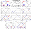 |
Fig. A.1. Radial velocity solutions based on the CRÉME (red and blue points) and literature (grey) measurements. Phase 0 is set to TP – the time of pericentre passage (for e > 0) or quadrature (for e = 0). A141235 and A180413 are SB1 systems with secondary (cooler) components visible. Solution for RZ Eri was re-done using RVs from Popper (1988) and Merle et al. (2024), and TESS photometry. The panel for SZ Cen was created from the original values taken from Andersen (1975). The observations of BQ Aqr are the same as in Ratajczak et al. (2016), but the model has been refined. |
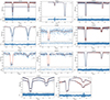 |
Fig. A.2. New and updated light curve solutions, based on TESS or ASAS photometry. Phase 0 is set to T0 – the mid-point of the deeper eclipse. The base level of the SAP flux may change between sectors (e.g. AL Ari, A151848). For SZ Cen, the nonphysically deep eclipses (S11, 1800 s cadence) are caused by overestimated level of third light contamination used in the QLP processing. Please note a different range of phases on the RZ Eri panel. |
A183946 was found to harbour a δ Scuti-type pulsator, whose major pulsation frequency was determined to be fpuls = 9.4255 d−1 (Ppuls = 0.106095 d) with the amplitude of 0.663 mmag (TESS band, not corrected for the companion’s flux). Other frequencies were also noted, but were much weaker, and their analysis is out of the scope of this paper. Another potentially interesting targets are A151848 with a low-mass (0.72 M⊙) secondary, and A084011 residing in the PLATO’s LOPS2 field.
Orbital and physical parameters of the studied systems.
A.1. Notes on individual systems
A.1.1. AL Ari
This is by far the best-studied system in our sample, with very precise physical and stellar parameters available in literature (Graczyk et al. 2021, and references therein). It was therefore a test-bed for our methodology. We used more RV points (Table 2), gathered over a much longer time span (8 years), and photometric time series from TESS observations only. On the other hand, the HARPS RVs used by Graczyk et al. (2021) are the most precise ones that are available, and their ground-based photometry is multi-band and dates back to 1997, also offering a long time base when combined with RVs. With our data we could not, however, confirm their RV acceleration rate of the baricentre (0.056±0.011 ms−1d−1), and found it to be indistinguishable from zero (0.03±0.04 ms−1d−1). We do see hints of the apsidal motion (9.4±7.2 °d−1), and our slightly longer orbital period confirms the Ṗ = 3.8 × 10⁻⁷ d yr−1 value reported in Graczyk et al. (2021).
Both Graczyk et al. (2021) and us reached sub-% precision in stellar masses and radii, together with a very good agreement. Precision in M is about 2 times better in the former work (due to the use of HARPS data only), while we reached lower uncertainties in R (thanks to the TESS photometry). Good agreement is also reached in atmospheric parameters, which is important for understanding potential discrepancies with isochrones. The comparison is shown in Table A.2.
The pair is composed of two Main Sequence (MS) stars. The companion (secondary), which is about 10% smaller and less-massive than the Sun, appears to have its radius overestimated with respect to the models. Such situation is very often observed in active K- and M-type components of DEBs, and is most likely related to rotation and enhanced stellar activity (López-Morales & Ribas 2005; Charbonneau 2014). Problems with age determination in such systems are not uncommon (e.g. Popper 1997). It is also the most likely scenario here, as the TESS light curve of AL Ari shows small-scale, spot-like modulations outside of the eclipses, and the components appear to rotate synchronously. When looking for a common isochrone, we could not find a satisfactory solution, therefore we decided not to include the secondary’s radius as a constraint in the isochrone fitting process (Fig. 3). Despite that the fit led to a satisfactory solution, and good precision in age determination (< 10%).
A.1.2. RZ Eri
This pair is composed of a red giant (RG) spectroscopic component and a companion at the end of its MS evolution or just at the beginning of the sub-giant phase (for simplicity we will call it the MS star). In the RV solution, the latter is formally the more massive star, but, until recently, the large relative errors allowed for solutions where the RG was more massive, as expected in undisturbed evolution scenario. Recent RV data from Merle et al. (2024) showed, however, that the RG truly is the lower-mass star. The RG star is active and spotted, which can be deduced from the out-of-eclipse brightness modulation and asymmetric and variable shape of the secondary eclipse (transit, see Fig. A.2). Such distortions occur when a smaller companion passes in front of cold spots on the surface of the background star (Lurie et al. 2017; Hełminiak et al. 2021). It clearly affected our results, and hampered the precision in radii down to ∼1.6% level. Still, this is a significant improvement with respect to previous studies (Popper 1988; Burki et al. 1992; Vivekananda Rao et al. 1994, Tab A.2).
The leading explanation of the lower mass of the RG component is that it has lost a substantial amount of mass some time in the past. Eggleton & Yakut (2017) estimated that it must have been ∼20 times the amount expected from stellar winds driven by a magnetic dynamo. This would explain the unexpectedly high extinction towards RZ Eri, which was shown to be caused by circumstellar, rather than interstellar material (Burki et al. 1992). Another observational features that favour a disturbed evolution are the rotational velocities: the RG seems to rotate slower than the expected pseudo-synchronisation rotation speed5, while the MS star spins significantly faster. The latter fact could possibly be explained by a Roche lobe overflow (RLOF) from the spectroscopic component, and thus a transfer of mass. Although for such scenario one needs to take into account the size and shape of the relative orbit (a = 72.6 R⊙, e = 0.37).
Comparison of our results with the literature.
The observed properties of RZ Eri, that is the circumstellar material, age inconsistency, and fast rotation of the companion, can also be explained if the companion was a product of a stellar merger. The system would have to have formed as a compact hierarchical triple (CHT), with a short-period inner binary, and a tertiary on a long-period but still relatively tight, significantly eccentric orbit (in line with the currently observed one). Due to dynamical influence of the tertiary (now the RG star), the inner binary’s orbit have been tightened and components have coalesced. Mergers in tertiaries have been proposed to explain the observed properties of the binary HD 148937 (Frost et al. 2024) or blue stragglers with companions (Glebbeek & Pols 2008). Numerous CHTs are now being discovered and characterised (Mitnyan et al. 2024; Moharana et al. 2024), and their dynamical interactions studied (Toonen et al. 2020). Gravitational influence of the outer star can also accelerate the merger (Moharana et al. 2023), especially when it evolves out of the main sequence, and distribution of the angular momenta in the system is changing. Population and statistical studies of mergers in triple systems have been performed (e.g. Kummer et al. 2023; Shariat et al. 2024, and references therein), and the current properties of RZ Eri (e.g. P and e) match some of the outcomes, as well as blue straggler binaries found in clusters (see e.g. Fig. 5 in Shariat et al. 2024). The RG star itself could still be largely intact during the process, or has lost some mass through a tertiary or wind Roche lobe overflow (TRLOF or WRLOF). On a P ∼ 40 d (a ∼ 73 R⊙) orbit it would most likely disturb the material ejected in the collision.
Study of the merger hypothesis is out of the scope of this paper. We find it, however, an interesting alternative to the enhanced mass loss scenario. Confirmation of the merger would require extensive dynamical and evolutionary simulations, as well as dedicated observations to search for the possible remnants. The tracers of the past merger could be identified in spectra of the MS star or the circumstellar medium, after a careful deconvolution of a series of spectra. Unfortunately, this has not been performed so far, and the data describe by Merle et al. (2024) may be insufficient. The merger remnant could also be visible in radio or sub-mm observations.
In case of RZ Eri we were looking for two isochrones independently, assuming that evolution of only one component was undisturbed (which may still not be the case). In the RG mass loss scenario, we found that the age of the MS star is  Gyr, and [Fe/H]init = −0.35 ± 0.15 dex. Additionally, the evolutionary stage of the companion allows to put some constraints in its effective temperature. Under the RG mass loss scenario we found it to be
  K. In the merger scenario, the age of the RG is
  Gyr, and [Fe/H]init = −0.30 ± 0.20 dex. Those two isochrones are presented in Fig. 4.
Even though in this case we could not show the usefulness of totality spectra for determination of the binary’s age, our UVES spectrum and LC+RV solution give important results for this interesting binary. The spectral analysis, which here provided [Fe/H] and Teff of the RG star, has been done for this system for the first time, while the obtained masses and radii are the most precise so far. We plan a further investigation of this object.
A.1.3. A084011
This system is composed of a sub-giant (sG) spectroscopic component with a MS companion. Similarly to RZ Eri, uncertainty in masses is relatively large (5.2 and 3.8%) but for A084011 it is probably because of systematic errors occurring from a low number of observations around the second quadrature (Fig. A.1). With a couple of additional data points between phases 0.65 and 0.95 it should be possible to improve the mass errors down to sub-% level. It may be important in the context of the PLATO mission, as A084011 resides in LOPS2, the first field to be observed.
During the isochrone fitting we encountered a systematic discrepancy between isochrone-predicted values of distance (∼403 pc) and the Gaia DR3 value (454 pc). With the parameter RUWE = 1.055, and no entry in the "Non-Single stars" part of the DR3, the Gaia solution seems to be reliable. But in our fits, no model within the accepted boundaries around the measured stellar parameters, even without spectroscopic ones, has been found to predict distance larger than 445 pc. Therefore, in the final results we decided not to use the distance as a constraint. This discrepancy, although not very strong, remains real and difficult to explain. One possibility is a systematic error in one or two of the observed magnitude values given in SIMBAD, which affected the linear fit to the distance moduli. Another explanation might be an overestimated value of [M/H] obtained in iSpec. Lower metallicity would mean higher effective temperatures and luminosities, thus the stars should be further away from Earth in order to have the same observed brightness.
A.1.4. SZ Cen
This system hosts the hottest spectroscopic component in our sample, and also one of the most massive. SZ Cen is also considered a well-studied system, although the RV and LC solutions were obtained in the 70s (Andersen 1975; Gronbech et al. 1977). The historic RV measurements (Fig. A.1) are all clustered around quadratures, which for a circular orbit is usually sufficient to provide precise and accurate results (here: ∼1.2% for both components). The TESS photometry was available only from the full-frame images (FFIs) from sectors 11 and 38, and was extracted with the TESS Quick Look Pipeline (QLP; Huang et al. 2020). As can be seen in Fig. A.2, this caused some problems during the modelling. SZ Cen lays in a field near the Galactic plane (b ≃ 3.5°), and the QLP severely over-estimated the contamination from background sources (i.e. the third light). One can note that the eclipses from sector 11 are too deep, both reaching 1 mag, which means that much more than 50% of the total flux is being blocked twice. Such situation is physically impossible. During LC modelling a negative value of the l3 parameter had to be used, in order to compensate for the third light over-correction. We found (negative) l3 to be at the level of 42.5 and 9.6% for sectors 11 and 38, respectively. Fortunately, the crucial parameters (r1, r2, i, etc.) were in a good agreement between sectors, and the final values of stellar parameters are also in a good agreement with the literature.
However, one important parameter that was most likely affected was the flux ratio in TESS band. We could not find a satisfactory isochrone fit when lcomp/lspec was included. Similarly to A084011, we could also not reproduce the Gaia distance (diso ≃ 660 pc, vs dGDR3 ≃ 500 pc). The final age and [Fe/H]init estimates were thus found without constraints on flux ratio and d (Fig. 3).
SZ Cen seems to be composed of an sG spectroscopic component with a main sequence companion, which is just at the end of its MS evolution. Some solutions on the earlier stage, for a bit lower EEP mass, are formally acceptable, but they correspond to significantly lower Teff of the companion, and even negative values of E(B − V). Both our temperature estimates are in general agreement with values obtained by Gronbech et al. (1977) from colour indices, which supports our solution. Notably, both Andersen (1975) and Gronbech et al. (1977) reported problems with fitting a single isochrone. Our fit could perhaps been better with more precise masses coming from new RV measurements, and a 120 s cadence TESS photometry from postage stamps (SAP or PDC_SAP), instead of FFIs. Despite the drawbacks, the precision in mass is good, the precision in radii and temperatures is improved with respect to previous studies (Table A.2), and the age determination seems to be secure and reliable. The case of SZ Cen shows that the results from several decades ago may not be enough for the needs of modern stellar astrophysics, and some targets may need to be re-examined.
A.1.5. A141235
This SB1 system has the longest orbital period in our sample, and is possibly the most distant target (dGDR3 = 3374 pc), but the RUWE parameter of its astrometric solutions is quite high (∼2.5). Our accepted models did not reproduce such a large distance (diso = 1530 pc), therefore the distance was not included into the set of constraints in the isochrone fit.
Unfortunately, other parameters, both the spectroscopic and LC-based have relatively large uncertainties, thus they provide rather weak bounds for the models. Still we were able to deduce that the spectroscopic component is an evolved RG, the largest single star in our sample ( R⊙), most likely at the tip of the RG branch (TRGB; Fig. 5). Models with this component being already at the asymptotic giant branch (AGB) are formally not discarded, however less likely, due to the constraint of flux and radii ratios.
A.1.6. A151848
A151848 is a pair of two MS stars, of G and K spectral types. The (spectroscopic) primary is about to turn into a sub-giant. Both components appear to be active, and the (secondary) companion has the lowest stellar mass in our sample. This feature makes the system potentially interesting for further studies on low-mass stars. As in the case of AL Ari, the secondary’s radius seems to be larger than the isochrones predict (∼6σ discrepancy), and thus it was not used as the constraint. Another similarity is the mass of the spectroscopic (more massive) component: 1.175 (A151848) vs 1.164 M⊙ (AL Ari). The latter has significantly smaller radius, which suggests a younger age. Despite the activity, the precision in radii is quite good (∼0.7% for both components), but in masses is significantly lower (2.0+3.3%). This is mainly due to low number of RV points (6 per component) and will surely improve with more data.
Apart from the one radius, the best-fitting model reproduces other parameters quite well. We found a good solution for an age of ∼5 Gyr, which makes A151848 the oldest system in our sample (as suggested by the comparison with AL Ari).
A.1.7. A161710
This is an SB2 with ASAS photometry only. The (spectroscopic) secondary is a RG at the end of the Hertzsprung gap, while (companion) primary is at the MS stage. Large rotational velocity increases the rms of the RVs and, subsequently hampers precision of the RV-based parameters. The quality of ASAS photometry is far from the optimal, thus the LC-based parameters also have large errors. At the end we reach 3.9 and 2.0% fractional error in masses, and 7.1+1.2% in radii, with the lower values for the RG star. Despite the uncertainties, we obtained a good isochrone fit, and secure estimates of age and evolutionary status of both components.
A.1.8. A180413
The TESS photometry available to date for of this binary covered only a single primary eclipse. Therefore, similarly to A141235, for this SB1 system we only used the ASAS photometry, but the RVs were fitted simultaneously with JKTEBOP, because they much better constrain the small but statistically significant eccentricity.
The results of the spectroscopic analysis of the totality spectrum allowed for stronger constraints in the isochrone fit than for A141235. The spectroscopic component is clearly a RG star, while the unseen companion is most likely still a MS object. Both companions of A180413 and A141235 actually show very similar values of stellar parameters. Both systems also seem to be in a similar age. The GDR3 distance of A180413 is well established, and our model reproduces it very well. We must note that the log(g) value of the best-fitting model (2.61 dex) is 3.4σ away from the iSpec value (2.98±0.11 dex). It is possible that the iSpec value is thus over-estimated. For this reason it has not been used in the final isochrone fit.
A.1.9. A183946
This is a pair of two MS stars. The spectroscopic component is almost as hot as the one in SZ Cen. The masses of both stars are well established (0.7+0.5% fractional error), so are the radii (0.6+0.3%). The parameters of the (spectroscopic) primary suggested that it lays in γ Doradus and near δ Scuti instability strips. Indeed the TESS light curve revealed pulsations dominated by a single frequency of 9.4255 d−1 and amplitude of 0.663 mmag, which fits to the latter category of pulsating stars. Other frequencies were also noted, although with a significantly lower amplitude. The best-fitting model reproduces the measurements and observations in a satisfactory way with quite small age uncertainty.
A183946 is therefore a rare case of a DEB with a δ Scuti type pulsator, and very precise and accurate determination of many key parameters, including effective temperature, metallicity, and age.
A.1.10. A191947
Another system with a colder sG or RG spectroscopic component, and an earlier type companion. Large rotational velocities and low number of spectra, especially for the companion, were the most likely causes of relatively large errors in masses (3.1+2.2%). The light curve does not show significant activity-induced variations, so the precision in radii is better (0.9+1.0%). Of all the parameters obtained with iSpec, the ones of A191947 had the largest uncertainties, which later manifested in large uncertainties in age and [Fe/H]init determination. The age-metallicity degeneration is the strongest in our sample, even when the spectroscopic constraints are taken into account (Fig. 6).
The well-established radius of the spectroscopic component is the main constraining factor for its evolutionary phase (it is unlikely that this component is at the horizontal branch) and thus the age of the system. Another strong bound comes from the flux ratio. Its best-fitting model agrees with mass and Teff measurement only at 1.5σ level (Fig. A.3). Despite the aforementioned drawbacks, the isochrone-based distance to A191947 is in a good agreement with the GDR3 result.
A.1.11. BQ Aqr
We initially relied on the solution from Ratajczak et al. (2016), especially for RV-based parameters, but the recent TESS data from Sector 69, when compared with S02, showed that the orbital period value must be shorter. We found new value of P from TESS S02+S69 data, and repeated the V2FIT analysis on the literature RV measurements.
The spectroscopic component of BQ Aqr is an active sG or RG, while the companion is an MS star, right at the end of this evolutionary phase (as the companion in SZ Cen). This system shares some general characteristics with RZ Eri and A084011, but the light curve of BQ Aqr shows the strongest spot-originated modulation in our sample (Fig. A.2). From the shape of the secondary eclipse (i.e. number and location of spot-crossing events) we conclude that there are at least two cold spots, which in their maximum visibility reduce the flux of the active component by ∼23%, and the total flux of the system by ∼16%. With the distorted secondary eclipses and such variation of the flux coming from one of the stars, the LC-based parameters were not found with a good precision. Especially affected were the flux ratio, and the companion’s radius. The final fractional errors in radii were 0.9+4.6% for the spectroscopic and companion components, respectively. Activity, together with high vsin(i), also hampered the RV measurements of Ratajczak et al. (2016), and, subsequently, their and our mass errors (1.8+3.5% here).
Finding the best-fitting model also turned out to be problematic. None of the accepted models could reproduce the GDR3 distance (497±4 pc), thus this parameter was not used as a constraint. The adopted model is in 2-3σ agreement with several measurements (e.g. Mspec, Teff, spec, Rcomp).
We note that our adopted model predicts very high temperature of the companion (7400 K), much higher than the result of SME analysis by Ratajczak et al. (2016) (6390±230 K; Tab A.2). We suspect the reason for this discrepancy is twofold. First, we obtained significantly lower metallicity, which correlates with temperature in spectral analysis. This has been discussed in Sect. 4.2. Second, our determination of the flux ratio may still be inaccurate due to the spots. Without lcomp/lspec in the isochrone fit, we get Teff, comp = 6800(220) K, which is about 1.3σ away from Ratajczak et al. (2016). The best-fitting model in this approach predicts lspec/lcomp = 3.15(63) (≡l2/l1 in Table A.1), [Fe/H]init = −0.15(5) dex,  Gyr, and diso = 618(10) pc. BQ Aqr remains a problematic target, without a satisfactory, self-consistent solution.
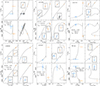 |
Fig. A.3. Same as Fig. 3, but for SZ Cen, A151848, A161710, A183946, A191947, and BQ Aqr. Note that for A161710 the lcomp/lspec is for ASAS V, not the TESS band. |
Appendix B: Test of the light curve fitting approach
Despite JKTEBOP is a widely used light curve fitting code, it is still a simple geometric approach with some limitations, especially when it comes to short-period eclipsing binaries with prominent ellipsoidal variations. The typical “rule of thumb” limit for application of JKTEBOP is that the oblateness of the star should not exceed 4% (Popper & Etzel 1981), and the fractional radius should be smaller than 0.25, above which the resulting radius may be wrong by more than 1% (North & Zahn 2004). This is because the shapes of stars in JKTEBOP are approximated by spheres for calculating eclipse shapes, and as bi-axial ellipsoids for calculating proximity effects, while in more sophisticated codes, like the WD (Wilson & Devinney 1971) or the PHysics Of Eclipsing BinariEs (PHOEBE; Prša & Zwitter 2005; Conroy et al. 2020) it is dictated by the Roche geometry. Since our cases reach and slightly exceed the boundaries cited above, we decided to verify our results, especially how much our radii may be affected by the use of simplified stellar shapes.
We would like to stress that no general conclusions about the use of JKTEBOP should be made on the basis of our tests. These are meant only to verify our most extreme examples.
The approach to model a light curve of a DEB with stronger ellipsoidal variations, by applying JKTEBOP with additional sines and polynomials, has been tested with synthetic data. We used the latest version (v2.4) of PHOEBE to generate light curves of DEBs with substantial ellipsoidal variations. We based our synthetic binaries on three of our systems with TESS photometry available, and largest oblatenesses and fractional radii in the sample (given respectively in parentheses): SZ Cen (2.3%, 0.251), A191947 (4.4%, 0.326), and BQ Aqr (3.4%, 0.290). We added a DEB based on the well-studied AL Ari to ensure the procedure works correctly. We provided the code with input stellar parameters (i.e. M, R, Teff, P, T0) from Tables A.1 and 4, and used exactly the same times of observations as in real TESS curves. Finally, we added white noise corresponding to the rms of the LC fit.
These synthetic curves were analysed with JKTEBOP in the same way as described in Sect. 4.1, including sine functions and polynomials, and errors estimated with a Monte Carlo procedure (Task 8). The MC errors may themselves be lower than the true precision, since they refer to single-sector cases, and do not include scatter between results obtained for different TESS sectors. The resulted values of inclination (i) and fractional radii (r1 and r2) are compared to their input values in Fig. B.1. One can see that JKTEBOP managed to reproduce input values of r1, 2 with accuracy better than 0.7%, exceeding 0.5% in only two cases (secondaries of A191947 and BQ Aqr). Individual discrepancies are better than or comparable to the uncertainties quoted in Table A.1. We thus conclude that JKTEBOP produced reliable results for the studied cases.
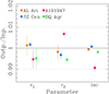 |
Fig. B.1. Comparison of results of the JKTEBOP analysis of synthetic light curves with the input values, for a sample of crucial parameters (fractional radii and inclination). The plot shows ratio of the output to the input value, with scaled uncertainties calculated with Monte-Carlo approach (Task 8). Each colour codes the analysis of a synthetic curve based on one of the selected systems. The dashed vertical lines mark ±1% deviation from the input. In every case, including those with the largest oblateness, JKTEBOP reproduced the input values with accuracy better than 0.7%. |
All Tables
Basic information about targets and log of the UVES observations made during total eclipses.
Atmospheric parameters of ‘spectroscopic’ components of the studied systems, obtained from iSpec analysis of the UVES spectra.
All Figures
|
Fig. 1. Fragments of spectra of studied objects: observed, taken during total eclipses (black), and synthetic (red) created with iSpec from parameters listed in Table 4. All spectra are corrected for the barycentric and radial velocities and normalised to the continuum. They are plotted in the same scale to emphasise differences between them. |
| In the text | |
|
Fig. 2. Graphical explanation of distance and reddening determination method. The distance moduli (m − M)λ, calculated from observed magnitudes and synthetic photometry in different bands, are plotted (black dots) as a function of their corresponding law coefficient, by which we define the applied extinction law. The slope and the intercept of the fitted line (solid black) are the values of E(B − V) and reddening-free distance modulus (m − M)0, respectively. The (m − M)0 level is shown in blue. Differences between (m − M)0 and each (m − M)λ represent extinction values Aλ in each band (in mag), and they are also labelled. |
| In the text | |
|
Fig. 3. Comparison of parameters of SB2 systems with isochrone (black line) containing best-fitting model (open square symbols for two components). Age and initial metallicity for the isochrone are given, together with the predicted distance. Measurements and indirect determinations of stellar parameters are marked with filled dots with error bars, and their associated models are marked with open squares. Components labelled ‘spectroscopic’ are represented with orange symbols, while the ‘companions’ are shown with light blue ones. For each object, we show M − R, lcomp/lspec − R, M − Teff, and lcomp/lspec − Teff panels. On the lcomp/lspec panels, the isochrones were scaled with respect to the absolute magnitude of the model that matches the ‘spectroscopic’ component; thus, it is by definition located on the grey dashed line that marks the unity. In cases where a certain parameter was not used as a constraint in the fitting process (e.g. Rcomp for AL Ari or lcomp/lspec for SZ Cen), its model values from all the accepted isochrones are shown with grey dots. Zoomed-in images of the vicinity of the determined parameters were drawn for clarity in the insets. Here, we show results for AL Ari and A084011, while other systems are presented in Fig. A.3. |
| In the text | |
|
Fig. 4. Isochrones fitted to the components of RZ Eri separately, shown only on the M − R (left) and M − Teff (right) planes. The isochrones are labelled with their age (in gigayears) and initial metallicity. Colour-coding for the components is the same as in Figs. 3 and A.3. |
| In the text | |
|
Fig. 5. Same as Figs. 3 and A.3, but for SB1 systems (top: A141235; bottom: A180413) and on different planes. We only show Teff − log(g) (left) and lcomp/lspec − Rcomp/Rspec (right). On the latter, the spectroscopic component is shown without errors, and set by definition to (1.0;1.0). Flux ratios refer to the ASAS V band. |
| In the text | |
|
Fig. 6. Graphical presentation of age-metallicity degeneration in isochrone fitting of the studied systems on the [Fe/H]init vs. log(τ) planes. Orange symbols represent the accepted isochrones in fits constrained only by the RV+LC (for SB2s) or LC-based (for SB1s) parameters. Blue points are accepted isochrones after including spectroscopy in the set of constraints. The white stars mark the isochrones that contain the best-fitting models. Significant reduction in allowed ages and initial metallicities is clearly seen in almost all cases, even when spectroscopic parameters were not well constrained. The SB2 systems are shown on the top three rows (without RZ Eri), while the two SB1 systems are shown in the lowest one. |
| In the text | |
|
Fig. 7. Determination of stellar age through isochrone fitting for cases with and without spectroscopic constraints. The grey dotted line on each panel shows the equality relation (y = x). Left: Logarithm of age (log(τ)). Uncertainties from each approach are shown with different colours for easier comparison. Centre: Uncertainties in age Δlog(τ) defined as 16th-to-84th percentile or ±1σ ranges. Right: Comparison of best-fitting initial metallicities [Fe/H]init. |
| In the text | |
|
Fig. A.1. Radial velocity solutions based on the CRÉME (red and blue points) and literature (grey) measurements. Phase 0 is set to TP – the time of pericentre passage (for e > 0) or quadrature (for e = 0). A141235 and A180413 are SB1 systems with secondary (cooler) components visible. Solution for RZ Eri was re-done using RVs from Popper (1988) and Merle et al. (2024), and TESS photometry. The panel for SZ Cen was created from the original values taken from Andersen (1975). The observations of BQ Aqr are the same as in Ratajczak et al. (2016), but the model has been refined. |
| In the text | |
|
Fig. A.2. New and updated light curve solutions, based on TESS or ASAS photometry. Phase 0 is set to T0 – the mid-point of the deeper eclipse. The base level of the SAP flux may change between sectors (e.g. AL Ari, A151848). For SZ Cen, the nonphysically deep eclipses (S11, 1800 s cadence) are caused by overestimated level of third light contamination used in the QLP processing. Please note a different range of phases on the RZ Eri panel. |
| In the text | |
|
Fig. A.3. Same as Fig. 3, but for SZ Cen, A151848, A161710, A183946, A191947, and BQ Aqr. Note that for A161710 the lcomp/lspec is for ASAS V, not the TESS band. |
| In the text | |
|
Fig. B.1. Comparison of results of the JKTEBOP analysis of synthetic light curves with the input values, for a sample of crucial parameters (fractional radii and inclination). The plot shows ratio of the output to the input value, with scaled uncertainties calculated with Monte-Carlo approach (Task 8). Each colour codes the analysis of a synthetic curve based on one of the selected systems. The dashed vertical lines mark ±1% deviation from the input. In every case, including those with the largest oblateness, JKTEBOP reproduced the input values with accuracy better than 0.7%. |
| In the text | |
Current usage metrics show cumulative count of Article Views (full-text article views including HTML views, PDF and ePub downloads, according to the available data) and Abstracts Views on Vision4Press platform.
Data correspond to usage on the plateform after 2015. The current usage metrics is available 48-96 hours after online publication and is updated daily on week days.
Initial download of the metrics may take a while.