| Issue |
A&A
Volume 692, December 2024
|
|
|---|---|---|
| Article Number | A110 | |
| Number of page(s) | 15 | |
| Section | Stellar structure and evolution | |
| DOI | https://doi.org/10.1051/0004-6361/202451720 | |
| Published online | 03 December 2024 | |
Precise physical parameters of three late-type eclipsing binary giant stars in the Large Magellanic Cloud
1
Nicolaus Copernicus Astronomical Centre, Bartycka 18, 00-716
Warsaw, Poland
2
Nicolaus Copernicus Astronomical Centre, Rabiańska 8, 87-100
Toruń, Poland
3
Departamento de Astronomía, Universidad de Concepción, Casilla 160-C, Concepción, Chile
4
Carnegie Observatories, 813 Santa Barbara Street, Pasadena, CA 91101-1292, USA
5
Astronomical Observatory, University of Warsaw, Al. Ujazdowskie 4, 00-478
Warsaw, Poland
6
Department of Physics and Astronomy, Uppsala University, Box 516
SE-751 20
Uppsala, Sweden
7
Leiden Observatory, Leiden University, P.O. Box 9513
2300 RA
Leiden, The Netherlands
⋆ Corresponding author; This email address is being protected from spambots. You need JavaScript enabled to view it.
Received:
30
July
2024
Accepted:
21
October
2024
Abstract
Context. Detached eclipsing binaries (DEBs) allow for the possibility of a precise characterization of their stellar components. They offer a unique opportunity for deriving their physical parameters nearly independent of a model for a number of systems consisting of late-type giant stars. We aim to expand the sample of low-metallicity late-type giant stars with precisely determined parameters.
Aims. We determine the fundamental parameters, such as the mass and radius, or the effective temperature for three long-period late-type eclipsing binaries from the Large Magellanic Cloud: OGLE-LMC-ECL-25304, OGLE-LMC-ECL-28283, and OGLE-IV LMC554.19.81. Subsequently, we determine the evolutionary stages of the systems.
Methods. We fit the light curves from the OGLE project and radial velocity curves from high-resolution spectrographs using the Wilson-Devinney code. The spectral analysis was performed with the GSSP code and resulted in the determination of atmospheric parameters such as effective temperatures and metallicities. We used the isochrones provided by the MIST models based on the MESA code to derive the evolutionary status of the stars.
Results. We present the first analysis of three DEBs composed of similar helium-burning late-type stars that pass through the blue loop. The estimated masses for OGLE-LMC-ECL-29293 (G4III + G4III) are M1 = 2.898 ± 0.031 and M2 = 3.153 ± 0.038 M⊙, and the stellar radii are R1 = 19.43 ± 0.31 and R2 = 19.30 ± 0.31 R⊙. OGLE-LMC-ECL-25304 (G4III + G5III) has stellar masses of M1 = 3.267 ± 0.028 and M2 = 3.229 ± 0.029 M⊙ and radii of R1 = 23.62 ± 0.42 and R2 = 25.10 ± 0.43 R⊙. OGLE-IV LMC554.19.81 (G2III + G2III) has masses of M1 = 3.165 ± 0.020 and M2 = 3.184 ± 0.020 M⊙ and radii of R1 = 18.86 ± 0.26 and R2 = 19.64 ± 0.26 R⊙. All masses were determined with a precision better than 2% and the precision for the radii is better than 1.5%. The ages of the stars are in the range of 270–341 Myr.
Key words: binaries: eclipsing / binaries: spectroscopic / stars: evolution / stars: fundamental parameters / stars: late-type
© The Authors 2024
 Open Access article, published by EDP Sciences, under the terms of the Creative Commons Attribution License (https://creativecommons.org/licenses/by/4.0), which permits unrestricted use, distribution, and reproduction in any medium, provided the original work is properly cited.
This article is published in open access under the Subscribe to Open model. This email address is being protected from spambots. You need JavaScript enabled to view it. to support open access publication.
1. Introduction
A most remarkable feature of double-lined detached eclipsing binaries (DEB) is that their stellar and orbital parameters can be determined with high precision from observations and empirical calibrations alone, without many model assumptions. For this reason, DEBs serve as an important tool in a wide range of topics in stellar astrophysics, especially as a fundamental source of measurements of the stellar radii and masses (e.g. Torres et al. 2010; Southworth 2015; Eker et al. 2018). They are very useful for testing stellar evolution codes (e.g. Higl & Weiss 2017; del Burgo & Allende Prieto 2018) and also for calibrating relations in asteroseismology (Gaulme et al. 2016) as well as surface-brightness relations (Graczyk et al. 2021), among others. During the past two decades, DEBs continued to rise in prominence when it was shown that they allowed for near-geometrical, one-step distance measurements to the Milky Way globular clusters (e.g. Thompson et al. 2001; Rozyczka et al. 2022) and the Local Group galaxies (e.g. Bonanos et al. 2006; Vilardell et al. 2010; Pietrzyński et al. 2013; Graczyk et al. 2014). This use of DEBs was already envisioned by Paczynski (1997) who proposed that DEBs might be well-suited for measuring model-independent extragalactic distances with a precision to within 1%. This ambitious goal was achieved for the Large Magellanic Cloud (LMC; Pietrzyński et al. 2019) with a sample of unique DEBs that consisted of two late-type giant stars.
In total 20 late-type giant DEBs were analyzed and characterized in the LMC (Graczyk et al. 2018) and 15 such systems in the Small Magellanic Cloud (SMC, Graczyk et al. 2020). The components of these DEBs are a mixture of red giant branch stars, horizontal branch stars, and hot asymptotic branch stars. These binary systems are rare because 1) their initial separation must be large enough to accommodate components within their Roche lobes because they swell on the red giant branch, and 2) the mass ratio of components must be close to unity so that two giant stars can be observed at the same time. The systems from the LMC were used not only for a distance determination, but also to determine the geometry of the LMC disk (Pietrzyński et al. 2019) and the age-metallicity relation in the LMC (Graczyk et al. 2018), and to constrain the convective core-overshooting in intermediate-mass stars (Claret & Torres 2019). Using published OGLE catalogs of eclipsing binary stars in the LMC (Graczyk et al. 2011; Pawlak et al. 2016), we commence a search for additional late-type giant DEBs in the LMC. The main aim is to expand the sample of DEBs that are suitable to constrain the disk geometry better and to eventually improve the precision of the distance determination to the LMC. The importance of this galaxy is that it is one of only three geometric anchors of the extragalactic distance scale (e.g. Riess et al. 2022).
We determine the fundamental physical parameters for three new DEBs consisting of late-type giant stars. All are members of the LMC: OGLE-LMC-ECL-29293, OGLE-LMC-ECL-25304, and OGLE-IV LMC554.19.81 (hereafter LMC29293, LMC25304 and LMC554, respectively). All three eclipsing binaries are well detached and show deep partial eclipses. Their orbits are circular or only slightly eccentric.
The structure of this work is the following: in Sect. 2 we present the observational data source we used to model our systems. Section 3 contains information about the radial velocity determination from the spectroscopic data. In Sect. 4 we describe our handling of the reddening to the sources and estimate their preliminary temperatures. Section 5 describes our strategy for a solution to the radial velocity and light curves of the systems. We determine the atmospheric parameters from the disentangled stellar spectra in Sect. 6. The adopted solutions for each DEB are described in Sect. 7. In Sect. 8 we determine the evolutionary stage and age of the systems. Section 9 contains our conclusions.
2. Observations and data
The basic information about the targets is summarized in Table 1, and their location on the sky is shown in Fig. 1. The three systems (red circles) were selected because of their long orbital periods and late spectral types. They are located at a relatively large projected distance from the LMC center. The systems were identified through the third and fourth phase of the Optical Gravitational Lensing Experiment (OGLE) (Udalski et al. 1997, 2015; Udalski 2003). The OGLE project has been conducted for more than two decades with the 1.3 m Warsaw Telescope, located at Las Campanas Observatory, Chile. For the analysis performed in this article, we used the published I-band light curves. For one of the objects, LMC554, we present an unpublished I-band light curve from the OGLE-IV phase (Soszyński, private communication). The typical cadence of the I-band light curves is between 1 and 3 days. The V-band light curves are much more sparse, and the light curves in this band are poorly populated. We therefore decided to exclude the V-band light curve from the analysis.
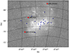 |
Fig. 1. Location of our targets (red dots) in the projection of the Large Magellanic Cloud. The blue dots correspond to the systems studied by Graczyk et al. (2018). The underlying image was obtained by The All Sky Automated Survey and originates from Udalski et al. (2008). |
Preliminary information on the targets.
High-resolution spectroscopic observations of the targets were obtained using three different spectrographs: The Magellan Inamori Kyocera Echelle (MIKE), the Ultraviolet and Visual Echelle Spectrograph (UVES), and the High Accuracy Radial velocity Planet Searcher (HARPS). MIKE is a high-resolution double echelle spectrograph implemented at the Magellan Clay 6.5 m Telescope at Las Campanas Observatory in Chile; a description of this instrument can be found in Bernstein et al. (2003). With this instrument, it is possible to reach a resolution of around R ∼ 40 000. HARPS (Mayor et al. 2003) is another high-resolution spectrograph that is mounted on the 3.6 m telescope at La Silla Observatory in Chile. The observations were performed in the EGGS mode, reaching a resolution about 80 000. The UVES spectrograph is one of the instruments hosted at the 8.4 m UT2 Kueyen telescope, which is a part of the Very Large Telescope (VLT), at Cerro Paranal Observatory, Chile. This instrument can also reach a resolution of about 80 000 in its high-resolution mode. Information on this specific instrument can be found in Dekker et al. (2000).
3. Radial velocity determination
The spectra collected with these instruments were used to determine radial velocity (RV) changes for each source. To achieve this goal, we used the broadening function technique (BF), a formalism introduced by Rucinski (1999). This technique is implemented in the RaveSpan software developed by Pilecki et al. (2013). The determination of the RVs using this approach requires templates from the synthetic stellar spectral library of Coelho et al. (2005). The selection of the templates needs to resemble the atmospheric characteristic of the observed sources in terms of metallicity, logg, and the effective temperature. As a value for the metallicity, we used an average metallicity of the LMC of [Fe/H] = −0.42 dex, as reported by Choudhury et al. (2021). The temperatures were set according to the method described in Sect. 4.
The radial velocities were corrected by an instrumental shift term to account for the use of the three different instruments. This is crucial to ensure consistency by addressing calibration differences, such as those in optical or instrumental setups, and it allows an accurate comparison of the radial velocities. We established the systemic velocity as the one determined from the HARPS spectra, and we then applied shifts to the RV determined from UVES and MIKE spectra. For LMC29293, we shifted the RV determined with MIKE by 2.122 km/s, and to the UVES RV, we shifted it by −2.261 km/s. In the case of LMC25304, we applied a shift of 1.187 km/s to the RV determined with MIKE and 0.299 km/s to those we obtained from the UVES spectra. Finally, in the case of LMC554.19.81, the shift applied to the MIKE radial velocities was 0.5 km/s, and for the UVES spectra, it was 1.140 km/s. The radial velocities corrected for the instrumental shifts are shown in Tables 2, 3, and 4. In the case of MIKE spectra, we only used spectra that were collected with the red arm of the spectrograph (MIKE-Red). We decided to use this region because the S/N is significantly better than for the blue part of spectra.
Radial velocity measurements for the object LMC29293.
Radial velocity measurements for the object LMC25304.
Radial velocity measurements for the object LMC554.
With RaveSpan, we also solved the radial velocity curves to produce estimates of the eccentricity, radial velocity semiamplitudes, arguments of periastron, and systemic velocities. These estimates were used as input parameters for the later analysis.
We determined spectroscopic light ratios in the V band for all systems using the strength of the broadening function peaks. The resulting light ratios were subsequently corrected for the small surface temperature differences of the components. The resulting spectroscopic light ratios are 1.04 ± 0.05, 0.99 ± 0.05, and 1.05 ± 0.04 for LMC29293, LMC25304, and LMC554, respectively. This information subsequently turned out to be useful to better constrain light-curve solutions because photometric light ratios and radii ratios are correlated (see the corner plots in Appendix A).
4. Estimating the reddening and initial temperature
To estimate the initial system temperature, we used the infrared color (V − K) corrected for the interstellar extinction. To obtain the intrinsic colors of the systems, we estimated the interstellar extinction from the LMC reddening maps of Skowron et al. (2021) and Chen et al. (2022). Independently, we derived reddenings from the sodium doublet NaI (5889.951, 5895.924 Å) using the calibrations provided by Munari & Zwitter (1997) and Poznanski et al. (2012). We could only detect multicomponent absorption due to the Milky Way interstellar material (ISM), while any absorption caused by the LMC ISM was below the detection limit. Table 5 summarizes the reddening determination for our three systems, where the mean values are adopted as the final interstellar extinction estimates.
Reddening estimates, E(B − V).
In order to convert the reddening E(B − V) into E(V − K), we used the following relation from (Savage & Mathis 1979):
 (1)
(1)
We used several (V − K) color–effective temperature calibrations to estimate the main effective temperature of our targets, such as di Benedetto (1998), Tokunaga (2000), Houdashelt et al. (2000), Ramírez & Meléndez (2005), González Hernández & Bonifacio (2009), Casagrande et al. (2010) and Worthey & Lee (2011) . We averaged the estimates to obtain the initial mean effective temperature for each system. In the case of LMC29293, we obtained T = 5266 K, for system LMC25304, we obtained T = 4858 K, and for system LMC554, we obtained T = 5325 K.
5. Modeling approach and preliminary solution
In order to determine the physical characteristics of the systems, we used the fitting routine implemented in the Wilson-Devinney (hereafter WD) program (Wilson & Devinney 1971; Wilson 1979, 1990; Van Hamme & Wilson 2007), version 2007. This routine allows us to simultaneously fit light and radial velocity curves. The WD program uses a differential correction algorithm to determine a set of parameters that describe observables. We simultaneously adjusted the I band and the RV curves for each system. Mode 2 of the program was used as it was designed specifically for DEBs, and we set "IPB=0", which coupled the luminosity and temperature for the analysis. The albedo for both components was set to 0.5 and the gravity brightening β to 0.32, which are the standard values for stars with convective envelopes (Lucy 1967). In all of our modeling, the logarithmic limb-darkening law (Klinglesmith & Sobieski 1970) was used with automatically updated coefficients, "LD1=LD2=-2", as well as the stellar atmosphere formulation "IFAT1=IFAT2"=1. We apply proximity and eclipse effects to the radial velocity curves by setting "ICOR1=ICOR2=1". We set the grid integer size as "N1=N2=60" to describe the size of the grid at the surface of the stars, and the noise parameter to "NOISE=1" for observational scatter to scale with the square root of the light level. These settings were intended to optimize the interpretation of the DEB data.
5.1. Initial parameters
The orbital periods and times of primary eclipse minimum were adopted from Pawlak et al. (2016) in the case of LMC29293 and LMC25304. We verified these values using the phase dispersion minimization (PDM) in IRAF1 (Stellingwerf 1978). For system LMC554, the ephemeris was calculated using PDM. The parameters from the RaveSpan RV fit (Sect. 3) were set as the initial orbital parameters for the fitting. The temperature of the primary star was set as the value from the color-effective temperature relations as described in Sect. 4. The metallicity was assumed to be the average metallicity for the LMC (Sect. 3).
5.2. Modeling strategy
The following parameters were adjusted simultaneously: the eccentricity e, the semimajor axis a, the orbital inclination i, the argument of periapsis ω, the surface potentials Ω1 and Ω2, the systemic velocity γ separately for each component, the mass ratio q = M2/M1, the effective temperature of the secondary component T2, the orbital period P, the phase shift ϕ, the light of the primary component in a given filter L1 and also the third light l3. The best solution was identified by a comparison of the resulting χ-squared value calculated by comparing the model to the observed light curves.
During the light-curve modeling, we found that the radii of components r1 and r1 are quite strongly correlated for all three systems. We employed the spectroscopic light ratio in the V band to break the degeneracy between the parameters. The model V band ratios were extrapolated using the LC module of the WD code. After several unconstrained iterations, a solution was found only for LMC25304, in which the model and observed spectroscopic light ratios agree within the uncertainties. However, for LMC29293 and LMC554, we had to fix the potential of the secondary component in order to obtain agreement with the spectroscopic light ratio.
After a satisfactory solution was reached, new light ratios were used to recalculate the effective temperature of the components from the color-effective temperature relations listed in Sect. 4. After this, the WD models were recalculated once again with the new temperatures.
We searched for a third light l3, which might suggest the existence of an additional body that contributes to the total luminosity of the systems, for all systems. We derived very low or negative values of l3. Subsequently, we set l3 = 0 in the case of LMC25304 and LMC554. In the case of LMC29293, we estimated a very weak contribution of third light.
6. Atmospheric parameters
6.1. Spectral decomposition
To identify atmospheric features of our stars from their spectra, such as metallicity, projected rotational velocities, microturbulence, and effective temperatures, the composed spectra, with contributions from both stars, must be disentangled. To this end, we used the González & Levato (2006) prescription implemented in RaveSpan. Only spectra listed as MIKE-Red in Tables 2, 3 and 4 were used, because their S/N is higher. The disentangled spectra are the result of an iterative process consisting of using the computed spectra of one of the stars to calculate the other, and vice versa, subtracting the lines of one of the components with respect to its Doppler shift from the composed spectra at different phases.
6.2. Determining the macroturbulence velocity
In order to derive the atmospheric parameters from the decomposed spectra of our systems, we made some assumptions. The spectral S/N is ∼10 for our systems because the sources are faint. This level of noise might therefore induce a doubtful determination of some parameters. To mitigate this effect, we fixed the surface gravity logg to a dynamical value derived from initial solutions found with the WD code. It is difficult or even impossible to infer the macroturbulence velocity ζ from low S/N spectra because it is strongly correlated with the projected rotation velocity vsini. Thus, we estimated the ζ from the following set of equations given by (Hekker & Meléndez 2007; Massarotti et al. 2008 and Takeda et al. 2008):
 (2)
(2)
 (3)
(3)
 (4)
(4)
We took the average of the three above estimates as the value of ζ. These values were fixed during the subsequent analysis of the decomposed spectra. The calculated values for macroturbulence of each star are listed in Table 6.
Results of the GSSP atmospheric analysis.
6.3. Analysis with the GSSP code
A set of the atmospheric parameters such as the microturbulence velocity ξ in the chromosphere of the stars, the effective temperature Teff, the projected rotational velocity vsini, and the metallicity [M/H] was determined using the software called grid search in stellar parameters (GSSP) published by Tkachenko (2015). This software uses a grid of these parameters and fits the best synthetic spectra to the observed data. The advantage of GSSP is that it is possible to simultaneously fit all aforementioned parameters for both stellar components in a binary configuration. The software computes synthetic spectra using the SynthV LTE-based radiative transfer code (Tsymbal 1996). It also uses a grid of atmosphere models that is precomputed with the LLmodels code (Shulyak et al. 2004), and also with the model atmospheres in a radiative and convective scheme (MARCS), which is a grid of models for late-type stars (Gustafsson et al. 2008).
The general idea is to search for a better fit to the data around the selected input parameter values and to adopt the best set of parameters by calculating the Chi-square of the residuals between the synthetic and the observed spectrum. The spectral region we analyzed was in the range of 5985–6787 Å, because in this spectral region the level of noise is lower than in the bluer spectral regions. We also avoided regions with telluric lines listed by Kurucz (2005), such as O2 around 6300 Å and the H2O lines around 6500 Å. The result of our analysis is presented in Table 6.
7. Adopted solution and calculation of uncertainties
The adopted solution is the combination of the results obtained with the WD code and the spectral analysis performed with GSSP. The final effective temperatures were estimated using the previously mentioned color-effective temperature relations in Sect. 4, applying the light ratios obtained from our WD models to disentangle the individual contribution of each star to the total observed magnitude in a given band. We calculated the arithmetic mean temperature with the GSSP temperature and those from the method mentioned above.
The statistical errors of the parameters were calculated using the JKTEBOP code (e.g. Southworth et al. 2005, 2004). JKTEBOP models and analyzes detached binary systems based on their light and radial velocity curves. The code is based on the EBOP code written by Popper & Etzel (1981) (see also Etzel 1981). JKTEBOP is implemented with a Monte Carlo (MC) algorithm to estimate the uncertainty.
As an input for the JKTEBOP MC analysis, we used the WD model parameters derived in Sect. 5. We assumed that the parameters given by the WD model are a proper representation for the JKTEBOP code, which follows from the fact that all systems are well detached. The MC analysis performed with JKTEBOP works as follows: The adjusted parameters are independently perturbed by low values and compared with the phased observed light curve. The resulting corner plots of the analysis are shown in Appendix A. The outcomes of WD and JKTEBOP were compared in order to verify whether the parameters agreed with each other. The solution we adopted is a combination of the parameters from WD and uncertainties derived with JKTEBOP presented in Table 7.
Orbital and photometric parameters from the adopted solution using the codes WD and JKTEBOP.
The physical parameters were derived using a set of astrophysical constants advocated by Prša et al. (2016), and they are summarized in Table 8. The spectral types were estimated based on the surface temperatures and gravities according to Table 1 from Alonso et al. (1999). Below, we describe individual systems in more detail.
Fundamental and physical properties derived from the adopted solution.
7.1. OGLE-LMC-ECL-29293
LMC29293 is a detached binary composed of two late-type giant stars that are very similar in terms of temperature, radii, luminosity, and masses. Both stars were classified as G4III, and the system is the most metal-rich in our sample ([M/H] = −0.37 ± 0.15 dex). The secondary is the slightly hotter star of the system and is also the more massive component. This description is slightly different from the GSSP results, which prefer the primary star to be slightly hotter, but this might be explained by the relatively low S/N of the analyzed spectra.
The eccentricity of the system is very low (see Fig. 3). We obtained e = 0.002 ± 0.003, and we fixed e = 0 during subsequent analysis. A small amount of third light was detected, but its influence on our solution is insignificant, and we also fixed ℓ3 = 0. The light-curve analysis showed that in an unconstrained WD solution, the radii of the components are strongly correlated, and it was practically impossible to make the parameters converge. We used the spectroscopic light ratio to restrict the light ratio of the components by fixing the secondary surface potential. In this way, we were able to break the degeneracy of the photometric parameters.
This system shows the components with the most unequal masses in our sample; the mass ratio of the remaining two systems is very close to unity, which agrees with the physical similarity of their components. LMC29293 consists of two stars with notably similar external characteristics, but they differ significantly in their masses. We address this problem in Sect. 8.1.
 |
Fig. 2. 6080–6200 Å spectral region of the object LMC25304. The red lines are the disentangled spectra from MIKE-red observations. The black lines are the synthetic spectra generated using the GSSP binary mode. |
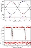 |
Fig. 3. Radial velocity data and their binary solution (upper panel), and the photometric light curve with its solution (lower panel) obtained with the WD code for system LMC29293. The smaller lower panel shows the residuals of our adopted solutions. |
7.2. OGLE-LMC-ECL-25304
The object LMC25304 is an eclipsing binary composed of two similar late-type giant stars. We estimated their spectral types as G4III+G5III. The eclipses are deep and almost central, but no totality phase can be seen (see Fig. 4). The components have the highest masses and largest radii in our sample, alongside the widest separation and significant eccentricity. Additionally, the mass ratio of this system is below 1, meaning that the hotter primary component is slightly more massive than its companion.
During the light-curve analysis, we found a low negative value of the third light in the I band (ℓ3 = −0.0016(89)), and therefore, we set ℓ3 = 0 in our adopted solution. The orbital inclination i of the orbit is so close to 90 degrees that it causes a numerical instability when we solved for it with the WD code. Using Monte Carlo simulations with the JKTEBOP code, we restricted a range of possible inclinations (see Appendix A), and during the subsequent analysis, we fixed the orbital inclination at i = 89.775 deg.
For this system in our sample alone, an unconstrained light curve solution leads to a light ratio that is fully consistent with the spectroscopic light ratio. Subsequently, we did not fix any other parameter during the analysis. The adopted solution does not show any significant systematic residuals. Interestingly, although the system is the brightest in our sample, its I band light curve solution shows the largest rms. We searched for periodicity in the residuals using the phase-dispersion minimization (PMD) method (Stellingwerf 1978) and the Lomb-Scarle periodogram (Lomb 1976; Scargle 1982). Both methods returned the strongest power peaks at frequencies corresponding to one year and one day and their harmonics (Fig. 5). The former is caused by systematic seasonal brightness trends due to airmass changes, while the latter arises from the basic one-day OGLE cadence. However, both effects combined do not explain the residual spread. No other significant frequency peaks were detected; thus, probably one or both components of LMC25304 exhibit some short-term erratic variability that increases residuals.
 |
Fig. 5. Results of the periodicity search in the light residuals of LMC25304. The upper panel shows the PDM diagram, and the lower panel shows the Lomb-Scargle periodogram. |
7.3. LMC554.19.81
This system is composed of the hottest stars in the sample. We estimated their spectral types as G2III+G2III. As in the two previous systems, the eclipses are partial, deep, and well separated. The OGLE I band light curve is of good quality and has the smallest rms in the sample (see Fig. 6). No significant out-of-eclipse variability was observed. No third light was detected, but we found a low but significant eccentricity that reduced the residuals of the WD solution to the light and radial velocity curves.
As in the case of LMC29293, we found a strong correlation between the component radii during the analysis with the WD code. The correlation was not as strong as in LMC29293, but we had to constrain the model light ratio by using the spectroscopic value and fixing the secondary surface potential. In general, the errors on the parameters we obtained for this system were the smallest in the sample.
8. Evolutionary stage
From our solutions, we obtained very well determined masses, radii, luminosities, and effective temperatures for each analyzed star. We also obtained an estimate of the individual abundances of the stars from our spectroscopic analysis. By implementing these values, we were able to construct isochrones for our sources with the aim of determining their ages. We used the MESA Isochrones and Stellar Tracks (MIST) library (see Choi et al. 2016 and Dotter 2016 for details) computed using the code called modules for experiments in stellar astrophysics (MESA) code (Paxton et al. 2011). The MIST models are scaled to the abundance of the Sun and evolve the stars from the ZAMS to later stages of stellar evolution.
For the analysis, we selected a grid of isochrones that covered the range of log(Age) from 8 to 9 in steps of 0.005 dex and corresponded to the spectroscopic metallicities derived with GSSP. We compared the position of our targets in the log(Teff) versus logL/L⊙ plane with the isochrones and checked for consistency with the masses and radii of each component. Since our stars seem to be passing through the same evolutionary stage, it is expected that the formation of the two components occurred at a similar time with an identical initial composition.
For a given age, we selected three isochrones that differed in abundance corresponding to the mean, lower, and upper values for the metallicity of a system given in Table 8. By varying the isochrone age, we searched for the age that minimized the distance between the theoretically predicted and the observed mass, while simultaneously satisfying the position of our stars in the mass versus radius, mass versus luminosity, and mass versus Teff planes. The consistency of our parameters with the theoretical predictions for a certain age is shown in the figures in Appendix B.
For all three cases, we note that our systems must be placed at the so-called blue loop, when stars begin to ignite helium in their helium-rich cores through the triple α process. This causes a star move to a bluer region in the HRD, where it becomes hotter for a period, and it then cools again before it enters the asymptotic giant branch (AGB). Our estimated ages are presented in Table 8.
8.1. OGLE-LMC-ECL-29293
System LMC29293 presents the most complex scenario for an evolutionary analysis in our sample. As previously mentioned, the masses of these stars are the most different from each other of the three systems. On the other hand, both stars are expected to be at the same evolutionary stage since they are very close to each other in the HR diagram (see Fig. 7).
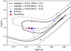 |
Fig. 7. Determination of the age for system LMC29293 with theoretical isochrones (black lines). The dashed gray lines correspond to ±1σ uncertainty limits for the metallicity from Table 8. The blue and red crosses mark the masses and luminosities of the primary and secondary components, respectively. |
The difference in masses indicates that the secondary component, that is, the more massive component, is probably slightly more evolved and already approaches the AGB, while the primary is probably still becoming hotter and just enters its blue loop after passing through the helium flash. According to the proposed evolutionary stage, our system is composed of stars with ages in the range of 8.502 < log(Age) < 8.558, giving a mean age of around 337 Myr. When evolutionary tracks were fit separately for each component, the best-fit ages were different by 62 ± 12 Myr for the same chemical composition.
Several reasons can be invoked to explain why it is not possible to simultaneously fit an isochrone for both stars. The system may be the result of a stellar capture, maybe a former hierarchical triple system in which one of the components is the result of a stellar merger. However, the observed similarity of the components is difficult to explain in both scenarios without assuming some very intricate fine-tuning of the stellar parameters.
Another possible explanation might be differences in the initial rotation rates of the stars, discrepant initial compositions, or an interaction with another star that changed the context of the binary. The system components show the most discrepant surface metallicities in the sample, however, uncertainties are also large and the difference is only slightly larger than 1σ.
8.2. OGLE-LMC-ECL-25304
The comparison with evolutionary models suggests that both stars are at the same evolutionary stage (see Fig. 8). They have just entered their blue loops and become slightly hotter as helium burning occurs at their center. The isochrone that is most consistent with the observed values corresponds to the adopted mean metallicity, [M/H] = −0.6 dex, and the age is  , that is, 260 Myr. Both stars are about 2σ off their predicted position: The difference in their masses suggests a larger difference in the surface temperatures than is actually observed.
8.3. LMC554.19.81
The best solution places the components of the system at the blue edge of the loop on the HR diagram (see Fig. 9). For metallicities close to the system’s mean, that is, [M/H] = −0.45 dex, we obtained fully satisfactory fits and the stars nearly reached their maximum temperature. Both 1σ higher and lower metallicities (i.e., [M/H] = −0.6 and −0.3 dex) give significantly worse fits to the observed position of the components. We estimate the age of the system to be between 8.46 < log(Age)< 8.56, or approximately 280 Myr.
9. Photometric distances
Using the parameters established throughout this work along with individual bolometric corrections from Alonso et al. (1999), we determined the photometric distances by applying the following equation from (Graczyk et al. 2017):
 (5)
(5)
where i = 1, 2 corresponds to the primary and secondary stars, respectively. T is the effective temperature of each star in K, R is their stellar radius in units of solar radii, and V is the intrinsic magnitude of the star corrected for extinction. After calculating the photometric distance to each star, we determined the distance to the binary system by averaging the distances of the two stars. The final photometric distances are shown in Table 8.
10. Conclusions
We derived the fundamental physical quantities such as masses and radii for all our systems with a precision better than 2%. All six stars belong to a population of yellow or red giant stars, and they are similar in terms of temperatures, radii, and masses.
As discussed in the previous section, the determination of the metal abundance with high precision of each star, a parameter with strong impact on the age determination, is essential for an accurate determination of the evolutionary stage of the sources. For example, in the case of the system LMC29293, this is the main limiting factor that prevents us from a satisfactory explanation of the disagreement between the observed and predicted positions of the objects in the HR diagram.
The relatively low S/N of the decomposed spectra limits the precision of spectroscopically derived surface temperatures and metallicities. In this context, it was crucial to resort to other methods, such as the temperature-color relations and the temperature ratio provided by the WD solution. Subsequently, we achieved temperature uncertainties better than 100 K for four stars and about 125 K for the remaining two stars.
This part of the analysis means that there are probably still opportunities to improve these measurements with additional spectroscopic observations. For example, the PLATO satellite will provide another valuable opportunity to enhance our comprehension of these sources. when it is in operation, the PLATO field of view will contain about half of the body of the Large Magellanic Cloud (Nascimbeni et al. 2022), offering a new opportunity to refine our models and confirm the possibility that the targets are intrinsically variable.
Our study adds three new objects to the DEBs with giant star components already studied in the LMC by the Araucaria Project. These new systems have larger distances from the LMC center on average than systems previously analyzed by our team. In the next step, we plan to determine the distances to these sources using the surface brightness – color relation (SBCR) method. Together with the 20 other similar DEBs in the LMC, this will improve our knowledge of the distance to this galaxy and of its structure and metallicity distribution.
IRAF is distributed by the National Optical Astronomy Observatories, which are operated by the Association of Universities for Research in Astronomy, Inc., under a cooperative agreement with the National Science Foundation.
Acknowledgments
The research leading to these results has received funding from the European Research Council (ERC) under the Horizon 2020 program (grant No. 951549 – UniverScale), the Polish Ministry of Science and Higher Education (grant 2024/WK/02), and the Polish-French Marie Skłodowska-Curie and Pierre Curie Science Prize from the Foundation for Polish Science. G.R.G. acknowledges the financial support of the National Science Centre, Poland (NCN) under the project No. 2017/26/A/ST9/00446. This work has been co-funded by the National Science Centre, Poland, grant No. 2022/45/B/ST9/00243.
References
- Alonso, A., Arribas, S., & Martínez-Roger, C. 1999, A&AS, 140, 261 [NASA ADS] [CrossRef] [EDP Sciences] [Google Scholar]
- Bernstein, R., Shectman, S. A., Gunnels, S. M., et al. 2003, Proc. SPIE, 4841, 1694 [NASA ADS] [CrossRef] [Google Scholar]
- Bonanos, A. Z., Stanek, K. Z., Kudritzki, R. P., et al. 2006, ApJ, 652, 313 [NASA ADS] [CrossRef] [Google Scholar]
- Casagrande, L., Ramírez, I., Meléndez, J., et al. 2010, A&A, 512, A54 [NASA ADS] [CrossRef] [EDP Sciences] [Google Scholar]
- Chen, B.-Q., Guo, H.-L., Gao, J., et al. 2022, MNRAS, 511, 1317 [NASA ADS] [CrossRef] [Google Scholar]
- Choi, J., Dotter, A., Conroy, C., et al. 2016, ApJ, 823, 102 [Google Scholar]
- Choudhury, S., de Grijs, R., Bekki, K., et al. 2021, MNRAS, 507, 4752 [CrossRef] [Google Scholar]
- Claret, A., & Torres, G. 2019, ApJ, 876, 134 [Google Scholar]
- Coelho, P., Barbuy, B., Meléndez, J., et al. 2005, A&A, 443, 735 [NASA ADS] [CrossRef] [EDP Sciences] [Google Scholar]
- Cutri, R. M., Skrutskie, M. F., van Dyk, S., et al. 2012, VizieR Online Data Catalog: II/281 [Google Scholar]
- Dekker, H., D’Odorico, S., Kaufer, A., et al. 2000, Proc. SPIE, 4008, 534 [Google Scholar]
- del Burgo, C., & Allende Prieto, C. 2018, MNRAS, 479, 1953 [Google Scholar]
- di Benedetto, G. P. 1998, A&A, 339, 858 [NASA ADS] [Google Scholar]
- Dotter, A. 2016, ApJS, 222, 8 [Google Scholar]
- Eker, Z., Bakış, V., Bilir, S., et al. 2018, MNRAS, 479, 5491 [NASA ADS] [CrossRef] [Google Scholar]
- Etzel, P. B. 1981, Photometric Spectrosc. Binary Syst., 69, 111 [NASA ADS] [CrossRef] [Google Scholar]
- Gaulme, P., McKeever, J., Jackiewicz, J., et al. 2016, ApJ, 832, 121 [NASA ADS] [CrossRef] [Google Scholar]
- González, J. F., & Levato, H. 2006, A&A, 448, 283 [NASA ADS] [CrossRef] [EDP Sciences] [Google Scholar]
- González Hernández, J. I., & Bonifacio, P. 2009, A&A, 497, 497 [Google Scholar]
- Graczyk, D., Soszyński, I., Poleski, R., et al. 2011, Acta Astron., 61, 103 [Google Scholar]
- Graczyk, D., Pietrzyński, G., Thompson, I. B., et al. 2014, ApJ, 780, 59 [Google Scholar]
- Graczyk, D., Konorski, P., Pietrzyński, G., et al. 2017, ApJ, 837, 7 [Google Scholar]
- Graczyk, D., Pietrzyński, G., Thompson, I. B., et al. 2018, ApJ, 860, 1 [NASA ADS] [CrossRef] [Google Scholar]
- Graczyk, D., Pietrzyński, G., Thompson, I. B., et al. 2020, ApJ, 904, 13 [Google Scholar]
- Graczyk, D., Pietrzyński, G., Galan, C., et al. 2021, A&A, 649, A109 [NASA ADS] [CrossRef] [EDP Sciences] [Google Scholar]
- Gustafsson, B., Edvardsson, B., Eriksson, K., et al. 2008, A&A, 486, 951 [NASA ADS] [CrossRef] [EDP Sciences] [Google Scholar]
- Hekker, S., & Meléndez, J. 2007, A&A, 475, 1003 [NASA ADS] [CrossRef] [EDP Sciences] [Google Scholar]
- Higl, J., & Weiss, A. 2017, A&A, 608, A62 [NASA ADS] [CrossRef] [EDP Sciences] [Google Scholar]
- Houdashelt, M. L., Bell, R. A., & Sweigart, A. V. 2000, AJ, 119, 1448 [Google Scholar]
- Kato, D., Nagashima, C., Nagayama, T., et al. 2007, PASJ, 59, 615 [NASA ADS] [Google Scholar]
- Klinglesmith, D. A., & Sobieski, S. 1970, AJ, 75, 175 [Google Scholar]
- Kurucz, R. L. 2005, Mem. Soc. Astron. It. Suppl., 8, 86 [Google Scholar]
- Lomb, N. R. 1976, Ap&SS, 39, 447 [Google Scholar]
- Lucy, L. B. 1967, ZAp, 65, 89 [NASA ADS] [Google Scholar]
- Massarotti, A., Latham, D. W., Stefanik, R. P., et al. 2008, AJ, 135, 209 [NASA ADS] [CrossRef] [Google Scholar]
- Mayor, M., Pepe, F., Queloz, D., et al. 2003, The Messenger, 114, 20 [NASA ADS] [Google Scholar]
- Munari, U., & Zwitter, T. 1997, A&A, 318, 269 [NASA ADS] [Google Scholar]
- Nascimbeni, V., Piotto, G., Börner, A., et al. 2022, A&A, 658, A31 [NASA ADS] [CrossRef] [EDP Sciences] [Google Scholar]
- Paczynski, B. 1997, The Extragalactic Distance Scale (Cambridge, UK: Cambridge University Press), 273 [Google Scholar]
- Pawlak, M., Soszyński, I., Udalski, A., et al. 2016, Acta Astron., 66, 421 [Google Scholar]
- Paxton, B., Bildsten, L., Dotter, A., et al. 2011, ApJS, 192, 3 [Google Scholar]
- Pietrzyński, G., Graczyk, D., Gieren, W., et al. 2013, Nature, 495, 76 [Google Scholar]
- Pietrzyński, G., Graczyk, D., Gallenne, A., et al. 2019, Nature, 567, 200 [Google Scholar]
- Pilecki, B., Graczyk, D., Pietrzyński, G., et al. 2013, MNRAS, 436, 953 [NASA ADS] [CrossRef] [Google Scholar]
- Popper, D. M., & Etzel, P. B. 1981, AJ, 86, 102 [NASA ADS] [CrossRef] [Google Scholar]
- Poznanski, D., Prochaska, J. X., & Bloom, J. S. 2012, MNRAS, 426, 1465 [Google Scholar]
- Prša, A., Harmanec, P., Torres, G., et al. 2016, AJ, 152, 41 [Google Scholar]
- Ramírez, I., & Meléndez, J. 2005, ApJ, 626, 446 [Google Scholar]
- Riess, A. G., Yuan, W., Macri, L. M., et al. 2022, ApJ, 934, L7 [NASA ADS] [CrossRef] [Google Scholar]
- Rozyczka, M., Thompson, I. B., Dotter, A., et al. 2022, MNRAS, 517, 2485 [NASA ADS] [CrossRef] [Google Scholar]
- Rucinski, S. 1999, Turk. J. Phys., 23, 271 [Google Scholar]
- Savage, B. D., & Mathis, J. S. 1979, ARA&A, 17, 73 [NASA ADS] [CrossRef] [Google Scholar]
- Scargle, J. D. 1982, ApJ, 263, 835 [Google Scholar]
- Shulyak, D., Tsymbal, V., Ryabchikova, T., et al. 2004, A&A, 428, 993 [NASA ADS] [CrossRef] [EDP Sciences] [Google Scholar]
- Skowron, D. M., Skowron, J., Udalski, A., et al. 2021, ApJS, 252, 23 [Google Scholar]
- Southworth, J. 2015, ASP Conf. Ser., 496, 164 [NASA ADS] [Google Scholar]
- Southworth, J., Maxted, P. F. L., & Smalley, B. 2004, MNRAS, 351, 1277 [NASA ADS] [CrossRef] [Google Scholar]
- Southworth, J., Smalley, B., Maxted, P. F. L., et al. 2005, MNRAS, 363, 529 [NASA ADS] [CrossRef] [Google Scholar]
- Stellingwerf, R. F. 1978, ApJ, 224, 953 [Google Scholar]
- Takeda, Y., Sato, B., & Murata, D. 2008, PASJ, 60, 781 [NASA ADS] [CrossRef] [Google Scholar]
- Thompson, I. B., Kaluzny, J., Pych, W., et al. 2001, AJ, 121, 3089 [NASA ADS] [CrossRef] [Google Scholar]
- Tkachenko, A. 2015, A&A, 581, A129 [NASA ADS] [CrossRef] [EDP Sciences] [Google Scholar]
- Tokunaga, A. T. 2000, Allen’s Astrophysical Quantities (NY: Springer-Verlag), 143 [Google Scholar]
- Torres, G., Andersen, J., & Giménez, A. 2010, A&ARv, 18, 67 [Google Scholar]
- Tsymbal, V. 1996, ASP Conf. Ser., 108, 198 [Google Scholar]
- Udalski, A. 2003, Acta Astron., 53, 291 [NASA ADS] [Google Scholar]
- Udalski, A., Kubiak, M., & Szymanski, M. 1997, Acta Astron., 47, 319 [NASA ADS] [Google Scholar]
- Udalski, A., Soszynski, I., Szymanski, M. K., et al. 2008, Acta Astron., 58, 89 [NASA ADS] [Google Scholar]
- Udalski, A., Szymański, M. K., & Szymański, G. 2015, Acta Astron., 65, 1 [NASA ADS] [Google Scholar]
- Van Hamme, W., & Wilson, R. E. 2007, ApJ, 661, 1129 [NASA ADS] [CrossRef] [Google Scholar]
- Vilardell, F., Ribas, I., Jordi, C., et al. 2010, A&A, 509, A70 [CrossRef] [EDP Sciences] [Google Scholar]
- Wilson, R. E. 1979, ApJ, 234, 1054 [Google Scholar]
- Wilson, R. E. 1990, ApJ, 356, 613 [Google Scholar]
- Wilson, R. E., & Devinney, E. J. 1971, ApJ, 166, 605 [Google Scholar]
- Worthey, G., & Lee, H.-C. 2011, ApJS, 193, 1 [CrossRef] [Google Scholar]
- Zaritsky, D., Harris, J., Thompson, I. B., et al. 2004, AJ, 128, 1606 [Google Scholar]
Appendix A: Results of Monte Carlo algorithm over orbital and photometric parameters.
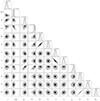 |
Fig. A.1. Corner plot of the perturbed parameters analyzed with Monte Carlo algorithm for system LMC25304 |
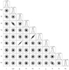 |
Fig. A.2. Corner plot of the perturbed parameters analyzed with Monte Carlo algorithm for system LMC29293. The model satisfies the observations assuming a circular orbit, which means e=0. Therefore, we fixed e and was not included in the MC calculations. |
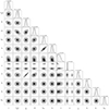 |
Fig. A.3. Corner plot of the perturbed parameters analyzed with Monte Carlo algorithm for system LMC554. |
Appendix B: Comparison with MIST isochrones.
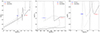 |
Fig. B.1. Mass vs luminosity, effective temperature, and radius diagrams. The solid line is the main metallicity of the system, and dashed lines represent the lower and upper limits of the determined metallicity for system LMC29293. |
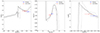 |
Fig. B.2. Same as Figure B.1 but for system LMC25304. |
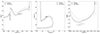 |
Fig. B.3. Same as Figure B.1 but for system LMC554. |
All Tables
Orbital and photometric parameters from the adopted solution using the codes WD and JKTEBOP.
All Figures
|
Fig. 1. Location of our targets (red dots) in the projection of the Large Magellanic Cloud. The blue dots correspond to the systems studied by Graczyk et al. (2018). The underlying image was obtained by The All Sky Automated Survey and originates from Udalski et al. (2008). |
| In the text | |
|
Fig. 2. 6080–6200 Å spectral region of the object LMC25304. The red lines are the disentangled spectra from MIKE-red observations. The black lines are the synthetic spectra generated using the GSSP binary mode. |
| In the text | |
|
Fig. 3. Radial velocity data and their binary solution (upper panel), and the photometric light curve with its solution (lower panel) obtained with the WD code for system LMC29293. The smaller lower panel shows the residuals of our adopted solutions. |
| In the text | |
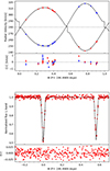 |
Fig. 4. Same as Fig. 3, but for the binary LMC25304. |
| In the text | |
|
Fig. 5. Results of the periodicity search in the light residuals of LMC25304. The upper panel shows the PDM diagram, and the lower panel shows the Lomb-Scargle periodogram. |
| In the text | |
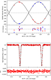 |
Fig. 6. Same as Fig. 3, but for the binary LMC554. |
| In the text | |
|
Fig. 7. Determination of the age for system LMC29293 with theoretical isochrones (black lines). The dashed gray lines correspond to ±1σ uncertainty limits for the metallicity from Table 8. The blue and red crosses mark the masses and luminosities of the primary and secondary components, respectively. |
| In the text | |
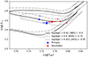 |
Fig. 8. Same as Figure 7, but for system LMC25304. |
| In the text | |
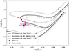 |
Fig. 9. Same as Figure 7, but for system LMC554. |
| In the text | |
|
Fig. A.1. Corner plot of the perturbed parameters analyzed with Monte Carlo algorithm for system LMC25304 |
| In the text | |
|
Fig. A.2. Corner plot of the perturbed parameters analyzed with Monte Carlo algorithm for system LMC29293. The model satisfies the observations assuming a circular orbit, which means e=0. Therefore, we fixed e and was not included in the MC calculations. |
| In the text | |
|
Fig. A.3. Corner plot of the perturbed parameters analyzed with Monte Carlo algorithm for system LMC554. |
| In the text | |
|
Fig. B.1. Mass vs luminosity, effective temperature, and radius diagrams. The solid line is the main metallicity of the system, and dashed lines represent the lower and upper limits of the determined metallicity for system LMC29293. |
| In the text | |
|
Fig. B.2. Same as Figure B.1 but for system LMC25304. |
| In the text | |
|
Fig. B.3. Same as Figure B.1 but for system LMC554. |
| In the text | |
Current usage metrics show cumulative count of Article Views (full-text article views including HTML views, PDF and ePub downloads, according to the available data) and Abstracts Views on Vision4Press platform.
Data correspond to usage on the plateform after 2015. The current usage metrics is available 48-96 hours after online publication and is updated daily on week days.
Initial download of the metrics may take a while.