| Issue |
A&A
Volume 694, February 2025
|
|
|---|---|---|
| Article Number | A65 | |
| Number of page(s) | 22 | |
| Section | Stellar atmospheres | |
| DOI | https://doi.org/10.1051/0004-6361/202452065 | |
| Published online | 04 February 2025 | |
Surface brightness-colour relations of dwarf stars from detached eclipsing binaries
II. Extension of the calibrating sample
1
Centrum Astronomiczne im. Mikołaja Kopernika, Polish Academy of Sciences,
Rabiańska 8,
87-100
Toruń,
Poland
2
Centrum Astronomiczne im. Mikołaja Kopernika, Polish Academy of Sciences,
Bartycka 18,
00-716
Warsaw,
Poland
3
Departamento de Astronomía, Universidad de Concepción,
Casilla 160-C,
Concepción,
Chile
4
Ruhr University Bochum, Faculty of Physics and Astronomy, Astronomical Institute (AIRUB),
44780
Bochum,
Germany
5
Universidad Católica del Norte, Instituto de Astronomía,
Avenida Angamos 0610,
Antofagasta,
Chile
6
Instituto de Astrofísica, Departamento de Ciencias Físicas, Facultad de Ciencias Exactas, Universidad Andrés Bello,
Fernández Concha 700,
Las Condes, Santiago,
Chile
7
French-Chilean Laboratory for Astronomy, IRL 3386, CNRS,
Casilla 36-D,
Santiago,
Chile
8
LESIA, Observatoire de Paris, Université PSL, CNRS, Sorbonne Université, Université de Paris,
5 place Jules Janssen,
92195
Meudon,
France
9
Astrophysics Group, Keele University,
Staffordshire
ST5 5BG,
UK
10
Université Côte d’Azur, Observatoire de la Côte d’Azur, CNRS, Laboratoire Lagrange,
Nice,
France
★ Corresponding author; darek@ncac.torun.pl
Received:
30
August
2024
Accepted:
12
December
2024
Aims. Surface brightness-colour relations (SBCRs) are useful tools for predicting the angular diameters of stars. They offer the possibility to calculate precise spectrophotometric distances based on the eclipsing binary method or the Baade–Wesselink method. Double-lined detached eclipsing binary stars (SB2 DEBs), with precisely known trigonometric parallaxes, allow us to calibrate SBCRs with a high level of precision. To improve such calibrations, it is important to supplement the sample of suitable eclipsing binaries with precisely determined physical parameters.
Methods. We selected ten SB2 DEBs within 0.8 kpc of the Sun, which feature components of spectral types ranging from B9 to K3. We analysed their TESS and Kepler K2 space-based photometry simultaneously with the radial velocities derived from HARPS spectra using the Wilson–Devinney code. The disentangled spectra of DEBs were used to derive atmospheric parameters of their components by applying the GSSP code. The direct effective temperatures were also calculated using spectral energy distribution analysis. The O–C diagrams of the minima times were investigated to detect long-term period changes or apsidal motions.
Results. Most of the systems are composed of significantly unequal components, with mass ratios as low as ~0.5. We derived precise masses, radii, and surface temperatures for them, along with their metallicities. The average precision of mass and radii determinations is 0.3% and 1.4%, respectively, for the surface temperature. The spectroscopic and photometric temperatures of the components are usually consistent to within 100 K, but in some systems, the difference is much larger. The components of HD 149946 show the highest difference (up to 400 K), while the atmospheric models favour different surface metallicities. We also provide an updated calibration of the equivalent width of the interstellar sodium D1 line and the reddening E(B–V).
Key words: binaries: eclipsing / binaries: spectroscopic / stars: distances
© The Authors 2025
 Open Access article, published by EDP Sciences, under the terms of the Creative Commons Attribution License (https://creativecommons.org/licenses/by/4.0), which permits unrestricted use, distribution, and reproduction in any medium, provided the original work is properly cited.
This article is published in open access under the Subscribe to Open model. Subscribe to A&A to support open access publication.
1 Introduction
The empirical stellar surface brightness-colour relations (SBCRs) proved to be very useful in establishing the extragalactic distance scale. When the radius of a star is known, an application of an SBCR gives a robust distance (Lacy 1977b). This approach has allowed for precise distance determinations to be made for globular clusters in the Milky Way (e.g. Thompson et al. 2001) and to the Magellanic Clouds (Pietrzyński et al. 2013; Graczyk et al. 2014), using double-lined detached eclipsing binaries (DEBs). Improved calibrations of the SBCR reached recently a precision of 1% in predicting the angular diameters of main sequence stars (e.g. Salsi et al. 2020, 2021) and GK-type giant stars (Gallenne et al. 2019; Pietrzyński et al. 2019). This development resulted in near-geometrical distance determinations to the LMC by Pietrzyński et al. (2019) and to the SMC by Graczyk et al. (2020), who used rare eclipsing binary stars consisting of late-type giant stars. Both measurements provide so-called geometrical anchors of the extragalactic distance ladder (Riess et al. 2019; Breuval et al. 2024).
Interesting issues regarding SBCRs, which are not yet fully resolved are their dependence on the metallicity and the surface gravity. For example, there are some conflicting results concerning the metallicity dependence (Pietrzyński et al. 2019; Mould 2019). The effect of the surface gravity was noted by several authors (e.g. Fouqué & Gieren 1997; Kervella et al. 2004; Groenewegen 2004); however, it was only indirectly addressed as a dependence on the luminosity class, without providing a quantification of log 𝑔. Salsi et al. (2022) investigated these effects using theoretical atmosphere models and constructing theoretical SBCRs. They concluded that both effects are colour dependent and they are significant (i.e. over 1%) only for the coolest stars of M type. The metallicity effect for main sequence stars was presented by Boyajian et al. (2014), although it was derived from a limited sample of stars and only a constant term was given. The influence of both effects on SBCRs will be addressed by the ongoing SPICA/CHARA interferometry project (Mourard et al. 2022; Ligi et al. 2023), which will measure angular diameters for about 1000 stars with high precision.
On the other hand, eclipsing binary stars with known distances offer the unique possibility to directly derive angular diameters of their components. This route allows for an independent determination of SBCRs (e.g. Kruszewski & Semeniuk 1999; Graczyk et al. 2017) and an investigation of the mentioned second order effects. The abundance of very precise Gaia parallaxes (Gaia Collaboration 2016, 2023) combined with superb quality space-borne light curves results in stellar angular diameters determined with sub-percent precision for a steadily growing number of DEBs.
The present work follows on our previous paper (Graczyk et al. 2021). We identified a number of suitable DEBs, which could serve to improve the calibration of SBCRs for spectral types A, F, G, and early K. The main aim is to expand the calibration sample of DEBs through a very precise determination of their geometrical, dynamical, and radiative properties.
Basic data on the eclipsing binary stars studied in the current work.
2 Observations
2.1 Star sample
Table 1 contains the names and basic parameters of ten eclipsing binary stars selected for the present study. All the systems are classified as double-lined spectroscopic binaries (SB2). Because the systems are well-detached and have no strong spot activity (with the exception of CG Scl), we included them in our sample. Three systems have distances larger than 300 pc, but we included them in the sample because their Gaia DR3 parallaxes (Gaia Collaboration 2016, 2023) are precise to within 1–1.5%. The magnitudes given are averages from catalogues listed in the SIM- BAD/Vizier database after removing outliers and they represent the out-of-eclipse brightness of the systems. CG Scl, AW Col and VZ PsA (=HR 8616) were discovered as variable stars during the HIPPARCOS space mission (Perryman et al. 1997), classified as eclipsing binaries and given names in the General Catalogue of Variable Stars (GCVS; Kazarovets et al. 1999, 2006, 2008).
HD 27476 was identified as an eclipsing binary by Justesen & Albrecht (2021) based on their analysis of the short-cadence photometry from Transiting Exoplanet Survey Satellite (TESS; Ricker et al. 2015). TYC 6511-1799-1, HD 159246 and HD 219869 were found as variable stars and then classified as eclipsing binaries during the All Sky Automated Survey (ASAS, Pojmanski 2002, 2003). BD+17 1832 was found to be an eclipsing binary candidate by Wraight et al. (2011) using STEREO observations and then confirmed by Barros et al. (2016) based on analysis of photometry from K2 space mission (Howell et al. 2014). TYC 266-718-1 was identified as an eclipsing binary by Armstrong et al. (2015) who used also K2 data. HD 149946 was found to be an eclipsing binary by Maxted & Hutcheon (2018) based on K2 photometry.
2.2 Photometry
Almost all stars in the sample were observed by the TESS space mission (Ricker et al. 2015) and, in some cases, K2 data from the extension of Kepler space mission (Koch et al. 2010) was also available. In case of HD 159246, only K2 photometry was available. Table C.1 presents the journal of observations used in the present study. Because K2 photometry has a relatively long cadence of 1800 s, it was rectified to account for the phase smearing during eclipses. The iterative procedure is described in Graczyk et al. (2020).
In most cases, we detrended the light curves to remove long-term changes, usually due to instrumental effects, and also short-term changes due to stellar spots. Removing the spot variability in this way still leaves some small systematic residuals in eclipses, provided the variability is relatively small (up to 0.02 mag). When a few minima are used in a light curve analysis, the systematic trends are mostly cancelled out.
2.3 Spectroscopy
For all systems in the sample, we secured high-resolution spectra with the High Accuracy Radial velocity Planet Searcher (HARPS; Mayor et al. 2003) on the European Southern Observatory 3.6-m telescope at La Silla, Chile. We dedicated a number of ESO observing proposals to obtain full radial velocity curves. The ESO observing programs were 0100.D-0339, 0101.D-0697, 0102.D-0281, 105.20L8, 106.20Z1 (PI G. Pietrzyński), 105.2045, 108.21XB (PI D. Graczyk), 099.D-0380 and 0100.D-0273 (PI W. Gieren). In total we collected 129 spectra between 2017 June 10 and 2021 October 26 (see Table C.2). Typical integration times were between 10 and 15 min. Almost all spectra were taken in the highest resolution ECHELLE mode. The spectra were reduced on-site using the HARPS Data Reduction Software (DRS).
In the case of the highly eccentric system TYC 6511-1799-1, for which we collected only nine epochs, our HARPS data was supplemented by literature data. We added 20 radial velocity epochs from Ratajczak et al. (2021). Their velocimetry is of a lower precision than ours, but when both sets of radial velocities are solved independently they provide similar orbital parameters to within errors.
Best-fitting atmospheric parameters, together with their 1σ uncertainties.
3 Analysis of spectra
3.1 Radial velocities
We used the RaveSpan code (Pilecki et al. 2017) to measure the radial velocities of the components in all systems via the broadening function (BF) formalism (Rucinski 1992, 1999). We used templates from the library of synthetic LTE spectra by Coelho et al. (2005) matching the mean values of the estimated effective temperatures and surface gravities of the component stars. The abundances were assumed to be solar.
The secondary’s lines in VZ PsA are barely detectable in the spectra because of the high light ratio of the components, therefore we used a procedure previously applied to V362 Pav (Graczyk et al. 2021). In short, we stacked all spectra of VZ PsA to get the best signal-to-noise ratio (S/N) spectrum of the primary, which was later subtracted from spectra to get the clean BF signal of the secondary. Radial velocity measurements for all systems are summarised in Table C.3.
3.2 Spectral disentangling
The radial velocities derived in Sect. 3.1 were used to decompose the observed spectra of each system into the spectra of the individual components. For disentangling we used all HARPS spectra, with the exception of a few spectra with a very low S/N or with very prominent solar features (when taken at bright evening and morning sky). We used the RaveSpan code which utilises the method presented by González & Levato (2006). We ran two iterations choosing a median value for the normalisation of the spectra. The disentangled spectra cover the spectral range from 4300 Å up to 6900 Å.
3.3 Stellar atmospheric analysis
3.3.1 Methods
The atmospheric parameters of the binary system components were derived using an analogous technique to the one described in our previous papers of the series (Graczyk et al. 2021, 2022). We fit synthetic spectra to the high-resolution (R~80000 and ~ 115 000) HARPS disentangled spectra (Sect. 3.2) with the use of the binary version (August 2020) of the ‘Grid Search in Stellar Parameters’ (GSSP) software package (Tkachenko 2015). The code employs the spectrum synthesis method by using the SYNTHV LTE-based radiative transfer code (Tsymbal 1996). The GSSP code provides two grids of atmosphere models: the LLMODELS grid (Shulyak et al. 2004) for hotter (Teff > 5500 K) stars and the MARCS (Gustafsson et al. 2008) models useful here in a few cases of systems containing cooler secondary components (CGScl, TYC266-718-1, and TYC 1257-132-1). The GSSP_binary version uses the spectra that are not corrected for a companion’s flux (the dilution). Instead, a flux ratio, ƒi, is calculated by the GSSP code utilising a ratio of the components radii (r1/r2) from a solution derived with the Wilson-Devinney programme (see Table C.4). The macroturbulent velocity (ζ) parameter, which strongly correlates with the rotational velocity (Vrot), cannot be calculated as a free parameter; thus, its value was estimated using published relations (Smalley 2014; Gray 2005) and fixed during the calculations (Table 2).
In general, we used four free parameters: metallicity ([M/H]), effective temperature (Teff), microturbulent velocity (ξ), and Vrot sin i. The GSSP code calculates synthetic spectra for each set of grid parameters and compares them with the normalised decomposed spectrum. The χ2 value is calculated for each pair to judge the goodness of fit and to choose the best-matching (corresponding to minimum χ2) values within the grid of synthetic spectra. Additionally, the chemical composition for ~30 elements was calculated for all objects from the current sample. The detailed abundance analysis of the atmospheres of these stars will be published separately (Gałan et al., in prep.). In most of the systems at least one of the components shows overabundance of lithium. Several systems contain components that show characteristics of Am-type stars – with strongly enhanced barium, yttrium, zirconium, strontium, and zinc, and deficient in calcium and/or scandium.
The regions around the Hα, Hβ, and Ηγ lines were excluded from the analysis. Except for VZPsA, the spectrum beyond Ηγ was also excluded because of a significantly lower S/N. Additionally, a number of narrow spectral ranges was excluded from the analysis with the use of a self-developed program that generates two kinds of individual masks, to eliminate wrong or noisy areas. The first mask removes noisy ranges with no spectral lines deeper than 2.5 σ of the noise. The second mask eliminates the features in the decomposed spectra that have no counterparts in the line lists, as well as those cases in the synthetic spectra that have bad data for atomic transitions. Also, the regions containing artefacts from imperfectly removed features from atmospheric lines of water (H2O: mainly λ ~ 5880–6000 Å) and dioxygen (O2: λ ~ 6274–6330 Å) were skipped.
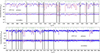 |
Fig. 1 5054 – 5257 Å (top) and 5608–5884 Å (bottom) regions of disentangled spectra of the primary and the secondary components of AW Col with selected spectral lines identified. Strong lines from ionised yttrium (Y II λ 5087.42, 5200.41, 5205.72, and 5662.92 Å), and barium (Ba II λ 5853.67 Å) are visible. The red lines denote the atmosphere model fits to the observed spectra (blue). The gray shaded areas were excluded from calculations by the use of an individual mask. |
3.3.2 Atmospheric parameters
The input values for the parameters were based generally on the results of modelling with the Wilson-Devinney (hereafter WD) code (see Sect. 5; Tables C.4 and 5). In particular, the surface gravity (log 𝑔) was fixed to the values from the WD solution. We searched initially around the solar value for metallicity [M/H]. The input values for the micro-turbulent velocity (ξ) were estimated using published correlations with log 𝑔, and spectral types or Teff (Gray et al. 2001; Gray 2005; Smalley 2014; Sheminova 2019), and according to Landstreet et al. (2009) for hotter stars (Teff ≳ 8000 K). In two cases where the faint secondaries of HD 27476 and VZ PsA contribute very little to the total flux of the systems and where the disentangled spectra show very low S/N, it was not possible to determine the ξ parameter from the spectra. Instead ξ was set based on the Gaia-ESO iDR6 calibration (R. Smiljanic, 2021, private communication) according to their Teff and [M/H] (see Table 2).
The procedure of solution was nearly identical to what has been used recently (Graczyk et al. 2022). We started the analysis using coarse but wide grids of parameters to find the region approaching the global minimum. In the next steps, the parameter ranges were narrowed step by step, making the sampling finer. The parameters of the best-matching models corresponding to the requested atmospheric parameters were found in several iterations. The 1σ uncertainties were estimated by finding the intersection of the 1σ levels in χ2  with the polynomial functions that have been fitted to the minimum values of reduced χ2 as recommended by Tkachenko (2015). The resulting final parameters are shown in Table 2. The samples of decomposed spectra in two spectral regions for AW Col are compared with the best fit synthetic spectra in Fig. 1.
The metallicities of the stars in the sample are distributed around the solar value. Two systems are characterised by [M/H] ~−0.4 dex, while there are three cases with super-solar metallicities up to [M/H] ~ +0.6 dex in the systems containing Am-type stars (see Table 2).
The stars in our sample rotate mostly with nearly synchronous (Vrot sin i) velocities to within a 3σ error. The most striking exceptions are the primary component of AW Col, which rotates much faster, and VZ PsA, which rotates more slowly.
Reddening determinations.
4 Effective temperature determination
4.1 Interstellar extinction
4.1.1 3D map
We used the three-dimensional (3D) interstellar extinction map STILISM (Capitanio et al. 2017), which provides all-sky reddenings up to a distance of ~2 kpc from the Sun. The distance depth of the map strongly depends on the galactic latitude, which is largest near the galactic equator and decreases to ~300 pc near the galactic poles. The distances to our targets were calculated as the inverse of the parallaxes given in Table 1. As an uncertainty, we adopted one-third of the maximum uncertainty returned by the extinction map at the given distance, that way E(B – V) based on the map have similar weights to extinctions derived from Na I in the following section. The reddenings are listed in Table 3.
4.1.2 Sodium lines
The interstellar sodium doublet Na I (5889.951, 5895.924 Å) is widely recognized as a good tracer of interstellar extinction (e.g. Munari & Zwitter 1997, and references therein). Calibrations between the colour excess E(B– V) and the equivalent width of Na I lines based on high-resolution spectroscopy were published by a number of authors and more recently by Poznanski et al. (2012). In that paper, the authors claimed a systematic difference between their calibration based on extragalactic SDSS/QSO data and the results of Munari & Zwitter (1997) from spectroscopy of galactic OB stars. We believe this difference arises only from a comparison of the data of Poznanski et al. to the relation given by Eqs. (2) and (3) in Munari & Zwitter (1997). When the data from both papers are compared to each other directly, there is no systematic offset (see Fig. 2). We obtain a simple relation between the equivalent width EW of the Na I D1 line and E(B – V), using original data from both papers for EW < 0.35 Å:
 (1)
(1)
The above relation is valid for the EW of a single Na I component smaller than 0.35 Å, and its precision is about 10% while accuracy is better than 0.02 mag in predicting the reddening. It is out of the scope of the present paper to discuss the intriguing systematic deviations from the relation given by Eq. (1), but their presence clearly indicates a need for an independent recalibration of this useful relation. The possible systematic effects affecting measurements and calibration of the sodium line relation, potentially leading to some observed deviations are discussed in Sect. 5.1 and the appendix of Poznanski et al. (2012).
Using the HARPS spectra with the resolving power of ~100 000, we determined the sodium line EWs for nine systems in our sample. The exception is CG Scl, for which we could not identify any interstellar component of Na I, most probably because of the proximity of the system. The most complex shape of the interstellar sodium doublet is present in HD 159246, which has at least seven different components, and is the most reddened system in the sample. In the majority of systems, however, only one or two components are visible, as reddenings are low in their directions. By utilizing Eq. (1), we were able to determine the interstellar extinction E(B – V), with the results are reported in Table 3.
The agreement with the STILISM map is good, on average; however, in the case of the two most reddened systems (HD 149946 and HD 159246), the differences are larger than 2σ. Finally, we calculated the weighted means from both methods; with the exception of HD 149946, for which we used an ordinary mean. The adopted values of E(B – V) are listed in the last column of Table 3. These were used in all following parts of the analysis, especially for the derivation of the radiative parameters of the stars.
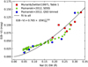 |
Fig. 2 Relation between the equivalent width of the sodium line D1 and the reddening. |
4.2 SED reconstruction
We used a direct approach for measuring the effective temperatures of stars in detached eclipsing binary systems, first described by Miller et al. (2020). For a DEB with parallax ϖ, the extinction-corrected flux observed at the top of the Earth’s atmosphere is
![${f_{0,b}} = {f_{0,1}} + {f_{0,2}} = {{{\sigma _{{\rm{SB}}}}} \over 4}\left[ {\theta _1^2{\rm{T}}_{{\rm{eff}},1}^4 + \theta _2^2{\rm{T}}_{{\rm{eff}},2}^4} \right],$](/articles/aa/full_html/2025/02/aa52065-24/aa52065-24-eq3.png)
where σSB is the Stefan-Boltzmann constant, and the angular diameter θ for each star can be expressed as θ1,2= 2R1,2 ϖ. These parameters are known for the DEBs in this work, or can be measured if we can accurately integrate the total stellar flux for each star independently. The method uses EMCEE (Foreman-Mackey et al. 2013) to sample the posterior probability distribution P(Θ|D) ∝ P(D|Θ)P(Θ), which has model parameters Θ and prior P(Θ), given the data, D (observed magnitudes and light ratios). The model parameters are the effective temperatures Teff,1,2 and angular diameters θ1,2 for each component, the colour excess E(B – V), the hyper-parameters σext, σℓ which account for additional uncertainties in the synthetic magnitudes and light ratios respectively, and N distortion polynomial coefficients for each star c1,N, c2,N. In this work, we let N equal 2 when the observed light ratio in available only in one photometric band, or 3 when it is available in two. The observed magnitudes used in the analysis are sourced from Gaia EDR3 (Gaia Collaboration 2021), the 2MASS survey (Skrutskie et al. 2006) and the WISE All-Sky Release Catalog (Cutri et al. 2012) with corrections to Vega magnitudes from Jarrett et al. (2011). Ultraviolet magnitudes from GALEX (Martin et al. 2005) and u, v magnitudes from SkyMapper DR4 (Onken et al. 2024) were used whenever available. Full details of the photometric zero-points and response functions used to calculate synthetic magnitudes in these bands are given by Miller et al. (2020). Gaussian priors were placed on reddening (see Sect. 4.1), angular diameters (calculated from the stellar radii derived in Sect. 5.4 and Gaia trigonometric parallaxes), and the flux ratio in the near-infrared (based on colour-Teff relations which were calculated for each star using the approach described in Miller et al. 2020). To calculate the bolometric flux and hence the effective temperature for each component, we construct a flux integrating function for each star by multiplying a model SED (calculated from BT-Settl model atmospheres; Allard et al. 2013) with a distortion function, which is a linear superposition of Legendre polynomials. The distorted SED for each star is then normalised, such that the total apparent flux before reddening is  . These resulting functions can then be used to calculate synthetic photometry, taking into account realistic stellar absorption features, while noting that the overall shape of the function can be adjusted to match the observed data. This means that the effective temperatures derived using this method are based on the integrated stellar flux and angular diameter, rather than traditional SED fitting.
The method has been demonstrated to produce the most reliable results when using a number of light ratios in different bands to better constrain each star’s contributions to the total flux (Miller et al. 2020). In our sample, six systems have a light ratio determined only in one band (TESS or Kepler) while four systems have two light ratios. Additionally, four systems contain relatively hot components with surface temperatures of about 10 000 K. In order to derive precise temperatures for these systems, reliable ultraviolet fluxes and light ratios in the blue are necessary. Thus for the purpose of this work, we omitted the four hottest systems in this section of the analysis. The results for the remaining systems are given as TSED in Table 4.
Effective temperature determinations.
4.3 Colour-temperature calibrations
To estimate the Teff values of individual components, we collected multi-band magnitudes of the systems. We used 2MASS (Cutri et al. 2003) for the near-infrared photometry and converted the magnitudes into Johnson photometric systems using transformation equations from Bessell & Brett (1988) and Carpenter (2001). To determine the intrinsic colours of the components, we applied the reddenings derived in Sect. 4.1 and the extrapolated near-infrared light ratios from the Wilson–Devinney code (Sect. 5).
We determined Teff values from a number of colourtemperature calibrations for a few colours: B – V (Alonso et al. 1996; Flower 1996; Ramírez & Meléndez 2005; González Hernández & Bonifacio 2009; Casagrande et al. 2010), V – J, V – H (Ramírez & Meléndez 2005; González Hernández & Bonifacio 2009; Casagrande et al. 2010), and V – K (Alonso et al. 1996; Houdashelt et al. 2000; Ramírez & Meléndez 2005; Masana et al. 2006; González Hernández & Bonifacio 2009; Casagrande et al. 2010; Worthey & Lee 2011). For the few calibrations having metallicity terms, we assumed the metallicity derived from the atmospheric analysis (see Table 2). The resulting temperatures were averaged for each component and are reported in Table 4 in column Tcol. The errors reported are standard deviations of a sample of all temperatures derived for a given component; however, we fixed a minimum uncertainty to 1%of Tcol.
4.4 Final adopted values
The precise determination of the effective temperatures Teff is important because we do not adjust limb darkening coefficients whilst fitting the light curves. Instead, these coefficients are calculated for a given set of surface atmospheric parameters (Teff, log 𝑔) using tables from van Hamme (1993). Surface gravities are well determined internally within the Wilson–Devinney code, but to determine Teff we need external information.
We derived Teff in three ways: spectroscopic temperatures Tspec (Sect. 3.3.2) and two photometric temperatures TSED (Sect. 4.2) and Tcol (Sect. 4.3). They are all reported in Table 4, where we assume a minimum uncertainty of 50 K for Tspec. Combining spectroscopic and photometric temperatures is not trivial because they do not share the same systematic uncertainties. In general the mutual agreement between them is satisfactory, although in some cases differences are larger than 200 K. One can notice, however, some systematic effects e.g. Tspec is on average larger than TSED and Tcol by about 100 K. For six systems for which we have all three temperature determinations weighted average differences are Tspec − TSED = 86 K and TSED − Tcol = 28 K. The difference between spectroscopic and photometric temperatures reflects to some extend the choice of atmospheric models.
The preferred approach would be the direct method based on the SED reconstruction (Sect. 4.2), however, because of the small number of available light ratios per system, we did not choose it. Instead, we combined the surface temperatures in two ways. In the first approach, we simply calculated the weighted means separately for both components which are listed in Table 4, in column Tmean. The second method implements an additional constraint which is the temperature ratio T21 = T2/T1 provided by models. The temperatures are calculated according to the equations:
 (2)
(2)
 (3)
(3)
 (4)
(4)
where L21 are the model light ratios from Table C.4. The calculated temperatures, T1,2, are listed in Table 4 as Tadopted. Usually, there is a very good agreement seen between temperatures calculated with the two methods above. However, in cases of much fainter and cooler secondaries, these temperatures are significantly different. We prefer the second method because the resulting temperatures are in full agreement with light ratios provided by the WD models. This is especially important for an extrapolation of light ratios in different photometric bands, particularly in the near-infrared.
5 Analysis of light and radial velocity curves
For the analysis of the eclipsing binaries, we made use of the Wilson-Devinney program (WD) version 2007 (Wilson & Devinney 1971; Wilson 1979, 1990; van Hamme & Wilson 2007)1, equipped with a Python wrapper and a newer version of the WD code (Wilson & Van Hamme 2014, LCDC2015, version 2019), directly includes the TESS bandpass2. We used a specific python GUI3 written for this newer version of the WD code (Güzel & Özdarcan 2020, PyWD2015).
5.1 O–C analysis
We constructed the O–C diagrams for all systems, with the exception of HD 159246, for which there is only a relatively short set of photometric measurements from K2 (Campaign 11). We set ourselves several objectives: 1) a precise determination of the orbital ephemeris; 2) detection of a possible light-time-effect (LTE) due to an unresolved companion; and 3) detection of apsidal motion in eccentric systems. For the apsidal motion analysis, we used the equations given in Giménez & Bastero (1995).
We calculated minima times from public K2 and TESS photometry and in the case of CG Scl also from Super-WASP observations (Pollacco et al. 2006). For CG Scl, AW Col, TYC 6511-1799-1 we augmented this data with minima times from the TIDAK database (Kreiner 2004; Kim et al. 2018). Additionally, we also used minima times from the literature (Otero & Wils 2005; Maxted & Hutcheon 2018). The resulting O-C diagrams are presented on Fig. B.1.
The derived orbital periods were then fixed during the simultaneous analysis of photometry and velocimetry with the WD code. None of the nine investigated EBs shows any trace of period changes. Out of eight investigated eccentric systems we could detect an apsidal motion in three cases: AW Col, TYC 6511-1799-1, and VZ PsA. These three EBs show a slow periastron advancement with the apsidal motion period U of tens of thousands of years.
5.2 Initial parameters for the WD
In the first step we fixed Teff of the primary component during the analysis to the average of the Teff values derived from the colour–temperature calibrations Tcol and the atmospheric analysis Tspec. The procedure is iterative: we derived preliminary model parameters with the WD code assuming the best guess initial temperature T1 from colour-temperature calibrations. The derived ratio of the radii was used in the atmospheric analysis to derive Tspec. Then we calculated new models with updated temperatures, which were used later to redetermine the photometric temperatures TSED and Tcol.
The standard albedo and gravity brightening exponent for radiative and convective stellar atmospheres were adopted assuming the conversion temperature of T = 7200 K. However in many cases we fitted the albedo parameter to one or both components. The stellar atmosphere option was used (IFATl=IFAT2=1), radial velocity tidal corrections were applied (ICORl=ICOR2=1) and no flux-level-dependent weighting was used. We assumed synchronous rotation for both components in all systems (F1=F2=1) with an exception of fast rotating components of AW Col (F1=5, F2=3) and HD 149946 (F1=F2=3). The logarithmic (Klinglesmith & Sobieski 1970) limb-darkening law was used (LD1=LD2=−2), with coefficients precomputed and tabulated for specific bands van Hamme (1993). We assumed a detached configuration in all models (mode 2 of the WD code) and a simple reflection treatment (MREF=1, NREF=1).
5.3 Fitting the model parameters
With the WD binary star model we fitted simultaneously light curves and radial velocity curves of both components using the grid fineness parameters N1=N2=80. In cases in which one of the stars was significantly larger than its companion, it was necessary to use a higher numerical precision and we set N=100 for the larger star. Each observable curve was weighted only by its rms through comparison with the calculated model curve. We adjusted the following parameters during the analysis: the orbital period, Porb, the epoch of the primary eclipse, T0 in cases of circular orbits, the phase shift, ф, when orbits were eccentric, the semimajor axis, a, the mass ratio, q, the systemic radial velocity, γ, the eccentricity, e, the argument of periastron, ω, the orbital inclination, i, the temperature of the secondary, T2, the modified Roche potentials, Ω1,2 (corresponding to the fractional radii r1,2 = R1,2/a ), and the luminosity parameter, L1. Additionally, we made a fitting for a third light, ℓ3. The best models were chosen according to their reduced χ2 and a lack of significant systematic trends in the residuals.
The statistical (formal) errors on the fitted parameters were estimated with the Differential Correction sub-routine of the WD code. We assumed conservative errors on parameters: we multiplied the formal errors by a factor of 2. The model synthetic light curves compared to photometric observations are presented in Fig. B.2 for all ten systems. The radial velocity solutions plotted against measured velocities are presented in Fig. B.3.
The best-fit model parameters for all systems are summarized in Table C.4. The systemic velocity is not corrected for the gravitational redshift or convective blueshift. The absolute dimensions of the systems were calculated using nominal astrophysical constants advocated by the IAU 2015 Resolution B3 (Prša et al. 2016) and are presented in Table 5. The metallic- ities are weighted mean values for both components with the exception of HD 149946.
Physical parameters of the eclipsing binary stars.
5.4 Analysis details and results
5.4.1 CG Scl
In order to build a model of this system we used photometric time series from three TESS sectors and a set of 14 HARPS spectra. CG Scl consists of two late type, unequal main sequence stars forming a well detached system on a slightly eccentric orbit. Both eclipses are total. Their metallicity is solar and both rotate synchronously. The more massive, larger and hotter primary, seems to be a little inflated due to stellar evolution. This is the lowest mass system in the sample.
Light curves from all three TESS sectors show quite significant spot activity, inferred from out-of-eclipse variations. The variations are sinusoidal, have a semi-period between 12.5– 13.5 d, depending on the sector, and the light curve modulation has an amplitude of ~0.02 mag. The period of the light curve modulation is a bit longer than the orbital period that suggests that spots drift on the surface. Both components host the spots as systematic residuals are visible in both eclipses. The primary is probably the more spotted, active one. The spot activity of CG Scl is by far the largest in the present sample. The system is also a weak X-ray source discovered by the ROSAT all-sky survey (Metanomski et al. 1998).
For the purpose of analysis with the WD code the out- of-eclipse light curve modulation was removed using splines. Although the final light curve solution is very good, residuals in eclipses show systematic trends due to the spot presence which reach 2500 ppm in Sector 2 and 4000 ppm in Sectors 29 and 69. The radial velocity solution has no clear systematic trends and the RV curves have rms values of 57 m s−1 and 73 m s−1 for the primary and the secondary, respectively. The rms for the primary is much larger than the typical RV measurement error (18 m s−1) which is caused by the presence of spots.
The masses, temperatures, and intrinsic colours of the components correspond to spectral types G2V and K3V. Houk (1982) listed two alternate spectral types G5V (composite?) and F/G + G8/K0 which agrees quite well with our classification. Interestingly CG Scl shows a significant proper motion anomaly (Kervella et al. 2022), which may signify the presence of a tertiary companion affecting its motion. However, the O–C analysis (Sect. 5.1) did not reveal period changes nor an apsidal motion (Fig. B.1), although minima times cover 22 years. A face-on orbit of the tertiary would explain the proper motion anomaly and a lack of the LTE.
5.4.2 HD 27476
This eclipsing binary is in fact a wide triple system, because it forms a common proper motion pair with the nearby 18th mag star, Gaia DR3 4782816310277777792. The colours and observed brightness of the tertiary companion are consistent with a M2.5 red dwarf. The separation is 15 arcsecs, which corresponds to a projected distance of about 5000 AU.
The main binary consists of two unequal, main sequence stars. The hotter and more massive primary is a metallic line Am star with significantly strengthened s-elements and strong lines of Sr and Zn. The much cooler secondary has an overabundance (~2 dex) of lithium and contributes only 9% to the total flux in the TESS band and 5% in the V-band. The orbit is slightly eccentric and the secondary eclipse is total.
The TESS light curves show very small out-of-eclipse sinusoidal variations due to spots with a period of ~7.2 days. We did not detrend the light curves, instead we choose the TESS Sectors 30 and 32 during which the minimum/maximum of the out-of-eclipse changes approximately overlap with the pri- mary/secondary eclipse. This way we could fit the light curves by adjusting the albedo parameter without the need to insert small, cool spots on the stellar surface. The light curves from Sectors 03–05 are more asymmetric with respect to the eclipses and we decided to not use them in the analysis. The resulting albedos are A1 = 1.0 and A2 = 0.68 in good agreement with expected values.
The light curve solution is of very good quality. There are no systematic deviations within the primary eclipse, while within the secondary eclipse very small systematic residuals reach about 250 ppm. The radial velocity solution has no systematic trends and the RV curves have rms values of 230 m s−1 and 320 m s−1 for the primary and the secondary, respectively.
The spectral type given by Houk (1978) is A0V while the temperature and the intrinsic colours of the primary correspond to B9.5V. The surface parameters of the much fainter companion correspond to F8V. We adopted an A0mV+F8V system.
5.4.3 AW Col
The system consists of two different main sequence stars orbiting on a highly eccentric orbit. Both eclipses are total and they resemble in shape and depth eclipses of CG Scl. Light curves from both TESS sectors show a small spot modulation with a semi-period of 7.6 days. Interestingly the best fit to the detrended TESS light curve shows only a slight increase of residuals during the primary eclipse, while during the secondary eclipse residuals are significant and they change between two sectors. This means that practically all spots lay on the secondary component whose flux varies by up to 3% due to the spots.
With the O–C diagram analysis we detected a slow rate of periastron advance of  rad cycle−1 (see Fig. B.1), which corresponds to the apsidal motion with a period of about U ≈ 16000 yr. The
  was later fixed during analysis with the WD code.
In total, we collected 13 HARPS spectra; however two spectra were taken closely to spectroscopic conjuction and the lines of both components were heavily blended. We were able to unequivocally derive the radial velocity of the secondary from only one of these spectra. Another spectrum was taken during the primary eclipse that affected RV determination. Therefore, we dropped this RV of the primary from the analysis. The rms values of solution are 69 m s−1 and 170 m s−1 for the primary and the secondary, respectively.
The hotter and larger primary dominates the spectrum. Houk (1982) reports a spectral type of a single metallic-line star: A3m:A7-A7. We also detected that the primary is a weak metallic-line star. It has stronger lines of Br, Zn and Sr and some underabundance of Ca and Sc. This is interesting, because both components rotate much faster than the synchronous rotation, although a bit slower than the pseudo-synchronous rotation. Similarly to HD 27476 the secondary shows some enhancement of Li. Based on spectral features, temperatures and intrinsic colours we estimate spectral type of the system as A7mV+G2V.
5.4.4 TYC 6511-1799-1
The system consists of two similar, slightly evolved stars. The components have marginally sub-solar metallicity and both have an enhancement of lithium. The orbit is strongly eccentric and both eclipses are deep and partial. During the deeper, primary eclipse a slightly smaller, cooler and less massive component is eclipsed. Because of the eccentricity, the secondary eclipse is almost three times longer than the primary. The out-of-eclipse TESS light curve is practically flat and there is only a very small modulation with an amplitude of about 0.0005 mag.
The system shows a slow apsidal motion with a rate of  rad cycle−1 (Fig. B.1), which corresponds to a period of U ≈ 37 000 years. The derived rate of the periastron advance was fixed during analysis with the WD code.
The best solution has no systematic residuals in the eclipses. The radial velocity solution has quite large residuals with the rms of 290 m s−1 and 240 m s−1 for the primary and the secondary, respectively. This system is the faintest in our sample and most of its HARPS spectra have low S/N. The precision of the individual RV measurements is about 55 m s−1. The large rms is caused mainly by the use of less precise RVs from Ratajczak et al. (2021). The rms of RVs derived from HARPS spectra alone are 90 m s−1 and 29 m s−1 . Both components rotate faster than the synchronous rotation but much slower if periastron tidal synchronization would occur. The spectral type of the system estimated from surface temperatures and gravities is F8IV+F7IV.
5.4.5 BD+17 1832
This binary has a circular orbit and consists of two notably different main sequence stars. Both eclipses are partial, the primary is the larger, hotter and more massive star. Obtaining a consistent, simultaneous solution to the velocimetry and K2 data together with TESS data was difficult because the temperature ratio from TESS data alone was 0.887(1) while from K2 data it was 0.895(1). All simultaneous solutions showed large K2 data residuals during eclipses. When K2 and TESS photometry was fitted separately we could find good models with mutually consistent geometric parameters including the orbital inclination and radii. Separate solutions did not show any significant systematic residuals in the eclipses.
The spectroscopic temperature ratio from the GSSP analysis (Sect. 3.3) is 0.924(19) i.e. about 2σ larger than the photometric temperature ratios. On the other hand both components have solar metallicity and taking into account the relatively low mass and radius of the secondary, the higher temperature ratio is quite unlikely. For this reason, we adopted the one obtained with TESS data alone as our solution.
Both components seem to rotate synchronously. The primary has an easily visible enhancement of s-processed elements (both light and heavy). The spectral type of the system estimated from LAMOST spectra is A3IV (Qian et al. 2018) in agreement with our estimate of A3V+F0V. The radial velocity solution does not show any systematic deviation. The rms of the solution is 33 m s−1 for the primary and 200 m s−1 for the secondary.
5.4.6 TYC 266-718-1
This binary contains two main sequence stars, which are only slightly more massive than the components of CG Scl. The primary is much brighter than its companion. The system has the longest orbital period in the sample, which results in a large relative separation of the components; the sum of fractional radii is: r1 + r2 = 0.035. Despite this, the eclipses are total, because the orbital inclination is very close to 90 degrees. The out-of-eclipse parts of the light curves do not show any significant modulations due to spots or pulsations.
In the beginning, we tried to find a simultaneous fit to the TESS and the K2 data. However, it turned out that the K2 light curve shows relatively large systematic residuals during the eclipses, especially within the secondary eclipse. Also, including K2 data produces large systematic residuals in the radial velocity solution. With the O–C diagram analysis we checked that the system did not show an apsidal motion or period changes (see Fig. B.1). Thus we assumed that the orbital period is constant.
We fit the K2 data separately to investigate the source of residuals. The solution from the K2 data shows much smaller residuals and has very similar parameters to the solution found with TESS data alone, with two exceptions: the temperature ratio and the eccentricity. From the TESS data T2/T1 = 0.8711(2) and from the K2 data T2/T1 = 0.8743(1), while e = 0.0487(2) and e = 0.0502(2), respectively. The lower eccentricity fits radial velocity curves much better, therefore we decided to keep only the TESS data in the final simultaneous solution.
The system has solar metallicity; however, in this case, it is the hotter primary, which is enriched in lithium, while no Li line can be detected in the secondary. The spectral type derived from LAMOST spectra is G0 (Hardegree-Ullman et al. 2020) in agreeement with our estimate G0V+K0V based on the surface temperatures and gravities. The components rotate very slowly, in a seemingly synchronous rotation despite the large separation between them. The radial velocity solution has the smallest rms in the sample: 29 m s−1 and 44 m s−1, for the primary and the secondary, respectively.
5.4.7 HD 149946
This system has a slightly eccentric orbit and its components differ in size and mass, but have very similar surface temperatures. The eclipses are partial and relatively shallow. For the O–C analysis we included additionally minima times derived from TESS long-cadence data from Sector 12. Figure B.1 shows the O–C diagram for the system. We did not detect any significant period changes nor apsidal motion.
The best-fit simultaneous solution to the TESS and K2 light curves still shows residuals reaching up to 1000 ppm in eclipses. However solutions found using the TESS and the K2 light curves alone show no systematics. The situation is similar to that encountered in TYC 266-718-1, however systematic residuals are not so large. To solve the tension we employed the linear limb-darkening law (LD1=LD2=+1) and we fitted four linear coefficients – in two bands for each component. We kept the same system’s geometry like in the best-fit solution found with the logarithmic LD law. With this approach we obtained significantly lower  and systematic residuals were reduced to about 400 ppm and 800 ppm in the primary and the secondary eclipse, respectively. The linear coefficients are x1 = 0.478(6) and x2 = 480(12) in Kepler band and x1 = 0.409(7) and x2 = 430(12) in TESS band. That solution was adopted as the final one. However, it must be noted that separate fits to K2 and TESS light curves done with our standard procedure (i.e. LD1=LD2=−2) give slightly lower the rms.
Finding consistent radiative parameters for this system proved difficult. The unconstrained GSSP solution to disentangled spectra favours components with significantly different surface metallicities (at 4σ) and high effective temperatures of about 6650 K (see Table 2). We calculated an additional solution setting the metallicity of the secondary to be equal to the primary’s metallicity from the unconstrained solution. This solution has a lower [M/H] ~ −0.6 dex for the primary and lower surface temperatures by about 350 K – see the second line for HD 149946 in Table 2. It is formally a slightly worse fit than for the metallicity set as an entirely free parameter, yet the effective temperatures are in better agreement with results from the SED analysis and the colour-temperature calibrations (see Table 4). We also tested a solution forcing the same surface metallicity for both components. The best fit returns [M/H] ~ −0.7 dex and even lower temperatures by 100 K but it is disfavoured because of larger residuals in lines of individual elements.
The higher temperature values in the range of 6600–6700 K are supported by the spectral type F3V determined by the Michigan Spectral Survey (Houk 1982), and the mass of the primary component (1.42 M⊙) which on the main sequence would correspond to the spectral type F3. Finally, we adopted average temperatures, which lie in between the best spectroscopic and photometric temperatures, but we assigned large errors to them, which reflect a lack of consistency. HD 149946 is the only system listed in Table 5 with no mean metallicity given in accordance with the GSSP results. The best-fit light curve solution indicates that the primary component is slightly inflated suggesting a somewhat later spectral type than F3. Indeed our best estimate of spectral types based on effective temperatures and log ɡ is F5IV+F6V.
Both components rotate by a factor of 2.5 faster than synchronous or pseudo-synchronous rotation. The stars are well separated, the sum of their relative radii r1 + r2 is only 0.0726. The rms of the radial velocity solution is 67 m s−1 and 135 m s−1 for the primary and the secondary, respectively.
5.4.8 HD 159246
This is the most massive system is our sample. It consists of two very similar late B-type metallic stars orbiting on a circular orbit. The eclipses are deep, central and almost of equal depth. This is the only system which has no TESS light curve. Therefore the light curve analysis was based on rectified K2 data. The light curve shows considerable out-of-eclipse modulation with an amplitude of 0.003 mag. The modulation is symmetric with respect to eclipses.
To reproduce the magnitude of the modulation we tested two models: a) one fixed, cool spot on each component opposite to each other and b) adjusting the albedo parameter A1,2 for both components. The better overall fit can be achieved with model a), especially as the shape and the magnitude of modulations is fairly well reproduced. In the case of model b), even for A1 = A2 = 0 we could not reproduce the amplitude. Only by assumption of unphysical negative albedos it was possible to obtain proper modulation. Finally, we adopted the model with spots. The resulting spots are similar to each other, the ratio of the spots temperature to the mean surface temperature is 0.95 and the angular radius of the spots is 0.17 rad.
Within the eclipses, the residuals are larger by a factor of three than in out-of-eclipse parts of the light curve. The depth of the eclipses is slightly and erratically changing with different epochs. This could be caused by cool spots changing their position and shape. The third light is small but significant: ℓ3 = 0.033 ± 0.001. There is a nearby, red star 2MASS 17342139- 1836134, which is fainter by ~4 mag in the Gaia G-band, which probably affected the K2 photometry. The star is not a physical companion of HD 159246.
Both components rotate synchronously with υ sin i = 23 km s−1. This is a result of the relatively short orbital period and large stellar radii. The radial velocity solution has rms values of 880 m s−1 and 810 m s−1. These are by far the largest rms values in the sample, but they are consistent with the RV measurements errors. There are two main reasons for the large RV errors: the stellar lines of HD 159246 are considerably broadened by the rotation and the HARPS spectra have relatively low S/N for such early-type stars.
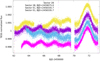 |
Fig. 3 Out-of-eclipse variations of VZ PsA between two consecutive secondary minima. Different parts of TESS Sectors 01 and 28 are shifted vertically for a better view. The larger brightening occurs near the periastron passage (BJD 2459072). |
5.4.9 VZ PsA
The system consists of two very different stars: a relatively hot A-type sub-giant and a late-F type main sequence star, which is approximately 30 times fainter in the optical than its companion. The orbit is eccentric and both eclipses are total. Eclipses are quite shallow, because the secondary has a radius almost three times smaller than the primary. The TESS light curve shows a small (0.002 mag) but distinctive brightening near orbital phase 0.17, when stars are close to the periastron. There is also a clear pattern of pulsation-like features in the out-of-eclipse part of the light curve, which are gradually decreasing after the periastron passage (see Fig. 3). This behaviour is repeated after every passage. Because the eccentricity is significant and the primary is quite massive and expanded, the most likely explanation of the features are tidally induced pulsations (e.g. Guo et al. 2017). The dominant frequency of the pulsations is f ≈ 6forb.
For the purpose of O–C analysis, we derived additional minima times from the TESS Sector 68 short-cadence data. The system shows a tiny trend in minima times which can be interpreted as a slow apsidal motion with a rate of ~7 × 10⁻⁷ rad cycle−1 (see Fig. B.1). However, we regard this as a tentative detection, and more observations are needed to confirm it. In fact with the WD code we did not notice any improvement of the fits to the light and radial velocity curves while adding the apsidal motion to the model. Subsequently, during the modelling process, we assumed  .
.
The simultaneous solution of velocimetry and TESS photometry is of very good quality. The light curve solution has slight systematic residuals within the eclipses reaching only 150 ppm. The RV solution has a very small rms of 16 m s−1 for the primary. The RV solution for the secondary has a much larger rms of 330 m s−1, because the secondary is barely detectable in the spectra, leading to large RV measurement errors.
The primary is a metallic line star with strong lines of s- elements (Ba, Sr) and weak calcium lines, while the secondary shows a super-solar abundance and has an enhancement of lithium. The primary rotates abnormally slow, its rotation velocity assuming periastron synchronization would be 37 km s−1, and assuming orbital synchronization it would be 14 km s−1. The upper limit for υ sin i, assuming that the macro-turbulence is much lower than our estimate (Table 2), is about 8 km s−1 , consistent with the estimate of 8.5 ± 0.5 km s−1 by Díaz et al. (2011), but still much lower than expected. A possible explanation is that the primary’s rotation axis is strongly misaligned with the orbital momentum axis. The spectral type given by Houk (1982) is A0V, while the Bright Star Catalogue gives A2Vp (Hoffleit & Jaschek 1991). Both determinations are in broad agreement with our estimate A1mIV+F8V.
5.4.10 HD 219869
The system consists of two similar F-type main sequence stars on an almost circular orbit. Both eclipses are partial and of similar depth. A small and variable light modulation is present outside of eclipses due to stellar spots. In contrast to the previous three systems for which TESS and K2 data are available, individual solutions to TESS and K2 data are fully consistent to each other. In particular the orbital inclination, the temperature ratio, the radii and the eccentricity are in full agreement for both solutions. Thus we analysed simultaneously the TESS and K2 photometry together with the HARPS velocimetry.
The best solution shows small systematic residuals in the eclipses due to spots, which are not included in the model. Especially in the secondary eclipse, residuals up to 1000 ppm are present. They differ in magnitude, direction and the orbital phase position between different TESS sectors and the K2 data. The radial velocity solution has rms values of 77 m s−1 for the primary and 141 m s−1 for the secondary. Both values are about 15% larger than the typical errors of the RV measurements.
The metallicity of both components is substantially subsolar and both have lithium enhancement. The secondary rotates synchronously, while the primary rotates slightly slower. The spectral type given by Houk & Swift (1999) is G2/3V and differs from our estimate, F6V+F7V, based on effective temperatures and surface gravities. On the other hand, Hardegree-Ullman et al. (2020) give F5V based on LAMOST spectra, in a better agreement with our result.
6 Discussion
6.1 The components of new systems versus the SBCRs
We compared photometric properties of the eclipsing binary components from this work with a number of SBCRs. We chose a relation between the surface brightness in the V -band and the (V – K) colour and the GBP band and (GBP – K) colour. We use K magnitudes in the 2MASS system (Skrutskie et al. 2006). The light ratios of the components in Johnson V and 2MASS K bands were extrapolated from our WD models and used to obtain individual intrinsic magnitudes. We used SBCR calibrations provided by Kervella et al. (2004) and Graczyk et al. (2021).
An inspection of the positions of the components against the SBCR offers an immediate indication about any peculiarities; for example, stars significantly above the mean SBCR are, in most cases, unrecognised multiple stellar systems or they may have an incorrect value for third light. On the other hand, a position significantly below the SBCR may point to problems with adopted magnitudes; for instance, in the case where a magnitude has been calculated based on observations taken during eclipse without any correction for the light diminution. Another possibility is that the parallax is biased towards a value larger than the correct one would be. Also, systems with a large reddening due to interstellar extinction could be shifted away from the SBCR if the reddening is not correctly accounted for.
The surface brightness parameter, SV, was calculated for our stars using Eq. (5) from Hindsley & Bell (1989):
 (5)
(5)
where V0 is the intrinsic magnitude of a star in the V band and θLD is the limb-darkened angular diameter expressed in milliarcseconds. The angular diameters were calculated using:
 (6)
(6)
where R is the stellar radius expressed in nominal solar radii (Prša et al. 2016).
For nine systems, 2MASS magnitudes were taken outside the eclipses, but in the case of VZ PsA we had to correct it for light loss by –0.037 mag in the K-band. We adopted parallaxes from Gaia Data Release 3 (Gaia Collaboration 2016, 2023) listed in Table 1. We did corrections to parallaxes according to Lindegren et al. (2021a,b) due to the zero-point shift. From the sample two systems, CG Scl and TYC266-718-1, have the Gaia renormalised unit weight error (RUWE parameter)4 greater than 1.4. Figure 4 shows the positions of the eclipsing binary components in the surface brightness-colour diagrams. Practically all components lie very close to the SBCR derived from other eclipsing binary stars (Graczyk et al. 2021) or from the stellar angular diameters measured by interferometry (Kervella et al. 2004) and the largest offsets are 2σ.
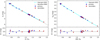 |
Fig. 4 The eclipsing binary components against surface brightness-colour calibrations. The components of the ten eclipsing binaries in this work are shown by blue (primary) or red (secondary) circles. Left: V-band surface brightness versus (V – K) colour relation. Right: Gaia GBP band surface brightness versus (GBP –K) colour relation. |
6.2 Comparison of geometric and eclipsing-binary distances
One of the main reasons for improving the SBCR calibrations is to utilize the SBCRs in precise distance measurements using the eclipsing binary (EB) method. The method relies on Eq. (6): knowing the absolute radii R1,2 of the components and their angular diameters θ1,2 resulting from the SBCR, one can easily derive a distance. The precision of the method is well established, however, its accuracy and the presence of possible systematic effects is not yet fully discussed.
The EB method was used before to verify the zero-point shift of the Gaia parallaxes both in the ‘classical’ way, by means of bolometric flux scaling (Stassun & Torres 2016, 2021), and with the use of SBCRs (Graczyk et al. 2019). Both approaches show near perfect agreement between distances derived from Gaia parallaxes and those inferred from the EB method. However, the accuracy of the ’classical’ approach is limited by the bias on the effective temperature determination, because whatever method is employed it introduces its own unspecified systematic uncertainty on the derived temperatures. On the other hand, the SBCR approach is limited mostly by the systematic uncertainty of calibrations of SBCRs – in that case an approximate measure of the systematic is the rms of the calibration itself.
Nearby EBs within 200 pc are the best for testing the SBCR approach because of typically low interstellar extiction. However, the geometric distances of EBs inferred from Gaia are not only affected by the zero-point uncertainty but also by the photocenter movements and by unresolved tertiary companions (Stassun & Torres 2021). The EB photocenter movements correlate very well with the RUWE parameter and obviously on average the closer is the EB the larger the photocenter movement. Because the Gaia DR3 data reduction does not take the photocenter movements into account, the parallaxes of nearby EBs a contain small and hard-to-specify amount of systematics.
Another way to test the EB method is to compare the SBCR distances against distances based on the orbital (or dynamical) parallaxes provided by astrometric, eclipsing binary stars resolved by optical/near-infrared interferometry. From a number of such systems observed during the last decade we selected 10 EBs which had secure near-infrared magnitudes and determined their precise physical parameters. Our team analyzed five such systems by determining visual semimajor orbital axes using VLT/PIONIER for TZ For (Gallenne et al. 2016, 2018), AI Phe, AL Dor, KW Hya, NN Del (Gallenne et al. 2019) and for two more EBs using VLT/GRAVITY: V963 Cen and LL Aqr (Gallenne et al. 2023). We augmented the sample with three systems from the literature: V923 Sco observed by using VLTI (Pribulla et al. 2018), V1022 Cas and V1143 Cyg observed by using CHARA Array (Lester et al. 2019a,b). The precision of orbital parallaxes of these ten systems is well below 1%.
Additional physical data for all ten systems are taken from Albrecht et al. (2007), Andersen & Vaz (1984), Andersen et al. (1987, 1991), Graczyk et al. (2016, 2021, 2022), Maxted et al. (2020), Southworth (2021), and Sybilski et al. (2018). The V -band magnitudes were collected from SIMBAD database and infrared K-band magnitudes were taken from the 2MASS catalog.
Almost all components of selected EBs are main sequence stars or sub-giants with the exception of the cooler component in TZ For. We employed the SBCR calibrated on the (V–K) colour for main sequence dwarfs. We used the calibration derived from interferometric angular diameters (Kervella et al. 2004) and from eclipsing binary stars (Graczyk et al. 2021). Figure 5 shows a comparison of distances from the SBCR calibrations with distances calculated from precise orbital parallaxes. The agreement between both distances is remarkably good, the residuals are consistent with measurement errors, judging from the reduced  , and no significant systematic deviations can be noticed. We carried out comparisons utilising also (V–J) and (B–K) colours and in both cases we obtained similar results to those based on the (V–K) colour.
New precise SBCR calibrations based on eclipsing binary stars are envisioned in a following paper. We plan to extend a sample of EBs that will be useful for the calibration, both by using the literature data and an analysis of a final sample of EBs based on data from our spectroscopic follow-up with HARPS.
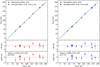 |
Fig. 5 Comparison of distances derived from astrometry and the SBCR for 10 eclipsing binary stars. The SBCR used are Left: Graczyk et al. (2021) and Right: Kervella et al. (2004) and they result is a very good agreement of both distances in terms of the mean and the rms of residuals. For the giant-hosting TZ For (a green circle) the relation by Pietrzyński et al. (2019) was used. |
Data availability
The full Table C.3 is available at the CDS via anonymous ftp to cdsarc.cds.unistra.fr (130.79.128.5) or via https://cdsarc.cds.unistra.fr/viz-bin/cat/J/A+A/694/A65
Acknowledgements
The research leading to these results has received funding from the European Research Council (ERC) Synergy “UniverScale” grant financed by the European Union’s Horizon 2020 research and innovation programme under the grant agreement number 951549, from the National Science Center, Poland grants MAESTRO UMO-2017/26/A/ST9/00446 and BEETHOVEN UMO-2018/31/G/ST9/03050. We acknowledge support from the IdP II 2015 0002 64 and DIR/WK/2018/09 grants of the Polish Ministry of Science and Higher Education. The research was based on data collected under the ESO/CAMK PAN – OCM agreement at the ESO Paranal Observatory. R.S. is supported from the National Science Center, Poland, grant SONATA BIS 2018/30/E/ST9/00598. This work has made use of data from the European Space Agency (ESA) mission Gaia (https://www.cosmos.esa.int/gaia), processed by the Gaia Data Processing and Analysis Consortium (DPAC, https://www.cosmos.esa.int/web/gaia/dpac/consortium). Funding for the DPAC has been provided by national institutions, in particular the institutions participating in the Gaia Multilateral Agreement. This paper includes data collected with the TESS and the Kepler missions, obtained from the MAST data archive at the Space Telescope Science Institute (STScI). Funding for the TESS and the Kepler missions is provided by the NASA Explorer Program. STScI is operated by the Association of Universities for Research in Astronomy, Inc., under NASA contract NAS 5–26555. GP and PK acknowledge the support from the Polish-French Marie Skłodowska-Curie and Pierre Curie Science Prize awarded by the Foundation for Polish Science. NN acknowledges the support of the French Agence Nationale de la Recherche (ANR), under grant ANR-23- CE31-0009-01 (Unlock-pfactor). AG acknowledges the support of the Agencia Nacional de Investigación Científica y Desarrollo (ANID) through the FONDE- CYT Regular grant 1241073. This research has made use of the VizieR catalogue access tool, CDS, Strasbourg, France (DOI : 10.26093/cds/vizier). The original description of the VizieR service was published in Ochsenbein et al. (2000). Based on observations made with ESO Telescopes at the La Silla Paranal Observatory under programmes 0100.D-0339, 0101.D-0697, 0102.D-0281, 105.20L8, 106.20Z1 (PI G. Pietrzyn´ski), 105.2045, 108.21XB (PI D. Graczyk), 099.D- 0380 and 0100.D-0273 (PI W. Gieren). In the analysis we used the uncertainties, lighkurve, astropy, astroquery, tesscut python packages.
Appendix A Comparison with previous studies
A.1 TYC 6511-1799-1
The ASAS data of TYC 6511-1799-1 was used by Shivvers et al. (2014) to derive the orbital period and eccentricity. The eccentricity they calculated is 0.32±0.07 which is much less than our value, probably because the groundbased ASAS photometry is sparse and obviously inferior to TESS.
A deeper analysis was presented by Ratajczak et al. (2021). They used TESS short-cadence data from Sector 6 and radial velocities from spectra obtained with the ESO FEROS and the CTIO CHIRON spectrographs, so basically very similar data as ours. A comparison of the orbital and the physical parameters (their Table 4 and 5) shows very good agreement with our results. However, it must be noted that the parameters we derived, especially masses and radii, are almost an order of magnitude more precise. It should be mentioned is that Ratajczak et al. (2021) defined the secondary minimum as the primary one, so the names of components are reversed.
A.2 TYC 266-718-1 = EPIC 201648133
The K2 light curve from Campaign 01 was analysed by Maxted & Hutcheon (2018) who derived a set of photometric and radiative parameters. The fractional radii r1,2 and the geometry of the orbit (e, ω, i) are consistent to within 2σ with our values, which is reassuring, as we based our final solution on the TESS light curve. The parameters which we derived from K2 data alone are fully consistent (to within 1σ) with those reported by Maxted & Hutcheon (2018), for example the third light and the flux ratio. The temperatures from their SED analysis are also consistent with our adopted temperatures (Table 4) to within 1σ.
More recently Hoyman & Çakırlı (2020) also analysed the K2 data, but supported by HARPS spectra from the ESO archive. They derived radial velocities and presented a full model of the system. However, the analysis and the solution they presented had a number of peculiarities. 1) Model radial velocity curves presented in their Fig. 2 correspond to a much higher orbital eccentricity, of about e ≈ 0.4, than what is observed in the system, i.e. e ≈ 0.05. For such a small e the radial velocity curve looks a sinusoid, regardless what the value of ω is – compare with our Fig. B.3. Strangely, they reported in their Table 2 the low and correct value of e = 0.052(17), which is inconsistent with their Fig. 2. 2) The radial velocities they derived and presented in Table A.1 are inexplicably very different from the values we derive. The shifts amount to 20-40 km s–1, depending on the spectroscopic epoch and on the component. Subsequently, they derive model parameters which are inconsistent with ours, most notably the mass ratio. 3) The high T2/T1 temperature ratio they derive from ISPEC analysis is obviously in large tension with both K2 and TESS light curves (i.e. primary and secondary eclipse have similar depth), but also with our results from the atmospheric analysis of the decomposed HARPS spectra. 4) Errors on parameters reported by Hoyman & Çakırlı (2020) are suspiciously large taking into acccount the superb quality of the K2 and the HARPS data. In summary: it was impossible to make any reasonable comparison with the results obtained by Hoyman & Çakırlı (2020).
A.3 HD 149946 = EPIC 202674012
The system is well investigated thanks to K2 data and the spectroscopic follow-up by Hełminiak et al. (2018). A comparison with the previously published reports is presented in Table A.1. The model parameters reported by Maxted & Hutcheon (2018) and Hełminiak et al. (2021) are fully consistent with those from our best model. Especially the agreement with results obtained by Hełminiak et al. (2021) is striking, taking into account the small uncertainties reported. The only significant difference is between the orbital inclination, which is most probably a result of the inclusion of the TESS light curve in our analysis. Also we obtain slightly larger errors on stellar radii to accommodate the difference in the fractional radii obtained when K2 and TESS data are solved separately. Again, the analysis presented by Hoyman & Çakırlı (2020) has some oddities like in a case of TYC 266-718-1. For example in their Table A.1, they present radial velocity determinations from HARPS spectra, but only for the primary component. Strangely, the RVs for the secondary are not listed despite the fact that absorption lines of the secondary are easy to identify in the HARPS spectra. In general, the agreement of their results with ours is poor.
A.4 HD 219869 = EPIC 246024234
The system was previously analysed by Hełminiak et al. (2021) who used the K2 photometry supplemented with 12 FEROS and three HARPS spectra. Like in the case of HD 149946, we find very good consistency with their results. Most parameters from their Table 3 are within 1σ agreement with our parameters listed in Tables C.4 and 5. However, there are some larger differences: the orbital inclination i differs by 2σ, most probably because we included TESS data in the analysis. The largest difference of 4σ appears in the primary’s effective temperature: Hełminiak et al. (2021) report a low temperature similar to the secondary’s temperature, however the relative depth of eclipses in both the K2 and TESS light curves, as well as our atmospheric analysis of decomposed spectra indicate clearly that the primary is significantly hotter than the secondary.
Comparison of our results for HD 149946 with literature values.
Appendix B Figures
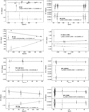 |
Fig. B.1 O-C diagrams for all eccentric systems in our sample. Primary minima are marked with darker circles. |
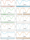 |
Fig. B.2 Best WD model fits to the photometry of the ten eclipsing binary stars in our sample and their residuals. Coloured points: observations, black line: synthetic light curve. |
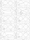 |
Fig. B.3 Best WD model fits to the HARPS velocimetry of the ten eclipsing binary stars in our sample and their residuals. Filled circles: primary component, open circles: secondary component. Black lines: model predictions. |
Appendix C Tables
Photometric observations used for the light curve analysis in the present study.
Spectroscopic observations with HARPS.
RV measurements for eclipsing binary stars. The full data are available at the CDS.
Model parameters from the Wilson-Devinney code
References
- Albrecht, S., Reffert, S., Snellen, I., Quirrenbach, A., & Mitchell, D. S. 2007, A&A, 474, 565 [NASA ADS] [CrossRef] [EDP Sciences] [Google Scholar]
- Allard, F., Homeier, D., Freytag, B., et al. 2013, Mem. Soc. Astron. Ital. Suppl., 24, 128 [Google Scholar]
- Alonso, A., Arribas, S., & Martínez-Roger, C. 1996, A&A, 313, 873 [Google Scholar]
- Andersen, J., & Vaz, L. P. R. 1984, A&A, 130, 102 [NASA ADS] [Google Scholar]
- Andersen, J., García, J. M., Giménez, A., et al. 1987, A&A, 174, 107 [NASA ADS] [Google Scholar]
- Andersen, J., Clausen, J. V., Nordstrom, B., Tomkin, J., & Mayor, M. 1991, A&A, 246, 99 [NASA ADS] [Google Scholar]
- Armstrong, D. J., Kirk, J., Lam, K. W. F., et al. 2015, A&A, 579, A19 [NASA ADS] [CrossRef] [EDP Sciences] [Google Scholar]
- Barros, S. C. C., Demangeon, O., & Deleuil, M. 2016, A&A, 594, A100 [NASA ADS] [CrossRef] [EDP Sciences] [Google Scholar]
- Bessell, M. S., & Brett, J. M. 1988, PASP, 100, 1134 [Google Scholar]
- Boyajian, T. S., van Belle, G., & von Braun, K. 2014, AJ, 147, 47 [Google Scholar]
- Breuval, L., Riess, A. G., Casertano, S., et al. 2024, ApJ, submitted [arXiv:2404.08038] [Google Scholar]
- Caldwell, D. A., Tenenbaum, P., Twicken, J. D., et al. 2020, RNAAS, 4, 201 [NASA ADS] [Google Scholar]
- Capitanio, L., Lallement, R., Vergely, J. L., Elyajouri, M., & Monreal-Ibero, A. 2017, A&A, 606, A65 [NASA ADS] [CrossRef] [EDP Sciences] [Google Scholar]
- Carpenter J. M., 2001, AJ, 121, 2851 [NASA ADS] [CrossRef] [Google Scholar]
- Casagrande, L., Ramírez, I., Meléndez, J., Bessell, M., & Asplund, M. 2010, A&A, 512, A54 [NASA ADS] [CrossRef] [EDP Sciences] [Google Scholar]
- Coelho, P., Barbuy, B., Meléndez, J., Schiavon, R. P., & Castilho, B. V. 2005, A&A, 443, 735 [NASA ADS] [CrossRef] [EDP Sciences] [Google Scholar]
- Cutri, R. M., Skrutskie, M. F., van Dyk, S., et al. 2003, VizieR Online Data Catalogue: II/246 [Google Scholar]
- Cutri, R. M., Wright, E. L., Conrow, T., et al. 2012, VizieR Online Data Catalog: II/311 [Google Scholar]
- Díaz, C. G., González, J. F., Levato, H., & Grosso, M. 2011, A&A, 531, A143 [NASA ADS] [CrossRef] [EDP Sciences] [Google Scholar]
- Flower, P. J. 1996, ApJ, 469, 355 [NASA ADS] [CrossRef] [Google Scholar]
- Foreman-Mackey, D., Hogg, D. W., Lang, D., et al. 2013, PASP, 125, 306 [NASA ADS] [CrossRef] [Google Scholar]
- Fouqué, P., & Gieren, W. P. 1997, A&A, 320, 799 [Google Scholar]
- Gaia Collaboration (Prusti, T., et al.) 2016, A&A, 595, A1 [NASA ADS] [CrossRef] [EDP Sciences] [Google Scholar]
- Gaia Collaboration (Brown, A. G. A., et al.) 2021, A&A, 649, A1 [NASA ADS] [CrossRef] [EDP Sciences] [Google Scholar]
- Gaia Collaboration (Vallenari, A., et al.) 2023, A&A, 674, A1 [NASA ADS] [CrossRef] [EDP Sciences] [Google Scholar]
- Gallenne, A., Pietrzynski, G., Graczyk, D., et al. 2016, A&A, 586, A35 [NASA ADS] [CrossRef] [EDP Sciences] [Google Scholar]
- Gallenne, A., Pietrzynski, G., Graczyk, D., et al. 2018, A&A, 616, A68 [NASA ADS] [CrossRef] [EDP Sciences] [Google Scholar]
- Gallenne, A., Pietrzynski, G., Graczyk, D., et al. 2019, A&A, 632, A31 [NASA ADS] [CrossRef] [EDP Sciences] [Google Scholar]
- Gallenne, A., Mérand, A., Kervella, P., et al. 2023, A&A, 672, A119 [NASA ADS] [CrossRef] [EDP Sciences] [Google Scholar]
- Giménez, A., & Bastero, M. 1995, Ap&SS, 226, 99 [Google Scholar]
- González, J. F., & Levato, H. 2006, A&A, 448, 283 [NASA ADS] [CrossRef] [EDP Sciences] [Google Scholar]
- González Hernández, J. I., & Bonifacio, P. 2009, A&A, 497, 497 [Google Scholar]
- Graczyk, D., Pietrzynski, G., Thompson, I. B., et al. 2014, ApJ, 780, 59 [Google Scholar]
- Graczyk, D., Smolec, R., Pavlovski, K., et al. 2016, A&A, 594, A92 [NASA ADS] [CrossRef] [EDP Sciences] [Google Scholar]
- Graczyk, D., Konorski, P., Pietrzynski, G., et al. 2017, ApJ, 837, 7 [NASA ADS] [CrossRef] [Google Scholar]
- Graczyk, D., Pietrzynski, G., Gieren, W., et al. 2019, ApJ, 872, 85 [NASA ADS] [CrossRef] [Google Scholar]
- Graczyk, D., Pietrzynski, G., Thompson, I. B., et al. 2020, ApJ, 904, 13 [Google Scholar]
- Graczyk, D., Pietrzynski, G., Galan, C., et al. 2021, A&A, 649, A109 [NASA ADS] [CrossRef] [EDP Sciences] [Google Scholar]
- Graczyk, D., Pietrzynski, G., Galan, C., et al. 2022, A&A, 666, A128 [NASA ADS] [CrossRef] [EDP Sciences] [Google Scholar]
- Gray, D. F. 2005, The Observation and analysis of Stellar Photospheres (New York: Cambridge University Press) [Google Scholar]
- Gray, D. F., Graham, P. W., & Hoyt, S. R., 2001, AJ, 121, 2159 [Google Scholar]
- Groenewegen, M. A. T. 2004, MNRAS, 353, 903 [Google Scholar]
- Guo, Z., Gies, D. R., & Fuller, J. 2017, ApJ, 834, 59 [Google Scholar]
- Gustafsson, B., Edvardsson, B., Eriksson, K., et al. 2008, A&A, 486, 951 [NASA ADS] [CrossRef] [EDP Sciences] [Google Scholar]
- Güzel, O., & Özdarcan, O. 2020, Contrib. Astron. Observ. Skalnate Pleso, 50, 535 [Google Scholar]
- Hardegree-Ullman, K. K., Zink, J. K., Christiansen, J. L., et al. 2020, ApJS, 247, 28 [NASA ADS] [CrossRef] [Google Scholar]
- Helminiak, K. G., Jordán, A., Espinoza, N., et al. 2018, RNAAS, 2, 226 [NASA ADS] [Google Scholar]
- Helminiak, K. G., Moharana, A., Pawar, T., et al. 2021, MNRAS, 508, 5687 [CrossRef] [Google Scholar]
- Hindsley, R. B., & Bell, R. A. 1989, ApJ, 341, 1004 [Google Scholar]
- Hoffleit, D., & Jaschek, C. 1991, The Bright Star Catalog, 5th rev. (New Haven, Conn.: Yale University Observatory) [Google Scholar]
- Houdashelt, M. L., Bell, R. A., & Sweigert, A. V. 2000, AJ, 119, 1448 [Google Scholar]
- Houk, N. 1978, University of Michigan Catalogue of Two Dimensional Spectral Types for the HD stars, 2. Declinations –52 to –40, eds. N. Houk (Ann Arbor: Department of Astronomy, University of Michigan: distributed by University Microfilms International) [Google Scholar]
- Houk, N. 1982, Michigan Catalogue of Two-dimensional Spectral Types for the HD stars, 3. Declinations –40_0 to –26_0., ed. N. Houk (Ann Arbor, MI (USA): Department of Astronomy, University of Michigan), 12 + 390 [Google Scholar]
- Houk, N., & Swift, C. 1999, Michigan Catalogue of Two-dimensional Spectral Types for the HD Stars, 5, eds. N. Houk & C. Swift (Ann Arbor, Michigan: Department of Astronomy, University of Michigan) [Google Scholar]
- Howell, S. B., Sobeck, C., Haas, M., et al. 2014, PASP, 126, 398 [Google Scholar]
- Hoyman, B., & Çakirli, Ö. 2020, MNRAS, 493, 2329 [CrossRef] [Google Scholar]
- Huang, C. X., Vanderburg, A., Pál, A., et al. 2020, RNAAS, 4, 204 [Google Scholar]
- Jarrett, T. H., Cohen, M., Masci, F., et al. 2011, ApJ, 735, 112 [Google Scholar]
- Jenkins, J. M., Twicken, J. D., McCauliff, S., et al. 2016, Proc. SPIE, 9913, 99133E [Google Scholar]
- Justesen, A. B., & Albrecht, S. 2021, ApJ, 912, 123 [NASA ADS] [CrossRef] [Google Scholar]
- Kazarovets, E. V., Samus, N. N., Durlevich, O. V., et al. 1999, Inform. Bull. Variable Stars, 4659, 1 [Google Scholar]
- Kazarovets, E. V., Samus, N. N., Durlevich, O. V., et al. 2006, Inform. Bull. Variable Stars, 5721, 1 [Google Scholar]
- Kazarovets, E. V., Samus, N. N., Durlevich, O. V., et al. 2008, Inform. Bull. Variable Stars, 5863, 1 [Google Scholar]
- Kervella, P., Thévenin, F., Di Folco, E., & Ségransan, D., 2004, A&A, 426, 297 [NASA ADS] [CrossRef] [EDP Sciences] [Google Scholar]
- Kervella, P., Arenou, F., & Thévenin, F. 2022, A&A, 657, A7 [NASA ADS] [CrossRef] [EDP Sciences] [Google Scholar]
- Kim, C.-H., Kreiner, J. M., Zakrzewski, B., et al. 2018, ApJS, 235, 41 [Google Scholar]
- Klinglesmith, D. A., & Sobieski, S. 1970, AJ, 75, 175 [Google Scholar]
- Koch, D. G., Borucki, W. J., Basri, G., et al. 2010, ApJ, 713, L79 [Google Scholar]
- Kreiner, J. M. 2004, Acta Astron., 54, 207 [NASA ADS] [Google Scholar]
- Kruszewski, A., & Semeniuk, I. 1999, Acta Astron., 49, 561 [NASA ADS] [Google Scholar]
- Lacy, C. H. 1977b, ApJ, 213, 458 [Google Scholar]
- Landstreet, J. D., Kupka, F., Ford, H. A., et al. 2009, A&A, 503, 973 [NASA ADS] [CrossRef] [EDP Sciences] [Google Scholar]
- Lester, K. V., Gies, D. R., Schaefer, G. H., et al. 2019a, AJ, 157, 140 [Google Scholar]
- Lester, K. V., Gies, D. R., Schaefer, G. H., et al. 2019b, AJ, 158, 218 [NASA ADS] [CrossRef] [Google Scholar]
- Lightkurve Collaboration (Cardoso, J. V. et al.) 2018, Astrophysics Source Code Library [record ascl:1812.013] [Google Scholar]
- Ligi, R., Mourard, D., Bério, P., et al. 2023, SF2A-2023: Proceedings of the Annual meeting of the French Society of Astronomy and Astrophysics, 421 [Google Scholar]
- Lindegren, L., Klioner, S., Hernández, J., et al. 2020, A&A, 649, A2 [Google Scholar]
- Lindegren, L., Bastian. U., Biermann, B., et al. 2021, A&A, 649, A4 [NASA ADS] [CrossRef] [EDP Sciences] [Google Scholar]
- Luger, R., Agol, E., Kruse, E., et al. 2016, AJ, 152, 100 [Google Scholar]
- Martin, D. C., Fanson, J., Schiminovich, D., et al. 2005, ApJ, 619, L1 [Google Scholar]
- Masana, E., Jordi, C., & Ribas, I. 2006, A&A, 450, 735 [NASA ADS] [CrossRef] [EDP Sciences] [Google Scholar]
- Maxted, P. F. L., & Hutcheon, R. J. 2018, A&A, 616, A38 [NASA ADS] [CrossRef] [EDP Sciences] [Google Scholar]
- Maxted, P. F. L., Gaulme, P., Graczyk, D., et al. 2020, MNRAS, 498, 332 [Google Scholar]
- Mayor M., Pepe, F., Queloz, D., et al., 2003, The Messenger, 114, 20 [NASA ADS] [Google Scholar]
- Metanomski, A. D. F., Pasquini, L., Krautter, J., et al. 1998, A&AS, 131, 197 [NASA ADS] [CrossRef] [EDP Sciences] [Google Scholar]
- Miller, N. J., Maxted, P. F. L., & Smalley, B. 2020, MNRAS, 497, 2899 [Google Scholar]
- Mould, J. 2019, PASP, 131, 094201 [NASA ADS] [CrossRef] [Google Scholar]
- Mourard, D., Berio, P., Pannetier, C., et al. 2022, Proc. SPIE, 12183, 1218308 [NASA ADS] [Google Scholar]
- Munari, U., & Zwitter, T. 1997, A&A, 318, 269 [NASA ADS] [Google Scholar]
- Onken, C. A., Wolf, C., Bessell, M. S., et al. 2024, arXiv e-prints [arXiv:2402.02015] [Google Scholar]
- Ochsenbein, F.,Bauer, P., & Marcout, J. 2000, Astron. Astrophys. Suppl. Ser., 143, 23 [NASA ADS] [CrossRef] [EDP Sciences] [Google Scholar]
- Otero, S. A., & Wils, P. 2005, Inform. Bull. Variable Stars, 5644, 1 [Google Scholar]
- Perryman, M. A. C., Lindegren, L., Kovalevsky, J., et al. 1997, A&A, 500, 501 [NASA ADS] [Google Scholar]
- Pietrzyński, G., Graczyk, D., Gieren, W., et al. 2013, Nature, 495, 76 [Google Scholar]
- Pietrzyński, G., Graczyk, D., Gallenne, A., et al. 2019, Nature, 567, 200 [Google Scholar]
- Pilecki, B., Gieren, W., Smolec, R., et al. 2017, ApJ, 842, 110 [Google Scholar]
- Pojmanski, G. 2002, Acta Astron., 52, 397 [NASA ADS] [Google Scholar]
- Pojmanski, G. 2003, Acta Astron., 53, 341 [NASA ADS] [Google Scholar]
- Pollacco, D. L., Skillen, I., Collier Cameron, A., et al. 2006, PASP, 118, 1407 [NASA ADS] [CrossRef] [Google Scholar]
- Poznanski, D., Prochaska, J. X., & Bloom, J. S. 2012, MNRAS, 426, 1465 [Google Scholar]
- Pribulla, T., Mérand, A., Kervella, P., et al. 2018, A&A, 616, A49 [NASA ADS] [CrossRef] [EDP Sciences] [Google Scholar]
- Prša, A., Harmanec, P., Torres, G., et al. 2016, AJ, 152, 41 [Google Scholar]
- Prša, A., Kochoska, A., Conroy, K. E., et al. 2022, ApJS, 258, 16 [CrossRef] [Google Scholar]
- Qian, S.-B., Zhang, J., He, J.-J., et al. 2018, ApJS, 235, 5 [NASA ADS] [CrossRef] [Google Scholar]
- Ramírez, I., & Meléndez, J. 2005, ApJ, 626, 465 [Google Scholar]
- Ratajczak, M., Pawlaszek, R. K., Helminiak, K. G., et al. 2021, MNRAS, 500, 4972 [Google Scholar]
- Ricker, G. R., Winn, J. N., Vanderspek, R., et al. 2015, J. Astron. Telesc. Instrum. Syst., 1, 014003 [Google Scholar]
- Riess, A. G., Casertano, S., Yuan, W., et al. 2019, ApJ, 876, 85 [Google Scholar]
- Riess, A. G., Yuan, W., Macri, L. M., et al. 2022, ApJ, 934, L7 [NASA ADS] [CrossRef] [Google Scholar]
- Rucinski, S. M. 1992, AJ, 104, 1968 [Google Scholar]
- Rucinski, S. M. 1999, in Precise Stellar Radial Velocities, ASP Conference Series 185, IAU Colloquium 170, eds. J. B. Hearnshaw, & C. D. Scarfe, 82 [Google Scholar]
- Salsi, A., Nardetto, N., Mourard, D., et al. 2020, A&A, 640, A2 [NASA ADS] [CrossRef] [EDP Sciences] [Google Scholar]
- Salsi, A., Nardetto, N., Mourard, D., et al. 2021, A&A, 652, A26 [NASA ADS] [CrossRef] [EDP Sciences] [Google Scholar]
- Salsi, A., Nardetto, N., Plez, B., & Mourard, D. 2022, A&A, 662, A120 [NASA ADS] [CrossRef] [EDP Sciences] [Google Scholar]
- Sheminova, V. A., 2019, KPCB, 35, 129 [NASA ADS] [Google Scholar]
- Shivvers, I., Bloom, J. S., & Richards, J. W. 2014, MNRAS, 441, 343 [NASA ADS] [CrossRef] [Google Scholar]
- Shulyak, D., Tsymbal, V., Ryabchikova, T. A., et al., 2004, A&A, 428, 993 [NASA ADS] [CrossRef] [EDP Sciences] [Google Scholar]
- Skrutskie, M. F., Cutri, R. M., Stiening, R., et al. 2006, AJ, 131, 1163 [NASA ADS] [CrossRef] [Google Scholar]
- Smalley, B., 2014, in Determination of Atmospheric Parameters of B-, A-, F-, and G-type stars, Lectures fom the School of Spectroscopic Data Analyses eds. E. Niemczura, B. Smalley, & W. Pych (Springer), 131 [Google Scholar]
- Southworth, J. 2021, The Observatory, 141, 52 [NASA ADS] [Google Scholar]
- Stassun, K. G., & Torres, G. 2016, AJ, 152, 180 [Google Scholar]
- Stassun, K. G., & Torres, G. 2021, ApJ, 907, L33 [NASA ADS] [CrossRef] [Google Scholar]
- Sybilski, P., Pawlaszek, R. K., Sybilska, A., et al. 2018, MNRAS, 478, 1942 [NASA ADS] [CrossRef] [Google Scholar]
- Thompson, I. B., Kaluzny, J., Pych, W., et al. 2001, AJ, 121, 3089 [NASA ADS] [CrossRef] [Google Scholar]
- Tkachenko, A., 2015, A&A, 581, A129 [NASA ADS] [CrossRef] [EDP Sciences] [Google Scholar]
- Tsymbal, V., 1996, ASPC, 108, 198 [Google Scholar]
- van Hamme W., 1993, AJ, 106, 2096 [CrossRef] [Google Scholar]
- van Hamme, W., & Wilson, R. E. 2007, ApJ, 661, 1129 [Google Scholar]
- Williams, S. J., Gies, D. R., Helsel, J. W., et al. 2011, AJ, 142, 5 [NASA ADS] [CrossRef] [Google Scholar]
- Wilson, R. E. 1979, ApJ, 234, 1054 [Google Scholar]
- Wilson, R. E. 1990, ApJ, 356, 613 [Google Scholar]
- Wilson, R. E., & Devinney, E. J. 1971, ApJ, 166, 605 [Google Scholar]
- Wilson, R. E., & Van Hamme, W. 2014, ApJ, 780, 151 [Google Scholar]
- Worthey, G., & Lee, H., 2011, ApJS, 193, 1 [Google Scholar]
- Wraight, K. T., White, G. J., Bewsher, D., et al. 2011, MNRAS, 416, 2477 [NASA ADS] [CrossRef] [Google Scholar]
All Tables
Photometric observations used for the light curve analysis in the present study.
RV measurements for eclipsing binary stars. The full data are available at the CDS.
All Figures
|
Fig. 1 5054 – 5257 Å (top) and 5608–5884 Å (bottom) regions of disentangled spectra of the primary and the secondary components of AW Col with selected spectral lines identified. Strong lines from ionised yttrium (Y II λ 5087.42, 5200.41, 5205.72, and 5662.92 Å), and barium (Ba II λ 5853.67 Å) are visible. The red lines denote the atmosphere model fits to the observed spectra (blue). The gray shaded areas were excluded from calculations by the use of an individual mask. |
| In the text | |
|
Fig. 2 Relation between the equivalent width of the sodium line D1 and the reddening. |
| In the text | |
|
Fig. 3 Out-of-eclipse variations of VZ PsA between two consecutive secondary minima. Different parts of TESS Sectors 01 and 28 are shifted vertically for a better view. The larger brightening occurs near the periastron passage (BJD 2459072). |
| In the text | |
|
Fig. 4 The eclipsing binary components against surface brightness-colour calibrations. The components of the ten eclipsing binaries in this work are shown by blue (primary) or red (secondary) circles. Left: V-band surface brightness versus (V – K) colour relation. Right: Gaia GBP band surface brightness versus (GBP –K) colour relation. |
| In the text | |
|
Fig. 5 Comparison of distances derived from astrometry and the SBCR for 10 eclipsing binary stars. The SBCR used are Left: Graczyk et al. (2021) and Right: Kervella et al. (2004) and they result is a very good agreement of both distances in terms of the mean and the rms of residuals. For the giant-hosting TZ For (a green circle) the relation by Pietrzyński et al. (2019) was used. |
| In the text | |
|
Fig. B.1 O-C diagrams for all eccentric systems in our sample. Primary minima are marked with darker circles. |
| In the text | |
|
Fig. B.2 Best WD model fits to the photometry of the ten eclipsing binary stars in our sample and their residuals. Coloured points: observations, black line: synthetic light curve. |
| In the text | |
|
Fig. B.3 Best WD model fits to the HARPS velocimetry of the ten eclipsing binary stars in our sample and their residuals. Filled circles: primary component, open circles: secondary component. Black lines: model predictions. |
| In the text | |
Current usage metrics show cumulative count of Article Views (full-text article views including HTML views, PDF and ePub downloads, according to the available data) and Abstracts Views on Vision4Press platform.
Data correspond to usage on the plateform after 2015. The current usage metrics is available 48-96 hours after online publication and is updated daily on week days.
Initial download of the metrics may take a while.