| Issue |
A&A
Volume 691, November 2024
|
|
|---|---|---|
| Article Number | A54 | |
| Number of page(s) | 13 | |
| Section | The Sun and the Heliosphere | |
| DOI | https://doi.org/10.1051/0004-6361/202450046 | |
| Published online | 29 October 2024 | |
Statistical study of the peak and fluence spectra of solar energetic particles observed over four solar cycles
1
Deep Space Exploration Laboratory/School of Earth and Space Sciences, University of Science and Technology of China, Hefei 230026, China
2
CAS Center for Excellence in Comparative Planetology, University of Science and Technology of China, Hefei 230026, China
3
Collaborative Innovation Center of Astronautical Science and Technology, Harbin 150001, China
⋆ Corresponding author; This email address is being protected from spambots. You need JavaScript enabled to view it.
Received:
20
March
2024
Accepted:
3
August
2024
Abstract
Context. Solar energetic particles (SEPs) are an important space radiation source, especially for the space weather environment in the inner heliosphere. The energy spectrum of SEP events is crucial both for evaluating their radiation effects and for understanding their acceleration process at the source region, along with their propagation mechanism.
Aims. In this work, we investigate the properties of the SEP peak flux spectra and the fluence spectra and their potential formation mechanisms using statistical methods. We aim to advance our understanding of SEP acceleration and propagation mechanisms.
Methods. Employing a dataset from the European Space Agency’s Solar Energetic Particle Environment Modelling (SEPEM) program, we obtained and fit the peak-flux and fluence proton spectra of more than a hundred SEP events from 1974 to 2018. We analyzed the relationship among the solar activity, X-ray peak intensity of solar flares, and the SEP’s spectral parameters.
Results. Based on the assumption that the initial spectrum of accelerated SEPs generally displays a power-law distribution and that the diffusion coefficient has a power-law dependence on the particle energy, we can assess both the source and propagation properties using the observed SEP event peak flux and fluence energy spectra. We confirm that the spectral properties of SEPs are influenced by the solar source and the interplanetary conditions, whereas their transportation process can be influenced by different phases of solar cycle.
Conclusions. This study provides an observational perspective on the double power-law spectral characteristics of the SEP energy spectra, revealing their correlation with the adiabatic cooling and diffusion processes during the particle propagation from the Sun to the observer. This result contributes to forging a deeper understanding of the acceleration and propagation of SEP events, in particular, the possible origins of the double power law.
Key words: Sun: activity / Sun: evolution / Sun: flares / Sun: heliosphere / Sun: particle emission / solar-terrestrial relations
© The Authors 2024
 Open Access article, published by EDP Sciences, under the terms of the Creative Commons Attribution License (https://creativecommons.org/licenses/by/4.0), which permits unrestricted use, distribution, and reproduction in any medium, provided the original work is properly cited.
This article is published in open access under the Subscribe to Open model. This email address is being protected from spambots. You need JavaScript enabled to view it. to support open access publication.
1. Introduction
To carry out space exploration activities, we need to have a clear understanding of the radiation environment in space. The energy spectrum of high-energy particles in space is a direct input for evaluating radiation doses. As the ultimate source, the Sun not only releases high-energy charged particles, but also significantly affects the propagation of particles. Thus, the observed energy spectrum varies due to the different properties of particle acceleration and propagation processes. Various studies have attempted to use the observed data and existing knowledge to reconstruct these two aspects (see, e.g., Klein & Dalla 2017, and references therein).
Typically, there are two mechanisms contributing to the acceleration of charged particles (Reames 1999, 2013): magnetic reconnection acceleration associated with flares and shock wave acceleration associated with coronal mass ejections (CMEs). Ideally, we may be able to distinguish different acceleration processes by comparing the composition and state of particles in the chromosphere and corona, such as proton-to-electron ratios, 3He compositions, and ion charge states (Mason 2007; Klein & Dalla 2017). However, due to the fact that a SEP event is often associated with the onsets of both a solar flare and a CME, it is difficult to distinguish the role of the two types of acceleration processes. Furthermore, tracking the source of SEP events becomes more challenging when considering the propagation process of particles (see, e.g., Guo et al. 2024, and references therein).
Once SEPs are released into interplanetary space, their propagation can be theoretically described by the Fokker-Planck equation (Parker 1965) as follows:
![Mathematical equation: $$ \begin{aligned} \frac{\partial U}{\partial t}&=-\frac{V_{sw}}{r^{2}} \frac{\partial }{\partial r}\left(r^{2} U\right)+\frac{2 V_{sw}}{3 r} \frac{\partial }{\partial E}[UEn(E)]+\frac{1}{r^{2}} \frac{\partial }{\partial r}\left(\kappa r^{2} \frac{\partial U}{\partial r}\right); \end{aligned} $$](/articles/aa/full_html/2024/11/aa50046-24/aa50046-24-eq1.gif) (1)
(1)
 (2)
(2)
Here U(r, E, t) represents the probability distribution over the kinetic energy, E, for the location, r, and time t; Vsw is the solar wind speed; κ is the diffusion coefficient; and m0 is the rest mass of the particle; finally, n(E) represents the normalized conversion coefficient between the particle momentum, p, and kinetic energy, E. For relativistic particles, n(E)≈1, and for non-relativistic particles, n(E)≈2. The terms on the right-hand side of Eq. (1) originate from three particle transport mechanisms: convection, adiabatic cooling, and diffusion. Each of these transport mechanisms may modify the original acceleration characteristics of energetic particles.
In this study, we focus on the properties of SEP proton energy spectra and carry out a statistical investigation of the correlation between solar activity index and the properties of SEP events. We aim to extract information about the acceleration and propagation processes of SEPs combining analytical descriptions of particle propagation and parameters obtained from observations. Analytical details on the SEP energy spectra are introduced in Sect. 2. The dataset, SEP event list, and fitting method are given in Sect. 3. Subsequently, we examine the distributions of SEP proton energy spectra parameters, as well as the relationships between integral fluence spectra and peak flux spectra and how they change with the solar cycle in Sect. 4. Our results and conclusions are summarized in Sect. 5.
2. Analytical descriptions of the SEP energy spectra
The SEP energy spectrum is the flux distribution of SEPs versus the particle energy, which is determined by both the acceleration process and transport effects. The SEP spectrum can be directly measured by high-energy particle detectors in space, and some large SEP events can also be indirectly recorded by ground neutron detectors or muon detectors when the secondary particles have energy high enough to reach the surface of Earth. These are also known as ground-level enhancement (GLE) events (see, e.g., Sect. 3 of Guo et al. 2024, and references therein). By adopting different integration time windows, we can study the event energy spectrum and its time evolution. The most frequently referenced one is the integrated fluence spectrum of the entire event. This spectrum accumulates the flux of particles over different energies from the beginning to the end of the event and is crucial for evaluating the total radiation effect of the event. Another important one is the time-of-maximum (TOM) energy spectrum or peak flux spectrum formed by the maximum flux at each energy bin. This method can minimize the impact of solar wind on energetic particle propagation processes, such as diffusion, convection, and velocity dispersion effects, allowing for a more reasonable estimation of the energy spectrum of the source region (Hollebeke & Ma Sung 1975).
2.1. Integral fluence spectra
Previous studies have proposed multiple functions to describe the integral fluence spectra of SEP events. The most commonly used functions are the single power law with an exponential rollover function (e.g., Tylka 2001) and the double power-law function (e.g., Mewaldt et al. 2012; Raukunen et al. 2018). The latter is also called the “Band” function, which was originally proposed for fitting γ-ray burst spectra (Band et al. 1993). It has been confirmed that the Band formulation generally fits SEP integral fluence spectra better, especially for those large-scale events (e.g., Mewaldt et al. 2005). Therefore, we chose this function to fit SEP integral fluence spectra in this study. Here, the Band function is given as:
![Mathematical equation: $$ \begin{aligned} \frac{d J}{d E}=\left\{ \begin{array}{ll}&C E^{\gamma _{1}} \exp \left(-E / E_{0}\right) ,\\&\text{ if} E <\left(\gamma _{1}-\gamma _{2}\right) E_{0}; \\&C E^{\gamma _{2}}\left\{ \left[\left(\gamma _{1}-\gamma _{2}\right) E_{0}\right]^{\left(\gamma _{1}-\gamma _{2}\right)} \exp \left(\gamma _{2}-\gamma _{1}\right)\right\} , \\&\text{ if} E \ge \left(\gamma _{1}-\gamma _{2}\right) E_{0}. \end{array}\right. \end{aligned} $$](/articles/aa/full_html/2024/11/aa50046-24/aa50046-24-eq3.gif) (3)
(3)
where C is an overall fluence normalization coefficient in the same units of dJ/dE; γ1 is the power-law index at the low-energy range; γ2 is the power-law index at the high-energy range; E is particle’s kinetic energy as defined in Eq. (1); E and E0 are measured in energy/nucleon; and (γ1 − γ2)E0 is break-point energy that separates the low-energy and high-energy ranges. Both the Band function and its first derivative are continuous at this break point. However, we must note that there is no clear physical meaning of the four free parameters of Band function and this function is still a semi-phenomenological model. Due to the mixing of propagation effects, such as diffusion and adiabatic cooling, it is difficult to directly obtain information on the source and propagation process of high-energy particles through the parameters defined by the integrated energy spectra. These aspects are further discussed in Sects. 4 and 5.
2.2. Peak flux spectra
When neglecting convection and adiabatic deceleration terms, the transportation of energetic particles can be treated as a process of simple time-dependent spherical diffusion from a point source. Then the time profile of a well-connected SEP event flux can be described by a simple function (e.g., Parker 1963) as follows:
 (4)
(4)
where j(p, r, t) is particle’s flux at a location, r, time, t, with a momentum, p, and κ(p) is energy-dependent diffusion coefficient, while N0(p) is the number of particles per unit momentum released at the Sun. From Eq. (4), we can derive the peak flux spectrum for t = tmax = r2/(6κ(p)) and see that peak flux spectrum has the same shape with the source spectrum (Forman et al. 1986):
 (5)
(5)
For the early stages of SEP events, the convective effect of particle propagation can be ignored compared to the diffusion effect (e.g., McCracken et al. 1971). When considering adiabatic deceleration and assuming a simple power-law diffusion coefficient as:
 (6)
(6)
Kurt et al. (1981) estimated the particle’s adiabatic energy loss ΔE as:
 (7)
(7)
where Es is the particle’s kinetic energy directly being released at the Sun, then E is the particle’s kinetic energy at a location, r, Vsw is the solar wind speed, κ0 is the normalization coefficient in the same unit of diffusion coefficient, κ, and α is the power-law index.
Previous studies have shown that for the two acceleration processes of SEPs, it is relatively reasonable to assume that the energy spectrum after acceleration follows a simple power-law (e.g., Jones & Ellison 1991; Dierckxsens et al. 2015; Fu et al. 2006):
 (8)
(8)
where j0 is the normalization coefficient in the same units of particle’s flux, j, and γ is the index of the power-law energy spectrum after acceleration. Based on the conservation of particle number and combined with Eq. (7), the particle energy spectrum at location, r, can be obtained as:
 (9)
(9)
Figure 1 illustrates the impact of adiabatic energy loss on the spectrum, as described by the above equation. We set an initial flux spectrum with the parameters j0 = 108[#/cm2/s/sr/MeV], γ = 4, and a constant solar wind speed of Vsw = 450 [km/s]. Panel a shows the peak flux spectra at 1 AU for different diffusion coefficient indexes, α. Panel b shows the adiabatic energy loss of particles with a given initial energy corresponding to Panel a. Panel c shows the peak flux spectra at 1 AU with different diffusion normalization coefficients, κ0. Panel d shows the adiabatic energy loss of particles with a given initial energy corresponding to Panel c. Panel e shows the evolution of the peak flux spectrum at different heliocentric distances. Panel f shows the adiabatic energy loss corresponding to Panel e. From this graph, it can be seen that smaller diffusion coefficients, namely smaller κ0 and α values, will have a more pronounced adiabatic cooling effect on particles, especially for those with lower energy (less than tens of MeV). Additionally, as the propagation distance increases, the peak energy spectrum of SEP events will also become flatter.
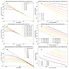 |
Fig. 1. Impact of adiabatic energy loss on the particle energy spectrum as described by Eq. (9). We set an initial flux spectrum with parameters j0 = 108[#/cm2/s/sr/MeV], γ = 4, and a constant solar wind speed of Vsw = 450 [km/s]. Panel a shows the peak flux spectrum at 1 AU for different diffusion coefficient indexs, α. Panel b shows the adiabatic energy loss of particles with a given initial energy corresponding to Panel a. Panel c shows the peak flux spectrum at 1 AU with different diffusion normalization coefficients, κ0. Panel d shows the adiabatic energy loss of particles with a given initial energy corresponding to Panel c. Panel e shows the evolution of the peak flux spectrum at different heliocentric distances. Panel f shows the adiabatic energy loss corresponding to Panel e. |
3. SEPEM dataset and methods
The Solar Energetic Particle Environment Modelling (SEPEM) project is a WWW interface to SEP data together with a range of modeling tools and functionalities intended to support space mission design1. The system provides an implementation of several well-known modeling methodologies, built upon cleansed datasets. A large number of datasets have been combined into an SQL database for convenient access. SEPEM also affords the user increased flexibility in their analysis and enables the generation of mission-integrated fluence statistics, peak flux statistics, and other functionalities. Additionally, it integrates effect tools that calculate single-event upset rates and radiation doses for a variety of scenarios; the statistical methods can further be applied to these effect parameters. In this work, we exploit the continuous and high-quality dataset and the long-term reference SEP event list to statistically study the properties of SEP spectra.
3.1. SEPEM dataset
The SEPEM reference proton dataset was originated from multiple spacecrafts and instruments2, such as Space Environment Monitor (SEM) and Energetic Particles Sensor (EPS) of Geostationary Operational Environmental Satellite (GOES), and the Goddard Medium Energy (GME) of Interplanetary Monitoring Platform 8 (IMP 8) satellite. The data were further processed through a process of correction, completion, cross-calibration, and energy rebinning (Crosby et al. 2015).
We selected the most up-to-date version (3rd version) of the SEPEM reference proton dataset for this study. This dataset includes proton flux data at 1AU with a time resolution of 5 minutes, spanning from July 1, 1974 to December 31, 2017. It also consists of 14 logarithmic energy bins ranging from 5 MeV to nearly 900 MeV, with a cosmic ray (CR) background subtraction. For each energy channel, we used the geometric mean of upper and lower limit as the effective energy (see Table 1).
Fourteen logarithmic energy bins of the third version of the SEPEM reference proton dataset.
We note that the uncertainty in the flux values is not provided in the SEPEM dataset and it is nontrivial to derive it as the flux is rebinned into energy bins different from those used directly for measurements. Since the resulting uncertainties on the fit parameters do not affect our subsequent analysis and results, we assigned an arbitrary uncertainty of 5% to all energy channels to complete the fitting algorithm, following previous studies (e.g., Dierckxsens et al. 2015).
3.2. SEPEM reference event list
At present, there is no world-wide consistent definition of the start and end time for SEP events. The SEPEM project selected 7.23–10.46 MeV proton channel as the reference channel and generated a reference SEP event list3 based on the following standards (Jiggens et al. 2011): (1) threshold for the start and end of an event: 0.01 [#/cm2/s/sr/MeV]; (2) minimum peak flux: 0.5 [#/cm2/s/sr/MeV] and (3) minimum event duration and dwell time: 24 h.
Figure 2 shows the entire SEPEM dataset used in this study (panel a), along with the corresponding daily Sunspot Number (SSN) for the same time period (panel b). The SSN data are accessed from the World Data Center SILSO4, Royal Observatory of Belgium, Brussels (SILSO World Data Center 2006-2022). As expected, more SEP events occur during periods of high solar activity. There are also quite a number of events occurring in the rising and decay phases of solar cycles. This is a well-known feature of SEP events and poses great challenges to the prediction of the occurrence and intensity of SEP events.
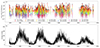 |
Fig. 2. Occurrence of SEP events is related to the solar activity cycle. Panel a shows the entire SEPEM dataset used in this study, namely the SEP proton flux-time profile from July 1, 1974 to December 31, 2017. Each vertical colored strip represents an SEP event, with different colors indicating various energy bins. Panel b shows the corresponding daily sunspot number (SSN) for the same time duration. The frequency of SEP events is positively correlated with SSN indicating solar activities. |
By the definition of single SEP event in the original SEPEM reference event list, there may be more than one enhancement from several events (namely, the “single” event can be further divided into several events with individual rising, peak, and declining phases). This could lead to an incorrect peak flux selection. Therefore, we modified the start and end times of the original SEPEM reference event list to make both the peak energy spectrum and integrated energy spectrum related to the same SEP event. More details can be found in Sect. 4 as well as Tables 3 and 4 (see Sect. Data availability).
3.3. Spectral fitting methods
Considering the forms of Eqs. (3) and (9), we utilize the nonlinear least squares method to obtain the optimal fitting parameters by minimizing the sum of squares error function, S(θ), with the following definition (Vugrin et al. 2007):
![Mathematical equation: $$ \begin{aligned} S(\boldsymbol{\theta }) = \sum _{i = 1}^{n}\left[f\left(\boldsymbol{\theta } ; \mathbf x _\mathbf{i }\right)-y_{i}\right]^{2}=\sum _{i = 1}^{n}\left[r_{i}(\boldsymbol{\theta })\right]^{2}, \end{aligned} $$](/articles/aa/full_html/2024/11/aa50046-24/aa50046-24-eq10.gif) (10)
(10)
where f(θ;xi) is the nonlinear model, θ is a vector of all parameters, and ri(θ) is residual.
Figure 3 shows an example of spectrum fitting. Panel a shows the flux time profile of a SEP event during November 1997. The black circles represent the peak flux of each energy bin. Panel b shows the peak flux spectrum fitting. Panel c shows the integrated fluence spectrum fitting throughout the event.
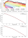 |
Fig. 3. Example of spectrum fitting. Panel a shows the flux time profile of a SEP event during November 1997. The black circles represent the peak flux of each energy bin. The vertical dashed lines indicated the start and end time for the integrated fluence spectrum. Panel b and c show the peak flux spectrum and the integrated fluence spectrum fitting, respectively. |
We note that there are still tens of events whose spectra can be fitted by neither Eq. (3) nor Eq. (9). There are multiple reasons for this, for instance, the possibility of a significant impact coming from the previous SEP event, influence of magnetic field structures on the SEP flux evolution, or other obvious instrumental or systematic errors. These events have been excluded from the table and the present study overall.
4. Results and discussion
Fitting parameters for the peak flux spectra following Eq. (9) are listed in Table 3 (see Sect. Data availability). As mentioned in Sect. 3.1, the uncertainties are calculated assuming a 5% arbitrary dataset uncertainty. Then, κ0_450 is calculated using a constant solar wind speed of 450 [km/s], while κ0 is calculated using the mean solar wind speed in the 6 days after the onset of the event. The corresponding solar wind speed values and standard deviations are listed in columns “Vsw” and “Vsw_err.” The solar wind speed data is obtained from GSFC/SPDF OMNIWeb interface5. We also obtained corresponding X-ray flare class for each SEP event from NOAA space environment services center6 for further analysis in Sect. 4.4.
The fitting parameters for the time-integrated fluence spectra, namely Eq. (3), are listed in Table 4 (see Sect. Data availability), where Ebreak = E0(γ1−γ2) is the transition energy of the Band function. The GLE event list is obtained from the Neutron Monitor GLE database7.
The calculation of the chi-square value for energy spectrum fitting is as follows:
![Mathematical equation: $$ \begin{aligned} \chi ^2=\frac{1}{N} \sum _{k = 1}^{N} \frac{\left[j_{\text{Fit}}\left(E_{k}\right)-j_{\text{Meas}}\left(E_{k}\right)\right]^{2}}{\sigma _{k}^{2}}, \end{aligned} $$](/articles/aa/full_html/2024/11/aa50046-24/aa50046-24-eq11.gif) (11)
(11)
where N is the number of energy bins, jFit(Ek) and jMeas(Ek) are the fitted and measured particle flux at the kinetic energy of Ek, respectively, and σk = 0.05jMeas(Ek) represents the aforementioned uncertainty on the data in the kth bin.
As we can see from Tables 3 and 4 (see Sect. Data availability), there are a significant number of events for which the value of χ2 is relatively large. The reasons for large χ2 value may be divided into two categories. One comes from the data processing algorithms. The data for SEP flux in the four highest energy channel of Table 1 can be significantly influenced by the GCR background-subtraction algorithms, which makes the fitting of this part difficult. The other reason is the influence of local acceleration and propagation effects, which are not considered in the model used here.
4.1. Distribution of the spectral parameters
We analyzed the peak flux spectra of 103 events and the integral fluence spectra of 164 events in total. The other 160(99) events listed in the reference event table are not involved in the analysis, as mentioned in Sect. 3.3.
The histograms in Fig. 4 show the distribution of fitting parameters listed in Tables 3 and 4 (see Sect. Data availability). Panel c illustrates the distribution of κ0_450 obtained through the utilization of a constant solar wind speed of 450 [km/s], and κ0 derived from real-time solar wind speed observations near Earth. Our subsequent analysis relies on the κ0 derived from real-time solar wind speed. The histograms show that the utilization of a constant solar wind speed does not appear to have a significant impact on the distribution of this parameter, but it may differ significantly for individual events as shown in Table 3 (see Sect. Data availability).
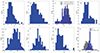 |
Fig. 4. Histograms of the fitting parameters shown in Tables 3 and 4. The results of the Anderson-Darling test are shown in Table 2, indicating that logC, γ1, and log E0 follow a normal distribution. |
To better quantify their distribution feature, we further investigated the distribution of fitting parameters using the Anderson-Darling test (Anderson & Darling 1954), with the results shown in Table 2. It can be seen that the statistical values of parameters logC, γ1, and log E0 are less than the critical value for a significance level of 0.05. This indicates that they mostly follow a normal distribution. A more detailed discussion is given in Sect. 5
Anderson-Darling test (significance level equals to 0.05) for the fitting parameters.
4.2. Relationships between the integral fluence spectra and peak flux spectra
We go on to try to find out whether the peak flux spectrum and integral fluence spectrum of the same SEP event have some kind of specific correlation. In Fig. 5, we demonstrate the relationships among the eight fitting parameters. For each SEP event indicated by a dot or circle, the four parameters of the peak flux spectrum (Eq. (9)) are plotted on the x-axes, while the four parameters of the integral fluence spectrum (Eq. (3)) are plotted on the y-axes. Solid dots are fitted parameters of GLE events, while the parameters of other SEP events are represented by hollow circles. The red line represents the linear regression curve of two parameters for both GLE events and non-GLE events, while the corresponding linear regression function is shown in the legend. The shaded area represents the confidence interval for one standard deviation. From the graph, we can summarize several interesting relationships among the two sets of parameters:
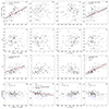 |
Fig. 5. Relationships among the eight fitting parameters. For each event, the four parameters of the peak flux spectrum (Eq. (9)) are plotted on the x-axes, while the four parameters of the integral fluence spectrum (Eq. (3)) are plotted on the y-axes. Solid dots are parameters of GLE events, while parameters of other SEP events are represented by hollow circles. In each panel where the R2 value is larger than 0.1, the red line represents the linear regression curve between two parameters for all events, and the corresponding linear regression function is shown in the legend. The shaded area represents the confidence interval for one standard deviation. The red dashed line in panel l represents the function of |γ2|=γ. |
– In panel a, the two normalization coefficients, C and j0, have a clear positive correlation. This is reasonable: if more SEPs are released at the source region, it is expected that a greater number of SEPs will be detected at Earth. Once the SEPs are released from the acceleration source, they will propagate in different directions. However, we only have data for the Earth’s orbit from the SEPEM dataset, which could result in the dispersion of this positive correlation.
– In panel d, the normalization coefficient C and the SEP source spectrum index, γ, also have a positive correlation, indicating that events with larger fluence at lower energy range more likely result from a softer SEP spectrum. There may be two reasons for this. One reason is that the SEPEM reference event list has a strict definition of SEP events (see Sect. 3.2) with the original intention to exclude particle enhancement events of non-solar origin from the list, such as those accelerated by stream interaction regions. However, this has resulted in some weaker SEP events also being excluded from the list. These events have a smaller normalization coefficients C and a larger spectrum index |γ| so that they do not have enough particles within the energy range of 7.23–10.46 MeV to define an SEP event in the SEPEM list. This may explain why there is no distribution of data points in the lower right part of this panel.
– Panel d also shows that there lack events with both very large intensities and small γ values. An early study by Fichtel & McDonald (1967) estimated that the total energy of particles in a large SEP event was about 1030[ergs], roughly 1 percent of total energy of a flare. Emslie et al. (2012) evaluated the energy budget of 38 large solar eruptive events between 2002 and 2006, and found that the SEP energy was between ∼0.1% and 3.5% of the total eruptive energy. For instance, they estimated that SEPs in GLE event Nr. 65 carried the highest energy of 4.3 × 1031[ergs], which was about 1.5% of the estimated free magnetic energy (∼3 × 1033[ergs]) of the X17 flare. The SEP spectrum is constrained by the total energy of accelerated particles:  . For a given energy limit, the larger the intensity scaling factor j0 (flux at 1 MeV), the steeper the spectrum (with a larger |γ|).
– In panel l, we can observe a strong positive correlation between the spectral indices of the high-energy portion of the integral spectra |γ2| and the initial spectra γ. We fit them as |γ2| = 0.67 × γ + 1.8. The results of linear regression is not far from the function of |γ2|=γ, which is represented by the red dashed line. This reason that |γ2| differs from γ for single events may be a result of the combined effects of adiabatic energy loss and multiple crossing effects related to particle scattering (Chollet et al. 2010). The former tends to result in a softer spectrum (|γ2|> γ) as higher-energy particles lose their energy to become lower-energy ones, while the latter modifies a spectrum to become harder (|γ2|< γ), since high-energy particles are more likely to be observed multiple times at a given location.
– Alternatively, the correlation between γ and γ1 as shown in panel h is less obvious. This is because lower energy particles experience more transport effects given their smaller mean-free path length (Lario et al. 2007). These effects include the aforementioned adiabatic energy loss and multiple crossing as well as cross-field diffusion and pitch angle scattering.
– Combining panel l and panel i, it can be observed that when there is an enhancement of particle acceleration in the SEP source region (i.e., larger j0), the SEP source spectrum tends to become softer (i.e., larger γ and |γ2|). This suggests that there might be some energy constraints in the process of SEP acceleration (as mentioned above) or that enhanced acceleration tends to prioritize the energization of low-energy particles as it takes longer time to accelerate particles to higher energies according to the diffusive shock acceleration mechanism (Decker & Vlahos 1986).
– The four panels at the bottom show the relationship between peak spectral parameters and the transition energy of the Band function: Ebreak = (γ1−γ2)E0. A larger diffusion coefficient power-law index α or a larger SEP event source energy spectrum index γ tends to result in a smaller transition energy. This indicates that the transition energy may be a result of the propagation process. Considering adiabatic cooling process which depends on κ and α, we have shown that the peak energy flux of the low-energy region is more significantly reduced with smaller α, as shown in panel a of Fig. 1. This results in a larger transition energy in the Band function.
– GLE events are registered when sufficient number of high-energy particles can overcome Earth’s magnetic shielding and generate secondary particles in Earth’s atmosphere to trigger ground neutron detectors. Thus, by definition, GLE spectra contain an enhanced high-energy component. This is shown in our plots: As marked by solid dots in each panel, GLE events typically have larger overall fluence normalization coefficients, C, harder SEP source spectra (smaller γ), as well as harder integral fluence spectra of the high-energy part (smaller |γ2|) and higher transition energies of the Band function.
4.3. Spectral evolution over the solar cycle
It has been almost 200 years since the discovery of the ∼11-year solar activity cycle (e.g., Hathaway 2015). As shown in Fig. 2, the occurrence of SEP events is closely related to the solar activity cycle. Due to the extensive coverage of the SEP event list studied in this work, which spans almost four solar cycles, it is possible to conduct statistical research on the energy spectra of SEP events during various solar activity phases.
Figure 6 demonstrates the time distribution of four parameters in the peak flux spectrum (Eq. (9)). Figure 7 demonstrates the time distribution of four parameters in the integral fluence spectrum (Eq. (3)). Solid dots are parameters of GLE events. The black lines in the background represent the daily sunspot number.
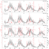 |
Fig. 6. Solar-cycle evolution of four parameters in the peak flux spectrum as shown by the left y-axes, namely, j0, α, κ0, and γ in Eq. (9) for panels a, b, c, and d, respectively. The uncertainty of each parameter results from assuming a 5% uncertainty in the SEPEM dataset as mentioned in Sect. 3.1. Solid dots are parameters of GLE events. The black lines in the background represent the daily sunspot number as scaled by the right y-axes. |
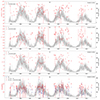 |
Fig. 7. Solar-cycle evolution of four parameters in the integral fluence spectrum in Eq. (3), as shown by the left y-axes. The uncertainty of each parameter results from assuming a 5% uncertainty in the SEPEM dataset as mentioned in Sect. 3.1. Solid dots are parameters of GLE events. The black lines in the background represent the daily sunspot number as scaled by the right y-axes. |
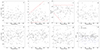 |
Fig. 8. Distribution of the energy spectrum parameters versus the sunspot number. We use the monthly averaged SSN centered at each SEP event’s start time. The red dashed lines illustrate the distribution boundaries of α and κ0 with respect to sunspot number. |
 |
Fig. 9. Solar-cycle dependent diffusion coefficient of different energies. Panel a shows the solar cycle evolution of the diffusion coefficient (left y-axis), which is defined by Eq. (6), for four different energies of protons (left legends). The gray lines in the background represent the daily sunspot number as scaled by the right y-axis. Panels b, c, d, and e show the diffusion coefficient distribution of 10, 50, 100, and 300 MeV protons, respectively. The distributions for low solar activity are represented by the dashed line, and for high solar activity are represented by the solid line. The median value of the diffusion coefficient, |

In Fig. 8, we examine the relationship between the energy spectral parameters and the sunspot number. Since the sunspot number is only a proxy for the solar activity and its daily values are highly fluctuating, we used the monthly averaged SSN centered at each SEP event’s start time, and we do not label the GLE event separately. The red dashed lines illustrate the distribution boundaries of α and κ0 with respect to sunspot number.
In Fig. 9, we further examine the diffusion coefficient evolution over the solar cycle. Panel a shows the results of the diffusion coefficient κ = κ0Eα calculated for protons of 1, 10, 100, and 300 MeV. We consider monthly-averaged SSN less than 70 as low solar activity periods and those greater than 200 as periods of high solar activity. The κ distributions of protons with different energies for the above two solar activities are compared in panels b, c, d, and e. We can see from Figures 6–9 that:
– The diffusion effect of SEPs is solar cycle-dependent. In Fig. 6(b),(c) and Fig. 8(b),(c), we can observe a weak solar cycle evolution of the fitted parameters, κ0 and α, which define the diffusion coefficient, κ. In Fig. 9, we can better see that during higher solar activity periods, both α and κ0 show a wider distribution: α can reach a larger magnitude than during solar maximum periods, while κ0 can reach smaller values compared to solar quiet periods. This suggests that the difference in the diffusion behavior of SEPs with different energies is larger during solar maximum periods.
– Figure 9 further illustrates the cycle-dependent diffusion coefficient of different energies (1, 10, 100, and 300 MeV protons in panels b,c,d,e, respectively). Both distribution and median value of diffusion coefficient indicate that low-energy particles (1 MeV, panel b) experience enhanced diffusion (smaller κ) during higher solar activities; high-energy particles (100 and 300 MeV, panels d and e), however, experience reduced diffusion during higher solar activities. This result agrees with the modeled results of the propagation of cosmic rays, as seen in Fig. 10 of Fiandrini et al. (2021) and Fig. 4 of Song et al. (2021). Quasi-linear theory (QLT) predicts that the two parameters α and κ0 are related to the power spectrum of the interplanetary magnetic field (IMF) turbulence. The power spectral index of the IMF turbulent level varies with different levels of solar activity, leading to changes in the scattering behavior of charged particles with different energies (Fiandrini et al. 2021).
– Other parameters, including j0, γ, C, γ1, γ2, and the break energy, do not show significant changes with varying sunspot numbers. This suggests that despite of the reduced occurring frequency, the SEP events during solar minimum are not necessarily weaker than those during solar maximum. Therefore, it is equally important to predict SEP events throughout different solar activity cycles.
4.4. Relationship with the X-ray flare class
Finally, we examine the relationship between the energy spectrum parameters of the SEP event and the peak X-ray flux8 of the corresponding flare. As shown in Fig. 10, the following conclusions can be drawn:
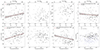 |
Fig. 10. Relationship between the energy spectrum parameters of the SEP event and the peak X-ray flux of the corresponding flare. Solid dots are parameters of GLE events, while parameters of other SEP events are represented by hollow circles. The red line represents the linear regression curve, and the corresponding linear regression equation is shown in the legend. The shaded area represents the confidence interval for one standard deviation. |
– There is a positive correlation between the normalization coefficient of energy spectrum and the peak X-ray flux (see Fig. 10(a) and (e)). This means that larger solar flares are usually accompanied by a greater flux of SEPs. This result is in agreement with previous studies (Belov et al. 2007; Kahler et al. 2007).
– The initial energy spectrum of SEPs, indicated by γ, and the spectrum of high-energy SEPs, indicated by γ2, are generally harder (see Fig. 10(d) and (h)) for larger solar flares. This suggests that stronger solar flares can produce more high-energy SEPs.
– The black solid dots representing the GLE event are distributed on the right side of all panels. This is an obvious result as these events usually correspond to solar flares of higher levels.
– As the peak X-ray flux increases, the other four parameters, α, κ0, γ1, and E0(γ1 − γ2), do not show a significant trend of change (see Fig. 10(b), (c), (f), and (h)). This may be because these four parameters are mainly related to the propagation effect of SEPs in space. Even though a strong solar flare event and associated CME could sometimes alter the characteristics of solar wind plasma in interplanetary space, these changes are typically the outcome of the propagating SEPs and can be observed later, that is, only after the SEP event (Gopalswamy et al. 2004).
5. Summary and discussion
Considering the effects of diffusion-dependent adiabatic cooling on SEPs propagation, we propose a modified power-law function (Eq. (9)) for the peak flux spectrum of SEP events. For the event-integrated spectrum, we utilized the widely accepted Band function (Eq. (3)) to extract information about particle distribution. Further employing the continuous and high-quality SEPEM dataset, we were able to study SEP events covering a period of 43 years for about four solar cycles from 1974 to 2018. Furthermore, we studied the peak spectrum and event-integrated spectrum for each event and fit them with the aforementioned functions to derive the fitting parameters that indicate the physical properties as well as the acceleration and transport mechanisms of SEPs.
We found that the propagation of SEPs in the inner solar system is slightly modulated by the level of solar activity, which is similar to the previous numerical research results on the propagation of cosmic rays (see Sect. 4.3). This helps us gain a better understanding of the propagation mechanism of charged particles in the interplanetary magnetic field.
To further investigate the acceleration mechanism of SEPs, we examined the relationship between the energy spectrum parameters of the SEP event and the peak X-ray flux of the corresponding flare. As shown in Sect. 4.4, we found that larger SEP events, such as GLE events characterized by higher particle flux, j0, and harder energy spectra (smaller γ), correspond to flares of a higher-level. The power-law relationship in Fig. 10 (panel a) is similar to that seen in other studies (e.g., Belov et al. 2007; Kahler et al. 2007). However, those works have used either the peak proton flux of a specific energy range or the integrated X-ray flux. This can be explained by big flare syndrome mechanism, namely: the statistically expected magnitude of measured flare energy manifestation is proportional to the energy released in a solar flare (Kahler 1982).
The reason for the double power-law characteristics of the SEP spectrum has not been clearly understood to this day. The understanding of transition energy or break energy is crucial for this topic. Based on the correlation between break energy and charge-to-mass ratio, several numerical simulation studies have suggested that the double power-law spectrum of SEP events may be directly generated by the acceleration at the shock (e.g., Mason et al. 2012; Desai et al. 2016; Yu et al. 2022). Alternatively, Mason et al. (2012) set the initial energy spectrum as a double power law and found that as particles propagate, the transition energy of the spectrum decreases. Other numerical studies have even suggested that the double power-law spectrum can be naturally built from an initial single power-law spectrum through particle propagation processes (e.g., Li & Lee 2015; Zhao et al. 2016).
By linking the peak flux spectrum which is closely related to the accelerated particle spectrum with the integral spectrum which contains more propagation effect, we can gain a better understanding of the acceleration and propagation behavior of particles. Based on the statistical analysis of 103 fitted SEP peak spectra and 164 fluence spectra, our study investigates the correlation between the transition energy of the double power-law spectrum and the particle diffusion coefficient (see Sect. 4.2). We note that the transition energy of the fitted Band function has a slight dependence on the diffusion coefficient, indicating that SEP propagation process can contribute to the formation and/or evolution of the double power law.
Moreover, as shown in Sect. 4.1, the three parameters in the Band function, logC, γ1, and log E0 approximately follow a normal distribution. We do not consider this to be a coincidence, but rather an indication that the physical processes determining these three parameters are different from the other parameters, such as α, κ0, and γ. Generally speaking, the time-integral energy spectrum can be considered as the superposition of a series of instantaneous energy spectra. During a single SEP event, the solar wind parameters in space can be approximated as constant, allowing the parameters of this series of instantaneous energy spectra to be considered to follow the same distribution. According to the central limit theorem, the superposition of these parameters with the same distribution will follow a normal distribution.
Overall, we outline the mechanism for establishing the double power-law spectrum of particle propagation process as follows. During the descending phase of the SEP event, particles collected by the detector may have traveled a much longer distance (including the multiple-crossing process) than the particles which arrived during the early phase due to the spatial propagation effect (Wang & Qin 2023). Thus, during the descending phase transport effects including adiabatic cooling could significantly impact the spectra of SEPs as shown by simulations (Qin et al. 2006; Mason et al. 2012). Since low-energy particles experience greater relative energy loss compared to high-energy particles, there would be more flattening of the energy spectrum in the low-energy region, resulting in a double power law.
Further analysis and attribution of SEP properties due to either flare- and CME-acceleration mechanisms would help us better understand and characterize the acceleration SEPs and improve the constraints set on them. Utilizing data collected at various solar distances (rather than just 1 AU) would contribute to a better understanding of the transport effects and the spatial evolution. To fully grasp the mechanisms behind SEP events, we require more comprehensive observation instruments that encompass a wider range of space, time, and energy.
Data availability
Tables 3 and 4 are available at https://doi.org/10.5281/zenodo.13270535.
Table 3 contains 16 columns for 103 SEP events and provides the following information: (Col. 1) Number of the current list. (Col. 2) Number in the SEPEM reference event list. (Cols. 3 and 4) SEP event start and end times in UTC. (Cols. 5 to 13) The parameters for the fitting of the SEP peak spectra, as outlined in Eq. (9), and their corresponding uncertainties. (Cols. 14 and 15) The real-time solar wind speed for Eq. (9) and its uncertainty. (Col. 16) The χ2 value for energy spectrum fitting.
Table 4 contains 17 columns for 164 SEP events and provides the following information: (Col. 1) Number of the current list. (Col. 2) Number in the SEPEM reference event list. (Cols. 3 and 4) SEP event start and end times in UTC. (Cols. 5 to 14) The parameters for the fitting of the SEP peak spectra, as outlined in Eq. (3), and their corresponding uncertainties. (Col. 15) Label for GLE events. (Col. 16) The corresponding X-ray flare class. (Col. 17) The χ2 value for energy spectrum fitting.
Solar Influences Data Analysis Center https://www.sidc.be/SILSO/datafiles
Obtained from https://www.swpc.noaa.gov/
Acknowledgments
The authors thank the anonymous reviewer for his/her time and effort in helping us improve this paper. The authors acknowledge the support by the Strategic Priority Program of the Chinese Academy of Sciences (Grant No. XDB41000000 and ZDBS-SSW-TLC00103), the National Natural Science Foundation of China (Grant Nos. 42188101, 42074222, 42130204). The authors also express their gratitude to the groups developing SEPEM project for the continuous and high-quality dataset and thank Dr. Piers Jiggens for his help in accessing the newest version of the SEPEM dataset.
References
- Anderson, T. W., & Darling, D. A. 1954, J. Am. Stat. Assoc., 49, 765 [Google Scholar]
- Band, D., Matteson, J., Ford, L., et al. 1993, ApJ, 413, 281 [Google Scholar]
- Belov, A., Kurt, V., Mavromichalaki, H., & Gerontidou, M. 2007, Sol. Phys., 246, 457 [NASA ADS] [CrossRef] [Google Scholar]
- Chollet, E., Giacalone, J., & Mewaldt, R. 2010, J. Geophys. Res.: Space Phys., 115, A6 [Google Scholar]
- Crosby, N., Heynderickx, D., Jiggens, P., et al. 2015, Space Weather, 13, 406 [CrossRef] [Google Scholar]
- Decker, R. B., & Vlahos, L. 1986, ApJ, 306, 710 [NASA ADS] [CrossRef] [Google Scholar]
- Desai, M. I., Mason, G. M., Dayeh, M. A., et al. 2016, ApJ, 816, 68 [NASA ADS] [CrossRef] [Google Scholar]
- Dierckxsens, M., Tziotziou, K., Dalla, S., et al. 2015, Sol. Phys., 290, 841 [CrossRef] [Google Scholar]
- Emslie, A., Dennis, B., Shih, A., et al. 2012, ApJ, 759, 71 [NASA ADS] [CrossRef] [Google Scholar]
- Fiandrini, E., Tomassetti, N., Bertucci, B., et al. 2021, Phys. Rev. D, 104, 023012 [NASA ADS] [CrossRef] [Google Scholar]
- Fichtel, C., & McDonald, F. 1967, ARA&A, 5, 351 [NASA ADS] [CrossRef] [Google Scholar]
- Forman, M., Ramaty, R., & Zweibel, E. 1986, Phys. Sun: Vol. II: Sol. Atmosp., 249 [Google Scholar]
- Fu, X., Lu, Q., & Wang, S. 2006, Phys. Plasmas, 13, 1 [Google Scholar]
- Gopalswamy, N., Yashiro, S., Krucker, S., Stenborg, G., & Howard, R. A. 2004, J. Geophys. Res.: Space Phys., 109, A12 [CrossRef] [Google Scholar]
- Guo, J., Wang, B., Whitman, K., et al. 2024, Adv. Space Res., in press, https://doi.org/10.1016/j.asr.2024.03.070 [Google Scholar]
- Hathaway, D. H. 2015, Liv. Rev. Sol. Phys., 12, 1 [CrossRef] [Google Scholar]
- Hollebeke, Van., & Ma Sung, M. 1975, Sol. Phys., 41, 189 [NASA ADS] [CrossRef] [Google Scholar]
- Jiggens, P. T., Gabriel, S. B., Heynderickx, D., et al. 2011, in 2011 12th European Conference on Radiation and Its Effects on Components and Systems, 549 [CrossRef] [Google Scholar]
- Jones, F. C., & Ellison, D. C. 1991, Space Sci. Rev., 58, 259 [Google Scholar]
- Kahler, S. 1982, J. Geophys. Res.: Space Phys., 87, 3439 [NASA ADS] [CrossRef] [Google Scholar]
- Kahler, S., Cliver, E., & Ling, A. 2007, J. Atmosp. Sol.-Terr. Phys., 69, 43 [NASA ADS] [CrossRef] [Google Scholar]
- Klein, K.-L., & Dalla, S. 2017, Space Sci. Rev., 212, 1107 [Google Scholar]
- Kurt, V., Logachev, I. I., Stolpovskii, V., & Daibog, E. 1981, Int. Cosmic Ray Conf., 3, 69 [NASA ADS] [Google Scholar]
- Lario, D., Aran, A., Agueda, N., & Sanahuja, B. 2007, Adv. Space Res., 40, 289 [Google Scholar]
- Li, G., & Lee, M. A. 2015, ApJ, 810, 82 [NASA ADS] [CrossRef] [Google Scholar]
- Mason, G. M. 2007, Space Sci. Rev., 130, 231 [Google Scholar]
- Mason, G., Li, G., Cohen, C., et al. 2012, ApJ, 761, 104 [NASA ADS] [CrossRef] [Google Scholar]
- McCracken, K., Rao, U., Bukata, R., & Keath, E. 1971, Sol. Phys., 18, 100 [NASA ADS] [CrossRef] [Google Scholar]
- Mewaldt, R. A., Cohen, C. M. S., Labrador, A. W., et al. 2005, J. Geophys. Res.: Space Phys., 110, A9 [NASA ADS] [CrossRef] [Google Scholar]
- Mewaldt, R., Looper, M., Cohen, C., et al. 2012, Space Sci. Rev., 171, 97 [NASA ADS] [CrossRef] [Google Scholar]
- Parker, E. N. 1963, Interplanetary Dynamical Processes (New York: Interscience Publishers) [Google Scholar]
- Parker, E. N. 1965, Planet. Space Sci., 13, 9 [Google Scholar]
- Qin, G., Zhang, M., & Dwyer, J. 2006, J. Geophys. Res.: Space Phys., 111, A8 [CrossRef] [Google Scholar]
- Raukunen, Osku., Vainio, Rami., Tylka, Allan J., et al. 2018, J. Space Weather Space Clim., 8, A04 [NASA ADS] [CrossRef] [EDP Sciences] [Google Scholar]
- Reames, D. V. 1999, Space Sci. Rev., 90, 413 [NASA ADS] [CrossRef] [Google Scholar]
- Reames, D. V. 2013, Space Sci. Rev., 175, 53 [CrossRef] [Google Scholar]
- SILSO World Data Center 2006-2022, International Sunspot Number Monthly Bulletin and online catalogue [Google Scholar]
- Song, X., Luo, X., Potgieter, M. S., Liu, X., & Geng, Z. 2021, ApJS, 257, 48 [NASA ADS] [CrossRef] [Google Scholar]
- Tylka, A. J. 2001, J. Geophys. Res.: Space Phys., 106, 25333 [NASA ADS] [CrossRef] [Google Scholar]
- Vugrin, K. W., Swiler, L. P., Roberts, R. M., Stucky-Mack, N. J., & Sullivan, S. P. 2007, Water Resour. Res., 43, 3 [CrossRef] [Google Scholar]
- Wang, Y., & Qin, G. 2023, The Astrophysical Journal, 954, 81 [NASA ADS] [CrossRef] [Google Scholar]
- Yu, F., Kong, X., Guo, F., et al. 2022, ApJ, 925, L13 [NASA ADS] [CrossRef] [Google Scholar]
- Zhao, L., Zhang, M., & Rassoul, H. K. 2016, ApJ, 821, 62 [Google Scholar]
All Tables
Fourteen logarithmic energy bins of the third version of the SEPEM reference proton dataset.
Anderson-Darling test (significance level equals to 0.05) for the fitting parameters.
All Figures
|
Fig. 1. Impact of adiabatic energy loss on the particle energy spectrum as described by Eq. (9). We set an initial flux spectrum with parameters j0 = 108[#/cm2/s/sr/MeV], γ = 4, and a constant solar wind speed of Vsw = 450 [km/s]. Panel a shows the peak flux spectrum at 1 AU for different diffusion coefficient indexs, α. Panel b shows the adiabatic energy loss of particles with a given initial energy corresponding to Panel a. Panel c shows the peak flux spectrum at 1 AU with different diffusion normalization coefficients, κ0. Panel d shows the adiabatic energy loss of particles with a given initial energy corresponding to Panel c. Panel e shows the evolution of the peak flux spectrum at different heliocentric distances. Panel f shows the adiabatic energy loss corresponding to Panel e. |
| In the text | |
|
Fig. 2. Occurrence of SEP events is related to the solar activity cycle. Panel a shows the entire SEPEM dataset used in this study, namely the SEP proton flux-time profile from July 1, 1974 to December 31, 2017. Each vertical colored strip represents an SEP event, with different colors indicating various energy bins. Panel b shows the corresponding daily sunspot number (SSN) for the same time duration. The frequency of SEP events is positively correlated with SSN indicating solar activities. |
| In the text | |
|
Fig. 3. Example of spectrum fitting. Panel a shows the flux time profile of a SEP event during November 1997. The black circles represent the peak flux of each energy bin. The vertical dashed lines indicated the start and end time for the integrated fluence spectrum. Panel b and c show the peak flux spectrum and the integrated fluence spectrum fitting, respectively. |
| In the text | |
|
Fig. 4. Histograms of the fitting parameters shown in Tables 3 and 4. The results of the Anderson-Darling test are shown in Table 2, indicating that logC, γ1, and log E0 follow a normal distribution. |
| In the text | |
|
Fig. 5. Relationships among the eight fitting parameters. For each event, the four parameters of the peak flux spectrum (Eq. (9)) are plotted on the x-axes, while the four parameters of the integral fluence spectrum (Eq. (3)) are plotted on the y-axes. Solid dots are parameters of GLE events, while parameters of other SEP events are represented by hollow circles. In each panel where the R2 value is larger than 0.1, the red line represents the linear regression curve between two parameters for all events, and the corresponding linear regression function is shown in the legend. The shaded area represents the confidence interval for one standard deviation. The red dashed line in panel l represents the function of |γ2|=γ. |
| In the text | |
|
Fig. 6. Solar-cycle evolution of four parameters in the peak flux spectrum as shown by the left y-axes, namely, j0, α, κ0, and γ in Eq. (9) for panels a, b, c, and d, respectively. The uncertainty of each parameter results from assuming a 5% uncertainty in the SEPEM dataset as mentioned in Sect. 3.1. Solid dots are parameters of GLE events. The black lines in the background represent the daily sunspot number as scaled by the right y-axes. |
| In the text | |
|
Fig. 7. Solar-cycle evolution of four parameters in the integral fluence spectrum in Eq. (3), as shown by the left y-axes. The uncertainty of each parameter results from assuming a 5% uncertainty in the SEPEM dataset as mentioned in Sect. 3.1. Solid dots are parameters of GLE events. The black lines in the background represent the daily sunspot number as scaled by the right y-axes. |
| In the text | |
|
Fig. 8. Distribution of the energy spectrum parameters versus the sunspot number. We use the monthly averaged SSN centered at each SEP event’s start time. The red dashed lines illustrate the distribution boundaries of α and κ0 with respect to sunspot number. |
| In the text | |
|
Fig. 9. Solar-cycle dependent diffusion coefficient of different energies. Panel a shows the solar cycle evolution of the diffusion coefficient (left y-axis), which is defined by Eq. (6), for four different energies of protons (left legends). The gray lines in the background represent the daily sunspot number as scaled by the right y-axis. Panels b, c, d, and e show the diffusion coefficient distribution of 10, 50, 100, and 300 MeV protons, respectively. The distributions for low solar activity are represented by the dashed line, and for high solar activity are represented by the solid line. The median value of the diffusion coefficient, |
| In the text | |
|
Fig. 10. Relationship between the energy spectrum parameters of the SEP event and the peak X-ray flux of the corresponding flare. Solid dots are parameters of GLE events, while parameters of other SEP events are represented by hollow circles. The red line represents the linear regression curve, and the corresponding linear regression equation is shown in the legend. The shaded area represents the confidence interval for one standard deviation. |
| In the text | |
Current usage metrics show cumulative count of Article Views (full-text article views including HTML views, PDF and ePub downloads, according to the available data) and Abstracts Views on Vision4Press platform.
Data correspond to usage on the plateform after 2015. The current usage metrics is available 48-96 hours after online publication and is updated daily on week days.
Initial download of the metrics may take a while.