| Issue |
A&A
Volume 695, March 2025
|
|
|---|---|---|
| Article Number | A25 | |
| Number of page(s) | 10 | |
| Section | The Sun and the Heliosphere | |
| DOI | https://doi.org/10.1051/0004-6361/202452591 | |
| Published online | 27 February 2025 | |
Radial dependence of solar energetic particle peak fluxes and fluences
Multispacecraft observations based on Parker Solar Probe, Solar Orbiter, and near-Earth particle detectors
1
Deep space Exploration Laboratory/School of Earth and Space Sciences, University of Science and Technology of China, Hefei, PR China
2
CAS Center for Excellence in Comparative Planetology, University of Science and Technology of China, Hefei 230026, China
⋆ Corresponding author; This email address is being protected from spambots. You need JavaScript enabled to view it.
Received:
12
October
2024
Accepted:
21
January
2025
Abstract
Context. We present a list of solar energetic particle (SEP) events detected by instruments on board the Solar and Heliospheric Observatory (SOHO), Parker Solar Probe (PSP), and Solar Orbiter between 2021 and 2023. The investigation focuses on identifying the peak flux and the fluence of SEP events in four energy ranges from 10.5 to 40 MeV, as observed by PSP or Solar Orbiter at heliospheric distances shorter than 1 AU and by SOHO at the Sun-Earth L1 Lagrangian point.
Aims. Based on the data from these events, we conduct a statistical analysis to study the radial dependence of the SEP proton peak flux and fluence at different energies.
Methods. We identified 42 SEP events with enhanced proton flux that were observed simultaneously by at least two out of three spacecraft (SOHO, PSP, and Solar Orbiter). These events were further selected based on a criterion of a difference smaller than a 30° difference in longitudinal separation between the magnetic footpoints of the two spacecraft. For the selected events, we used a linear interpolation method to compute the proton peak flux and fluence in four energy ranges and quantified their radial dependence as a function of Rα, where R is the radial distance of the observer from the Sun.
Results. The peak flux and fluence of the SEP events display the following radial dependence: The average values of α across all energies range between about −3.7 and −2 for the peak fluxes and between −2.7 and −1.4 for the fluences. We also obtained the energy dependence of |α|, which decreases with increasing energy. Additionally, based on theoretical functions, we find that the SEP source and transport parameters may have a significant impact on α(E), and the measurement-derived |α(E)| values and their distribution fall within the range of theoretical predictions.
Conclusions. (1) Despite the uncertainties arising from the low statistics and the longitudinal influence, the radial dependence of the peak flux agrees with the upper limit R−3 predicted by previous studies. (2) The radial dependence on the fluence R−2 tends to be weaker than the radial decay of the peak flux. (3) As the proton energy increases, the proton mean free path increases, and the adiabatic cooling effect modifies the proton energy. As a result, the peak flux and fluence decay more significantly with increasing radial distance for lower-energy particles.
Key words: Sun: activity / Sun: particle emission
© The Authors 2025
 Open Access article, published by EDP Sciences, under the terms of the Creative Commons Attribution License (https://creativecommons.org/licenses/by/4.0), which permits unrestricted use, distribution, and reproduction in any medium, provided the original work is properly cited.
This article is published in open access under the Subscribe to Open model. This email address is being protected from spambots. You need JavaScript enabled to view it. to support open access publication.
1. Introduction
Solar energetic particles (SEPs) are energetic particles that originated in processes associated with solar eruptions. They consist of protons, electrons, and ions. The typical energies range from suprathermal (a few keV) to relativistic (a few GeV) energies (Desai & Giacalone 2016). SEP events can last from a few hours to several days. SEP events, especially those with a high energy and intense flux, can impact electronic devices in space and pose radiation risks to human activities in space (e.g., Jun et al. 2024). Traditionally, SEP events have been categorized into impulsive and gradual types based on attributes such as their acceleration mechanism and the particle composition (Reames 1999; Klein & Dalla 2017). However, this classic perspective has been subject to considerable debate (e.g., Cohen et al. 1999; Cane et al. 2003, 2006; Cohen et al. 2021; Guo et al. 2024). A more comprehensive assessment of the spatial distribution of SEPs (longitudinal, radial, and latitudinal) would enhance our understanding of their characteristics.
Understanding of SEPs is also challenging because the physical mechanisms that drive the particle acceleration and transport within the heliosphere are two processes that are entangled in observations because they both influence the temporal evolution and the spatial distribution of SEPs as well as their energy dependence (e.g., Guo et al. 2024). Parker (1965) proposed using the Fokker-Planck equation to describe the particle transport in the heliosphere, which marked the beginning of particle transport theory. Many models were conducted based on this theory in the following decades to study the acceleration and/or propagation of SEPs (e.g., Heras et al. 1992, 1995; Dröge 1994; Kallenrode & Wibberenz 1997; Qin et al. 2006; Zhang et al. 2009; Dröge et al. 2010; Marsh et al. 2015; Hu et al. 2017; Zhang et al. 2023; Whitman et al. 2023). Most of these models were used to analyze SEP events and interpret the underlying physical mechanisms by probing the acceleration and transport theories under various conditions, such as the continuous injection of shock-accelerated particles or a changing magnetic connectivity of the observer to the shock front.
However, none of the current models can successfully explain all SEP events because the exact physical processes may differ from one event to the other (Whitman et al. 2023). In particular, the spatial distribution is determined by various factors related to the spatial extent of the particle sources, the interplanetary solar wind conditions through which particles propagate, the connectivity of the observer to the source, the duration of the particle injection, and the transport processes undergone by the particles. In most cases, none of these factors can be accurately derived from measurements, and they are often approximated as an ideal scenario, such as the assumption of the propagation path along the nominal Parker spiral determined via the in situ solar wind speed. Therefore, the analysis of SEP events based on observations by multiple observers at multiple heliospheric locations continues to play a critical role in advancing our understanding of the spatial distribution of SEPs, which is related to the acceleration and transport processes. The analysis of the distribution of SEP events in interplanetary space necessitates a comprehensive consideration of the longitudinal and radial transport. However, it is challenging to separate these two components.
For the longitudinal distributions of the SEP flux, Kahler (1982) employed the function Ip ∼ exp( − 1.604ΔΦ) to depict the longitudinal dependence of the SEP intensities observed by near-Earth spacecraft, where Ip represents the 20–40 MeV proton peak intensity and ΔΦ is the longitudinal difference between the flare and W50° (which is approximated as the best connection angle). In order to predict proton intensities at 1 AU that exceed 10 MeV, Balch (1999) employed a complex function that calculated the longitudinal separation between the observer’s magnetic footpoint and the flare site. This function can be approximated by a decrease of one order of magnitude for every 100° in longitude. Lario et al. (2006) used Helios and Interplanetary Monitoring Platform (IMP) satellite data to examine and analyze the longitudinal and radial dependences of energetic particle intensities during SEP events. In the past decade, the peak proton intensities observed by the Solar Terrestrial Relations Observatory (STEREO-A, STEREO-B) and the Advanced Composition Explorer (ACE) satellites at various energies were frequently fit to a Gaussian distribution to explore the longitudinal distribution of SEP events (Lario et al. 2013; Richardson et al. 2014; Xie et al. 2019).
For the radial dependence, Hamilton (1988) used the spherically symmetric transport model to study the radial dependence of the SEP peak flux. Lario et al. (2007) solved the focused-diffusion SEP transport equation for particle injection fixed at the Sun and modeled the radial dependence of 8.3 MeV and 34.6 MeV protons within 1 AU. The modeled radial dependence of the proton peak flux and fluence varies for different parameters, ranging from R−3 ∼ R−1.3 and R−1.5 ∼ R−0.7 respectively. Verkhoglyadova et al. (2012) later modeled the acceleration and transport of protons and iron ions at evolving coronal mass ejection shocks that propagate through the heliosphere, with a radial dependence of the peak flux ranging from R−2.9 ∼ R−1.8 in 0.3–5 MeV/n. Recently, Rodríguez-García et al. (2023) employed statistical models to examine the radial dependence of ∼200 keV electron peak fluxes of 61 electron events and their energy spectral index. Kollhoff et al. (2023) examined the radial dependence of the peak intensity of electron events, the maximum first-order anisotropy, the flux increase after the onset, and the time of the maximum flux within 15° between satellite nominal magnetic footpoints. Both studies concluded that the radial dependence of the peak intensities detected by spacecraft with small longitudinal separations approximates the relation R−3. This relation can also be inferred from the theoretical assumption that particle transport equations are predominantly governed by diffusion, as suggested by Vainio et al. (2007).
However, the radial dependence of the SEP peak flux and fluence in various energy ranges was not thoroughly investigated by previous studies. Currently, with new spacecraft data from the Parker Solar Probe (PSP) (Fox et al. 2016) and Solar Orbiter (Müller et al. 2020), which are traveling at inner heliospheric distances (less than 1 AU), we have an excellent chance to clarify and deepen our understanding of how SEP particles are distributed radially in the inner heliosphere. Our investigation is based on simultaneous SEP observations by two spacecraft at varying radial distances from the Sun, but located at close-by nominal interplanetary magnetic field (IMF) lines. In Sects. 2 and 3, we detail the datasets we used, the event selection criteria, and the analysis of the radial dependence of the peak flux and fluence in different energy ranges. Section 4 provides a summary and discussion of the findings.
2. SEP event selection criteria
We conducted an analysis of the data obtained from PSP, Solar Orbiter, and the Solar and Heliospheric Observatory (SOHO), which is located at the Sun-Earth L1 Lagrangian point from January 1, 2021 to January 1, 2024. Figure 1 illustrates the proton intensities measured by the three satellites during this period. We employed hourly averaged values of the particle intensities to improve the statistics of the data. The radial distance of SOHO from the Sun fluctuated between 0.97 and 1.01 AU. The radial distance of PSP ranged between about 0.05 AU and 0.78 AU, and that of Solar Orbiter varied between about 0.29 and 1.01 AU in this period, as shown by the brown curves (scaled by the right y-axes) in Fig. 1b and Fig. 1c, respectively. To minimize the uncertainties caused by the differing viewing perspectives of the energetic particle instruments on board the different satellites, we utilized data obtained from sunward-pointing instruments aboard three spacecraft: Energetic Particle Instruments High energy particle (EPIHi) on PSP (McComas et al. 2016), the High Energy Detector (HED) on Solar Orbiter (Müller et al. 2020), and both the Energetic and Relativistic Nuclei and Electron experiment (ERNE) and Electron Proton Helium Instrument (EPHIN) on SOHO (Torsti et al. 1995; Domingo et al. 1995). It is important to note that the SOHO satellite performs a roll maneuver approximately every three months, in which it switches its nominal roll angle between 0 and 180 degrees. This change in orientation affects the alignment of the energetic particle instruments relative to the IMF. The uncertainties introduced by the flip angle of SOHO are detailed in Sect. 4.
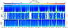 |
Fig. 1. Overview of multi-spacecraft observations of SEPs from January 2021 to January 2024. From top to bottom, we plot the hourly averages of (a) 4.3–7.8 MeV proton intensities measured by the EPHIN on board SOHO combined with 13–80 MeV proton intensities measured by the ERNE on board SOHO. (b) 8–64 MeV proton intensities measured by EPIHi on PSP. (c) 7.05–105 MeV proton intensities measured by HED on board Solar Orbiter. The radial distances of the PSP and Solar Orbiter spacecraft to the Sun are overplotted with orange lines and labeled in the right y-axes in panels (b) and (c), respectively. The magenta arrows in panel (a) indicate the 42 SEP events that were simultaneously observed by at least two of three observers (Earth, PSP, and Solar Orbiter). |
Based on the energetic proton observations by three observers during this period, we applied the following criteria to select SEP events for this study. (1) The event must be detected concurrently by at least two out of three spacecraft (SOHO, PSP, and Solar Orbiter) based on the flux between 10.5 and 15 MeV. A total of 42 SEP events were selected in this period and are marked in Figure 1. (2) The event must satisfy the condition that the footpoint longitude coordinate of nominal Parker spirals was within 30° for the two observers who saw the SEP event. (3) The event structure was to be simple during the rise and decay phases of the flux. Specifically, a singular SEP event was to occur within a brief period. Any SEP associated with local acceleration sources (i.e., interplanetary shocks) was to be distinctly identifiable and removed from the main event. (4) After applying items (2) and (3), we selected 22 of the 42 events and defined them as Group A in the following study. (5) We further selected events with a clear impulsive feature: For the energy range of 10.5-15 MeV, the peak was to be reached within 6 hours after the onset, and the peak flux was to be more than one order of magnitude greater than the background flux. This criterion left a total of 13 events (defined as Group B, which belongs to Group A).
Each of the 42 SEP events is indicated by a distinct magenta arrow in panel (a) of Figure 1. We collected information for 42 events, and this information is available for download1. For each event, we give the timing of coronal mass ejection (CME) eruptions as observed by the SOHO coronagraph imagers2, the timing of type II radio bursts from the e-Callisto solar spectrometer website3, the flare location and class sourced from the solar event website4, the roll angle of SOHO, the radial distance, longitude, and latitude value in Stonyhurst coordinates for three satellites from the Solar-Mach tool (Gieseler et al. 2023), the footpoint longitude coordinate of the nominal Parker spiral field line of each observer based on the observed in situ solar wind speed, and the peak flux and event-integrated fluence within different energy ranges for PSP, Solar Orbiter, and SOHO.
The satellite spatial distribution of the 13 events in Group B are shown in Fig. A.1, except for one event (March 21, 2022) that alone was observed by all three satellites with impulsive features. We therefore selected it as a case study and show the detailed calculation process in Fig. 2.
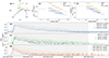 |
Fig. 2. Example of the event analysis. Panel (a) depicts the spatial distribution of the satellites in the heliospheric equatorial plane on March 21, 2022. Panels (b)–(d) illustrate the temporal evolution of the proton flux for three satellites in various energy ranges. Panels (e) and (f) present the spectra derived from the peak time of each energy and event-integrated period (shadow area in panels (b)–(d)), respectively. The light lines correspond to the original data sourced from mission websites, and the dark lines represent data that we interpolated to the four energy ranges defined in this analysis. |
3. Radial dependence analysis of SEP events
3.1. Data analysis
Assuming that particles primarily move along the nominal Parker spiral, we minimized the longitudinal diffusion effect when two spacecraft are located on the same IMF line or when two IMF lines have very small separation angles. In these situations, it is ideal to study the radial diffusion effect and the radial dependence of the SEP flux (e.g., Fu et al. 2022). However, two observers are located on the exact same IMF only very rarely.
To establish a reasonable longitudinal constraint for selecting events in this work, we refer to previous studies that used a Gaussian function exp[−(ϕ − ϕ0)2/2σ2] to model the longitudinal distribution of SEPs at 1AU, where ϕ is the longitudinal separation between the parent active region and the footpoint of the nominal IMF line connecting each spacecraft with the Sun, ϕ0 is the distribution centroid, and σ determines the distribution width. For instance, Lario et al. (2013) obtained σ = 43° ±2° for the 15–40 MeV and σ = 45° ±1° for the 25–53 MeV, while Richardson et al. (2014) reported σ = 43° ±13° for the 14–24 MeV. Based on a normal distribution with σ = 43°, we determined the ratio of the maximum to minimum values within any 30° interval of the Gaussian distribution. Within the full width at half maximum range, the ratio varied between 1.76 and 1.06. For a much more confined interval of 10° (with much fewer statistics), the ratio ranged between 1.27 and 1.01 (which is not a significant improvement in comparison). Consequently, we decided that < 30° is a good threshold to ensure an adequate number of events while minimizing the impact of longitudinal effects, thereby maintaining the focus of our study.
Following former studies (Lario et al. 2006), we calculated the radial dependence of the peak intensity and fluence by the exponential index α(E) over different energy ranges as
 (1)
(1)
where f1(E) and f2(E) are the proton intensities observed at the two spacecraft at the same energy E, and R1 and R2 are the corresponding radial distances of the two observers.
We analyzed the radial dependence of the peak flux and fluence measured by the SOHO and PSP or Solar Orbiter for the events in Group A (22 in total). To account for background fluxes, we defined the mean value of a pre-event period within one day before the onset time (lasting between 6 to 24 hours) as the background, and we calculated the peak flux and event fluence without this background. Ideally, it is critical for measurements from different instruments on board different spacecraft that the particle intensities are intercalibrated, as was done previously for near-Earth particle detectors (e.g., Lario et al. 2013). However, this is not feasible for the current study due to the spatial differences of PSP, Solar Orbiter, and Earth during all the commonly observed SEP events, as shown in Fig. 1. We discuss the possible effects on our results due to the lack of inter calibration in Sect. 4. Since different spacecraft have differently defined energy ranges, we first converted their fluxes into the same energy range before we applied the gradient calculation. To achieve this, we used a linear interpolation on the logarithmic energy bins of the raw data to obtain the flux in the four energy ranges defined in this study: 10.5–15 MeV, 15–20 MeV, 20–30 MeV, and 30–40 MeV. Then we used Eq. (1) to determine the radial dependence of the peak flux and fluence based on f1(E) and f2(E), which were derived from two observers at different radial distances.
Figure 2 shows the example of an event that occured on March 21, 2022. The magnetic footpoints backmapped to the solar surface for SOHO and Solar Orbiter have a difference as small as 6.8°, while the longitudinal difference between SOHO and PSP is about 100°, as shown in panel (a). Based on Earth remote-sensing observations, we found that the associated CME occurred on March 21, 2022 at 05:48:00 (SOHO/LASCO/C2) and the type II radio burst from 05:49 to 05:56, but the flare is rather weak; it was a class B4.5 event. Panels (b)–(d) display the temporal evolution of the proton flux with a 10-minute resolution. The peak flux is determined as the highest value (without the background value) in each energy bin. For events in Group B, such as the one shown here, the peak value is reached within 6 hours after the onset of the event. In contrast, for non-Group B events in Group A, the peak value is reached much later during the event. The fluence in each energy bin is determined as the integrated flux (without the pre-event background) from the onset time to the time when flux decays to the background value. The event duration we used to calculate the fluence may differ for different observers during the same event. For a few events, the occurrence of additional SEPs shortly before or after the event we studied can introduce biases in the fluence calculations. Specifically, if another prior SEP event occurred and was not fully concluded when the event of our focus commenced, the fluence might be underestimated if the background value were subtracted because the background was set to be fixed while it should have decayed with time. On the other hand, if the event flux had not returned to background levels prior to a subsequent event, the termination time for the fluence calculation must be moved forward, which also results in an underestimation of the fluence.
The gray region marked in panels (b)–(d) corresponds to the event duration, which is the same for the three observers in this event. Panels (e) and (f) illustrate the peak flux and fluence energy spectra without the background, respectively. The light color represents the data with the original energy bins sourced from the website5, and the darker color represents the interpolated flux in four energy ranges. The energy spectra at different locations all show a power-law shape, as shown in panels (e) and (f).
Figure 3 shows the dependence of the SEP proton peak flux (top panels) and fluence (bottom panels) as a function of the heliocentric distance in different energy ranges. The legend in each panel displays the mean (± the standard deviation) and the median (± median absolute deviation (MAD, Feigelson & Babu 2012)) of α(E) for the events, along with the number of the remaining events. Not all Group A (or Group B) events are shown in each panel because (a) extreme results (α < −10 or α > 0) were excluded (e.g., due to the small difference between R1 and R2) and (b) not all events reached the higher energy range(s) so that the event number decreased slightly with energy. The α values of some events significantly deviate from the statistical results, however. Several factors contribute to these deviations. One factor is that when two observers have very close radial distances (R1 ∼ R2), the estimate could have enlarged the uncertainty according to Eq. (1). Another possible explanation is that in some events, the solar wind disturbances might affect the SEP flux. Previous studies found that stream interaction regions and shock structures can modify the proton flux during SEP events (e.g., Guo et al. 2018). In addition, the longitudinal effect may still be influential, as illustrated in Fig. 6 and discussed in the corresponding text.
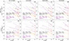 |
Fig. 3. Radial dependence of the peak flux and fluence of the selected SEP events measured by SOHO and PSP (or Solar Orbiter). Each line connects the same SEP event during which the longitudinal separation of the nominal Parker spirals of the two observers is < 30°. The upper four panels (a, b, c, and d) illustrate the radial dependence of the peak flux in four different energy ranges, respectively. The lower four panels depict the radial dependence of the fluence in four energy ranges, respectively. The red diamonds represent the proton intensity measured by SOHO, and the blue triangles and green circles represent the measurements by the Solar Orbiter and PSP satellites, respectively. Extreme results (α < −10 or α > 0) were excluded (92% events remain for each panel on average). All lines (purple and orange) represent the events in Group A (a total of 22 events) with the mean or median of the α values shown as the black legend. The purple lines highlight the impulsive SEP events observed by both observers, i.e., Group B (a total of 13 events), with the mean and median of the α values shown as the purple legend. More details can be found in the text. |
The radial dependence of the peak flux in the energy ranges studied here follows a relation within the range of R−3.7 ∼ R−2, with a discernible decreasing trend as the proton energy increases (|α(E)| reduces with E). For instance, the mean value of α for 10.5–15 MeV is −3.329, and the value for 30–40 MeV is −2.327. The median value is −2.999 and −2.026 for low and high energies, respectively. However, due to the limited statistics, this result is not statistically significant and falls within the uncertainty margin. In general, our results are consistent with previous results based on different observations and simulations with an upper limit of R−3 (Lario et al. 2006, 2007, 2013) and also with the theoretical predictions around R−3, as we discuss in more detail below.
The index of the radial dependence of the fluence shown in the bottom panels varies within the range of R−2.7 ∼ R−1.4, which is consistent with the result of R−2 based on the radial net flux derived from the time integration of the diffusion equation (Vainio et al. 2007). The general trend is also that |α(E)| reduces with increasing energy. However, the dependence is weaker than for the peak flux result, especially when the second energy bin in panel (f) is included.
3.2. Energy dependence of α
In interplanetary space, particle transport is primarily governed by various factors, including cross-field spatial diffusion, pitch-angle scattering, gradient or curvature drifts, magnetic focusing, and the adiabatic cooling term (Parker 1965; Bian & Li 2022). Each of these factors could influence the radial dependence of the proton intensities. Early theoretical work that considered a pure diffusion transport process (Hamilton 1988) predicted a radial dependence of R−3 for the peak flux attenuation as indicated by the dashed black lines in the top panels of Fig. 3. Our derived values of the radial dependence are between R−3.7 ∼ R−2, which indicates that the diffusion process may be a critical factor for the radial gradient. Other effects, such as pitch-angle scattering and magnetic focusing, may influence the SEP flux especially during events with high anisotropies. However, it is challenging to specify their impacts and their dependence on the radial distance among all other effects during an event. Strauss et al. (2020) employed numerical methods to investigate the impact of scattering and focusing process on the energy spectrum of energetic electrons. They also discussed the relation between the pitch-angle-related perpendicular or parallel mean free path for electrons and its variation with energy. Their results indicated that the peak flux of low-energy electrons (lower than 100 keV) is more weakly affected by these propagation effects and can effectively maintain the energy spectrum index of the injection source. Multiple studies have demonstrated that the mean free path of SEP protons exceeding 10 MeV is generally comparable to or even greater than that of electrons with energies below 100 keV (Dröge 2000; Palmer 1982). Consequently, protons and electrons in these energy ranges are expected to experience similar propagation effects.
Based on the proton peak spectrum model derived by Wang & Guo (2024), which incorporates radial diffusion and adiabatic cooling processes, we investigated the energy dependence of α(E) with the following steps. First, we assumed that the energy spectrum after acceleration follows a simple power-law,
 (2)
(2)
where f0 is a normalization coefficient in the same units as the particle flux f, γ is the index of the power-law energy spectrum after acceleration, Es is the source particle energy, and E0 is the normalization factor with a value of 1 MeV. At a solar distance r for protons with kinetic energy E, the peak flux f(r, E) can be determined by considering the diffusion effect during particle transport from the acceleration source as
![Mathematical equation: $$ \begin{aligned} f(r, E) = f_0 [(\frac{E}{E_0})^\beta + \frac{4}{9}\frac{V_{sw}}{\kappa _0}r]^{-\frac{\gamma }{\beta }}. \end{aligned} $$](/articles/aa/full_html/2025/03/aa52591-24/aa52591-24-eq3.gif) (3)
(3)
Here, Vsw denotes the solar wind speed, and κ0 is associated with the diffusion coefficient κ, which exhibits a power-law dependence on energy with an index of β:  .
.
By combining Eqs. (1) and (3), we derived the radial dependence of the peak flux as
![Mathematical equation: $$ \begin{aligned} \alpha (E) = -\frac{\gamma }{\beta }\frac{1}{\log (R_1/R_2)}[\log (1+C R_1)-\log (1+C R_2)], \end{aligned} $$](/articles/aa/full_html/2025/03/aa52591-24/aa52591-24-eq5.gif) (4)
(4)
where  .
.
Using typical values of κ0 = 1019 cm2/s (Wang & Guo 2024), Vsw = 400 km/s, R1 = 1 AU, and R2 = 0.6 AU, we derived from the above equation the relation between α(E) and β and γ for different energies, as shown in Fig. 4. The dashed white lines represent the mean value of α(E) plus/minus standard deviation, based on Group B data. The figure demonstrates that our measurement-derived values fall within the range of the theoretical predictions. Based on the study of over 100 events by Wang & Guo (2024), the parameters γ and β were found to typically distribute within the ranges of 2 to 7 and 0.5 to 5, respectively. Our calculations using κ0 values ranging from 1017 to 1020 cm2/s (see the animated version of Fig. 4) yielded γ varies between 2 and 8 and β ranges from 0.5 to 3, showing good agreement with the ranges reported by Wang & Guo (2024).
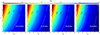 |
Fig. 4. Relation between α(E) (see the color bar at the top) for the peak flux and two parameters, γ (y-axis) and β (x-axis), in four different energy ranges shown in panels (a)–(d). The solid white line represents the mean value derived for Group B events, and the dashed white lines indicate the mean value plus and minus the standard deviation. The scaling factor of the diffusion parameter κ0 was fixed in this case to 1019 cm2/s. An animated version of this figure including results from different κ0 ranging from 1017 to 1020 cm2/s is available online. |
Fig. 4 clearly shows that the diffusion process of SEPs has a significant impact on α(E). A higher β value indicates that SEPs, especially those with higher energy, have a larger mean free path (MFP), and within a certain radial distance range [R2, R1], the probability of SEPs interacting with solar wind plasma is lower, resulting in a smaller α(E). Moreover, α(E) is also affected by the energy spectrum index γ of the SEP source. As a result of adiabatic cooling, particles of the same energy detected at radial positions R1 and R2 may have had a different initial energy Es in the source region. Specifically, given the same measured energy, a proton at R1 corresponds to a higher initial energy Es1 than a proton at R2, called Es2. In this case, α(E) also reflects the initial flux gradient (on a logarithmic scale) between Es1 and Es2, which equals the initial energy spectrum index γ, that is, a harder SEP source energy spectrum (smaller γ) results in a lower α(E).
To further investigate the relation between α(E) and energy, we calculated the derivative of Eq. (4) with respect to energy as
 (5)
(5)
This formula clearly indicates that given a source spectra and stable transport condition, the derivative of α(E) with respect to energy is always positive because R1 > R2. This result proves that as the energy increases, the value of α(E) also increases, and it ultimately approaches 0.
The theoretical prediction described above is consistent with our observational results, as shown earlier in Fig. 4. The energy dependence is further illustrated in Fig. 5, which presents the results calculated from Eq. (4). The figure shows a clear decrease in the radial dependence as the energy increases for the measurement and the modeled results. Our measurement-derived α(E) values fall well within the range of the model predictions, which are indicated by colored lines (derived from Eq. (4)) for each set of given solar wind and transport parameters.
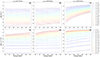 |
Fig. 5. Relation between α(E) (y-axis) for the peak flux and particle energy E(x-axis) with the evolution of the theoretical spectral and propagation parameters, γ, κ0, and β. Panels (a)–(c) explore the variations when β equals 1, while panels (d)–(f) present the results for γ at 3.75. In each panel, the pink diamonds represent the α within four energy ranges, derived from the mean value of Group B, and the error bars are the derived standard deviation. |
We note that the marked error bar of the measurement in Fig. 5 reflects not only the statistical uncertainty due to the limited number of events, but also the underlying physics process, which is different for each event. Specifically, the varying source information and diffusion coefficients that concurrently affect the values of α(E) differ from one event to the next. The assumption that the injection is impulsive and follows a single power law can be challenged. During the shock acceleration process, particles can be continuously accelerated at the shock front while it propagates outward. Consequently, the injection profile depends on the shock properties, which evolve in time and space, and on the connectivity of the observer to the shock front, which also changes over time (Heras et al. 1995; Pomoell et al. 2015). Moreover, the diffusion coefficient is expected to depend on time and space in reality (Chen et al. 2024), even during the same event. This variation was not considered in our simple model, however. Therefore, there may not be a unique solution for α(E), although studies with better statistics would be beneficial to advance our understanding.
4. Summary and discussion
This study examined a series of SEP events measured by SOHO and another satellite (either PSP or Solar Orbiter) within 1AU from January 2021 to January 2024. We identified 42 events during this period. For each SEP event, we identified the respective solar origin (flare size, location, CME outbreak, and type II radio burst time), estimated the nominal magnetic connection angle to the solar source, derived the peak intensity and fluence of the SEP protons, and provided statistical estimates of the radial dependence of the peak flux and fluence in four different energy ranges.
We focused on 22 of the 42 identified SEP events, defined as Group A, during which different observers had a close-by magnetic connection to the Sun (a footpoint separation smaller than 30°) such that the longitudinal difference was minimized at two observers. Furthermore, 13 out of these 22 events had an impulsive feature for both observers and were selected as Group B.
Following previous studies (Lario et al. 2006), we assumed that the radial dependence was represented as Rα. We confirm previous findings that for the peak flux, α fluctuates around -3, while for the event-integrated fluence, α is approximately -2. Generally, the results of |α| from Group A are slightly larger than those from Group B. The observed deviation in Group A is attributed to the inclusion of events whose flux progressively increased over time. This characteristic indicates that the satellite had a poor magnetic connectivity during the event, resulting in energetic particles that were transported to locations across the field lines due to longitudinal diffusion processes or that a time-dependent particle injection occurred at the shock front while it propagated outward (Reames 1999; Kallenrode 2003).
Figure 6 schematically illustrates how the magnetic connectivity may affect the measured radial dependence of the peak flux. In panel (a), both satellites are closely connected to the source of the SEP event (marked by the pink area, which represents the effective connection region) and detect the impulsive profile of the SEP flux, equivalent to the scenario of Group B. For pure diffusion transport process, the peak dependence satisfies |α|∼3. In panel (b), the inner observer (marked by the solid star at R2) is located outside the effective connection region and has a lower peak flux than in the region at the same radial distance (marked by the empty star). As a result, the derived radial gradient of two observers is smaller than expected. In panel (c), the outer observer (marked by the solid star at R1) is located outside the effective connection region, and the derived radial gradient is larger than expected. The events in Group A include all three scenarios, as illustrated in the figure. The distribution of |α| is therefore larger than in Group B.
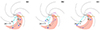 |
Fig. 6. Schematic illustrating how magnetic connectivity may affect the peak flux and α. Panels (a)–(c) depict three different connectivity scenarios. The red region represents the area in which SEP events can effectively reach the observer because the magnetic connectivity is good. The possible main acceleration sources of SEPs are CME shocks and flares, which are marked by the pink arc and gold arrow, respectively. The solid blue stars present the location of the observers, and the empty stars are the projected point of the observer from outside the red region to inside the region at the same radial distance. The expected radial dependence of the peak flux is |α|∼3, < 3, and > 3 for the three different panels. |
Previous studies attempted to first correct for the longitudinal effect when deriving the radial gradient of energetic particles. For instance, Rodríguez-García et al. (2023) used an empirical longitudinal-dependent function (Xie et al. 2019) to project the flux at different observers to the magnetic field line that was best connected to the solar flare and then calculated the radial effect. However, we investigated the energy dependence of the gradient, and the current longitudinal-dependent functions lack reliable energy-dependent information. Instead, we selected events with small separation angles (below 30°).
In particular, we obtained the energy dependence of α, showing a decreasing trend in |α| with increasing energy. Additionally, considering the energy spectrum of the proton peak flux under conditions of particle diffusion and adiabatic cooling, we derived the theoretical relation between α and the SEP source and the transport parameters, including γ, β, and κ0. These parameters all have a significant impact on α(E) and the measurement-derived |α(E)| values. Their distribution ranges are located within the range of the theoretical predictions.
Nevertheless, several instrumental effects might cause uncertainties in our results. One effect is that the high-gain antenna of the SOHO satellite has experienced structural issues since 2003, preventing it from rotating to transmit data to Earth. Therefore, it became necessary to periodically adjust the satellite Z-axis to orient the high-gain antenna toward Earth. This is typically done every three months. During this adjustment process, the ERNE viewing direction changes from being approximately parallel to perpendicular to the IMF (in the elliptic plane), which may affect the observed intensity. Second, a cross-calibration between different instruments remains pending in the current study, which might introduce systematic uncertainties into the results.
Currently, it is a challenge to quantitatively analyze the impact of the viewing angles on the peak flux for each SEP event. An approximate assessment of the effect of orientation on the peak flux of SOHO can be achieved by comparing it with other satellites that have multi-angle observations of high-energy particles. For instance, the HET detector on board Solar Orbiter has four directional probes. We therefore analyzed impulsive SEP events recorded by the Solar Orbiter from 2021 to 2024 at a radial distance larger than 0.8 AU. We computed the ratio of the peak intensities observed by the detectors oriented along the IMF toward the Sun relative to those oriented perpendicular to the IMF (i.e., toward north and south). The results revealed that this ratio diminishes as the energy increases. Because the statistical data are limited, we disregarded variations at different energies and computed the average value of the ratio within 10–40 MeV. We obtained the average ratio for Sun/North as 1.292 ± 0.423, and for Sun/South, it is 1.295 ± 0.354. Assuming that the flux observed in different directions perpendicular to IMF does not vary significantly, we employed an average value of 1.294 to adjust the SEP events following a 180-degree flip by SOHO. The final |α| values decrease by only a small factor of 14.42% and remain within the previously established confidence interval.
The cross-calibration between different particle detectors is often critical for ensuring the accuracy of the results. Previous studies investigated calibration factors between several satellites. For example, Xie et al. (2019) found that after conducting a comparative analysis of ACE and Wind data with STEREO measurements, the cross-calibration factor for ACE relative to STEREO was determined to be 1/1.4 for electrons in the energy range of 62–103 keV. Similarly, for protons in the energy range of 19–28 MeV, the cross-calibration factor for Wind relative to STEREO was found to be 1/1.5. Khoo et al. (2024) stated that for protons with an energy of 29 MeV, the flux measured by BepiColombo was approximately 35% lower than that measured by PSP. Carver et al. (2018) conducted a cross-calibration analysis between Global Positioning System (GPS) and Geostationary Operational Environmental Satellite (GOES). For proton fluxes with energies greater than 10 MeV, 20 MeV, 30 MeV, 60 MeV, and 100 MeV, the median ratio of GPS to GOES was 0.90, 0.90, 1.04, 1.24, and 1.07, respectively. However, an intercalibration of SOHO, PSP, and Solar Orbiter is challenging because no SEP events have been observed simultaneously by any two of these three satellites at the same location. Referring to previous studies, we assumed a 50% flux difference to quantify the influence on our results. Subsequently, we performed all the analyses based on the same event list and found that the mean values of α may differ by up to 25% for Group A events and by up to 30% for Group B. Future cross-calibration campaigns during close encounters of different spacecraft will be helpful to better quantify our results.
The assumption that the radial dependence of the SEP events is constant with distance as described in Eq. (1) can be challenged. As shown in Eq. (4), gradient α should also depend on R1 and R2. However, with the limited observations so far (based on only two observers in most cases), we cannot yet verify this prediction from existing measurements. Ideally, with at least three observers located within the pink region plotted in Fig. 6a, we can probe the dependence of α on R.
As the solar activity increases, we will be able to study the spatial distribution of intense SEP events with better statistics to better quantify the gradient and longitudinal distribution of SEPs in the heliosphere and perhaps to distinguish the longitudinal diffusion and radial diffusion effects. Future endeavors may involve using more satellites located near 1 AU as benchmarks, performing cross-calibration during close encounters of different spacecraft, and even studying the latitudinal distribution of SEPs. Additionally, we need to carry out further investigation using ongoing measurements as well as future missions, even those dedicated to exploring the planetary environment.
Data availability
Movie associated to Fig. 4 is available at https://www.aanda.org
The authors used the data from SOHO, PSP and Solar Orbiter instrument teams, and all the data used in this study is available at the website of NASA (https://cdaweb.gsfc.nasa.gov/). We summarized information for 42 events available for download here (https://doi.org/10.5281/zenodo.14699287)
Acknowledgments
The authors thank the anonymous reviewer for his/her time and effort in helping us to improve this article. The authors acknowledge the support by the National Natural Science Foundation of China (Grant Nos. 42188101, 42130204, 42474221).
References
- Balch, C. C. 1999, Radiat. Meas., 30, 231 [NASA ADS] [CrossRef] [Google Scholar]
- Bian, N., & Li, G. 2022, ApJ, 924, 120 [NASA ADS] [CrossRef] [Google Scholar]
- Cane, H. v., Von Rosenvinge, T., Cohen, C., & Mewaldt, R. 2003, GeoRL, 30, 12 [NASA ADS] [Google Scholar]
- Cane, H., Mewaldt, R., Cohen, C., & Von Rosenvinge, T. 2006, JGR. Space Phys., 111, A06S90 [NASA ADS] [Google Scholar]
- Carver, M. R., Sullivan, J. P., Morley, S. K., & Rodriguez, J. V. 2018, Space Weather, 16, 273 [NASA ADS] [CrossRef] [Google Scholar]
- Chen, X., Giacalone, J., Guo, F., & Klein, K. G. 2024, ApJ, 965, 61 [NASA ADS] [CrossRef] [Google Scholar]
- Cohen, C., Mewaldt, R., Leske, R., et al. 1999, GeoRL., 26, 2697 [NASA ADS] [Google Scholar]
- Cohen, C. M., Li, G., Mason, G. M., Shih, A. Y., & Wang, L. 2021, Solar physics and solar wind, 133 [CrossRef] [Google Scholar]
- Desai, M., & Giacalone, J. 2016, Liv. Rev. Sol. Phys., 13, 3 [NASA ADS] [CrossRef] [Google Scholar]
- Domingo, V., Fleck, B., & Poland, A. I. 1995, SoPh., 162, 1 [NASA ADS] [Google Scholar]
- Dröge, W. 1994, International Astronomical Union Colloquium (Cambridge University Press), 142, 567 [CrossRef] [Google Scholar]
- Dröge, W. 2000, ApJ, 537, 1073 [CrossRef] [Google Scholar]
- Dröge, W., Kartavykh, Y., Klecker, B., & Kovaltsov, G. 2010, ApJ, 709, 912 [CrossRef] [Google Scholar]
- Feigelson, E. D., & Babu, G. J. 2012, ArXiv e-prints [arXiv:1205.2064] [Google Scholar]
- Fox, N., Velli, M., Bale, S., et al. 2016, SSRv., 204, 7 [NASA ADS] [Google Scholar]
- Fu, S., Ding, Z., Zhang, Y., et al. 2022, ApJ, 934, L15 [NASA ADS] [CrossRef] [Google Scholar]
- Gieseler, J., Dresing, N., Palmroos, C., et al. 2023, FrASS, 9, 1058810 [Google Scholar]
- Guo, J., Dumbović, M., Wimmer-Schweingruber, R. F., et al. 2018, Space Weather, 16, 1156 [NASA ADS] [CrossRef] [Google Scholar]
- Guo, J., Wang, B., Whitman, K., et al. 2024, Adv. Space Res, 63, 3761 [Google Scholar]
- Hamilton, D. C. 1988, Jet Propulsion Lab., California Inst. of Tech., Interplanetary Particle Environment. Proceedings of a Conference [Google Scholar]
- Heras, A., Sanahuja, B., Smith, Z., Detman, T., & Dryer, M. 1992, ApJ, 391, 359 [NASA ADS] [CrossRef] [Google Scholar]
- Heras, A. M., Sanahuja, B., Lario, D., et al. 1995, ApJ, 445, 497 [NASA ADS] [CrossRef] [Google Scholar]
- Hu, J., Li, G., Ao, X., Zank, G. P., & Verkhoglyadova, O. 2017, JGR. Space Phys., 122, 10 [Google Scholar]
- Jun, I., Garrett, H., Kim, W., et al. 2024, Adv. Space Res, submitted [Google Scholar]
- Kahler, S. 1982, JGR. Space Phys., 87, 3439 [NASA ADS] [Google Scholar]
- Kallenrode, M. 2003, J. Phys. G: Nucl. Part. Phys., 29, 965 [NASA ADS] [CrossRef] [Google Scholar]
- Kallenrode, M.-B., & Wibberenz, G. 1997, JGR. Space Phys., 102, 22311 [Google Scholar]
- Khoo, L., Sánchez-Cano, B., Lee, C., et al. 2024, ApJ, 963, 107 [NASA ADS] [CrossRef] [Google Scholar]
- Klein, K.-L., & Dalla, S. 2017, SSRv., 212, 1107 [NASA ADS] [Google Scholar]
- Kollhoff, A., Berger, L., Brüdern, M., et al. 2023, A&A, 675, A155 [NASA ADS] [CrossRef] [EDP Sciences] [Google Scholar]
- Lario, D., Kallenrode, M.-B., Decker, R., et al. 2006, ApJ, 653, 1531 [NASA ADS] [CrossRef] [Google Scholar]
- Lario, D., Aran, A., Agueda, N., & Sanahuja, B. 2007, Adv. Space Res., 40, 289 [Google Scholar]
- Lario, D., Aran, A., Gómez-Herrero, R., et al. 2013, ApJ, 767, 41 [CrossRef] [Google Scholar]
- Marsh, M., Dalla, S., Dierckxsens, M., Laitinen, T., & Crosby, N. 2015, Space Weather, 13, 386 [CrossRef] [Google Scholar]
- McComas, D., Alexander, N., Angold, N., et al. 2016, SSRv., 204, 187 [NASA ADS] [Google Scholar]
- Müller, D., Cyr, O. S., Zouganelis, I., et al. 2020, A&A, 642, A1 [NASA ADS] [CrossRef] [EDP Sciences] [Google Scholar]
- Palmer, I. 1982, Rev. Geophys., 20, 335 [NASA ADS] [CrossRef] [Google Scholar]
- Parker, E. N. 1965, Planet. Space Sci., 13, 9 [Google Scholar]
- Pomoell, J., Aran, A., Jacobs, C., et al. 2015, J. Space Weather Space Clim., 5, A12 [NASA ADS] [CrossRef] [EDP Sciences] [Google Scholar]
- Qin, G., Zhang, M., & Dwyer, J. R. 2006, JGR. Space Phys., 111, A08101 [NASA ADS] [Google Scholar]
- Reames, D. V. 1999, SSRv., 90, 413 [NASA ADS] [Google Scholar]
- Richardson, I., Von Rosenvinge, T., Cane, H., et al. 2014, Coronal magnetometry, 437 [CrossRef] [Google Scholar]
- Rodríguez-García, L., Gómez-Herrero, R., Dresing, N., et al. 2023, A&A, 670, A51 [NASA ADS] [CrossRef] [EDP Sciences] [Google Scholar]
- Strauss, R. D., Dresing, N., Kollhoff, A., & Brüdern, M. 2020, ApJ, 897, 24 [NASA ADS] [CrossRef] [Google Scholar]
- Torsti, J., Valtonen, E., Lumme, M., et al. 1995, SoPh., 162, 505 [NASA ADS] [Google Scholar]
- Vainio, R., Agueda, N., Aran, A., & Lario, D. 2007, Space Weather: Research Towards Applications in Europe, 27 [NASA ADS] [CrossRef] [Google Scholar]
- Verkhoglyadova, O., Li, G., Ao, X., & Zank, G. 2012, ApJ, 757, 75 [NASA ADS] [CrossRef] [Google Scholar]
- Wang, Y., & Guo, J. 2024, A&A, 691, A54 [NASA ADS] [CrossRef] [EDP Sciences] [Google Scholar]
- Whitman, K., Egeland, R., Richardson, I. G., et al. 2023, Adv. Space Res., 72, 5161 [NASA ADS] [CrossRef] [Google Scholar]
- Xie, H., St. Cyr, O. C., Mäkelä, P., & Gopalswamy, N. 2019, JGR. Space Phys., 124, 6384 [NASA ADS] [CrossRef] [Google Scholar]
- Zhang, M., Qin, G., & Rassoul, H. 2009, ApJ, 692, 109 [NASA ADS] [CrossRef] [Google Scholar]
- Zhang, M., Cheng, L., Zhang, J., et al. 2023, ApJS, 266, 35 [NASA ADS] [CrossRef] [Google Scholar]
Appendix A: Additional figure
Figure A.1 depicts the satellite spatial distribution in the equatorial plane with different lines representing the nominal Parker spirals for SOHO (blue), PSP (green) and Solar Orbiter (orange).
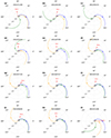 |
Fig. A.1. Illustration of various satellites spatial distribution (in the equatorial plane of the Stonyhurst coordinate system, with the Earth always corresponding to 0° longitude) during the onset of each SEP event in Group B (except for one event shown in Fig. 2). Observers marked by stars have seen the arrival of energetic protons, while those marked by an empty circle did not observe the SEPs. Different colors symbolize the nominal Parker spirals for SOHO (blue), PSP (green) and Solar Orbiter (orange). In each panel, the red arrow indicates the longitude of the flare. The flare direction is not certain in panel (l) and the flare is not observed from Earth in panel (c). |
All Figures
|
Fig. 1. Overview of multi-spacecraft observations of SEPs from January 2021 to January 2024. From top to bottom, we plot the hourly averages of (a) 4.3–7.8 MeV proton intensities measured by the EPHIN on board SOHO combined with 13–80 MeV proton intensities measured by the ERNE on board SOHO. (b) 8–64 MeV proton intensities measured by EPIHi on PSP. (c) 7.05–105 MeV proton intensities measured by HED on board Solar Orbiter. The radial distances of the PSP and Solar Orbiter spacecraft to the Sun are overplotted with orange lines and labeled in the right y-axes in panels (b) and (c), respectively. The magenta arrows in panel (a) indicate the 42 SEP events that were simultaneously observed by at least two of three observers (Earth, PSP, and Solar Orbiter). |
| In the text | |
|
Fig. 2. Example of the event analysis. Panel (a) depicts the spatial distribution of the satellites in the heliospheric equatorial plane on March 21, 2022. Panels (b)–(d) illustrate the temporal evolution of the proton flux for three satellites in various energy ranges. Panels (e) and (f) present the spectra derived from the peak time of each energy and event-integrated period (shadow area in panels (b)–(d)), respectively. The light lines correspond to the original data sourced from mission websites, and the dark lines represent data that we interpolated to the four energy ranges defined in this analysis. |
| In the text | |
|
Fig. 3. Radial dependence of the peak flux and fluence of the selected SEP events measured by SOHO and PSP (or Solar Orbiter). Each line connects the same SEP event during which the longitudinal separation of the nominal Parker spirals of the two observers is < 30°. The upper four panels (a, b, c, and d) illustrate the radial dependence of the peak flux in four different energy ranges, respectively. The lower four panels depict the radial dependence of the fluence in four energy ranges, respectively. The red diamonds represent the proton intensity measured by SOHO, and the blue triangles and green circles represent the measurements by the Solar Orbiter and PSP satellites, respectively. Extreme results (α < −10 or α > 0) were excluded (92% events remain for each panel on average). All lines (purple and orange) represent the events in Group A (a total of 22 events) with the mean or median of the α values shown as the black legend. The purple lines highlight the impulsive SEP events observed by both observers, i.e., Group B (a total of 13 events), with the mean and median of the α values shown as the purple legend. More details can be found in the text. |
| In the text | |
|
Fig. 4. Relation between α(E) (see the color bar at the top) for the peak flux and two parameters, γ (y-axis) and β (x-axis), in four different energy ranges shown in panels (a)–(d). The solid white line represents the mean value derived for Group B events, and the dashed white lines indicate the mean value plus and minus the standard deviation. The scaling factor of the diffusion parameter κ0 was fixed in this case to 1019 cm2/s. An animated version of this figure including results from different κ0 ranging from 1017 to 1020 cm2/s is available online. |
| In the text | |
|
Fig. 5. Relation between α(E) (y-axis) for the peak flux and particle energy E(x-axis) with the evolution of the theoretical spectral and propagation parameters, γ, κ0, and β. Panels (a)–(c) explore the variations when β equals 1, while panels (d)–(f) present the results for γ at 3.75. In each panel, the pink diamonds represent the α within four energy ranges, derived from the mean value of Group B, and the error bars are the derived standard deviation. |
| In the text | |
|
Fig. 6. Schematic illustrating how magnetic connectivity may affect the peak flux and α. Panels (a)–(c) depict three different connectivity scenarios. The red region represents the area in which SEP events can effectively reach the observer because the magnetic connectivity is good. The possible main acceleration sources of SEPs are CME shocks and flares, which are marked by the pink arc and gold arrow, respectively. The solid blue stars present the location of the observers, and the empty stars are the projected point of the observer from outside the red region to inside the region at the same radial distance. The expected radial dependence of the peak flux is |α|∼3, < 3, and > 3 for the three different panels. |
| In the text | |
|
Fig. A.1. Illustration of various satellites spatial distribution (in the equatorial plane of the Stonyhurst coordinate system, with the Earth always corresponding to 0° longitude) during the onset of each SEP event in Group B (except for one event shown in Fig. 2). Observers marked by stars have seen the arrival of energetic protons, while those marked by an empty circle did not observe the SEPs. Different colors symbolize the nominal Parker spirals for SOHO (blue), PSP (green) and Solar Orbiter (orange). In each panel, the red arrow indicates the longitude of the flare. The flare direction is not certain in panel (l) and the flare is not observed from Earth in panel (c). |
| In the text | |
Current usage metrics show cumulative count of Article Views (full-text article views including HTML views, PDF and ePub downloads, according to the available data) and Abstracts Views on Vision4Press platform.
Data correspond to usage on the plateform after 2015. The current usage metrics is available 48-96 hours after online publication and is updated daily on week days.
Initial download of the metrics may take a while.