| Issue |
A&A
Volume 691, November 2024
|
|
|---|---|---|
| Article Number | A8 | |
| Number of page(s) | 20 | |
| Section | Planets and planetary systems | |
| DOI | https://doi.org/10.1051/0004-6361/202449569 | |
| Published online | 25 October 2024 | |
No evidence for interstellar fireballs in the CNEOS database
1
Astronomical Institute, Slovak Academy of Sciences,
Dubravska cesta 9,
84504
Bratislava,
Slovakia
2
Institute of Applied Physics & Oeschger Center for Climate Change Research, Microwave Physics, University of Bern,
Bern,
Switzerland
3
Istituto Nazionale di Astrofisica, Osservatorio Astrofisico di Torino,
Via Osservatorio 20,
Pino Torinese
10025,
Italy
4
Università degli Studi di Torino – Dipartimento di Fisica,
Via Pietro Giuria 1,
Torino,
TO,
Italy
5
Astronomical Institute of the Czech Academy of Sciences,
Fricova 298,
25165
Ondřejov,
Czech Republic
6
IMCCE, Observatoire de Paris – PSL,
Denfert Rochereau, Bat. A.,
75014
Paris,
France
7
Institute for Particle Physics and Astrophysics, ETH,
Zürich,
Switzerland
8
Department of Physics, Astronomy and Geosciences, Towson University,
Towson,
MD,
USA
9
School of Earth and Space Exploration, Arizona State University,
Tempe,
AZ,
USA
★ Corresponding author; This email address is being protected from spambots. You need JavaScript enabled to view it.
, This email address is being protected from spambots. You need JavaScript enabled to view it.
, This email address is being protected from spambots. You need JavaScript enabled to view it.
Received:
10
February
2024
Accepted:
9
September
2024
Abstract
Context. The detection of interstellar meteors, especially meteorite-dropping meteoroids, would be transformative, as this would enable direct sampling of material from other stellar systems on Earth. One candidate is the fireball observed by U.S. government sensors on January 8, 2014. It has been claimed that fragments of this meteoroid have been recovered from the ocean floor near Papua New Guinea and that they support an extrasolar origin. Based on its parameters reported in the Center for Near Earth Object Studies (CNEOS) catalog, the fireball exhibits a hyperbolic excess velocity that indicates an interstellar origin; however, the catalog does not report parameter uncertainties.
Aims. To achieve a clear confirmation of the fireball’s interstellar origin, we assessed the underlying error distributions of the catalog data. Our aim was also to confirm whether the fragments of this meteoroid survived passage through the atmosphere and assess all conditions needed to unambiguously determine the fragments’ origin.
Methods. We approached the investigation of the entire catalog using statistical analyses and modeling, and we provide a comprehensive analysis of the individual hyperbolic CNEOS cases.
Results. We have developed several independent arguments indicating substantial uncertainties in the velocity and radiant position of the CNEOS events. We determined that all the hyperbolic fireballs exhibit significant deviations from the majority of the events in one of their velocity components, and we show that such mismeasurements can produce spurious parameters. According to our estimation of the speed measurement uncertainty for the catalog, we found that it is highly probable that such a catalog containing only Sun-bound meteors would show at least one event that appears highly unlikely to be Sun-bound. We also establish that it is unlikely that any fragments from a fireball traveling at the high inferred velocities could survive passage through the atmosphere. When assuming a much lower velocity, some fragments of this meteoroid could survive; however, they would be of a common Solar System origin and thus highly probable to be indistinguishable from the quantity of other local micrometeorites that have gradually accumulated on the sea floor.
Conclusions. We conclude that there is no evidence in the CNEOS data to confirm or reject the interstellar origin of any of the nominally hyperbolic fireballs in the CNEOS catalog. Therefore, the claim of an interstellar origin for the fireball recorded over Papua New Guinea in 2014 remains unsubstantiated. We have also gathered arguments that refute the claim that the collected spherules from the sea floor originated in the body of this fireball.
Key words: catalogs / meteorites, meteors, meteoroids
© The Authors 2024
 Open Access article, published by EDP Sciences, under the terms of the Creative Commons Attribution License (https://creativecommons.org/licenses/by/4.0), which permits unrestricted use, distribution, and reproduction in any medium, provided the original work is properly cited.
This article is published in open access under the Subscribe to Open model. This email address is being protected from spambots. You need JavaScript enabled to view it. to support open access publication.
1 Introduction
The Solar System continuously ejects cometary dust particles due to solar radiation pressure force after outgassing and the breakup of comets (Zook & Berg 1975; Moorhead 2021; Wehry & Mann 1999; Sommer 2023). Larger “rocks” are also accelerated into hyperbolic orbits due to the gravitational slingshot effect - one in about 10 000 from the Solar System are expected to be ejected Wiegert (2014). Just like the Solar System, other planetary systems continuously eject material into interstellar space, and this material may travel to the Solar System (Murray et al. 2004; Gregg & Wiegert 2023). Detecting such interstellar material and distinguishing it from interplanetary matter is exceedingly demanding, especially for particles observed as meteors (Hajduková 1994; Weryk & Brown 2004; Musci et al. 2012; Wiegert 2014; Hajduková et al. 2019; Vaubaillon 2022; Brown & Borovička 2023). A coherent picture of the full-size distribution of interstellar particles in the Solar System has not yet been established (Hajduková et al. 2020).
In this paper, we examine the likelihood that the first interstellar fireball candidate (Siraj & Loeb 2022a), recorded over Papua New Guinea on January 8, 2014, is of interstellar origin. This fireball is listed in the catalog of the Center for Near Earth Object Studies (CNEOS)1 under the date “2014-01-08”, and we refer to it as interstellar meteor candidate 1 (IMC1) in this paper. We also analyze other fireballs with nominally hyperbolic orbits from the CNEOS catalog, including another interstellar candidate, CNEOS 2017-03-09 (Siraj & Loeb 2022b; Peña-Asensio et al. 2022), recorded over the north Atlantic near Portugal on March 9, 2017 (hereafter IMC2). We provide arguments for and against an interstellar origin, discuss the current state of research on interstellar meteoroids, and outline the challenges of establishing the interstellar origin from meteor observations.
Claiming to have discovered the first interstellar object ever (Siraj & Loeb 2022b), prior to 1I/’Oumuamua (Meech et al. 2017), is a bold assertion that necessitates robust scientific evidence. Our objective is to confirm or refute this claim that led to an ocean expedition (Siraj et al. 2022) to Papua New Guinea (June 2023) with the aim of searching for the fragments of the fireball’s body and supporting their interstellar origin through compositional analysis2. Here, we show that confirming the interstellar origin of a micrometeorite found on the sea floor is extremely demanding and requires comprehensive scientific analyses.
In Sect. 2, we introduce the subject and its importance, and we provide historical background. In Sect. 3, we introduce the data that we analyzed, covering both the fireball data from the catalog and, based solely on current public knowledge, their acquisition by U.S. government sensors (USGs). To provide a better overview, we also briefly present the characteristics of meteor data obtained from ground-based observations. Further sections are devoted to particular analyses. Firstly, we describe the statistical analysis we performed of the entire dataset (Sect. 4) and simulations of likely radiant uncertainties of the CNEOS fireballs (Sect. 5). Then, we focus on the hyperbolic events, their orbital elements, and error analysis (Sect. 6). In Sect. 7, we estimate the possibilities of recovering meteorites from the meteoroid that caused this fireball. We summarize and discuss all the arguments that arose from various analyses in Sect. 8 and draw our conclusions in Sect. 9. Inspired by Morbidelli et al. (2020), we titled this paper according to our findings.
2 Search for interstellar meteoroids: Challenges, significance, and historical background
2.1 Challenges of the identification of interstellar meteoroids
Detecting a meteoroid that has travelled tens of parsecs through the interstellar medium from a distant exoplanetary system, then crashed into Earth as it was crossing the Solar System is not common, nor highly likely (Murray et al. 2004; Gregg & Wiegert 2023) but it is not impossible.
The estimates of the flux of interstellar meteoroids in the Solar System are very low: for a limiting mass of 1 × 10⁻⁸ kg, it was determined to be 6.6 × 10⁻⁷ meteoroids km−2 h−1 (Weryk & Brown 2004), corresponding to only 0.0008% of all the observed radar echoes by the Canadian Meteor Orbit Radar (CMOR). A newer study based on the CMOR data but restricted to larger particles (up to mm sizes) provides a flux value an order of magnitude lower for a limiting mass of 2 × 10⁻⁷ kg (Froncisz et al. 2020). Generally, observations to date provide only an upper limit to the flux. This is due to the difficulty of distinguishing interstellar meteoroids from apparent hyperbolic meteors, as extensively documented in the literature (summarized in Hajduková et al. 2019). So far, the only property of meteoroids that could identify them as interstellar is their hyperbolic heliocentric speeds.
It is expected that the velocities of interstellar meteoroids ejected from the other stellar systems correspond to the distribution of relative velocities of nearby stars (or groups of stars or branches) with respect to the Sun, which ranges from about 15 to 40 km s−1 (Dehnen & Binney 1998). This range depends on the age of the stellar population, with older stars having larger dispersion, reaching up to ±50 km s−1 (Holmberg et al. 2009; Hopkins et al. 2024). However, it is important to comprehend the statistical distribution within this range, which shows that only about 10% of stars in the solar neighborhood have peculiar space velocities as high as 40 km s−1 (Mihalas & Routly 1968; Dehnen & Binney 1998).
The velocity measured at Earth’s distance of an object (or particle) ejected from another stellar system is then a combination of the star’s velocity relative to the Sun and the ejection velocity (depending on the star’s spectral type), with an additional component due to their fall into the Sun’s gravitational potential. Its resulting heliocentric speed (υh) within the Sun’s gravitational potential is determined by the equation
 (1)
(1)
where υp is the parabolic speed (equal to 42.1 km s−1 at Earth’s orbit). For example, for an arrival speed υα of 25 km s−1 at the boundary of the Solar System, the heliocentric speed at Earth’s distance is 49 km s−1, and the hyperbolic excess above the escape velocity from the Sun is approximately 7 km s−1; for an arrival velocity of 20 km s−1, the heliocentric speed at Earth’s distance is 46.5 km s−1, and thus the excess will be less than 5 km s−1. The chosen values approximately correspond to the median velocity of the solar neighborhood, determined to be 22.5 km s−1 from an XHIP (Extended Hipparcos Compilation) sample of 1481 stars within 25 pc with distances with accuracy determined to be less than 10% (Mamajek 2017; Anderson & Francis 2012).
With respect to the Sun, a clustering of the radiants of interstellar particles around the solar apex is expected (Murray et al. 2004). Though it is still possible that they may arrive from behind the Sun’s motion relative to the local standard of rest, and then arrive with nearly zero excess velocity at the Earth’s distance.
With respect to Earth, there is no reason to expect any preferred radiant directions. Hence, if an interstellar particle with an arrival velocity of 25 km s−1 hits Earth head-on, its measured velocity will be 79 km s−1. But if it arrives from behind our planet, its measured speed will be 19 km s−1. In fact, any sample of measured interstellar meteors should display a range of geocentric speeds, not only high ones (Hajduková et al. 2019).
The heliocentric velocity vh has to be genuinely determined as hyperbolic, to identify the meteoroid as of interstellar origin. The hyperbolic excess of this velocity beyond the parabolic limit is the decisive characteristic revealing the origin of the particle. The main obstacle is that this small quantity that needs to be measured is on par with typical meteor parameter accuracy due to instrumental and reduction procedures. The value of the heliocentric velocity is influenced by both geocentric parameters: speed and radiant. Even a sub-1 km s−1, and a sub-1 degree error can misrepresent a Solar System particle’s orbit as hyperbolic when it is near the parabolic limit (Hajduková & Kornoš 2020).
Taking into account the broad velocity dispersion, we consider an example of an interstellar meteoroid entering the Solar System with a much higher velocity, for instance, 44 km s−1 (a value similar to the potential arrival speed of IMC1), which reaches Earth at υh ~ 60 km s−1. Such a meteor appears to be clearly interstellar because theoretically, it could be easily identified with the acceptance of much greater uncertainty.
Unfortunately, in meteor databases (before undergoing qualitative selection), there are hundreds of meteors with such large excess velocities (see also Sect. 3.3). At the same time, the entire distribution of the heliocentric velocities in the data exhibits a continuous spread beyond the parabolic limit. Thus, it is not reflecting the expected velocity distribution in the case of a real population of interstellar meteors, which would include a secondary peak for this population showing high excess velocities (such as the IMC1) at its far tail (see Sect. 3.3). Such high velocities are much less probable and less expected for interstellar meteoroids; however, they are not excluded and need to be analyzed thoroughly. But, we cannot simply consider them all as candidates for interstellar particles, even if their excess over the parabolic limit exceeds 3σ limit, unless they are found in the most accurate databases.
At present, only a few meteor networks can provide velocity measurements with an accuracy of 100 m s−1 or less, such as the Canadian Automated Meteor Observatory, the new Global Meteor Network (Vida et al. 2021a,b), and the Czech catalog of video meteor orbits (Koten et al. 2003), which could allow a “true” hyperbolic orbit to be discerned. The highest accuracy in velocity measurements achieved is in the order of 1 m s−1 for fireballs from the European Fireball Network (Spurný et al. 2017; Borovička et al. 2022b). From such data, after excluding hyperbolic meteors caused by processes inside the Solar System (see Wiegert 2014), we could potentially obtain a sample (or individual cases) of interstellar particles. However, no interstellar meteors found in the above-mentioned data have been reported. Borovička et al. (2022a) reported 2 hyperbolic orbits from the sample of 824 fireballs from the European Fireball Network, which remained hyperbolic within the 3σ uncertainty interval. The velocities of the two events were measured with a precision of 0.1 km s−1 and 0.2 km s−1, respectively, and their radiants were determined with a precision of less than 0.1°. Since their heliocentric speeds in excess of the parabolic limit at Earth were very low (the eccentricity of their orbits have not exceeded 1.05), the authors concluded that it is highly probable that these 2 orbits became hyperbolic due to processes within the Solar System and confirmed the non-detection of interstellar meteoroids in the centimeter to decimeter size range.
When searching for interstellar meteors from a catalog providing accuracy of about 1 km s−1, it is essential to verify the uncertainties of the parameters given in the catalog. Otherwise, the interstellar character of a meteor cannot be assessed. If the velocity dispersion in the database is continuously spread beyond the parabolic limit to values exceeding the cataloged measurement errors (see also Sects. 3.3 and 6), then the reported errors are underestimated and the identification of an interstellar meteoroid is not possible (Hajduková et al. 2020). In other words, without a detailed analysis of both the event and the entire catalog, a claim of having found an interstellar meteor is not credible.
2.2 Significance of interstellar meteor detection
Material ejected from debris disks of other planetary systems and arriving at Earth that can be examined through meteor spectroscopy or a meteorite find would reveal unique signatures of their birth-place through their chemical and isotopical compositions. This way, they deliver “ground truth” information about exoplanetary systems that is complementary to astronomical observations, which would enable the study of the chemical makeup of debris disks of other systems, comparative geology of planetary systems, and galactic chemical evolution. One of the interesting aspects is the potential presence of prebiotic material in such interstellar rocks (as exists in chondritic Solar System material), with consequences for the possibilities of life to emerge elsewhere in our Galactic neighborhood, and for interstellar (pseudo)-panspermia. Insight into the transport processes would be gained through such detection, apart from simulations so far (e.g., Murray et al. 2004; Gregg & Wiegert 2023).
Finding interstellar meteors or micrometeorites could help answer the following science questions: What fraction of particles in the Solar System – from dust to comet-sized objects – is of interstellar origin? What are their chemical and isotopical compositions and variation herein? What does it reveal about the immediate interstellar neighborhood and about the origin and evolution of other planetary systems? How do interstellar materials compare to Solar System materials in terms of abundances? How many interstellar micrometeorites can be expected in rooftop, antarctic, and atmospheric collections?
The size distribution of interstellar material has been fairly well established for interstellar dust from the Local Interstellar Cloud, except for the largest micron-sized particles measured by Ulysses (Sterken et al. 2023; Baalmann et al. 2022). The two large-sized objects (1I/’Oumuamua and 2I/Borisov), have been observed with clear interstellar origin, but the frequency-size distribution in between is still fairly unknown. These objects lie along the size continuum corresponding to meteor observations. Detection of interstellar meteoroids is not yet evident but remains important. A reliable detection with radar and optical methods could establish the size-frequency distribution of interstellar material. This will also show whether it is possible to find interstellar micrometeorites in the collection of interplanetary particles or spherules found in atmospheric, antarctic or rooftop collections. For a 20-micron particle, we may expect about 1 per square meter per 10 years, depending on the precise size-frequency distribution of interstellar material.
2.3 Core papers on interstellar meteoroids
We briefly recount the history of interstellar particle detection, in particular to illustrate the pattern that the initial excitement surrounding the discovery of interstellar particles was often accompanied by doubts due to inaccuracies of the velocity measurements.
Ever since Fisher (1928) remarked that nearly 80% of meteors from Von Niessl and Hoffmeister’s catalog were hyperbolic, the existence of hyperbolic and interstellar meteoroids has been a rather discussed but controversial topic. Öpik (1940), using the rocking mirror method, claimed nearly 70% of observed meteors to have hyperbolic orbits. Almond et al. (1951, 1952) disputed these conclusions and, based on radio meteor observations, established the opposite view that there is no evidence for a significant hyperbolic velocity component. Öpik (1956), after re-determining the velocities, reduced the percentage of hyperbolic events in his data to about 3%. Jacchia & Whipple (1961) published data from precise photographic observations that contained so few hyperbolic orbits that they concluded it to be statistically improbable that any existed at all. Stohl (1970) reduced the percentage of hyperbolic orbits inferred in the investigated data from 2–24% to 0–2%, after disregarding less precise orbits. Sarma & Jones (1985) determined 6% to be hyperbolic at 95% confidence by investigating slightly fainter television meteors, but after a detailed investigation it dropped to 1.7%. Hajduková (1993, 1994) determined that less than 0.02% could be of interstellar origin, by investigating photographic meteors from various catalogs.
In the nineties, there was a significant revival in the detection of interstellar particles. This began with the detection of interstellar dust by the Ulysses and Galileo spacecraft (e.g., Grün et al. 1993) and was followed by radar observations done by Advanced Meteor Orbit Radar (e.g., Baggaley et al. 1993a). However, the accuracy of AMOR speed measurements has been called into question (Hajduk 2001).
Over the years, many interstellar meteors have been reported (e.g., Taylor et al. 1996; Woodworth & Hawkes 1996; Hawkes et al. 1999; Baggaley 2000; Meisel et al. 2002), with most remaining unconfirmed (Musci et al. 2012; Hajduková et al. 2019). The most notable cases include the supposed interstellar Pultusk meteorite of 1868, later disputed (Hawkes & Woodworth 1997), and the β Pictoris source of interstellar particles (Baggaley 2000) refuted by Murray et al. (2004). The claimed percentage of hyperbolic orbits among the observed meteor population has generally declined over time due to advances in observation techniques, as well as increased attention to, and examination of, the possible effect of measurement errors.
During the past two decades, due to the challenges outlined in the preceding section, no claims of interstellar meteor detection have been reported (except for IMC1 and IMC2). New estimates of the probable flux of interstellar meteoroids have been reported (Froncisz et al. 2020), although more studies were focused on dust particles associated with the Local Interstellar Cloud (e.g., Sterken et al. 2015; Krüger et al. 2015; Strub et al. 2019; Sterken et al. 2019). The Local Interstellar Cloud remains the only confirmed source of interstellar particles within the Solar System to date. The other source of information about the galactic population is the two recently discovered large-sized interstellar objects, 1I/’Oumuamua (Meech et al. 2017) and 2I/Borisov (Guzik et al. 2020), and their divergent properties (Jewitt & Seligman 2023).
Between these sizes, there have been no unambiguous observations of interstellar meteoroids, most likely due to the limited precision of atmospheric meteor measurements (Hajduková 1994; Weryk & Brown 2004; Musci et al. 2012; Froncisz et al. 2020).
Whether the lack of observed meteors of interstellar origin is a consequence of the insufficient observational accuracy or reflects the physical and dynamical reality of the interstellar material is not yet known (Hajduková et al. 2020; Jewitt 2024). It is, therefore, important to thoroughly investigate the suggested interstellar origins of both fireball candidates, IMC1 and IMC2, especially since their properties become the subject of further hypotheses regarding the dynamical and physical features of the yet poorly known interstellar population.
Based on the similar characteristics of these two fireballs from the same database, obtained with the same observational constraints, and processed using the same pipeline, Siraj & Loeb (2022b) concluded that interstellar meteoroids might have greater material strength than local Solar System meteoroids. Peña-Asensio et al. (2022) confirmed the high tensile strength values for the IMC1 and IMC2 but suggested another scenario: the high tensile strength values observed in interstellar meteoroids could be due to a selection bias caused by the harsh conditions of interstellar space, where only meteoroids with high strength are capable of surviving prolonged exposure. The tensile strength was estimated without considering the deceleration before the terminal disruption and thus only presented an upper limit.
In addition to the suggested interstellar origin of IMC2, Peña-Asensio et al. (2024b) also proposed an alternative explanation for its eccentric orbit. Based on the approach by Higuchi & Kokubo (2020), the authors suggested that, if the reported velocity of IMC2 was overestimated by 22%, it could be a perturbed Oort cloud object caused by the Scholz’s binary stellar system flyby. According to the authors, under these conditions, IMC2 would be the first detected iron-like body from the outermost part of the Solar System, following the recent discovery of a decimeter-sized rocky meteoroid on a long-period comet orbit by Vida et al. (2023).
Socas-Navarro (2023) entertains another hypothesis: if IMC1 isn’t a direct interstellar impactor, it might be deflected by a gravitational encounter with an unknown massive body within or beyond the outer Solar System, so it could potentially be a messenger, revealing the presence of, for instance, Planet Nine.
3 Meteor observations from space
3.1 CNEOS fireball and bolide catalog
The main purpose of the NASA-JPL CNEOS is to generate comprehensive assessments of the probabilities of NEO impacts. In addition to the List of Earth close approaches by NEOs, CNEOS also provides a list of fireballs observed by USGs.
The CNEOS catalog covers a size range for meteoroids that is more challenging to be observed from typical meteor cameras, radar, or infrasound networks, which provide regional or only local coverage. Meteoroids of these sizes are essentially one-of-a-time events for most other observation techniques, making CNEOS a valuable asset to extend/complement the meteor flux curve to larger solar objects using the entire Earth as a detector. Unfortunately, CNEOS does not provide information on the statistical uncertainties, potential biases, or other quantifiers of the reliability of each parameter. Thus, information on the accuracy and precision of the measurements can only be inferred by a statistical analysis of the entire database, by modeling, or by comparison to other independent methods for commonly detected events.
The oldest event in the catalog dates back to April 15th, 1988. In total CNEOS includes 954 fireballs (as of May 2023). In only 30.5% of all cases (291 fireballs), the velocity and altitude are available. For these 291 events, CNEOS provides data on the geographic location (longitude and latitude), the velocity, altitude of the terminal disruption, and vector velocity components in an Earth-Centered, Earth-Fixed (ECEF) reference frame (National Imagery and Mapping Agency 2000) as well as the radiative energy in Joules and the impact energy in kilotons TNT-equivalent estimated from the light curve. The two energies are related by an empirical formula (Brown et al. 2002) and are the most reliable quantities. The vector velocity components in ECEF coordinates are the most critical aspect for the trajectory determination of the meteor and thus also for the orbit determination of the meteoroid. The ECEF coordinates can be converted into geodetic coordinates (East-North-Up – ENU) using closed-form formulas (Zhu 1993; Heikkinnen 1982). Depending on the viewing geometry from the satellite (geostationary orbit), large projection errors in the vector velocities can emerge and are inherent to the observations.
Comparison of CNEOS catalog with other publicly available meteor databases.
3.2 U.S. government sensors
The CNEOS catalog provides information from meteor events detected by a variety of space-borne sensors. But little is known about the sensors used. The CNEOS database website only mentions USGs as a source for the observations, besides the Geostationary Lightning Mapper (GLM) on the Geostationary Earth Environment Satellites (GOES). However, GLM observations of bolides are provided through a separate database. The term USG sensors summarizes satellite missions on near Earth-orbiting platforms or geostationary missions, collecting data about the environment such as deforestation, weather situation, and agriculture or crop-growing. These sensors are not designed to monitor meteors or meteoroid impacts on Earth (Tagliaferri et al. 1994). Depending on the orbit, these missions collect data by high-resolution scanning of certain geographic locations, which complicates the extraction of fast transient events, due to the fast orbital motion of the satellite at 7 km s−1 along its flight track. Optical sensors onboard GPS satellites and geostationary weather satellites such as GOES can monitor the full Earth disc but require stabilization to avoid a wiggling effect of the Earth in the images, which would again pose challenges for the extraction of precise information for fast transient events such as bolides or bright fireballs (Tagliaferri et al. 1994). Providing information on meteoroid impacts by the U.S. Department of Defense to the scientific community is undeniably a valuable addition to regular meteor observation programs.
3.3 Meteor databases
The lack of technical information for individual fireballs in the CNEOS catalog is, however, a concern when comparing this database to other publicly available observations (for a non-exhaustive list, see Table 1), which often comprise a much larger statistical database including detailed evaluations to assess the accuracy and precision for each event. Moreover, most optical and radar catalogs document the analysis pipeline from the raw data to final statistical uncertainties in the derived meteor properties. And yet, this information is essential for filtering orbits that can be considered reliable when it is necessary to discern a phenomenon of similar magnitude to the errors in the measurements, such as determining the interstellar origin of a meteoroid (see Sect. 2.1).
There are approximately 10% nominally hyperbolic orbits in some of the other databases listed in Table 1, such as CAMS, SonotaCo, and EDMOND. After the data post-processing and error analysis, the percentage of hyperbolic orbits rapidly decreases to a few percent, and in some datasets, to under 1% (Hajduková et al. 2020). If the velocity accuracy is about 1 km s−1 and in radiant approximately 1°, even among the remaining orbits in such data, it is not possible to unanimously identify a potential interstellar meteor (Hajduková & Kornoš 2020).
For instance, the CAMS (Cameras for Allsky Meteor Surveillance) unfiltered dataset (Gural 2011; Jenniskens et al. 2011), which was included in the IAU Meteor Data Center3 Orbital Database, contains 471 582 orbits, 11.9% of which are hyperbolic orbits, including both sporadic and shower meteors (Figs. 1 and 2). Among them, there are 818 meteors with heliocentric hyperbolic velocities larger than 61 km s−1 (which is approximately the value of the IMC1 case). The authors of the catalog have never claimed to observe interstellar particles (Jenniskens, private communication). The precision for these data is reported to be smaller than 2° in radiant position and smaller than 10% in velocity (Jenniskens et al. 2011), which are common values.
The GMN (Global Meteor Network) data (Vida et al. 2021b), which achieve higher accuracy (reporting velocity uncertainties as small as 100 m s−1 for some of the events), still contain 11 meteors which exceed the parabolic boundary by more than 19 km s−1 among the 7.9% of hyperbolic orbits.
The clearest evidence that hyperbolic orbits in the databases (including those with the highest hyperbolic excesses) do not represent an interstellar meteoroid population can be provided by plotting their velocity distributions (see Sect. 6). The entire distribution of heliocentric velocities in the databases exhibits a continuous spread beyond the parabolic limit (for more detail see Fig. 2 of the paper Hajduková et al. 2020). If there were a population of interstellar particles in the data, we would not observe a continuous spread beyond the parabolic limit. Instead, we would expect to observe a secondary peak in the distribution of heliocentric velocities of the observed meteors around 46–49 km s−1, corresponding to the aforementioned relative velocities of nearby stars with respect to the Sun. However, we are not observing such a feature in meteor data.
The population of hyperbolic meteors in the CAMS (as well as in other meteor catalogs) is mostly composed of near-parabolic orbits typical for long-period cometary shower meteors, but hyperbolic orbits are present across the entire velocity interval. In Fig. 1, we present an example of crude estimate of number of hyperbolic events for the CAMS data, based on calculated excesses of their heliocentric velocities over the parabolic limit, displayed separately for selected intervals of their geocentric velocities. For a clearer view and comparison to IMC1, only excesses exceeding the parabolic limit by more than 10 km s−1 from a selected sample with geocentric velocities ranging from 20 to 70 km s−1 are shown. Obviously, in the dataset, there is a large sample of meteors with geocentric velocities over 72 km s−1 (and larger excess velocities) though that are not relevant for comparison with IMC1.
Figure 2 shows density plots of the relation between the velocity components υx and υy using the same data. It can be clearly seen that the hyperbolic sample is mainly comprised of measurements that have large deviations in the velocity components, mainly in υy (middle panels). The largest anomalies in these measurements are visible in the sample of meteors with heliocentric hyperbolic velocities larger than 61 km s−1, as they constitute a significant portion of this sample (the right panels of Fig. 2).
Hence, in terms of high excess velocity, the IMC1 fireball is not an exceptional case among meteor measurements. The much lower occurrence of hyperbolic orbits in the CNEOS catalog (about 1%), compared to the other databases, could indicate higher quality, but comparisons of CNEOS fireballs observed simultaneously by ground-based stations reported in the scientific literature (see Sect. 6) do not support this notion. The low percentage of hyperbolic events has another reason: it arises from USG sensors’ sensitivity to slower prograde fireballs created by asteroidal bodies. Databases from radar and video meteor observations, which are sensitive to smaller particle sizes, also contain fast retrograde meteors that are not present in the CNEOS catalog. Meteoroids in long-period or near-parabolic orbits with high heliocentric velocities contribute mostly to the apparent hyperbolic population, as even smaller measurement errors in these cases can alter an elliptic orbit to a hyperbola.
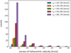 |
Fig. 1 Number of hyperbolic events from the CAMS database with extreme excesses of heliocentric velocities (exceeding the parabolic limit by more than 10 km s−1) for selected intervals of their geocentric velocities υɡ. The x-axis shows the selected intervals of excess of heliocentric velocity (from 10 to 45 km s−1, with bin size 5 km s−1) and the bars illustrate the number of events for corresponding υɡ (as stated in the legend) contained within those intervals. The histograms illustrate two distinct features observed in many databases. One, the presence of hyperbolic events, including those with high heliocentric excess velocities, among meteors with low geocentric velocities. Two, the increase in the number of higher heliocentric excess velocities with increasing geocentric velocities of meteors. |
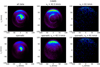 |
Fig. 2 Density plots of the CAMS meteors displayed in relation between the velocity components υx and υy and shown separately for all data (upper panels) and for only sporadic meteors (lower panels). All meteors of these two samples are shown in the left panels, apparent hyperbolic orbits in the middle panels, and a subset of those with hyperbolic heliocentric velocities over 61 km s−1 in the right panels. |
4 Statistical analysis of the CNEOS data
Scientific results derived from data that include uncertainties offer insights into the validity limits of potential conclusions. Since no uncertainties are provided for the parameters in the CNEOS catalog, we have attempted to estimate them to ensure the relevance of the conclusions based on this data. Out of approximately 1000 observed fireballs, we analyzed 291 cases for which the measured parameters allowed estimation of their atmospheric trajectory and calculation of their heliocentric orbit. The measured parameters of six fireballs from this sample resulted in the determination of their orbits as hyperbolic concerning the Sun, including the two suggested interstellar fireball candidates IMC1 and IMC2 (see Table 2).
Parameters of the six nominally hyperbolic CNEOS fireballs.
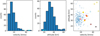 |
Fig. 3 Histograms of velocities (left panel) and altitudes (middle panel) for all CNEOS events. The two interstellar candidates are color coded as filled (IMC1) and empty (IMC2) cyan dots. The right panel shows the altitude–velocity scatter plot, in which six events (including the both interstellar candidates) have significantly deviated from the bulk of the events. The hyperbolic fireballs are marked as red crosses. Events with large deviations in the υy velocity component are shown in orange. The empty square is the CNEOS event 2015-01-07, for which the velocity was overestimated by 30% (Borovička et al. 2017). |
4.1 Velocity distributions and their associated statistical uncertainties
Figure 3 shows histograms of the velocity and altitude, and their mutual relation, and Fig. 4 the same graphs separately for each vector component, as provided in the CNEOS catalog. In all figures, the hyperbolic fireballs are represented by red crosses and the IMC1 and IMC2 are indicated by cyan full and empty dots, respectively.
The overall velocity distribution (left panel of Fig. 3) reveals that most fireballs in CNEOS have (Earth-centered) velocities below 30 km s−1, exhibiting a peak at 17–18 km s−1. There is no significant population visible beyond 40 km s−1. This is to be expected because USG sensors monitor very bright fireballs only, which are likely to be of asteroidal origin therefore impact the Earth on prograde orbits. Other observations from High-Power Large-Aperture (HPLA) radars, based on transverse scatter geometry for the faintest so far recorded radar meteors (mag 16+) indicate a similar peak of the velocity distribution, but exhibit a second peak around 50–60 km s−1 (Schult et al. 2020), corresponding to long-period cometary orbits, that is not present in the CNEOS database. Other radar and optical meteor observations for larger meteoroids also revealed bimodal velocity distributions (Brown et al. 2005; Kornos et al. 2013; Colas et al. 2020; Vida et al. 2021b). Since the velocity distribution in CNEOS is similar to that of the prograde population reported for smaller particle sizes, it implies that the detection probability for potential interstellar meteors should be similar as well, considering that the meteoroids must have similar orbital characteristics (source radiants and velocities).
The velocity distributions carry valuable information about the statistical errors of the observations. In fact, the distributions of υx and υy (see Fig. 4) should look almost identical, as both vectors lie in Earth’s equatorial plane and thus have the same detection probabilities for the velocity spectrum. Such a similarity is only achieved for velocity bin sizes up to 7–8 km s−1, which can thus be regarded as an estimation of the intrinsic statistical uncertainties of CNEOS. The bin size was estimated considering υx and υy measurements as a mean result of all data points used in the analysis of the raw images, and thus according to the central limit theorem, statistics over the entire CNEOS catalog should reflect a Gaussian distribution that looks similar for υx and υy concerning the first two statistical moments (mean and variance).
This becomes even more obvious when looking at the distribution using only a bin width of 2 km s−1 (red bars). These histograms exhibit substructures or peaks at certain velocities in one component, which are missing in the other components. Such features are often the result of discretization errors or observation biases. Unfortunately, these biases could only be quantified from the raw images, which are not available. Furthermore, we verified these bin sizes by applying Scott’s normal reference rule (Scott & Kosar 2015). We also performed a statistical analysis implementing the Freedman–Diaconis rule to estimate the optimal bin size (Freedman & Diaconis 1981), which reduces the influence of statistical outliers by computing the interquartile range of the data. Removing outliers (such as both interstellar fireball candidates) from the analysis, the intrinsic statistical uncertainty is 5–6 km s−1, independent of the applied method. However, even for these large bin sizes, both potential IMCs are still in the tail of the distribution.
Both fireballs are neither the fastest in the catalog (considering the geocentric speed) nor do they show exceptional velocities for the υx and υz velocity components. However, the υy-velocities indicate that both events are in the tail of the υy-distribution (top middle panel of Fig. 4). There are a couple of other CNEOS events that are also found behind a gap in the tail of the velocity distribution (with vy < −35 km s−1 and υy > 20 km s−1) and thus will also be included in the following discussion. Except for the IMC1 and IMC2, only one other event of the orange-labeled fireballs was hyperbolic.
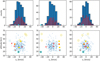 |
Fig. 4 Deviations in the velocity components. Upper panels: histograms of each of the velocity components for all CNEOS events. The red histograms assume a bin width of 2 km s−1. Lower panels: altitude-velocity plots for each of the velocity components. For easier identification of individual events in the histograms, the x-scales for the top and bottom panels are aligned. The symbols are consistent with those in Fig. 3. |
4.2 Extreme deviations in velocity components
In general, meteor measurements show that as velocity component values increase, their contribution to higher total velocities also increases. Thus, any deviation of the velocity components from the majority of events in the dataset results in a high meteor velocity relative to the Earth, and consequently, a high velocity of the meteoroid relative to the Sun, as illustrated by the CAMS meteors in Fig. 2. At the same time, we know that, as the velocity of the meteor increases, the error in determining this velocity also increases, since the number of data points available for estimating the velocity decreases (Vida et al. 2020). An anomalous deviation in a velocity component might therefore reflect a large uncertainty value of the velocity.
The scatter plot in Fig. 3 shows that, except for one, all CNEOS fireballs with total speeds exceeding 35 km s−1 are caused by observations belonging to the events with an excess velocity in the υy-component. This is remarkable, as statistically one would expect equal participation of these events between vx and υy vector velocities. As seen in Fig. 4 (lower middle panel), all of these events are separated from the bulk distribution in the υy velocity versus altitude plot but reflect no velocity-altitude dependence. The largest excesses in this component, among all 291 fireballs in the catalog, belongs to the interstellar candidate IMC1, υy IMC1 = −43.5 km s−1. To better comprehend the relation between the total velocity and the deviations in the velocity components, we plotted each velocity component against the velocity module for each event in the CNEOS catalog (Fig. 5 upper panels).
There is only one fireball, CNEOS 2015-01-07, with total speed above 35 km s−1 (marked with empty square in all figures) that doesn’t have an excess in the υy velocity component, but it does have excess in the υx component. This is the Romania fireball, which has also been independently detected by ground-based observations. Borovicka et al. (2017) determined that the speed of this fireball, 35.7 km s−1 as reported by the USG (with υxRomania = −35.4 km s−1), was 8 km s−1 higher than the actual speed (almost 30%), and the radiant was off by seven degrees from the real position. Consequently, the fireball’s orbit is, in reality, asteroidal with an aphelion just above 4 au, rather than distinctly cometary with an aphelion at 9.2 au as indicated by the CNEOS parameters (Borovicka et al. 2017).
Among the highest velocities, there is another group of events with large deviations in the υy component (marked with empty yellow circles) that resulted in, although not hyperbolic but spurious heliocentric orbits. Their entry velocities of around 50 km s−1, in combination with their angular elongations from the radiant being around 50° (see also Sect. 6.2), indicate nearly perpendicular encounters, which are extremely rare. They require either an almost 90-degree inclination or a very small perihelion distance (Kresák & Kresáková 1976). Such orbits are typically not present in high-precision observations, but they can be found among meteoroid orbits determined from rough velocity data. Consequently, such biased observations lead to an enhancement of meteoroids with small perihelion distances. The three spurious CNEOS fireballs have perihelion distances of 0.09, 0.01, and 0.19 au, respectively. The recently observed Iberian superbolide, measured to have a high velocity, has also been reported to have a low perihelion distance of 0.12 au (Peña-Asensio et al. 2024a).
Generally, such perihelia are considered far too close to the Sun to be realistic for meteoroids that cause fireballs. When approaching distances of less than 0.10 au from the Sun, larger meteoroids commonly tend to rapidly disintegrate (Kresák & Kresáková 1976). Analyzing meteoroid populations of different sizes, Wiegert et al. (2020) showed that a population of meter-sized bodies is absent among the low perihelion orbits, while a population of millimeter-sized meteoroids is observed well within the 0.07 au limit suggested for super-catastrophic disruption of asteroids by Granvik et al. (2016). The distance at which destruction occurs is greater for smaller asteroids (Granvik et al. 2016) and corresponds to 0.36 au for meter-sized bodies (Wiegert et al. 2020).
The fact that the parameters of almost all fireballs with a deviation in one of the velocity components led to their resulting orbits being spurious suggest that large deviations in velocity components result in biased orbits. Consequently, the fact that all fireballs with resulting velocities larger than 35 km s−1 have a deviation in the υy or υx component raises doubts about their measured velocities. This claim is supported by another example of an originally high velocity measurement that shows an extreme deviation in the υz component, which has proven to be erroneous.
It is visible in Fig. 5 (top right panel), in the lower right corner of the plot, where it deviates from the bulk of other events with a low overall velocity. It belongs to the CNEOS 2018-12-18 event, with the resulting velocity of 13.6 km s−1, as provided in the catalog, which is, however, not compatible with its reported components of 6.3, −3.0, and −31.2 km s−1, respectively. This case pertains to the Bering Sea fireball (discussed by Borovička et al. 2020), originally reported to have a total velocity of 32 km s−1. Brown & Borovička (2023) have noted that the original speed of 32 km s−1 posted on the CNEOS site was later amended to 13.6 km s−1. This suggests that this particular case was originally mis-measured by 18.4 km s−1, with a deviation in the component υz BeringSea = −31.2 km s−1. This component, which caused the large original speed, has not been corrected and is still on the website. If the total velocity were not amended, the event would be among those fireballs with the highest apparent velocities that create a tail in the distributions in Fig. 5, among which were found the two interstellar candidates. This discussion provided an additional insight into the possible uncertainties of the CNEOS velocity measurements.
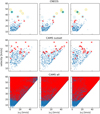 |
Fig. 5 Relation between the total velocity and the absolute value of υx, υy, and υz components for the CNEOS catalog compared with the CAMS data. All hyperbolic events are marked with red crosses, elliptical orbits are shown with blue dots. In the CNEOS data (top row), the symbols are consistent with those in previous figures. For a rough comparison, a subset of 484 sporadic events with prograde orbits (inclination less than 60 degrees) and peak brightness greater than −3 mag was generated from the CAMS database (middle row), approximating the population of CNEOS fireballs. The bottom row displays all CAMS data corresponding to the offset provided by the axis alignment. |
4.3 Hyperbolic velocities
Three of the six CNEOS hyperbolic events, including IMC1 and IMC2, exhibit large deviations in the υy component. The other three hyperbolic fireballs, which fall within the bulk of the υy distribution, are found in or close to the tail of the υx component distribution (Fig. 4). Deviations in this component are not as large as in the υy-component, but nevertheless, two hyperbolic events have the third and eighth largest excesses in υx in the catalog.
The plots in the lower panels of Fig. 4 show that all of them belong to the tail in one of the velocity component distributions, and the plots in the upper panels of Fig. 5 show that all with the excess in υy-component are also on the tail of the total velocity distribution. The other three hyperbolic events have lower entry velocities, with the lowest being 19.1 km s−1. A hyperbolic heliocentric orbit does not require a high velocity relative to the Earth.
The middle and lower row panels of Fig. 5 show the same distributions using the CAMS data to demonstrate a similar behavior of creating artificial hyperbolic meteors. To roughly compare these different datasets, we utilized a subset of the CAMS data that could approximate, at least to some extent, the population of fireballs observed by CNEOS (middle row). Based on the CNEOS catalog information, we filtered all sporadic prograde meteors from the CAMS with inclinations of less than 60 degrees and a brightness of more than −3 mag. The generated subset from the CAMS database comprises 484 orbits, of which 4% are hyperbolic. This subset contains at least ten of meteors with similar characteristics to the two interstellar CNEOS candidates. In the whole CAMS dataset, there are 818 meteors with extremely high heliocentric velocities over 61 km s−1, similar to IMC1. Of course, these particles do not represent a population of interstellar meteoroids (see Sect. 3.3). Panels in the lower row of Fig. 5 show CAMS data corresponding to the offset provided by the axis alignment. In this data file, with common values of uncertainties (~2º in radiant position and ~10% in velocity, Jenniskens et al. 2011), both the overall velocity and the deviation in each of the components reach 100 km s−1. This suggests that the estimated uncertainties are greatly exceeded at high speeds. These plots also illustrate the overlap between the elliptical and hyperbolic populations of meteors that have velocities with respect to Earth spanning the entire interval, down to velocities under 20 km s−1. We would like to emphasize that neither the authors of the CAMS catalog (Gural 2011; Jenniskens et al. 2011, 2016) nor any meteor scientists using these data have ever claimed to discover interstellar particles (Jenniskens, private communication).
To illustrate the fact that all of the putative interstellar fireballs in the CNEOS catalog exhibit a large deviation in one velocity component, which indicates a possible mis-measurement of this component that consequently biases the resulting value of the velocity, we created Fig. 6 showing the distributions of the υx versus υy components, accompanied by histograms using a bin width of 2. The strength of the argument is not only in the magnitude of the excess values of one of the velocity components but also in the fact that all of the nominally hyperbolic fireballs are on the tails of the velocity-components distributions. Those with deviations in the υy component create a gap in the velocity-components distributions (clearly evident in the histograms of Fig. 6). Why interstellar particles should exhibit such a feature is unknown to us.
There is no reason for interstellar particles to exclusively reside in the tails of the distribution of measurements, let alone beyond the gap in the distribution, as they create a phenomenon in the atmosphere like any body entering the atmosphere does. Even meteors created by space debris, which enter the atmosphere at very small angles and low velocities, are not “outliers” in the measurement distributions. Most of them constitute a low-velocity tail of entry speed distribution, since their characteristics are derived with respect to the Earth. But the characteristics of interstellar meteoroids are derived with respect to the Sun, not to the Earth. Their velocities with respect to Earth may cover the entire interval from 12 km s−1 to over 72 km s−1, clearly visible in Fig. 5 (see also Sect. 2.1).
There might be preferable apparent directions of interstellar particles with respect to the Sun connected to a hypothetical source star, and their concentration to the solar apex with the right ascension α = 272º and declination δ = 37º (e.g., Murray et al. 2004). This, however, would be visible only in the case of a larger population of interstellar particles. The radiants of the six CNEOS hyperbolic cases, as determined by Brown & Borovicka (2023) and Peña-Asensio et al. (2024b), do not indicate any common source nor are they aligned with the solar apex. Derived radiants of IMC1 and IMC2 in the equatorial coordinates are: α = 88.5º, δ = 13.3º, and α = 170.2º, δ = 34.3º, respectively (Brown & Borovicka 2023).
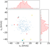 |
Fig. 6 Relation between the velocity components υx and υy. All CNEOS hyperbolic events (red crosses) are on the tail of either the υx or υy distribution. IMC1 and IMC2 are indicated with full and empty cyan colored dots, respectively. The empty square indicates the Romania fireball, the velocity of which was overestimated by 30%. |
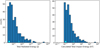 |
Fig. 7 Histograms of radiative energy and impact energy for all CNEOS fireball events. The IMC1 and IMC2 candidates are visualized with full and empty cyan colored dots, respectively. |
4.4 Atmospheric flight physics and aerodynamic constraints
Entering the Earth’s atmosphere at hypersonic speeds leads to several phenomena such as the heating of the object due to atmospheric drag, the formation of a bow shock (Silber et al. 2018), and eventually the vaporization of material of the entering body. The atmospheric flight of meteoroids is modeled using meteor ablation models such as the Chemical Meteor Ablation Model (CABMOD) (Vondrak et al. 2008), the Meteor Ablation Model for Radio-optical Surveys (MARS) (Schult et al. 2015, 2020) or many others. These models assume the conservation of energy and momentum of a meteoroid along the flight path. Thus, the top-of-atmosphere kinetic energy of a meteoroid entering the atmosphere needs to be dissipated along the flight path. In particular, this is the case for all events without kinetic surface impact.
Both interstellar fireball candidates are reported with very large velocities (44.8 km s−1 and 36.5 km s−1) at their termination altitudes of 18 and 23 km. Such deep penetration into the atmosphere requires an efficient cooling mechanism. Usually, meteoroids are cooled down a bit by the phase transition from solid to liquid and finally, the meteoric material vaporizes. Reen-tering objects that are not ablating need to absorb the energy in the material or dissipate the energy in the shock front. Both processes result in ionization and black body emissions and thus in a detectable infrared or visible signature.
The Maribo Fireball is a good example of one for which a combination of sensors observed it along different parts of its trajectory (Schult et al. 2015). The bolide had a top-of-atmosphere velocity of 28.54±0.46 km s−1. This velocity was determined from radar data, just by observing the ionization caused by sputtering (Hill et al. 2004; Rogers et al. 2005). The first detection occurred at an altitude of 116 km and the last and the lowest radar data showed an altitude of 86 km, corresponding to the height of the first visible data recorded by several cameras (Schult et al. 2015, and references therin). The light curve had a length of about 5 seconds. Furthermore, the chemical composition was determined from meteorites found on the ground and was thus used to improve chemical ablation modeling with MAGMA to compute the vaporization pressures for eight metallic oxides (Fegley & Cameron 1987; Schaefer & Fegley 2004; Schult et al. 2015).
The combination of much higher velocities but much shorter light curves (0.54 seconds and 1.4 seconds, corresponding to visible trajectory lengths of 24 and 50 kilometers, assuming the velocities are correct) of both interstellar candidates are not understandable from an energy conservation perspective. The energy equation for a meteoroid is given by
 (2)
(2)
Here, R is the radius of the object (cross-section), v is the velocity, ρa is the atmospheric density, Λ is a heat transfer coefficient, σSB is the Stefan-Boltzmann constant, ϵ is the emissivity, T and Ta are the meteoroid surface and atmospheric temperature, respectively, ρm denotes the meteoroid mass density, C is the heat capacity, L is the heat of fusion, dT/dt-denotes the temperature change and dm/dt describes the mass loss due to vaporization. Although this equation is idealized and assumes a spherical shape of the meteoroid, it illustrates the issue of heating due to atmospheric friction. The source term on the left of the equation is defined by the cross-section of the object, its velocity, and the atmospheric density at the corresponding altitude. The kinetic source energy can be balanced by black-body radiation according to the Stefan-Boltzmann law, heating of the object, and the vaporization/ablation due to the phase transition. The argument presented in Siraj & Loeb (2022b) about the tensile strength is of minor relevance. More importantly, it remains unclear how the meteoroid was able to dissipate the kinetic energy along the flight path without producing a visible light curve at higher altitudes if it were interstellar. Modeling of the Maribo fireball, which entered the Earth’s atmosphere at a much slower velocity of 28.54 km/s started to have a visible signature at approximately 86 km and reached a terminal altitude of 32 km (Schult et al. 2015; Haack et al. 2012). The total length of the light curve was about 4 seconds.
Figure 7 shows histograms of the radiative energy and the impact energy. All of the filtered events fit well into the bulk of the CNEOS observations. Both interstellar candidates (full and empty cyan dots) did not show an exceptionally high radiative energy (3.1 × 10¹⁰ J and 40.0 × 10¹⁰ J) nor did they reflect a high impact energy (0.11 kt and 1.0 kt), although they are among the meteors with the top five highest velocities out of the 291 fireballs in the database (44.8 km s−1 and 36.5 km s−1). Conversely, their radiative energies and low altitudes for both IMCs are in agreement with the bulk of typical JFC comets but are not consistent with their high velocities.
This brief inspection aligns with the findings of an analysis conducted by Brown & Borovička (2023), who modeled the event’s light curve. Their model indicated a potential match, assuming a stony impactor, only when the speed of the event was 20 km s−1 lower than reported. An iron impactor, which would match the reported high speed, would result in significant mass loss and much higher brightness, which was not observed. The authors concluded that it is impossible to fit the observed light curve with the reported speed and altitude.
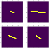 |
Fig. 8 Four real double station meteors as observed by the virtual camera placed at an altitude of 35 800 km. Although the central part consisting of four pixels is the same, the overall shape of the meteors appears different. What is more important, the meteors originated from different radiants. |
5 Simulation of uncertainties due to image resolution
Although CNEOS does not provide raw images for the events, the catalog mentions that after 2019, data from the GLM on the recent generation of GOES satellites is also used to detect bolides. These are listed in a separate database. This information provides a first reference to assess the possible accuracy of the trajectory information. Fortunately this instrument is well documented in the literature (Goodman et al. 2013) and was used as a benchmark for the observations. The GLM catalog of bolides includes (to date) about 5000 detections, which is significantly more than CNEOS, and thus, it is conclusive that GLM provides a lower threshold for the resolution and capabilities to obtain trajectory information. The data analysis pipeline and some initial results from GLM are presented by Jenniskens et al. (2018) and Smith et al. (2021). These examples indicate issues of discretization effects due to the pixel size and pixel noise on the trajectory compared to ground-based observations. There are also other U.S. sensors contributing to CNEOS flying in near-Earth orbits that could achieve a much higher spatial and temporal resolution suitable to obtain precise trajectory information. However, information about the resolution, the spectral observation band, and other important data are not disclosed and thus could not be considered to confirm the reliability of the events.
Both interstellar fireball candidates were also observed during the operation period of the GOES-N series, but these are less well documented. The spatial resolution for the different infrared and visible channels ranges from pixel sizes between 4 × 4 km to 8 × 8 km. Only during daytime there is a visible channel that can reach a 1 × 1 km spatial resolution, and both IMCs were observed during the night. Since the pixel resolution of GOES is about 8 kilometers (GOES-N data book4), in one case most likely only 2–3 pixels were available for the trajectory determination and in the other case 3–4 pixels. Thus, for both interstellar fireball candidates, the trajectory is considered to be prone to large projection errors of up to 45° and more, which translates to errors in the velocity of about 30–40% depending on the velocity component. Even if we assume the 4-kilometer resolution as a reference value, we obtain velocity errors of 20–30% for some vector components. However, without the raw images for both events and information about the observing sensor, it is more reasonable to assume the larger value of a spatial resolution of 8 × 8 km pixel resolution, which refers to a nominal value and might not be achieved at all locations over the full image disc (see GLM for more details).
We created a simulation that replicates the probable observational conditions of the CNEOS fireballs as if they were captured by GLM, and it allowed us to estimate the accuracy of the mete-oroid trajectories as detected from the orbit. The simulation is based on real meteor data obtained during the double-station video experiment (Koten et al. 2020). Known atmospheric trajectories of about one hundred meteors were used. In the simulation, the camera was virtually placed at an altitude of 35 800 km above the surface and these meteors were observed with the resolution of 4 and 8 km px−1, respectively. We omit the brightness of the meteors and focus only on the shape of their images on the virtual detector. As the meteors recorded by GLM are usually detected only on 2 to 4 pixels of the detector, we also concentrate on the central (i.e., the brightest) of our simulated meteors, which contains only 4 pixels. Four meteors with the same central shape consisting of 4 pixels oriented horizontally are shown in Fig. 8. In the second simulation, the central four pixels were oriented vertically.
Although the central parts of meteors look similar on the detector, the azimuths and zenith distances of their radiants vary in both simulations as Fig. 9 shows. In first simulation the radiants of 25 meteors vary between 60° and 90° in azimuth and between 25° and 45° in zenith distance. In addition, there are two outliers with even larger differences in azimuth. In the second simulation, it is between 150° and 180° in azimuth and between 10° and 60° in zenith distance among 14 meteors. With fewer pixels, the scatter of radiants may be even higher.
We note that we considered the best-case scenario, with meteors observed at nadir. At the edge of the field of view, the resolution is lower, which could result in the same appearance of meteors with even more different radiants. Moreover, higher spatial resolution results in lower signal sensitivity. This means that a smaller number of pixels detect the meteor. Again, it could cause even wider spread of possible radiant directions. This illustrates how imprecise the radiant determination from the orbit may be, and supports the findings by Brown & Borovicka (2023), who determined that the median error in radiant is slightly over 30° for a significant majority of the 17 CNEOS events simultaneously obtained by ground-based detections. From ground-based observation, the radiant of the meteors reaches sub-degree precision.
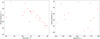 |
Fig. 9 Dispersion of the radiants. The radiants of the video meteors that display identical patterns on a simulated geostationary detector show a wide scatter, ±15°, which indicates a very low accuracy for the radiant determination. The left image displays meteors with a central part consisting of four pixels oriented horizontally (see Fig. 8) and observed at a resolution of 8 km px−1. The right image shows meteors with four central pixels oriented vertically and observed at a resolution of 4 km px−1. |
6 Sensitivity analysis of the hyperbolic fireballs
6.1 Orbital data
Starting from the data provided in the CNEOS catalog (date and time UT, geographical coordinates, and the x/y/z ECEF components of the pre-impact speed vector), we computed the pre-atmospheric heliocentric orbit of each event. To do so, we adopted the classical orbit computation method by Ceplecha (1987).
Two important comments should be taken into consideration for this analysis. First, we assume that the speed module reported in the CNEOS catalog can be interpreted as the pre-atmospheric value of the meteoroid, which is a measure of the speed at the top of the atmosphere before deceleration due to atmospheric drag. We cannot verify this assumption because no other information is provided by the catalog, and it is not clear if the USG sensors are able to measure the deceleration profile of the event and therefore correct for the atmospheric drag. This correction is fundamental when computing the orbital parameters of the meteoroid from the observed speed vector, and it has been demonstrated by various authors that a significant bias originates if not accounting for this effect (see for example Jansen-Sturgeon et al. 2019). Nevertheless, neglecting the atmospheric drag correction will result in an underestimation of the actual pre-atmospheric speed value. Thus, our computation will not generate an apparently open orbit from a closed one. Secondly, the classical orbit computation method by Ceplecha (1987) does not account for the gravitational interaction of other major bodies in the Solar System except for the Sun and the Earth. However, Siraj & Loeb (2022a) used a numerical N-body integrator (Rein & Liu 2012) and mentioned that there are no substantial gravitational interactions between the IMC1 mete-oroid and any planet other than Earth. Therefore, we do not expect these corrections to be significant, at least for the case of IMC1.
To verify and cross-check the results of our implementation, we compared the output of our processing with the orbital elements given by Brown et al. (2016) for 43 fireballs of the same catalog. The observed speed and radiant are used to estimate the geocentric quantities (again, speed and radiant), by correcting for the effect of the Earth’s gravitation attraction, which are finally related to the components of the heliocentric speed vector and provide the values of the orbital elements under the assumption (Dubyago 1961). The relative residuals of the orbital elements, computed for the CNEOS catalog data, outlined a standard deviation of 0.7% for the values of the semimajor axis (a), 2.9% for the orbital eccentricity (e) and 2.4% for the inclination with respect to the ecliptic plane (i), which are within the precision level given by the last significant figure of the speed components reported in the CNEOS catalog.
The orbital elements we calculated for the six nominally hyperbolic fireballs (see Table 2) are in great agreement with the values calculated by Brown & Borovicka (2023) for the same sample but they are slightly less consistent with the values derived by Peña-Asensio et al. (2024b), mostly in the semimajor axes. In Table 2, we also list the altitudes and velocities as provided in the catalog to demonstrate that all of them exhibit an excess in at least one of the velocity components (see Sect. 4). The deviations in one of the velocity components likely resulted in an overestimation of the final velocity and thus have caused the shift in the semimajor axis causing hyperbolas.
Except for three fireballs (none of them hyperbolic), the heliocentric orbits of the entire CNEOS sample are prograde, with a maximum inclination of 54 degrees. The low inclinations of the six nominally hyperbolic events (see Table 2) suggests ecliptic meteoroids. In the case of interstellar particles arriving into the Solar System, a random distribution of their inclinations would be expected. As derived by Peña-Asensio et al. (2024b), the likelihood of detecting six interstellar objects with orbital inclinations smaller than 25° is approximately 0.00007%.
Retrograde orbits are often considered to be one of the indicators supporting interstellar origin. For instance, in the Advanced Meteor Orbit Radar (AMOR, Baggaley et al. 1993b,a) survey, the contribution of retrograde orbits in the closed orbit population was only 5%, while among open orbits it was 41% (Baggaley 1999). However, this fraction was found to be substantially over-represented due to ionization efficiency, which increases with speed (Galligan & Baggaley 2002). The bias of measurement errors increasing toward higher velocities leads to a higher proportion of open orbits in all databases. Consequently, it causes an increase in the proportion of retrograde orbits among the apparent hyperbolic population. Therefore, one must be careful when evaluating retrograde orbits in this context; it is necessary to analyze the entire database.
The only three retrograde orbits in the CNEOS catalog belong to the three fireballs having extremely large deviations in the vy velocity component (depicted as empty orange dots in all figures), causing, in this case, spurious low-perihelion orbits (see Sect. 4).
6.2 Meteor measurement errors versus meteoroid orbit
Fig. 10 shows the computed orbital data of the 291 CNEOS fireballs plotted in a diagram that illustrates the required measurement accuracy for discrimination of various kinds of orbits, as proposed by Kresák & Kresáková (1976) (hereafter referred to as Kresaks’ diagram). Due to the strong correlation between the geocentric velocity (υ𝑔) and the angular elongation (ϵA) of the radiant’s apparent position from the Earth apex, this discrimination is given by the resolution within the specific zone in the diagram. The relation between the two quantities is given by the equation for the heliocentric velocity (υh) of a particle moving in the Sun’s gravitational field:
 (3)
(3)
where υ0 is the mean heliocentric velocity of the Earth. The use of Kresaks’ diagram is particularly important when investigating hyperbolic meteors, as suggested by Hajduková et al. (2019), as it enables us to simultaneously observe the potential uncertainties in both meteor parameters (speed and radiant position) and the resulting meteoroid orbit, thereby understanding the impact of errors on the resulting orbit. In other words, it allowed us to estimate the magnitude of errors (either in each of the two parameters separately or simultaneously in both) that might have caused the shift of the elliptical orbits to apparent hyperbolas.
The red curve in the diagram represents the parabolic orbit, and the six meteors beyond this curve were determined as hyperbolic (red crosses). As introduced in the previous section, the two cyan (full and empty) dots highlights the IMC1 and IMC2 events, and the remaining six events with the an excess in the υy-component are plotted in orange.
The meteor with the largest hyperbolic excess in Fig. 10 is IMC1. Its reported parameters in the CNEOS yield a heliocentric velocity of about 61 km s−1 (see 2 Siraj & Loeb 2022a; Brown & Borovička 2023). Such an extremely high value of the heliocentric velocity exceeding the parabolic limit by approximately 19 km s−1 would require an arrival speed at the edge of the Solar System of about 44 km s−1. This is not in line with the expectations for interstellar meteoroids, based on the nearby stellar velocity distribution (Socas-Navarro 2023; Mamajek 2017, see also Sect. 2.1). For comparison, the arrival speed of ‘Oumua-mua was determined to be 26 km s−1 (Meech et al. 2017), which is very similar to the local standard of rest, and consistent with expectations for interstellar objects (Cabot & Laughlin 2022). The entry speed of Borisov is slightly higher at 32 km s−1 (Guzik et al. 2020).
Socas-Navarro (2023) attempted to explain the extremely high excess velocity of the IMC1 by its gravitational encounter with a massive body corresponding to the hypothetical Planet Nine. However, this hypothesis would not resolve all of the IMC1’s anomalies (extremely low altitude for the high velocity) and, as was already noted by the author, it relies on the unconfirmed existence of Planet Nine and the original hyperbolic orbit of IMC1.
Figure 10 offers a different approach to explain the high velocity by estimating the magnitude of measurement errors required for the resulting orbit to be hyperbolic: When solely considering the velocity error, the shift (along the x-axis) of the orbits for the cases IMC1 and IMC2 beyond the parabolic threshold could potentially be attributed to the uncertainty in velocity of 20 km s−1 and 10 km s−1, respectively. When solely accounting for errors in the radiant position, a level of an uncertainty of 60° and 30°, respectively, could explain the orbital shift (along the y-axis) toward hyperbolic. In the case of such large error values, an error in only one parameter would be sufficient to shift the observed events into the region of bound orbits; however, a combination of errors in both parameters would still suffice, even if they were of smaller magnitudes. The other hyperbolic events require a change of only 1–5 km s−1 in velocity measurements and 2–25° in radiant position to cause this shift.
There are several cases reported in the literature where large discrepancies between CNEOS data and ground-based observations were found (e.g., Jenniskens et al. 2018; Drolshagen et al. 2020; Borovička et al. 2017, 2020, and others). For example, Devillepoix et al. (2019) - when comparing the parameters of several particular events from USG data with an independent ground-based observation of the Desert Fireball Network – discovered that the reported velocities from USG could be incorrect by up to 28%, which induces a factor-of-2 error in inferred material strength, and the re-calculated radiants could be off by up to 90°. The authors literally concluded that USG sensor data are insufficiently reliable for orbit determination, essentially disqualifying the use of the database for interstellar meteor searches.
An instrumentally documented meteorite fall in Turkey that occurred on September 2, 2015, differ by more than 90° in azimuth and by 25° in elevation (Unsalan et al. 2019) from the CNEOS database values. Another example was the British Columbia fireball observed on September 5, 2017. Jenniskens et al. (2018) reported differences by ~77° in azimuth and by ~23° in elevation. These discrepancies are in perfect agreement with the expectations from our simulations described in Sect. 5.
And there is also the case of the Bering Sea fireball (see Sect. 4.2). Although it was not observed by ground-based cameras, the originally reported velocity of 32 km s−1 was changed to 13.6 km s−1 by the providers of the CNEOS catalog, indicating that its velocity was overestimated by 18.4 km s−1.
Such cases seem to be the most extreme, but they are not unique, as shown in a comprehensive list of CNEOS events compared to ground-based stations provided by Brown & Borovička (2023). It is worth noticing that in this list the two events with the largest discrepancy in the pre-impact speeds are the fastest ones (Romania and Saricicek’s bolides). In these two cases, the speed was indeed overestimated by 8 and 7 km s−1, respectively. It reflects the trend known from ground-based observations that measuring higher speeds results in higher uncertainties, which was confirmed for CNEOS observations by Brown & Borovička (2023), who stated that the highest speed USG fireballs exhibit the largest difference compared to ground-based estimates. Using a comparison of 17 cases, Brown & Borovička (2023), estimated that a USG speed measurement of 45 km s−1 could be expected to be 10–15 km s−1 above the true speed, with a radiant error of approximately 30°.
It should be mentioned that there is another new case of simultaneously observed fireball by ground based observations and by the USG (CNEOS 2024-05-18), exhibiting a high speed (40.4 km s−1)5 but showing good agreement. This fireball as recorded by the Spanish Fireball and Meteorite Network (SPMN, Trigo-Rodríguez et al. 2004) shows a deviation in speed, in comparison to CNEOS, of only 0.1 km s−1 (published as the Iberian superbolide, Peña-Asensio et al. 2024a). This is in agreement with the fireball’s observation by the European AllSky7 fireball network (EFN, Spurný et al. 2017; Hankey et al. 2020) and evaluated by Shrbený et al. (private communication). This case, however, cannot be considered a representative example of the CNEOS capabilities because it was a very long fireball (14 seconds compared to 0.54 seconds and 1.4 seconds for IMC1 and IMC2, respectively) with a flat trajectory, which is a favorable configuration for CNEOS (Shrbený et al., private communication).
Siraj & Loeb (2022a) have noted that, for the IMC1, the observed speed would have to be off by 20 km s−1 or a radiant off by more than 60° to obtain a bound orbit of this meteoroid, considering the error in only one parameter. In reality, however, both parameters are measured with a certain degree of error and both parameters affect the determination of the orbit. This implies that smaller errors in both parameters than the values suggested above are sufficient to shift this fireball below the red line representing the parabolic boundary in Fig. 10.
Unfortunately, there is no information given about the measurement errors on the ECEF components, nor is this information provided in the CNEOS catalog. To validate their result, the authors refer to an official letter released by the U.S. Department of Defense (Siraj & Loeb 2019, 2022a), which again does not provide a quantification of these uncertainties. Also a 99.999% confidence for the interstellar nature of IMC1 was reported in Siraj & Loeb (2019) but it is not clear how it was deduced.
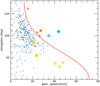 |
Fig. 10 Kresaks’ diagram showing the influence of meteor measurement errors on the resulting meteoroid orbit (based on Kresák & Kresáková 1976; Hajduková et al. 2019). The angular elongation of the apparent radiant from the apex ϵA is plotted against the geocentric velocity υ𝑔 for all 291 CNEOS fireballs. The red curve represents the parabolic limit, beyond which the six hyperbolic CNEOS fireballs (marked with red crosses) are located. The IMC1 and IMC2 fireballs are indicated as full and empty cyan colored dots. The orange dots represent the other υy outliers, three of which (the empty dots around the 45 km s−1 and 40° ) correspond to extremely rare perpendicular encounters. From the resolution of the diagram, one can estimate the uncertainties in speeds and radiant positions that could create the hyper-bolicity of the event’s orbit. |
6.3 On the probability of an interstellar meteor in the data
We wish to test the conclusion of Siraj & Loeb (2022a,b) that IMC1 is extrasolar as well as the conclusion that any of the fireballs in the CNEOS catalog are interstellar. We first use a crude example to illustrate the point that although IMC1 appears to have been interstellar in origin, it would be inevitable in a sample of 1000 meteors, all solar in origin, that at least one would appear to be as anomalous as IMC1.
A crude way to assess the probabilities is to consider the radiant of IMC1 to have been measured precisely, but allow for the fact that the velocity was measured imprecisely, with a 1σ uncertainty6 of about 8 km s−1. Given its geocentric velocity of ≈ 43.8 km s−1, IMC1 would appear interstellar; only if the geocentric velocity were <21.5 km s−1 would it be in an orbit bound to the Sun (as evident from Fig. 10 at the geocentric radiant elongation of IMC1). In this case, a mismeasurement of >22.3 km s−1, yielding a velocity >43.8 km s−1, would be a 2.8 σ result, with one-sided probability 0.26%. If IMC1 were chosen at random and found to have that velocity, it would be 99.74% certain to be interstellar.
IMC1 was not chosen at random, though; indeed, it is the object in the CNEOS most likely to be interstellar. The more appropriate question is: What is the probability that at least one meteor in a catalog of N ~ 103 Sun-bound meteors, would be so mismeasured as to seem as clearly interstellar as IMC1? To estimate this, we assume that any single meteor has a geocentric velocity of 21.5 km s−1, roughly 22.3 km s−1, or 2.8 σ, below the threshold of 43.8 km s−1. As discussed above, any one meteor then has a probability p ≈ 0.26% of being as “clearly” interstellar as IMC1, and the vast majority of Sun-bound meteors will appear Sun-bound, though not all. The probability that at least one object in a catalog of N meteors will appear interstellar is then 1 − (1 − p)N, which for N = 1000 is ≈93%. If we acknowledge that the CNEOS catalog actually provides a velocity estimation for 291 events only, this probability is approximately 53%. Therefore, it is quite probable that such a large catalog, containing only Sun-bound meteors, would contain at least one that appears highly unlikely to be Sun-bound.
To further test the conclusion of Siraj & Loeb (2022a,b), we implemented a simple simulation that assigns a fixed uncertainty σv on the ECEF components (vx, vy,vz) of the speed vector. The value of σv is varied over a reasonable range, from 0.1 to 10 km s−1, corresponding to the uncertainty values in the velocity reported in the literature for various ground-based observation programs. For each event in the database, we then evaluate if the 3σ (99.9%, one-sided) confidence region on the diagram of Fig. 10 crosses on the left of the parabolic limit, becoming compatible with a closed orbit. This is compatible with checking when the resulting confidence interval of the heliocentric speed intersects the parabolic limit vp = 42.1 km s−1 (varying from 41.8 to 42.5 km s−1 along the Earth’s orbit). In this analysis, we will refer to Gaussian symmetric errors as also specified by Siraj & Loeb (2022a), even if this approach provides a lower limit of the estimated errors, because we can expect the velocities of the CNEOS fireballs to be systematically overestimated rather than underestimated, at least for higher speeds (Brown & Borovička 2023).
In fact, one may argue that such discrepancies are to be attributed to systematic deviations rather than random ones, for example, due to the limited resolution of the detector, as for example evident from Fig. 9. However, we are adopting in this analysis the approach of randomization of systematic errors (Wöger 1983; Willink 2013). As a matter of fact, one would not expect the same bias affecting the measurement of the impact speed and radiant direction across the whole CNEOS database, for which the detection of each event over the whole globe is characterized by a different geometry of observation and experimental conditions. Therefore, the final uncertainty on each entry of the CNEOS catalog can be thought of as one value enclosing both terms, which nonetheless remain unknown since they are not directly provided in the catalog.
Figure 11 shows the results of this computation. The left panel plots the number of meteors in the CNEOS catalog that could be confidently identified as hyperbolic, for various assumptions about the absolute value of velocity uncertainty σv. The right panel reports the same result but where σv is varied according to its relative value with respect to each velocity component, from 1% to 50%. Therefore, the inspection of Fig. 11 allows one to understand how the CNEOS hyperbolic subset changes as a function of the indeterminacy of the speed vector components. In particular, the figure shows which is the maximum value of σv, in the case of each of these events, for which the interstellar origin of the estimated orbit would be confirmed beyond the effect of measurement errors. On the other hand, uncertainties above this value would point toward a Solar System origin for these CNEOS candidates, suggesting that the hyperbolic nature of the orbit can be totally explained by measurement errors. In this regard, IMC1 and IMC2 (depicted in cyan) are the events that require the larger values of σv, among the 6 CNEOS hyperbolic events. Both could be confidently identified as hyperbolic, at the >3σ level, for uncertainties up to 1.5 km s−1, or ~7% relative error. However, this is no longer true if σv > 6.2 km s−1, or for a >17% relative error. For IMC1, this corresponds to a standard 1 σ uncertainty on the geocentric speed module of 6.4 km s−1 (15%) and 8° (7%) for the radiant elongation. For IMC2, these values are smaller and correspond to 2.6 km s−1 (8%) and 4° (4%) only. We note that our estimation of σv represents the most optimistic scenario for both events, when considering a 3σ filtering. A 99.999% confidence for the interstellar nature of IMC1 (as reported by Siraj & Loeb 2019) would correspond to just over 4σ in terms of confidence intervals, therefore decreasing the magnitude of uncertainties estimated here according to a 3σ filtering.
Therefore, measurement uncertainties of this magnitude for the CNEOS speed values would explain (at the selected confidence level) IMC1 and IMC2 to be hyperbolic only due to measurement errors and not of an actual interstellar origin. Such values have to be compared with the estimation of the precision and accuracy of CNEOS speed data discussed in the previous sections. The statistical analysis of the distributions of the CNEOS speed components (Sect. 4.1) suggests an intrinsically statistical uncertainty of 5–6 km s−1 that is very close to the minimum value of σv estimated for the case of IMC1 and more than double of the value in the case of IMC2. In a similar way, the simulations of uncertainties due to the image resolution (Sect. 5) suggest that the radiant position may be off from the real value by several tens of degrees (Fig. 9), while we demonstrated that an uncertainty of 8° for IMC1 and 4° for IMC2 is enough to disprove an interstellar origin of these objects at a 99.9% confidence level.
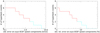 |
Fig. 11 Number of apparent hyperbolic events in the CNEOS catalog as a function of the standard uncertainty σv on each of the ECEF components of the pre-impact speed vector when using a 3σ criterion to check if the confidence region on the Kresak’s diagram crosses the left of the parabolic limit (Fig. 10). The left panel plots the result of this analysis when varying the absolute value of σv from 0.1 to 10 km s−1, whereas in the right panel we varied its relative value with respect to each component from 1% to 50%. The IMC1 and IMC2 candidates (cyan) have been filtered out for σv = 6 km s−1, or a 17% relative uncertainty. |
7 Challenges of recovering interstellar meteorites
If an interstellar meteor were confirmed, it would be of great scientific interest to recover material from it. Here, we provide estimations regarding the feasibility of recovering the IMC1 fragments. Material collection from this fireball as a means of testing the interstellar hypothesis was proposed Siraj et al. (2022), and an expedition to do so has been carried out7.
It is not impossible that interstellar meteoroids could hit the Earth, and it is not impossible that material from such an object could survive entry and be collected. However, it is very unlikely that any material could be collected from the IMC1 fireball in particular, and the inherent challenges highlight the difficulties of recovery of material from any interstellar meteoroid.
First, the high entry speeds likely lead to the near-complete vaporization of the object almost regardless of composition. The IMC1 bolide, in particular, is reported to have traveled at 45 km s−1, at which speed ablation is nearly total.
Meteoroids are ablated and lose considerable mass during entry. The mass loss depends on a complicated balance of the heating (by contact with compressed, heated gas, by frictional flow, and by absorption of radiation from the surrounding gas) and cooling (by conduction of heat into the meteoroid interior), as illustrated by Eq. (2). Many of the relevant factors are absorbed into the ablation parameter σ = Λ/2QCD, where Λ is the heat transfer coefficient, Q is the specific energy of ablation, and CD is the drag coefficient (Popova et al. 2019). Simultaneous integration of the energy and mass loss equations yields the solution for the final mass of the meteoroid:
 (4)
(4)
where Mi is the initial mass when the meteoroid had velocity Vi, and Vf (≈ a few kilometers per second) is the velocity at which ablation ceases (Popova et al. 2019). Based on the optical energy of 3.1 × 10¹⁰ J, a standard luminous efficiency τ ≈ 6.9% (Brown et al. 2002), and a speed of 45 km s−1 when the meteoroid disintegrated, the initial mass of the 2014-01-08 bolide is estimated as Mi ~ 450 kg. Modeling of some specific rocky bolides suggests σ could be as low as 0.004 km−2 s2 (Ceplecha & Revelle 2005), for which Mf might be as high as 8 kg; but the average ablation parameter inferred for rocky meteoroids is σ ≈ 0.014 km−2 s2 (Revelle & Ceplecha 2001), for which Mf = 0.3 g.
This ablation parameter pertains to rocky bodies, but if the IMC1 was moving at 45 km s−1, it was probably iron to survive to 18 km altitude. The ram pressure at which it broke up was approximately 240 MPa (Siraj & Loeb 2022b), comparable to the compressive strength of iron meteorites, but much greater than the typical strength of rocky bodies, 1–5 MPa (Pohl & Britt 2020). It is worth mentioning that Siraj & Loeb (2022b) misquote Pohl & Britt (2020) when they say the strength of iron meteorites is only 50 MPa. Iron vaporizes more easily than rock owing to the much higher heat transfer coefficients of metallic compositions, and the ablation parameter for iron meteorites is more typically σ ≈ 0.07 km−2 s2 (Revelle & Ceplecha 1994). Therefore, Mf is vanishingly small.
In unpublished work by Tillinghast-Raby et al. (2022), it is suggested that a large fraction (>10%) of the bolide would survive entry. This is based on the incorrect assumption that upon disintegration, the bolide would “explode” at 41 km s−1 in all directions, canceling the forward velocity of 45 km s−1 for some of the material. First of all, meteoroids do not explode per se. An explosion involves an exothermic chemical reaction. A meteor light curve spikes because the meteoroids disrupt in many fragments, thus suddenly increasing the total surface area and subsequent ablation rate. Second, meteoroid fragments tend to disperse at only tens of meters per second in the transverse direction of motion, with the main velocity being practically unchanged, as shown by both theoretical and observational works (Passey & Melosh 1980; Stokan & Campbell-Brown 2014).
A second challenge is that this small mass is spread out over a large area, yielding low concentrations of ablated particles. Meteorite strewn fields are typically 4 km wide and at least as long, suggesting a minimum area > 10 km2 (Moilanen et al. 2021). For IMC1, ablated particles additionally would have been subject to the ~1 m s−1 Equatorial UnderCurrent as they sank to the seafloor (Azminuddin et al. 2022). Iron particles of various masses (e.g., 1 g to 1 mg) would take varying times to sink by Stokes flow (20 seconds to 30 minutes), and would be carried varying distances eastward (0 to 2 km), increasing the strewn field area and lowering the concentration well below ~30 mg km−2. Assuming ablated particles are 0.025 mg each, their concentration would be <103 km−2.
Third, in addition to the challenge of finding these particles, is the challenge of distinguishing them from the large background of other spherules on the seafloor, which may be Solar System-derived micrometeorites, microtektites, or spherules of a terrestrial volcanic or industrial origin. Millard & Finkelman (1970) were able to recover spherules from the seafloor using a magnetic sledge, recovering 1200 micrometeorites totaling 30 mg from 750 kg of Pacific red clay. Brownlee et al. (1979) used a similar device to sift through ~107 kg per day. Siraj et al. (2022) proposed to process 6 × 10⁷ kg over 0.4 km2, which is reasonable. However, while they might be expected to recover perhaps hundreds of spherules (totalling 12 mg) from the IMC1 fireball, they would also collect 2.4 × 10⁶ mg of Solar System micrometeorites. That is, fewer than one out of every 200000 collected spherules could be from the IMC1, if any survived at all.
A fourth challenge is locating the strewn field in the first place. Formal uncertainties in the fireball location are not quoted in the CNEOS database, but since the latitude and longitude are stated to one decimal place the uncertainties cannot be less than ±0.1° in latitude and longitude, that is, ±11 km. Siraj & Loeb (2023) have claimed to fix the location of the fireball using a single seismometer. However, this procedure is much more imprecise than they realize, and in any event the only signal they used was one of a passing truck (Fernando et al. 2024). An additional complication is that the material would have moved along the trajectory (to the east) an uncertain distance from the fireball location before impacting the ocean. Considerations of the atmospheric winds produce considerable variations of several kilometres in the estimated location of the strewn field relative to a calm atmosphere (Andreic 2012), adding to uncertainties in the pre-breakup trajectory of the bolide. Last but not least, water currents should be taken into account to estimate the location of at which any spherules might have come to rest at the bottom of the ocean. Siraj & Loeb (2023) do not acknowledge this, and indeed their figures erroneously show the bolide moving to the west.
It is extremely unlikely any material can be collected and confidently assigned to the IMC1 bolide. The location of the fireball, and of the strewn field, is uncertain by at least ±10 km. At the reported speeds, the object would have almost completely vaporized; the concentration over the strewn field would have been <10 mg km−2, perhaps five orders of magnitude lower than the background concentration of Solar System micrometeorites. Highly uncertain contributions from terrestrial sources would further dilute this already very low fraction. These challenges would apply to almost any interstellar meteor, and unusual circumstances would be required for interstellar material to be identified, namely, the bolide would have to approach Earth “from behind” at a low velocity to allow for the survival of fragments greater than kilograms in mass; the velocity and radiant would have to be known precisely enough (< 100 m s−1 uncertainty) to identify it as interstellar; and the entry would have to be tracked on radar in order to fix the location of the strewn field. To be tracked by radar, and to aid recovery, impact on land is practically demanded.
8 Discussion
Examining potential biases and errors is crucial when evaluating the reliability of hyperbolic events as potential candidates for interstellar meteoroids. The rationale is that the sought-after characteristic, the expected hyperbolic excesses of a meteoroid’s heliocentric velocity, closely approximates the uncertainty in velocity determination. Therefore, verifying a genuinely hyperbolic orbit, the sole indicator of an interstellar origin thus far, is extremely challenging (e.g., Hajduková et al. 2020; Hajduková & Kornoš 2020).
The CNEOS catalog includes 954 fireballs (as of May 2023), but velocity and altitude data are available for only 30.5% of all cases, comprising 291 orbits. Out of these, 6 orbits were determined to be hyperbolic. Two of them, IMC1 and IMC2, were suggested as candidates for an interstellar origin (Siraj & Loeb 2022a; Peña-Asensio et al. 2022). They were reported with velocities 44.8 km s−1 and 36.5 km s−1 at their termination altitudes of 18 km and 23 km (see also Table 2). Since the catalog does not report measurement uncertainties, we conducted an assessment of them through independent testing, employing a comprehensive statistical analysis of the data and studying them through modeling.
Here, we summarize our main findings. Together they form a compelling argument that (1) demonstrates that all hyperbolic events in the catalog are most probably the result of measurement errors rather than interstellar origins, (2) undermines the claims for an interstellar origin of IMC1 (Siraj & Loeb 2022a), and (3) refutes the origin of the recovered spherules from the sea floor in IMC1 (Siraj et al. 2022).
8.1 Arguments against the claim that there are six interstellar objects in CNEOS
The determination of the heliocentric orbit of a meteoroid (and its heliocentric velocity) is influenced by meteor measurements of both the velocity and radiant position, the uncertainties of which are therefore crucial for the plausibility of the resulting orbit. Our analyses resulted in the following estimates for both parameters:
The intrinsic statistical uncertainties of the velocities in the catalog were evaluated to 7–8 km s−1 or 5–6 km s−1 but with a more conservative approach (after reducing the influence of statistical outliers; see Sect. 4). According to a 99.9% significance test, we estimated the minimum value of σv = 6.2 km s−1, that is, the standard uncertainty on the ECEF velocity components (measured by USG sensors) beyond which the hyperbolic nature of all CNEOS hyperbolic events can be entirely attributed to measurement errors (see Sect. 6.3). Such a value of σv closely aligns with the estimated intrinsic statistical uncertainties of the speed measurements in the catalog.
The radiants derived from meteor detection from space were found to exhibit significant variations (Sect. 5 and Fig. 9), which indicates a precision of ±15°. Unfortunately, as information on the detector and its spatial resolution or raw data are not available, we can simulate only observations as it would be done using GLM sensor with known properties.
A combination of the estimated uncertainties in velocity and radiant determination would be sufficient to alter the orbits to become hyperbolic for all CNEOS hyperbolic fireballs (Fig. 10 and Sect. 6.2). IMC2 is on the border of the error bars, and IMC1 requires larger values than the above estimates. Given the increase in error magnitude with increasing speed, we can assume that the uncertainties in the parameters of the hyperbolic cases attain larger values than estimated for the whole database.
It is evidenced by significant deviations of the high-velocity events (v > 35 km s−1) in the vy velocity component distributions from the bulk of the other events. The resulting orbits of three of these fireballs are hyperbolic, while three others exhibit another spuriousness. They correspond to apparent perpendicular encounters (Sect. 4 and Fig. 10) causing a bias in perihelion distances, which are, for these three orbits unrealistically small, indicating their incorrect determination. A large deviation in one of the velocity components, vx or vy is present in all six hyperbolic fireballs in the catalog (Sect. 4, and Fig. 6.) There is no reason for interstellar particles to exhibit such an anomaly in the velocity mesurements, as their velocities relative to Earth can span the entire range from 12 km s−1 to over 72 km s−1. Interstellar particles would generate a phenomenon in the atmosphere similar to any object entering it; their unique characteristics should be observable with respect to the Sun rather than Earth. Mismeasurements of this kind are more likely attributable to projection effects (Sect. 4).
Comparison with other meteor datasets demonstrates a similar behavior in the creation of apparent hyperbolic orbits due to meteor measurements, but on a much larger scale. It also shows that the uncertainties estimated by the authors of the catalog are commonly exceeded at high speeds (Sect. 3.3). The hyperbolic samples mainly consist of measurements that exhibit large deviations in the velocity components, which also result in extremely large excess velocities.
Additionally, all of the hyperbolic fireballs from the catalog have low orbital inclinations, suggesting ecliptic particles. The inclinations of heliocentric orbits for interstellar meteoroids are anticipated to be either high or, at the very least, randomly distributed, in the light of the Sun’s galactic environment (Sect. 6).
8.2 Arguments against the claim that IMC1 is interstellar
The probability that at least one object among the 291 fireballs will appear interstellar is approximately 53%, taking into account our velocity uncertainty estimate and considering a zero error in the radiant. For a catalog of 1000 events (corresponding to all of the fireballs in the CNEOS catalog), this probability is approximately 93%. Hence, it is highly probable that a catalog such as CNEOS, containing only Sun-bound meteors, would contain at least one that appears highly unlikely to be Sun-bound (like the IMC1) (Sect. 6.3).
For the case of IMC1, the minimum value of σv = 6.2 km s−1 (see above) corresponds to a standard uncertainty in the geocentric speed module of 6.4 km s−1 (15%) and 8° (7%) for the radiant elongation (Sect. 6.3 and Fig. 11). The error in the radiant elongation falls well within the estimated uncertainty of ± 15° (Sect. 5). The IMC1 exhibits the largest deviation in vy component in the catalog, creating a gap in this velocity component distribution (clearly evident in Fig. 6), which indicates a larger error causing an overestimation of its velocity.
The reported velocity of the IMC1, at 44.8 km s−1, yields a large value of the hyperbolic excess velocity of 61 km s−1, exceeding the parabolic limit by 19 km s−1, which corresponds to an entry speed of this meteoroid into the Solar System of 44 km s−1. Such a value falls within the tail of the velocity distribution of nearby stars and is compatible with only 10% of stars (Sect. 2.1), indicating an unusual source.
A comparison with other datasets demonstrates that such large values of the heliocentric velocities determined from meteor data are not rare (there are tens to hundreds of them in various meteor databases). Since these large hyperbolic meteor populations do not represent populations of interstellar particles, the extreme hyperbolic excess as determined for IMC1 does not seem to imply anything peculiar, but rather reflects a higher error value (Sect. 3.3).
The reported low altitude of IMC1 (18 km) contradicts the reported high velocity. Such a combination of parameters is inconsistent with the principles of energy conservation, as kinetic energy could not have been dissipated without producing visible light at higher altitudes, which was not observed. Therefore, the explanation by the proposed extremely strong interstellar material fails. On the other hand, the low altitude of the IMC1 and its radiative energy are consistent with the bulk of typical Jupiter-family comets and their radiative energies, suggesting a Solar System meteoroid (Sect. 4.4).
The orbital inclination of 9.75° does not correspond to expectations for interstellar particles considering the Sun’s galactic environment, indicating that this meteoroid belongs to an ecliptic population (Sect. 6).
8.3 Arguments against the IMC1 origin of the microspherules recovered by the GALILEO expedition
It is not impossible for an interstellar meteoroid to impact Earth, and for some of its fragments to survive the atmospheric entry. However, the reported IMC1’s speed of 44.8 km s−1 would result in the meteoroid almost total vaporizing in the atmosphere, leaving only insignificant quantities to survive. This small mass is then spread out over a large area, yielding low concentrations of ablated particles (~30 mg km−2), recovery of which is highly unlikely (Sect. 7).
Even if an interstellar origin of a fireball were confirmed, and if any of its fragments were to survive, it would be, in general, a great challenge to confidently assign the recovered material of meteorites found on the seafloor to the observed fireball, considering the presence of numerous micrometeorites from the Solar System, microtektites from Earth, as well as spherules terrestrial volcanic or industrial origins (Sect. 7).
9 Conclusions
Our findings listed above highlight the reasons for the probable overestimation of IMC1’s velocity and provide further arguments questioning the claim of the interstellar origin of this fireball. They complement the results by Brown & Borovička (2023), who demonstrated that the measured light curve of IMC1 cannot be explained by the reported high entry velocity and low altitude.
We conclude that, based on the available data, we find no evidence to validate an interstellar origin of any of the nominally hyperbolic fireballs from the CNEOS catalog, including the two interstellar candidates proposed by Siraj & Loeb (2019, 2022b). We are also aware that the data do not allow us to refute the claim either and that our methods rely on certain assumptions. However, since we have identified several independent reasons that point to substantial uncertainties in the velocity and radiant position of the CNEOS events, we can conclude, applying Occam’s razor, that the simplest explanation is that the discrepancies and peculiarities found in the behavior and parameters of IMC1 and IMC2 are most parsimoniously resolved by assuming that their velocities are overestimated.
Both our approach and results may challenge interstellar meteor surveys in the crucial determination of underlying error distributions for all data – that is, not only for the hyperbolic candidates. Our approach may unveil not only a misdetermina-tion of parameters but also a common tendency to underestimate uncertainties in the databases. This study also demonstrates that the appropriateness of data selection is a crucial factor in ensuring reliable results for targeted analysis and that an analysis of the whole dataset is crucial for the determination of a specific interstellar meteor candidate.
Acknowledgements
The work of M. Hajdukova was supported by the Slovak Grant Agency for Science - VEGA, grant No. 2/0009/22. V.J. Sterken received funding from the European Union’s Horizon 2020 research and innovation programme under grant agreement No. 851544 – ASTRODUST. This research has made use of NASA’s Astrophysics Data System Bibliographic Services.
References
- Almond, M., Davies, J. G., & Lovell, A. C. B. 1951, MNRAS, 111, 585 [CrossRef] [Google Scholar]
- Almond, M., Davies, J. G., & Lovell, A. C. B. 1952, MNRAS, 112, 21 [CrossRef] [Google Scholar]
- Anderson, E., & Francis, C. 2012, Astron. Lett., 38, 331 [Google Scholar]
- Andreic, Z. 2012, in Proc. of the IMC, 30th IMC, Sibiu, Romania, 23 [Google Scholar]
- Azminuddin, F., Jang, C.-J., & Jeon, D. 2022, Front. Mar. Sci., 9, 1 [Google Scholar]
- Baalmann, L. R., Hunziker, S., Strub, P., et al. 2022, in AGU Fall Meeting Abstracts, 2022, SH43B-08 [Google Scholar]
- Baggaley, W. J. 1999, in Meteoroids 1998 Conference, eds. W. J. Baggaley, & V. Porubcan, 265 [Google Scholar]
- Baggaley, W. J. 2000, J. Geophys. Res., 105, 10353 [NASA ADS] [CrossRef] [Google Scholar]
- Baggaley, W. J., Taylor, A. D., & Steel, D. I. 1993a, in Meteoroids and their Parent Bodies, eds. J. Stohl, & I. P. Williams, 53 [Google Scholar]
- Baggaley, W. J., Taylor, A. D., & Steel, D. I. 1993b, in Meteoroids and their Parent Bodies, eds. J. Stohl, & I. P. Williams, 245 [Google Scholar]
- Borovička, J., Spurný, P., Grigore, V. I., & Svoren, J. 2017, PSS, 143, 147 [Google Scholar]
- Borovička, J., Setvák, M., Roesli, H., & Kerkmann, J. K. 2020, A&A, 644, A58 [NASA ADS] [CrossRef] [EDP Sciences] [Google Scholar]
- Borovička, J., Spurný, P., & Shrbený, L. 2022a, A&A, 667, A158 [NASA ADS] [CrossRef] [EDP Sciences] [Google Scholar]
- Borovička, J., Spurný, P., Shrbený, L., et al. 2022b, A&A, 667, A157 [NASA ADS] [CrossRef] [EDP Sciences] [Google Scholar]
- Brown, P. G., & Borovicka, J. 2023, ApJ, 953, 167 [NASA ADS] [CrossRef] [Google Scholar]
- Brown, P., Spalding, R. E., ReVelle, D. O., Tagliaferri, E., & Worden, S. P. 2002, Nature, 420, 294 [Google Scholar]
- Brown, P., Jones, J., Weryk, R. J., & Campbell-Brown, M. D. 2005, The Velocity Distribution of Meteoroids at the Earth as Measured by the Canadian Meteor Orbit Radar (CMOR), eds. R. Hawkes, I. Mann, & P. Brown (Dordrecht: Springer Netherlands), 617 [Google Scholar]
- Brown, P., Wiegert, P., Clark, D., & Tagliaferri, E. 2016, Icarus, 266, 96 [CrossRef] [Google Scholar]
- Brownlee, D. E., Pilachowski, L. B., & Hodge, P. W. 1979, in Lunar and Planetary Science Conf., Lunar and Planetary Science Conference, 157 [Google Scholar]
- Cabot, S. H. C., & Laughlin, G. 2022, PSJ, 3, 172 [NASA ADS] [Google Scholar]
- Ceplecha, Z. 1987, Bull. Astron. Inst. Czech., 38, 222 [NASA ADS] [Google Scholar]
- Ceplecha, Z., & Revelle, D. O. 2005, Meteorit. Planet. Sci., 40, 35 [NASA ADS] [CrossRef] [Google Scholar]
- Colas, F., Zanda, B., Bouley, S., et al. 2020, A&A, 644, A53 [EDP Sciences] [Google Scholar]
- Dehnen, W., & Binney, J. J. 1998, MNRAS, 298, 387 [NASA ADS] [CrossRef] [Google Scholar]
- Devillepoix, H. A. R., Bland, P. A., Sansom, E. K., et al. 2019, MNRAS, 483, 5166 [NASA ADS] [CrossRef] [Google Scholar]
- Devillepoix, H. A. R., Cupák, M., Bland, P. A., et al. 2020, PSS, 191, 105036 [Google Scholar]
- Drolshagen, E., Ott, T., Koschny, D., et al. 2020, PSS, 184, 104869 [Google Scholar]
- Dubyago, A.D. 1961, The Determination of Orbits (New York: The Macmillan Company) [Google Scholar]
- Fegley, B., & Cameron, A. 1987, Earth Planet. Sci. Lett., 82, 207 [CrossRef] [Google Scholar]
- Fernando, B., Mialle, P., Ekström, G., et al. 2024, arXiv e-prints [arXiv:2403.03966] [Google Scholar]
- Fisher, W. J. 1928, Harvard College Obs. Circ., 331, 1 [NASA ADS] [Google Scholar]
- Freedman, D., & Diaconis, P. 1981, Z. Wahrscheinlichkeitstheorie verw Gebiete, 57, 453 [CrossRef] [Google Scholar]
- Froncisz, M., Brown, P., & Weryk, R. J. 2020, PSS, 190, 104980 [Google Scholar]
- Galligan, D. P., & Baggaley, W. J. 2002, in ESA Special Publication, 500, ACM Conf. 2002, ed. B. Warmbein, 225 [NASA ADS] [Google Scholar]
- Goodman, S. J., Blakeslee, R. J., Koshak, W. J., et al. 2013, Atmos. Res., 125, 34 [Google Scholar]
- Granvik, M., Morbidelli, A., Jedicke, R., et al. 2016, Nature, 530, 303 [Google Scholar]
- Gregg, C. R., & Wiegert, P. A. 2023, in ACM Conf. 2023, LPI Contrib. No. 2851, 2164 [Google Scholar]
- Grün, E., Zook, H. A., Baguhl, M., et al. 1993, Nature, 362, 428 [Google Scholar]
- Gural, P. S. 2011, in Proc. of the IMC, 29st IMC, Armagh, Northern Ireland, 2010, 28 [Google Scholar]
- Guzik, P., Drahus, M., Rusek, K., et al. 2020, Nat. Astron., 4, 53 [Google Scholar]
- Haack, H., Grau, T., Bischoff, A., et al. 2012, Meteor. Planet. Sci., 47, 30 [NASA ADS] [CrossRef] [Google Scholar]
- Hajduk, A. 2001, in ESA Special Publication, 495, Meteoroids 2001 Conf., ed. B. Warmbein, 557 [NASA ADS] [Google Scholar]
- Hajduková, M. 1993, in Meteoroids and their Parent Bodies, eds. J. Stohl, & I. P. Williams, 61 [Google Scholar]
- Hajduková, M. 1994, A&A, 288, 330 [Google Scholar]
- Hajduková, M., & Kornoš, L. 2020, PSS, 190, 104965 [Google Scholar]
- Hajduková, M., Sterken, V., & Wiegert, P. 2019, in Meteoroids: Sources of Meteors on Earth and Beyond, eds. G. O. Ryabova, D. J. Asher, & M. J. Campbell-Brown, 235 [Google Scholar]
- Hajduková, M., Sterken, V., Wiegert, P., & Kornoš, L. 2020, PSS, 192, 105060 [Google Scholar]
- Hankey, M., Perlerin, V., & Meisel, D. 2020, Planet. Space Sci., 190, 105005 [CrossRef] [Google Scholar]
- Hawkes, R. L., & Woodworth, S. C. 1997, J. R. Astron. Soc. Can., 91, 68 [NASA ADS] [Google Scholar]
- Hawkes, R. L., Close, T., & Woodwoth, S. 1999, in Meteroids 1998 Conf., eds. W. J. Baggaley, & V. Porubcan, 257 [Google Scholar]
- Heikkinnen, M. 1982, Z. Ermess., 107, 207 [Google Scholar]
- Higuchi, A., & Kokubo, E. 2020, MNRAS, 492, 268 [Google Scholar]
- Hill, K., Rogers, L., & Hawkes, R. 2004, Earth Moon Planets, 95, 403 [NASA ADS] [CrossRef] [Google Scholar]
- Holmberg, J., Nordström, B., & Andersen, J. 2009, A&A, 501, 941 [NASA ADS] [CrossRef] [EDP Sciences] [Google Scholar]
- Hopkins, M. J., Bannister, M. T., & Lintott, C. 2024, arXiv e-prints [arXiv:2402.04904] [Google Scholar]
- Jacchia, L. G., & Whipple, F. L. 1961, Smithsonian Contrib. Astrophys., 4, 97 [CrossRef] [Google Scholar]
- Jansen-Sturgeon, T., Sansom, E. K., & Bland, P. A. 2019, Meteorit. Planet. Sci., 54, 2149 [NASA ADS] [CrossRef] [Google Scholar]
- Jenniskens, P., Gural, P. S., Dynneson, L., et al. 2011, Icarus, 216, 40 [NASA ADS] [CrossRef] [Google Scholar]
- Jenniskens, P., Nénon, Q., Gural, P. S., et al. 2016, Icarus, 266, 384 [NASA ADS] [CrossRef] [Google Scholar]
- Jenniskens, P., Albers, J., Tillier, C. E., et al. 2018, Meteorit. Planet. Sci., 53, 2445 [NASA ADS] [CrossRef] [Google Scholar]
- Jewitt, D. 2024, arXiv e-prints [arXiv:2407.06475] [Google Scholar]
- Jewitt, D., & Seligman, D. Z. 2023, ARA&A, 61, 197 [NASA ADS] [CrossRef] [Google Scholar]
- Kornos, L., Koukal, J., Piffl, R., & Toth, J. 2013, in Proc. of the IMC, 31st IMC, La Palma, Canary Islands, Spain, 2012, eds. M. Gyssens, & P. Roggemans, 21 [Google Scholar]
- Koschny, D., Bettonvil, F., Licandro, J., et al. 2013, Geosci. Instrum. Methods Data Syst., 2, 339 [NASA ADS] [CrossRef] [Google Scholar]
- Koten, P., Spurný, P., Borovicka, J., & Stork, R. 2003, Pub. Astron. Inst. Czech. Ac. Sc., 91, 1 [Google Scholar]
- Koten, P., Borovicka, J., Vojácek, V., et al. 2020, PSS, 184, 104871 [Google Scholar]
- Kresák, L., & Kresáková, M. 1976, Bull. Astron. Inst. Czech., 27, 106 [Google Scholar]
- Krüger, H., Strub, P., Grün, E., & Sterken, V. J. 2015, ApJ, 812, 139 [CrossRef] [Google Scholar]
- Mamajek, E. 2017, RNAAS, 1, 21 [NASA ADS] [Google Scholar]
- Meech, K. J., Weryk, R., Micheli, M., et al. 2017, Nature, 552, 378 [Google Scholar]
- Meisel, D. D., Janches, D., & Mathews, J. D. 2002, ApJ, 567, 323 [NASA ADS] [CrossRef] [Google Scholar]
- Mihalas, D., & Routly, P. M. 1968, Galactic astronomy (W. H. Freeman) [Google Scholar]
- Millard, H. T. J., & Finkelman, R. B. 1970, J. Geophys. Res., 75, 2125 [NASA ADS] [CrossRef] [Google Scholar]
- Moilanen, J., Gritsevich, M., & Lyytinen, E. 2021, MNRAS, 503, 3337 [NASA ADS] [CrossRef] [Google Scholar]
- Moorhead, A. V. 2021, Icarus, 354, 113949 [NASA ADS] [CrossRef] [Google Scholar]
- Morbidelli, A., Batygin, K., Brasser, R., & Raymond, S. N. 2020, MNRAS, 497, L46 [NASA ADS] [CrossRef] [Google Scholar]
- Murray, N., Weingartner, J. C., & Capobianco, C. 2004, ApJ, 600, 804 [NASA ADS] [CrossRef] [Google Scholar]
- Musci, R., Weryk, R. J., Brown, P., Campbell-Brown, M. D., & Wiegert, P. A. 2012, ApJ, 745, 161 [NASA ADS] [CrossRef] [Google Scholar]
- National Imagery and Mapping Agency 2000, Department of Defense World Geodetic System 1984: its definition and relationships with local geodetic systems, Tech. Rep. TR8350.2 (St. Louis, MO, USA: National Imagery and Mapping Agency) [Google Scholar]
- Öpik, E. 1940, Pub. Tartu Astrof. Obs., 30, E1 [Google Scholar]
- Öpik, E. J. 1956, Ir. Astron. J., 4, 49 [Google Scholar]
- Passey, Q. R., & Melosh, H. J. 1980, Icarus, 42, 211 [NASA ADS] [CrossRef] [Google Scholar]
- Peña-Asensio, E., Trigo-Rodríguez, J. M., & Rimola, A. 2022, AJ, 164, 76 [Google Scholar]
- Peña-Asensio, E., Grèbol-Tomàs, P., Trigo-Rodríguez, J. M., Ramírez-Moreta, P., & Kresken, R. 2024a, MNRAS, submitted [arXiv:2405.15024] [Google Scholar]
- Peña-Asensio, E., Visuri, J., Trigo-Rodríguez, J. M., et al. 2024b, Icarus, 408, 115844 [CrossRef] [Google Scholar]
- Pohl, L., & Britt, D. T. 2020, Meteorit. Planet. Sci., 55, 962 [NASA ADS] [CrossRef] [Google Scholar]
- Popova, O., Borovicka, J., & Campbell-Brown, M. D. 2019, in Meteoroids: Sources of Meteors on Earth and Beyond, eds. G. O. Ryabova, D. J. Asher, & M. J. Campbell-Brown, 9 [Google Scholar]
- Rein, H., & Liu, S. F. 2012, A&A, 537, A128 [NASA ADS] [CrossRef] [EDP Sciences] [Google Scholar]
- Revelle, D. O., & Ceplecha, Z. 1994, A&A, 292, 330 [NASA ADS] [Google Scholar]
- Revelle, D. O., & Ceplecha, Z. 2001, in ESA Special Pub., 495, Meteoroids 2001 Conf., ed. B. Warmbein, 507 [NASA ADS] [Google Scholar]
- Rogers, L., Hill, K., & Hawkes, R. 2005, PSS, 53, 1341 [Google Scholar]
- Sarma, T., & Jones, J. 1985, Bull. Astron. Inst. Czech., 36, 9 [NASA ADS] [Google Scholar]
- Schaefer, L., & Fegley, B. 2004, Icarus, 169, 216 [CrossRef] [Google Scholar]
- Schult, C., Stober, G., Keuer, D., & Singer, W. 2015, MNRAS, 450, 1460 [NASA ADS] [CrossRef] [Google Scholar]
- Schult, C., Stober, G., Brown, P., Pokorný, P., & Campbell-Brown, M. 2020, Icarus, 340, 113444 [CrossRef] [Google Scholar]
- Scott, D. W., & Kosar, R. 2015, Normal Reference Rule (John Wiley & Sons, Ltd), 1 [Google Scholar]
- Silber, E. A., Boslough, M., Hocking, W. K., Gritsevich, M., & Whitaker, R. W. 2018, Adv. Space Res., 62, 489 [NASA ADS] [CrossRef] [Google Scholar]
- Siraj, A., & Loeb, A. 2019, arXiv e-prints [arXiv:1904.07224] [Google Scholar]
- Siraj, A., & Loeb, A. 2022a, ApJ, 939, 53 [NASA ADS] [CrossRef] [Google Scholar]
- Siraj, A., & Loeb, A. 2022b, ApJ, 941, L28 [NASA ADS] [CrossRef] [Google Scholar]
- Siraj, A., & Loeb, A. 2023, arXiv e-prints [arXiv:2303.07357] [Google Scholar]
- Siraj, A., Loeb, A., & Gallaudet, T. 2022, arXiv e-prints [arXiv:2208.00092] [Google Scholar]
- Smith, J. C., Morris, R. L., Rumpf, C., et al. 2021, Icarus, 368, 114576 [CrossRef] [Google Scholar]
- Socas-Navarro, H. 2023, ApJ, 945, 22 [NASA ADS] [CrossRef] [Google Scholar]
- Sommer, M. 2023, PSS, 236, 105751 [NASA ADS] [Google Scholar]
- SonotaCo. 2009, WGN, JIMO, 37, 55 [NASA ADS] [Google Scholar]
- Spurný, P., Borovicka, J., Mucke, H., & Svoren, J. 2017, A&A, 605, A68 [NASA ADS] [CrossRef] [EDP Sciences] [Google Scholar]
- Sterken, V. J., Strub, P., Krüger, H., von Steiger, R., & Frisch, P. 2015, ApJ, 812, 141 [NASA ADS] [CrossRef] [Google Scholar]
- Sterken, V. J., Westphal, A. J., Altobelli, N., Malaspina, D., & Postberg, F. 2019, SSR, 215, 43 [NASA ADS] [Google Scholar]
- Sterken, V. J., Hunziker, S., Dialynas, K., et al. 2023, RAS Tech. Instrum., 2, 532 [NASA ADS] [CrossRef] [Google Scholar]
- Stohl, J. 1970, Bull. Astron. Inst. Czech., 21, 10 [NASA ADS] [Google Scholar]
- Stokan, E., & Campbell-Brown, M. D. 2014, Icarus, 232, 1 [NASA ADS] [CrossRef] [Google Scholar]
- Strub, P., Sterken, V. J., Soja, R., et al. 2019, A&A, 621, A54 [NASA ADS] [CrossRef] [EDP Sciences] [Google Scholar]
- Tagliaferri, E., Spalding, R., Jacobs, C., Worden, S. P., & Erlich, A. 1994, in Hazards Due to Comets and Asteroids, 199 [Google Scholar]
- Taylor, A. D., Baggaley, W. J., & Steel, D. I. 1996, Nature, 380, 323 [NASA ADS] [CrossRef] [Google Scholar]
- Tillinghast-Raby, A., Loeb, A., & Siraj, A. 2022, arXiv e-prints [arXiv:2212.00839] [Google Scholar]
- Trigo-Rodríguez, J. M., Castro-Tirado, A. J., Llorca, J., et al. 2004, Earth Moon Planets, 95, 553 [Google Scholar]
- Unsalan, O., Jenniskens, P., Yin, Q.-Z., et al. 2019, Meteorit. Planet. Sci., 54, 953 [NASA ADS] [CrossRef] [Google Scholar]
- Vaubaillon, J. 2022, WGN, JIMO, 50, 140 [NASA ADS] [Google Scholar]
- Vida, D., Brown, P. G., Campbell-Brown, M., Wiegert, P., & Gural, P. S. 2020, MNRAS, 491, 3996 [NASA ADS] [CrossRef] [Google Scholar]
- Vida, D., Brown, P. G., Campbell-Brown, M., et al. 2021a, Icarus, 354, 114097 [CrossRef] [Google Scholar]
- Vida, D., Šegon, D., Gural, P. S., et al. 2021b, MNRAS, 506, 5046 [NASA ADS] [CrossRef] [Google Scholar]
- Vida, D., Brown, P. G., Devillepoix, H. A. R., et al. 2023, Nat. Astron., 7, 318 [Google Scholar]
- Vondrak, T., Plane, J. M. C., Broadley, S., & Janches, D. 2008, Atmos. Chem. Phys., 8, 7015 [NASA ADS] [CrossRef] [Google Scholar]
- Wehry, A., & Mann, I. 1999, A&A, 341, 296 [NASA ADS] [Google Scholar]
- Weryk, R. J., & Brown, P. 2004, Earth Moon Planets, 95, 221 [Google Scholar]
- Wiegert, P. A. 2014, Icarus, 242, 112 [NASA ADS] [CrossRef] [Google Scholar]
- Wiegert, P., Brown, P., Pokorný, P., et al. 2020, AJ, 159, 143 [NASA ADS] [CrossRef] [Google Scholar]
- Willink, R. 2013, Measurement Uncertainty and Probability (Cambridge University Press) [CrossRef] [Google Scholar]
- Wöger, W. 1983, Quantum Metrology and Fundamental Physical Constants, 613 [CrossRef] [Google Scholar]
- Woodworth, S. C., & Hawkes, R. L. 1996, in Astronomical Society of the Pacific Conference Series, 104, IAU Colloq. 150: Physics, Chemistry, and Dynamics of Interplanetary Dust, eds. B. A. S. Gustafson, & M. S. Hanner, 83 [Google Scholar]
- Zhu, J. 1993, J. Guid. Control Dyn., 16, 389 [NASA ADS] [CrossRef] [Google Scholar]
- Zook, H. A., & Berg, O. E. 1975, PSS, 23, 183 [NASA ADS] [Google Scholar]
The quoted value of the 1σ uncertainty of the geocentric speed module, ug of 8 km s−1 is obtained by considering an uncertainty of the ECEF velocity components of IMC1 of 7 km s−1 (i.e., the intristic statistical uncertainty discussed in Sect. 4.1). In this conversion, performed in the assumption of linear error propagation, we must consider an additional term that encloses the effect of the uncertainty of 9° in the elongation of the radiant, єA, originating in the same way from the uncertainty in the velocity components. That is because, in this monodi-mensional exemplary case, such uncertainty is disregarded otherwise. This estimation is done through a projection of the confidence interval of єA (along the ordinate axis of the Kresak’s graph, Fig. 10) over the ug direction (along the abscissa axis) according to the gradient of the heliocentric speed isolines on the Kresak’s graph.
All Tables
All Figures
|
Fig. 1 Number of hyperbolic events from the CAMS database with extreme excesses of heliocentric velocities (exceeding the parabolic limit by more than 10 km s−1) for selected intervals of their geocentric velocities υɡ. The x-axis shows the selected intervals of excess of heliocentric velocity (from 10 to 45 km s−1, with bin size 5 km s−1) and the bars illustrate the number of events for corresponding υɡ (as stated in the legend) contained within those intervals. The histograms illustrate two distinct features observed in many databases. One, the presence of hyperbolic events, including those with high heliocentric excess velocities, among meteors with low geocentric velocities. Two, the increase in the number of higher heliocentric excess velocities with increasing geocentric velocities of meteors. |
| In the text | |
|
Fig. 2 Density plots of the CAMS meteors displayed in relation between the velocity components υx and υy and shown separately for all data (upper panels) and for only sporadic meteors (lower panels). All meteors of these two samples are shown in the left panels, apparent hyperbolic orbits in the middle panels, and a subset of those with hyperbolic heliocentric velocities over 61 km s−1 in the right panels. |
| In the text | |
|
Fig. 3 Histograms of velocities (left panel) and altitudes (middle panel) for all CNEOS events. The two interstellar candidates are color coded as filled (IMC1) and empty (IMC2) cyan dots. The right panel shows the altitude–velocity scatter plot, in which six events (including the both interstellar candidates) have significantly deviated from the bulk of the events. The hyperbolic fireballs are marked as red crosses. Events with large deviations in the υy velocity component are shown in orange. The empty square is the CNEOS event 2015-01-07, for which the velocity was overestimated by 30% (Borovička et al. 2017). |
| In the text | |
|
Fig. 4 Deviations in the velocity components. Upper panels: histograms of each of the velocity components for all CNEOS events. The red histograms assume a bin width of 2 km s−1. Lower panels: altitude-velocity plots for each of the velocity components. For easier identification of individual events in the histograms, the x-scales for the top and bottom panels are aligned. The symbols are consistent with those in Fig. 3. |
| In the text | |
|
Fig. 5 Relation between the total velocity and the absolute value of υx, υy, and υz components for the CNEOS catalog compared with the CAMS data. All hyperbolic events are marked with red crosses, elliptical orbits are shown with blue dots. In the CNEOS data (top row), the symbols are consistent with those in previous figures. For a rough comparison, a subset of 484 sporadic events with prograde orbits (inclination less than 60 degrees) and peak brightness greater than −3 mag was generated from the CAMS database (middle row), approximating the population of CNEOS fireballs. The bottom row displays all CAMS data corresponding to the offset provided by the axis alignment. |
| In the text | |
|
Fig. 6 Relation between the velocity components υx and υy. All CNEOS hyperbolic events (red crosses) are on the tail of either the υx or υy distribution. IMC1 and IMC2 are indicated with full and empty cyan colored dots, respectively. The empty square indicates the Romania fireball, the velocity of which was overestimated by 30%. |
| In the text | |
|
Fig. 7 Histograms of radiative energy and impact energy for all CNEOS fireball events. The IMC1 and IMC2 candidates are visualized with full and empty cyan colored dots, respectively. |
| In the text | |
|
Fig. 8 Four real double station meteors as observed by the virtual camera placed at an altitude of 35 800 km. Although the central part consisting of four pixels is the same, the overall shape of the meteors appears different. What is more important, the meteors originated from different radiants. |
| In the text | |
|
Fig. 9 Dispersion of the radiants. The radiants of the video meteors that display identical patterns on a simulated geostationary detector show a wide scatter, ±15°, which indicates a very low accuracy for the radiant determination. The left image displays meteors with a central part consisting of four pixels oriented horizontally (see Fig. 8) and observed at a resolution of 8 km px−1. The right image shows meteors with four central pixels oriented vertically and observed at a resolution of 4 km px−1. |
| In the text | |
|
Fig. 10 Kresaks’ diagram showing the influence of meteor measurement errors on the resulting meteoroid orbit (based on Kresák & Kresáková 1976; Hajduková et al. 2019). The angular elongation of the apparent radiant from the apex ϵA is plotted against the geocentric velocity υ𝑔 for all 291 CNEOS fireballs. The red curve represents the parabolic limit, beyond which the six hyperbolic CNEOS fireballs (marked with red crosses) are located. The IMC1 and IMC2 fireballs are indicated as full and empty cyan colored dots. The orange dots represent the other υy outliers, three of which (the empty dots around the 45 km s−1 and 40° ) correspond to extremely rare perpendicular encounters. From the resolution of the diagram, one can estimate the uncertainties in speeds and radiant positions that could create the hyper-bolicity of the event’s orbit. |
| In the text | |
|
Fig. 11 Number of apparent hyperbolic events in the CNEOS catalog as a function of the standard uncertainty σv on each of the ECEF components of the pre-impact speed vector when using a 3σ criterion to check if the confidence region on the Kresak’s diagram crosses the left of the parabolic limit (Fig. 10). The left panel plots the result of this analysis when varying the absolute value of σv from 0.1 to 10 km s−1, whereas in the right panel we varied its relative value with respect to each component from 1% to 50%. The IMC1 and IMC2 candidates (cyan) have been filtered out for σv = 6 km s−1, or a 17% relative uncertainty. |
| In the text | |
Current usage metrics show cumulative count of Article Views (full-text article views including HTML views, PDF and ePub downloads, according to the available data) and Abstracts Views on Vision4Press platform.
Data correspond to usage on the plateform after 2015. The current usage metrics is available 48-96 hours after online publication and is updated daily on week days.
Initial download of the metrics may take a while.