| Issue |
A&A
Volume 691, November 2024
|
|
|---|---|---|
| Article Number | A359 | |
| Number of page(s) | 14 | |
| Section | Interstellar and circumstellar matter | |
| DOI | https://doi.org/10.1051/0004-6361/202449477 | |
| Published online | 29 November 2024 | |
Observational studies of S-bearing molecules in massive star-forming regions
1
Guangxi Key Laboratory for Relativistic Astrophysics, School of Physical Science and Technology, Guangxi University,
Nanning
530004,
PR China
2
Xinjiang Astronomical Observatory, Chinese Academy of Sciences,
150 Science 1-Street,
Urumqi,
Xinjiang
830011,
PR China
3
Research Center for Astronomical Computing, Zhejiang Laboratory,
Hangzhou
311121,
PR China
4
Shanghai Astronomical Observatory, Chinese Academy of Sciences
No. 80 Nandan Road
Shanghai
200030,
PR China
5
School of Chemistry and Chemical Engineering, Chongqing University,
Daxuecheng South Road. 55,
Chongqing
401331,
PR China
6
Department of Physics, Anhui Normal University,
Wuhu,
Anhui
241002,
PR China
★ Corresponding authors; This email address is being protected from spambots. You need JavaScript enabled to view it.
Received:
3
February
2024
Accepted:
14
October
2024
Abstract
Context. S-bearing molecules are powerful tools for determining the physical conditions inside a massive star-forming region. The abundances of S-bearing molecules, including H2S, H2CS, and HCS+, are highly dependent on physical and chemical changes, which means that they are good tracers of the evolutionary stage of massive star formation.
Aims. We present observational results of H2S 110-101, H234S 110-101, H2CS 514-414, HCS+ 4-3, SiO 4-3, HC3N 19-18, and C18O 1-0 toward a sample of 51 late-stage massive star-forming regions, and study the relationships between H2S, H2 CS, HCS+, and SiO in hot cores. We discuss the chemical connections of these S-bearing molecules based on the relations between the relative abundances in our sources.
Methods. H234S 110-101, as the isotopic line of H2S 110-101, was used to correct the optical depths ofH2S 110-101. Beam-averaged column densities of all molecules were calculated, as were the abundances of H2S, H2CS, and HCS+ relative to H2, which were derived from C18 O. Results from a chemical model that included gas, dust grain surface, and icy mantle phases, were compared with the observed abundances of H2S, H2CS, and HCS+ molecules.
Results. H2S 110-101, H234S 110-101, H2CS 514-414, HCS+ 4-3, andHC3N 19-18 were detected in 50 of the 51 sources, SiO 4-3 was detected in 46 sources, and C18O 1-0 was detected in all sources. The Pearson correlation coefficients between H2CS and HCS+ normalized by H2 and H2S are 0.94 and 0.87, respectively, and a tight linear relationship with a slope of 1.00 and 1.09 is found; this relationship is 0.77 and 0.98 between H2S and H2CS and 0.76 and 0.97 between H2S and HCS+. The full widths at half maxima of H234S 110-101, H2CS 514-414, HCS+ 4-3, and HC3N 19-18 in each source are similar to each other, which indicates that they may trace similar regions. By comparing the observed abundance with model results, we see that there is one possible time (2−3 × 10⁵ yr) a which each source in the model matches the measured abundances of H2S, H2CS, and HCS+. The abundances of HCS+, H2CS, and H2S increase with the SiO abundance in these sources, which implies that shock chemistry may be playing a large role.
Conclusions. The close abundance relation of H2S, H2CS, and HCS+ and the similar line widths in observational results indicate that these three molecules could be chemically linked, with HCS+ and H2CS the most correlated. The comparison of the observational results with chemical models shows that the abundances can be reproduced for almost all the sources at a specific time. The observational results, including the abundances in these sources need to be considered in further modeling of H2S, H2CS, and HCS+ in hot cores with shock chemistry.
Key words: ISM: abundances / ISM: clouds / ISM: molecules
© The Authors 2024
 Open Access article, published by EDP Sciences, under the terms of the Creative Commons Attribution License (https://creativecommons.org/licenses/by/4.0), which permits unrestricted use, distribution, and reproduction in any medium, provided the original work is properly cited.
This article is published in open access under the Subscribe to Open model. This email address is being protected from spambots. You need JavaScript enabled to view it. to support open access publication.
1 Introduction
As the tenth most abundant element in the Universe, with a relative abundance to hydrogen of ~1.3 × 10⁻⁵ (Asplund et al. 2005), sulfur (S) has been found in many molecules, which is important for understanding gas chemistry in molecular clouds with different phases. More than a dozen S-bearing molecules have been detected in interstellar molecular clouds and/or outflows, including SH, SH+, SO, SO2, CS, C2S, C3S, CH3SH, NS, SiS, H2S, H2CS, HCS+, OCS, HNCS, and HSCN (Gottlieb et al. 1978; Frerking et al. 1979; Brown et al. 1980; Blake et al. 1987; Drdla et al. 1989; Turner 1989; Adande et al. 2010; Esplugues et al. 2013; Neufeld et al. 2015; Li et al. 2015; Luo et al. 2019; Cernicharo et al. 2000). Though the S abundance in a diffuse HI medium is consistent with the cosmic value (Jenkins 2009), the main reservoir of S in dense clouds and hot core remains unclear (Vidal & Wakelam 2018) since the derived abundance of dense clouds only accounts for ~0.01 of the cosmic abundance of atomic S (Charnley 1997).
S-bearing molecules are useful tracers of the chemical and physical properties of complex star-forming regions (SFRs) located in dense molecular clouds and can be used to study the evolutionary stages of massive star formation (Esplugues et al. 2014). Esplugues et al. (2013) showed that S-bearing molecules exhibit higher column densities, by up to three orders of magnitude, in the high-velocity plateau of Orion KL affected by shocks with respect to quiet regions of the clouds. Therefore, they are also considered to be good tracers of shocks. S-bearing molecules released from ice mantles at T ~ 100–300 K, such as SO, H2S, H2CS, and OCS, can probe hot cores in low-mass protostellar Class 0 systems (Tychoniec et al. 2021). Based on a sample of massive SFRs, Fontani et al. (2023) find that NS, CCS, and HCS+ trace cold, quiescent, and likely extended material, OCS and SO2 trace warmer, more turbulent, and likely denser and more compact material, and SO traces both quiescent and turbulent material. However, the chemical origin of H2 S and H2CS is less clear.
Sulfur and oxygen are part of the chalcogens group in the periodic table and have similar electronic structure and chemical bonds, meaning that they usually have a similar reactivity in chemical reactions (Miessler et al. 2013). Oxygen, the third most abundant element after hydrogen and helium in the interstellar medium (ISM), has a cosmic abundance of O/H ~ 2.5 × 10⁻⁴ (Lis et al. 2023). H2O, H2CO, and HCO+, listed in order of decreasing abundances in the ISM, are important oxygen-containing molecules and have close astrochemical relationships. Oxygen being replaced with S, H2S, H2CS, and HCS+ molecules – which may have relatively high abundances compared to other S-bearing molecules – likely plays an important role in the chemical network of S-bearing molecules in the ISM. For example, the abundances of H2S, H2CS, and HCS+ molecules normalized by H2 are 4.6 × 10⁻⁸, 1.3 × 10⁻⁹, and 1.5 × 10⁻¹⁰, respectively, in G328.2551-0.5321 (Bouscasse et al. 2022).
There are few observational studies of H2S, H2CS, and HCS+ molecules toward hot cores (Esplugues et al. 2013; Li et al. 2015; Kalenskii et al. 2022; el Akel et al. 2022; Esplugues et al. 2023). The dominant S-bearing species in ices are still a matter of debate. H2S has been suggested since it is predicted to be to abundant on grain surfaces in low-gas, dust-temperature environments (Vidal et al. 2017; Navarro-Almaida et al. 2020, <20 K), but it has not been detected on ices (McClure et al. 2023). Once H2S molecules form, they rapidly initiate reactions that drive the production of other S-bearing molecules (Druard & Wakelam 2012). The formation of S-bearing molecules is closely related to the environment, namely the temperature (Druard & Wakelam 2012), the presence of UV photons and high-energy protons (Jiménez-Escobar & Muñoz Caro 2011), and ion irradiation (Garozzo et al. 2010). In molecular clouds, ion-molecule reactions are most common (Goldsmith & Linke 1980), while in the warm gases of hot cores and shock waves, neutral-neutral reactions are most common (Charnley 1997). H2CS may be formed by CH + H2S in the gas phase of massive SFRs such as Orion KL and Sgr B2, as predicted by an astrochemical model (Inostroza-Pino et al. 2020). What’s more, H2CS can be formed via S + CH3 and destroyed by C+ in the gas phase (Esplugues et al. 2022). Finally, HCS+ can be formed by CS+H3+ and CS+ + H2 in high-mass star-forming cores. (Shingledecker et al. 2020; Fontani et al. 2023) The dissociative recombination rate of HCS+ is substantially higher than those of other isoelectronic ions, which has a substantial effect on the abundances of molecules and ions in the low-temperature environment of interstellar clouds (Montaigne et al. 2005). However, there is still a lack of sufficient studies on H2S, H2CS, and HCS+ detections and the relationship among the three molecules in massive SFRs.
In this paper we present H2S 110-101, H234S 110-101, H2CS 514-414, HCS+ 4-3, SiO 4-3, HC3N 19-18, and C18O 1-0 single pointing observations toward a sample of 51 massive SFRs obtained with the Institut de Radioastronomie Millimétrique (IRAM) 30 m telescope. The observations are described in Section 2, and the results in Section 3. A discussion is presented in Section 4 and a brief summary in Section 5.
2 Observations and analysis
2.1 Observations and data reduction
The sample, which was selected from Reid et al. (2014, 2019), with measurements of trigonometric parallaxes, comprises 51 late-stage massive SFRs with 6.7 GHz methanol masers. The observations were taken with the IRAM 30 m telescope on Pico Veleta (Spain) in June and October 2016, August 2017, and August 2020. The 3 mm (E0) and 2 mm (E1) bands of the Eight Mixer Receiver (EMIR) were used simultaneously with the Fourier transform spectrometers backend to cover a 8 × 4 GHz bandwidth with 195 kHz spectral resolution for each band with dual polarization. More information can be found in Li et al. (2022). The spectral lines H2S 110-101 at 168 762.7623 MHz, H234S 110-101 at 167 910.516 MHz, H2CS 514-414 at 169 114.160 MHz, HCS+ 4-3 at 170 691.603 MHz, HC3N 19-18 at 172 849.287 MHz, SiO 4-3 at 173 688.274 MHz, and C18O 1-0 at 109 782.1734MHz were included in the observations and used in our scientific analyses. Table 1 shows the source names, aliases, equatorial coordinates, and galactocentric distance. The spectroscopic parameters of the H2S, H234S, H2CS, HCS+, SiO, HC3N, and C18O lines are given in Table 2.
The beam size of the IRAM 30 m telescope is 22.4″ at 110 GHz and 14.3″ at 172 GHz. The main beam brightness temperature (Tmb) was obtained as  , where
  is the antenna temperature, Feff the forward efficiency, and Beff the main beam efficiency. Feff and Beff are 94 and 78% in the 3 mm band at 110 GHz, respectively, and 93 and 73% in the 2 mm band at 173 GHz.
The data were proceeded with CLASS package of the GILDAS software1. After averaging the spectra for each source to one single spectrum each in the 2 and 3 mm bands, the lines were identified and the first-order baseline was removed. The velocity-integrated flux, peak intensity, and central velocity of each line were derived for most of the lines via single-component Gaussian fitting. Otherwise, the “print area” in CLASS was used to derive the velocity-integrated flux if the line profile could not be well fitted via single-component Gaussian fitting (see Figure 1), due to self-absorption and/or multiple components (see Figures 1b and 1c) for lines above the 3σ level, while H234S 110-101 was used to determine the velocity range of each source.
2.2 Methods
An optically thin transition produces an antenna temperature that is proportional to the column density in the upper level of the transition being observed (Goldsmith & Langer 1999). However, since sulfur is the tenth most abundant element in the Universe and H2 S is likely the dominant molecular form of the S element in molecular clouds, H2S lines are usually optically thick. Some H2S 110-101 lines show a pit around the line center on the spectrum level, a signature of self-absorption. Since H234S 110-101 lines are also detected with H2S 110-101, we used the beam- averaged column densities of H234 S to calculate those of H2S using the 32S/34S ratio as a function of galactocentric distance Yan et al. (2023):
 (1)
(1)
The beam-averaged column density is
 (2)
(2)
Here, k is the Boltzmann constant, v the transition frequency, h the Planck constant, c the speed of light, Aul the Einstein emission coefficient, 𝑔u the upper state degeneracy and Eu the upper state energy. For undetected sources, 3σ upper limits for the integrated intensity, ∫Tmb dv, were calculated as  . where: δv is the channel separation in velocity; rms is the root mean square for the line-free channel determined first-order linear fitting using the remaining channels, which are masked in the signal area; and Δv is the line width.
With the following assumptions, we calculated beam- averaged column densities: (i) a unity beam filling factor; (ii) a local thermodynamic equilibrium (LTE) approximation for all molecules with the same excitation temperature (Tex) of 18.75 K for H234S, H2CS, HCS+, SiO, and C18O; and (iii) the lines of all these molecules are optically thin. Since the H234S, H2CS, and HCS+ molecules are normally sub-thermal in these sources, the Tex used for these spectral lines are lower than the kinetic temperature (Tk). The partition function (Q(Tex)) for each molecule was obtained at Tex=18.75 K, and this was verified using RADEX on the line calculator (van der Tak et al. 2007). For example, the upper level populations of H234S 110-101 across all energy levels (POP-UP) were obtained using RADEX. When Tk ranges from 30 to 150 K and the density of H2 is 1 × 105 cm−3 POP-UP increases from 0.163 to 0.267. The values of Q(Tex) were taken from Cologne Database for Molecular Spectroscopy2 (Müller et al. 2001, 2005). Under an LTE approximation with  – which is the same parameter as POP-UP in the RADEX results when calculating the total column density – is 0.234. We also calculated the systemic bias of estimating column densities with excitation temperatures of 37.5 (0.177), 25 (0.222), and 10 K (0.150), which is respectively about 1.32, 1.05, and 1.55 times of that with Tex = 18.75 K for H234S molecules. The column densities ofH2 can be derived from C18O using the equation
  (Frerking et al. 1982)
There is an alternate to using H234 S column densities with the 32S/34S ratio to directly calculate the column density of H2S: correcting the optical depths of H2S. We assumed the H2S and H234S 110-101 lines in each source have the same excitation temperature (Tex) and that the molecular abundance ratio is approximately equal to the isotopic abundance ratio (i.e.,  ; hereafter H2S for H232S). The
  was then calculated as
 (3)
(3)
The calculated  ranges from 0.53 in G232.62+00.99 to 11.2 in G010.47+00.02 (see Table A.1). The column density calculation formula is slightly different from that of Eq. (1):
 (4)
(4)
Comparing the column densities obtained via the two methods, we find that the column densities calculated directly from H2 34S using the 32S/34S ratio were 0.85 times lower than those calculated from the optical depth of the H2S transition (see Table B.1).
Information on the sources and detected lines.
Spectroscopic information from the CDMS.
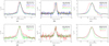 |
Fig. 1 Spectra of H2S 110-101, H234S 110 -101, and H2CS 514-414 detected with IRAM for three sources (a, b and c) and HCS+ 4-3 and SiO 4-3 lines (d, e and f). All of the observed spectra are aligned to the peak of HC3N 19-18. In panels (a), (b), and (c), red lines are H2S 110-101, blue lines are H234S 110-101, and green lines are H2CS 514-414. In (d), (e), and (f), HCS+ 4-3 lines are in green and SiO 4-3 lines are red. The black lines in all panels represent HC3N. |
3 Results
3.1 The detected lines
Lines of H2S 110-101,H234S 110-101,H2CS 514-414, HCS+ 4-3, andHC3N 19-18 were detected in all sources except for G012.90- 00.24, SiO 4-3 was detected in 46 sources, and C18O 1-0 was detected in all sources (see Figures 1 and A.1). The H2S 110- 101 lines are generally stronger than H2CS 514-414, while H2CS 514-414 lines are stronger than HCS+ 4-3. The sources can be divided into three groups based in the line profile of H2S 110- 101 and H234S 110-101. For 26 sources of the sample, including G027.36-00.16 (see Figure 1a), both lines can be fitted with a single Gaussian component, while in 21 sources, including G031.28+00.06 (see Figure 1b), H2S 110-101 needs from two to four components, and this is probably caused by inflowing gas. There are three sources, G049.48-00.38 (W51M, see Figure 1c), G043.16+00.01 (W49N), and G000.67-00.03 (SgrB2), in which there is a possible optically thin velocity component of H2S 110- 101 that does not correspond to H234S 110-101 emission. The column densities of H2S were calculated from those of H234S for all the sources.
We used HC3N 19-18 to confirm the central velocities and line profile of S-bearing lines, and C18O to obtain H2 column densities and thereby the relative H2S, H2CS, and HCS+ abundances. SiO was used as the tracer of shock activities in SFRs.
Table 1 shows the molecular species, velocity-integrated intensities, central velocity, and peak temperature. Velocity- integrated fluxes were obtained from the single-component Gaussian fitting, or with the “print area” for H2S, H2CS, and C18O in CLASS if a complex line profile was found (see Section 2.2; there instances are noted with an “a” superscript in column 4 of Table 1). As shown in Table 1, the velocity- integrated intensities and peak temperature of H2S 110-101 are higher than those of H2CS 514-414, while those of H2CS 514-414 are higher than those of HCS+ 4-3. The S-bearing species studied in this work have similar line widths, while SiO 4-3 has a broader line width than the other lines in each source.
3.2 Column densities
The beam-averaged column densities of H2S, H234S, H2CS, HCS+, SiO, and C18O molecules are shown in Table B.1. The H2S ranges from 3.59 × 10¹³ to 3.50 × 1015cm-2, H234S from 1.65 × 10¹² to 1.83 × 1014cm-2, H2CS from 7.09 × 10¹² to 1.25 × 1015cm−2, and HCS+ from 6.67 × 10¹¹ to 6.04 × 1013cm−2.HCS+ is the lowest abundant molecules among H2S, H2CS and HCS+. The resulting column densities for SiO and C18O molecules in these 50 sources range from 3.33 × 10¹¹ to 9.25 × 1013cm−2 and from 6.30 × 10¹⁵ to 3.76 × 1016cm−2, respectively. The column densities of H2 were derived from C18O as  (Frerking et al. 1982) and range from 1.13 × 10²² to 4.80 × 1023cm−2.
3.3 Relative abundances
The relative abundances of these molecules, which can be obtained with beam-averaged column densities, are more important than the beam-averaged column densities themselves for scientific analyses. The abundances of H2S, H2CS, and HCS+ normalized by H2 are shown in Table D.1; the H2 S abundances were obtained by multiplying H234S abundance by the 32S/34S ratios. The relation between the abundances of H2 S and HCS+ normalized by H2 and determined via least square fitting is presented in Figure 2a; it has a Pearson correlation coefficient3 of 0.76 and a slope of 0.97. Also shown are the abundances of H2S and H2CS normalized by H2 with a Pearson correlation coefficients and slope of 0.77 and 0.98, respectively (see Figure 2b). For the abundances of H2CS and HCS+ normalized by H2 (see Figure 2c), the Pearson correlation coefficients and slope were 0.94 and 1.00. Since the slopes and Pearson correlation coefficients are are positive numbers close to or equal to 1, H2S, H2CS, and HCS+ molecules are probably very closely chemically related to each other.
The relative abundances of H2S, H2CS, and HCS+ normalized by H2 of these 50 sources span more than one order of magnitude. Table E.1 shows the abundance ratios [H2S/H2CS], [H2S/HCS+], and [H2CS/HCS+] toward all the sources. The abundance ratio of: [H2S/H2CS] ranges from 1.32±0.12 in G000.67-00.03 to 10.2 ± 0.49 in G109.87+02.11 with a median value of 4.4; [H2S/HCS+] from 14.1 ± 7.01 in G011.49-01.48 to 129.6 ± 11.1 in G109.87+02.11 with a median value of 63.8; and [H2CS/HCS+] from 7.94 ± 0.61 in G232.62+00.99 to 23.6 ± 0.96 in G049.48-00.36 with a median value of 13.0.
A good correlation is found between H2CS and HCS+ whether normalized by H2S or H2 (see Figures 3 and 2c). The abundance ratios of [H2CS/HCS+] are within a narrower range than that of [H2S/HCS+] and [H2S/H2CS] (see Table E.1). G011.49-01.48 and G0168.06+00.82, with large errors, are marked where H234S lines show weak emission in Figures 2 and 3.
The relationships between S-bearing molecules and SiO, normalized by H2, are shown in Figure 4, with Pearson correlation coefficients of HCS+, H2CS, and H2S with SiO of 0.60, 0.68, and 0.57, and slopes of 0.73, 0.75, and 0.72, respectively. Though the correlations are not as tight as that between the S- bearing molecules themselves (see Figure 2), the abundances of HCS+, H2CS, and H2S increase with the SiO abundance in these sources. Shock chemistry might be needed in further modeling.
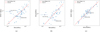 |
Fig. 2 Relationship between the HCS+ and H2S abundances (a), H2CS and H2S abundances (b), and HCS+ and H2CS abundances (c), all normalized by H2. The fitting lines, generated using the least square method, are marked in red. G011.49-01.48 and G0168.06+00.82, which have large errors, are marked where H234S lines show weak emission. |
3.4 Line profiles
In most cases, the lines are very well fitted with a single Gaussian (see Figures 1 and A.1). This is especially apparent in H234S, H2CS, HCS+, and HC3N (except for H2S and SiO). The full widths at half maxima (FWHMs) are similar to each other for the H234S, H2CS, HCS+, and HC3N lines in each source, between 1 km s−1 and 10 km s−1 (see Table C.1), except for G000.67- 00.03 (Sgr B2) and G043.16+000.01 (W49N). Figure 5 shows a comparison of the FWHMs of the observed lines: the correlation between HCS+ and H2CS is perfect, with a Pearson correlation coefficient of 0.98; it is good between H2CS and H234S (0.94), HCS+ and H234S (0.95), and HCS+ and HC3N (0.92). Such results indicate that these observed H234S, H2CS, HCS+, and HC3N transitions trace the same gas.
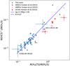 |
Fig. 3 Distribution of the H2CS and HCS+ molecular abundances in each source. Two sources (G011.49-01.48 and G0168.06+00.82) have large errors due to the weak emission of the H234 S lines. The molecular abundance ratios from Fontani et al. (2023) are also presented. |
4 Discussion
4.1 Possible chemical connections between H2S, H2CS, and HCS+ in hot cores?
S-bearing species are good tracers of hot cores because they are particularly sensitive to physical and chemical changes in dense and hot regions (Hatchell et al. 1998). H2S is the main molecular form of S-bearing molecules in molecular clouds, which may be produced on the surface of grains, and the rapid reactions of H2S molecules can drive the production of other S-bearing molecules (Druard & Wakelam 2012). The measured abundances of H2S:H2CS:HCS+ in these 50 sources show that H2S is more abundant than H2CS, and HCS+, and H2O is more abundant than H2CO and HCO+ (Herbst & Klemperer 1973).
With a correlation coefficient of 0.94, the correlation between the abundances of HCS+ and H2CS is tighter than the correlation between either of these two molecules and H2 S (see Figure 2c). This is likely due to different chemical formation processes for H2S compared to HCS+ and H2CS in chemical models. H2S is mainly formed on grain surfaces (Druard & Wakelam 2012), while the other two molecules are primarily formed in the gas phase (Vidal & Wakelam 2018; Gronowski & Kołos 2014). Additionally, the elemental carbon also affects the formation of H2CS and HCS+, which can reflect the better correlation of HCS+ versus H2CS than that of HCS+ versus H2S and H2CS versus H2S in observations. Not only the correlation coefficients, but also the slopes of the fitting results can be used to substantiate the relation between the abundances of the two molecules. We find a tight linear relationship between HCS+ and H2CS, with slope of 1.00; the relation between H2CS and H2S is 0.98, and it is 0.97 for HCS+ and H2S.
Our sample comprises 51 massive late-stage SFRs, while the sample in Fontani et al. (2023) comprises 15 sources at different stages (see Figure 3). The HCS+/H2S versus H2CS/H2S trend found in this work is also found in Fontani et al. (2023). We obtained line widths and excitation temperatures to confirm that HCS+ preferentially traces quiescent and likely extended material. Our results show that the line widths of the H234S, H2CS, HCS+, and HC3N lines in each source are almost the same (see Figure 5), which indicates that they may be from the same gas.
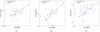 |
Fig. 4 Relationships between the HCS+ and SiO abundances (a), H2CS and SiO abundances (b), and H2S and SiO abundances (c), all normalized by H2. The fitting lines, generated using the least square method, are marked in red. The four points marked with red arrows are realistic upper limits of SiO and were not used in the fitting. |
 |
Fig. 5 Comparison of the line FWHMs of the observed species. In all plots, the two distant blue points with red circles represent G000.67-00.03 (Srg B2) and G043.16+00.01 (W49N). The number in the upper-left corner of each panel is the Pearson correlation coefficient, ρ. The gray line is y=x. The ratios from Bouvier et al. (2024) and Fontani et al. (2023) are also presented. |
4.2 Chemical model including gas, dust grain surface and icy mantle phases, for H2S, H2CS, and HCS+
To better understand the observed abundances of H2S, H2CS, and HCS+ in hot cores, we utilized the three-phase NAUTILUS chemical code (Ruaud et al. 2016), which takes the gas, dust grain surface, and icy mantle into consideration. We combined it with a similar physical model from Zhang et al. (2023), in which a collapse stage is followed by a warm-up stage. During the collapse stage, the gas density was initially set to 3 × 103 cm−3 and gradually increased to the final density of 1.6 × 107 cm−3 over a period of 1 × 10⁶ years. The gas temperatures were fixed to 10 K during this stage. The density gradually increases over time, resulting in an increase in extinction, as shown in the left panel of Fig. 6. Once the peak density was achieved, the density was fixed and the gas and dust temperatures were raised from ~10 K to their peak temperatures in 2 × 10⁵ years during the warm-up stages, as shown in the right panel of Fig. 6. The main physical parameters of hot core models are summarized in Table 3. For our simulations, we used initial abundances from Table 1 of Vidal & Wakelam (2018). The chemical network is based on the research of Vidal et al. (2017).
In the warm-up stage, H2S is mainly formed through the following hydrogenation reactions on grain surfaces:
 (5)
(5)
Some H2S is already released back into the gas phase through reactive desorption before the temperature rises. When the temperature reaches high values after 2 × 10⁵ yr, it can return to the gas phase through a thermal process, which plays a dominant role in the production of gaseous H2S. Initially, H2S is mainly destroyed by H3+ via ion-neutral reactions in all cases. However, after 2 × 10⁵ yr, 7 × 10⁵ yr, and 3 × 10⁵ yr, it is mainly destructed by atomic carbon for a Tmax of 60 and 100 K and by atomic hydrogen for a Tmax of 150 K in the gas phase, respectively. The related reactions are as follows:
 (6)
(6)
H2CS is primarily formed in the gas phase through the following neutral-neutral reaction:
 (7)
(7)
and it follows a similar destruction pathway as H2S, as both are initially broken down through the ion H3+. After 5 × 10⁵ yr, 7 × 10⁵ yr, and 9 × 10⁵ yr in the gas phase, it is mainly destroyed by atomic carbon for Tmax of 60, 100, and 150 K, respectively. The reactions proceed as follows:
 (8)
(8)
Initially, HCS+ is mainly formed through the reaction ofCS with the H3+ ion in all cases. However, after 3 × 10⁵ yr and 7 × 10⁵ yr, it is primarily produced via the reactions CS + HCO+ and CS + HCNH+ for Tmax of 60 and 150 K, respectively. The related reactions are as follows:
 (9)
(9)
It is mainly destroyed in the gas phase via the following electron recombination:
 (10)
(10)
Both H2S and H2CS can be destroyed via reactions with H3+ (see Eqs. (6) and (8)). The main formation path of HCS+ is a reaction with H3+ (see Eq. (9)). The relations of H2S, H2CS, and HCS+ with H3+ can cause a close connection between them.
Like other similar O-bearing species, H2CO could be produced from H2O+CO, and is the second most abundant product after CO2, at different concentrations of H2O:CO mixtures (de Barros et al. 2022). Other processes can form H2CO from H2O, such as H2O+C→ H2CO at temperatures associated with the ISM and in the cooler regions around young stars (Potapov et al. 2021). This shows that H2CO is formed in a different way with H2CS. The formation of HCO+ under different Av is different. From Av ~ 0.4 to 3, the dominant reaction is CO+ + H2, while above 3, the dominant reaction is H3+ + CO in molecular clouds (Panessa et al. 2023). HCO+ can be destroyed by C3H2 (Narita et al. 2024). The formation paths of HCO+ and HCS+ seem to be the same in particular cases.
The model results of the relative abundances of H2S, H2CS, and HCS+ species in the gas phase varying with time in warmup stages are presented in Figure 7 with three different maximum temperatures (Tmax): 604, 100, and 150 K. The measured abundances are compared with the abundances from the model, which can have the same value at different times (see Figure 7). The samples are in the same evolutionary stage, and the more reasonable intersections are marked, as are other possible times. We considered the calculated abundance to be consistent with the observed value if the calculated abundance differs from the observed value by less than one order of magnitude.
For Tmax=60 K (see Figure 7, red lines), the abundance of H2S and H2CS varies much less than that of HCS+. Additionally, there is one possible time (3× 10⁵ yr) for each source that matchs the measured [H2CS/H2] and [HCS+/H2] abundances (see Figures 7a and 7b, red line and filled circles) and no intersection for [H2S/H2] (see Figure 7c). However, the discrepancy is less than one order of magnitude. The overprediction of H2S that we find relative to the observational results could be a result of the absence of effective gas-phase destruction reactions in the H2S chemistry within our model. [HCS+/H2] abundances in all sources range from 1.84 × 10⁻¹¹ to 3.54 × 10⁻¹⁰, and four of them rang from 2.19 × 10⁻¹⁰ to 3.54 × 10⁻¹⁰, which is higher than the model results (see Figure 7b, orange filled rectangle). All sources with measured [H2CS/H2] abundances, which range from 2.94 × 10⁻¹⁰ to 4.15 × 10⁻⁹, match the model results.
The abundances of H2CS and HCS+ change more quickly than H2S, in 1 × 10⁵ to 1 × 10⁷ yr, with Tmax =100 K (see Figure 7, blue lines). There is not a single time in common between the observed value and the model. The solutions are totally different for different molecules (see Figure 7), with about 2×10⁵ yr for [H2CS/H2], 3×10⁵ yr for [HCS+/H2], and 5×10⁵ yr for [H2S/H2].
The possible times with Tmax=150K for each source to match the measured abundances of [H2S/H2] are concentrated around 3 × 10⁵ yr (see Figure 7c, green lines). Of the two to four possible time solutions for [H2CS/H2] and [HCS+/H2], the earliest is the most likely for most sources; one time is shared by the different abundances in each source, around 3 × 10⁵ yr.
In general, the models can reproduce the observed abundances at around 2-3 × 10⁵ yr for almost all of the sources. However, there is a small discrepancy for lower-Tmax (60 K) models of H2S. H2CS and HCS+ can be efficiently formed in the gas phase, while H2S already chemically desorbs during its formation on the grains before being thermally desorbed. The abundance of H2S cannot sharply increase like at the Tmax of 100 and 150 K after the temperature reaches Tmax of 60 K because it does not reach the desorption temperature of H2S (around 70 K). In this condition, the chemical desorption is the primary origin for gaseous H2S. Since gas-phase destruction reactions for H2S are not as effective at the relatively low temperature of 60 K (compared to the Tmax of 100 and 150 K), the abundance of H2S is overpredicted in our model.
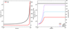 |
Fig. 6 Density, temperature, and AV profiles as functions of time for collapse and warm-up stages in hot core models. Left: collapse stage. The gas density gradually increases from 3 × 103 cm−3 to 1.6 × 107 cm−3 over a period of 1 × 10⁶ years, and the temperature remains at a constant value of 10 K. An increase in gas density leads to an increase in visual extinction. Right: warm-up stage. The gas density and visual extinction are 1.6 × 107 cm−3 and 6.109 × 10² mag, respectively; we used three values for Tmax: 60, 100 and 150 K. |
Physical parameters of hot core models.
 |
Fig. 7 Chemical model including the gas, the dust grain surface and the icy mantle. The solid lines correspond to the gas-phase abundances versus time during warm-up stages in chemical models with gas maximum temperatures of 60, 100, and 150 K, and the points are the observed data. The abundances of H2CS, HCS+ and H2S relative to H2 are presented in panels (a), (b), and (c), respectively. Since the samples are in the same evolutionary stage, two possible times from the form model are marked, with filled and transparent circles. Note that there are no intersections for H2S at 60 K in model. |
4.3 Shock activities
SiO is considered to be an excellent tracer of shock activities in SFRs because the SiO abundance in molecular outflows is at least three orders of magnitude higher than in quiescent gas (Schilke et al. 1997). Lots of elemental Si is probably in the form of stable materials in dust, like silicates, and is effectively trapped. Shock activities is needed to destroy silicates to release Si atoms from grains into the gas phase (Martin-Pintado et al. 1992), and the abundance of S-bearing molecules can be increased via moderate shocks (Wakelam et al. 2004).
SiO 4-3 was detected in 46 of the 51 sources in our sample (see the green lines in Figures 1 d–f), which indicates shock activities. The abundances of HCS+, H2CS, and H2S increase with the SiO abundance in these sources (see Figure 4), which implies that shock chemistry is important for HCS+, H2CS, and H2S. In addition, the line width of SiO is larger than those of the S-bearing species. This indicates that the SiO is actually tracing a different physical component with a different velocity broadening. SiO likely traces shocked regions, which implies that the S-bearing species are either tracing weaker shocks not traced by SiO or are actually tracing the hot core regions.
5 Summary and conclusions
We observed H2S 110-101, H234S 110-101, H2CS 514-414, HCS+ 4-3, HC3N 19-18, SiO 4-3, and C18O 1-0 toward a sample of 51 massive SFRs with the IRAM 30 m telescope. We derived beam average column densities, as well as their abundances with respect to H2, from C18O.
All lines can be well fitted with a single Gaussian, except for H2S and SiO. The FWHMs are between 1 km s−1 and 10 km s−1 in all sources, except for G000.67-00.03 (Sgr B2) and G043.16+00.01 (W49N). The line FWHMs of the observed species are positively correlated with each other and have similar ranges, which indicates that they may trace similar regions.
The abundance ratios of [H2S/H2], [H2CS/H2], and [HCS+/H2] range by more than one magnitude with high correlation coefficients and positive slopes: a correlation coefficient of 0.94 and a slope of 1.00 for [H2CS/H2] and [HCS+/H2], and 0.76 and 0.97 for [H2S/H2] and [HCS+/H2]. For [H2CS/H2] and [H2S/H2] the correlation coefficients and slope are 0.77 and 0.98. These close relations indicate that these S-bearing molecules may have chemical connections with each other, with HCS+ and H2CS the most correlated based on the relations between the relative abundances of these molecules and those of the other 50 sources.
The three-phase NAUTILUS chemical code was utilized to simulate the relationship of three S-bearing molecules. Comparing the results of observation and model, we find one possible time (2–3 × 10⁵ yr) at which each source in the model matches the measured abundances of H2S, H2CS, and HCS+. The abundances of HCS+, H2CS, and H2S increase with the SiO abundance in these sources, which implies that shock chemistry may be important for them. Shock activity needs to be considered in further modeling of H2S, H2CS, and HCS+ in hot cores.
Data availability
More information about H2S 110-101, H234S 110-101, H2CS 514-414, HCS+ 4-3, HC3N 19-18, SiO 4-3, and C18O 1-0 lines from our sample is available on Zenodo under the following link: https://doi.org/10.5281/zenodo.13937627
Acknowledgements
R.L., J.Z.W., Y.N.X., and C.O. are supported by National Key R&D Program of China (2023YFA1608204) and the National Natural Science Foundation of China grant 12173067. D.H.Q. and X.J.J. are supported by the National Natural Science Foundation of China (Grant No. 12373026), the Leading Innovation and Entrepreneurship Team of Zhejiang Province of China (Grant No. 2023R01008), and the Key R&D Program of Zhejiang, China (Grant No. 2024SSYS0012). This study is based on observations carried out under project number 012-16, 023-17 and 005-20 with the IRAM 30 m telescope. IRAM is supported by INSU/CNRS (France), MPG (Germany) and IGN (Spain).
Appendix A Spectra for individual sources
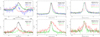 |
Fig. A.1 Same as Figure 1 but for more sources. Additional figures are available on Zenodo. https://doi.org/10.5281/zenodo.13937627 |
Appendix B Beam-averaged column densities
Beam-averaged column densities.
Appendix C The line widths at half maximum of the molecules
Line widths at half maximum of the molecules in km s−1.
Appendix D 32S/34S ratios,  , and abundances
Information on the 32S/34S ratios,  , and abundances.
Appendix E Abundance ratios
Abundance ratios of S-bearing molecules.
References
- Adande, G. R., Halfen, D. T., Ziurys, L. M., et al. 2010, ApJ, 725, 561 [NASA ADS] [CrossRef] [Google Scholar]
- Asplund, M., Grevesse, N., & Sauval, A. J. 2005, ASP Conf. Ser., 336, 25 [Google Scholar]
- Blake, G. A., Sutton, E. C., Masson, C. R., et al. 1987, ApJ, 315, 621 [NASA ADS] [CrossRef] [Google Scholar]
- Bonfand, M., Belloche, A., Garrod, R. T., et al. 2019, A&A, 628, A27 [NASA ADS] [CrossRef] [EDP Sciences] [Google Scholar]
- Bouscasse, L., Csengeri, T., Belloche, A., et al. 2022, A&A, 662, A32 [NASA ADS] [CrossRef] [EDP Sciences] [Google Scholar]
- Bouvier, M., Viti, S., Behrens, E., et al. 2024, A&A, 689, A64 [NASA ADS] [CrossRef] [EDP Sciences] [Google Scholar]
- Brown, R. D., Godfrey, P. D., & Winkler, D. A. 1980, MNRAS, 190, 1 [NASA ADS] [CrossRef] [Google Scholar]
- Cernicharo, J., Guélin, M., & Kahane, C. 2000, A&AS, 142, 181 [NASA ADS] [CrossRef] [EDP Sciences] [Google Scholar]
- Charnley, S. B. 1997, ApJ, 481, 396 [NASA ADS] [CrossRef] [Google Scholar]
- Chin, Y.-N., Henkel, C., Whiteoak, J. B., et al. 1996, A&A, 305, 960 [NASA ADS] [Google Scholar]
- Coutens, A., Willis, E. R., Garrod, R. T., et al. 2018, A&A, 612, A107 [NASA ADS] [CrossRef] [EDP Sciences] [Google Scholar]
- Drdla, K., Knapp, G. R., & van Dishoeck, E. F. 1989, ApJ, 345, 815 [Google Scholar]
- Druard, C., & Wakelam, V. 2012, MNRAS, 426, 354 [NASA ADS] [CrossRef] [Google Scholar]
- de Barros, A. L. F., Mejía, C., Seperuelo Duarte, E., et al. 2022, MNRAS, 511, 2491 [Google Scholar]
- el Akel, M., Kristensen, L. E., Le Gal, R., et al. 2022, A&A, 659, A100 [CrossRef] [EDP Sciences] [Google Scholar]
- Esplugues, G. B., Tercero, B., Cernicharo, J., et al. 2013, A&A, 556, A143 [NASA ADS] [CrossRef] [EDP Sciences] [Google Scholar]
- Esplugues, G. B., Viti, S., Goicoechea, J. R., et al. 2014, A&A, 567, A95 [NASA ADS] [CrossRef] [EDP Sciences] [Google Scholar]
- Esplugues, G., Fuente, A., Navarro-Almaida, D., et al. 2022, A&A, 662, A52 [NASA ADS] [CrossRef] [EDP Sciences] [Google Scholar]
- Esplugues, G., Rodríguez-Baras, M., San Andrés, D., et al. 2023, A&A, 678, A199 [NASA ADS] [CrossRef] [EDP Sciences] [Google Scholar]
- Frerking, M. A., Linke, R. A., & Thaddeus, P. 1979, ApJ, 234, L143 [NASA ADS] [CrossRef] [Google Scholar]
- Frerking, M. A., Langer, W. D., & Wilson, R. W. 1982, ApJ, 262, 590 [Google Scholar]
- Fontani, F., Roueff, E., Colzi, L., et al. 2023, A&A, 680, A58 [NASA ADS] [CrossRef] [EDP Sciences] [Google Scholar]
- Garozzo, M., Fulvio, D., Kanuchova, Z., et al. 2010, A&A, 509, A67 [NASA ADS] [CrossRef] [EDP Sciences] [Google Scholar]
- Garrod, R. T., & Herbst, E. 2006, A&A, 457, 927 [NASA ADS] [CrossRef] [EDP Sciences] [Google Scholar]
- Goldsmith, P. F., & Linke, R. A. 1980, ApJ, 81, 30064 [Google Scholar]
- Goldsmith, P. F., & Langer, W. D. 1999, ApJ, 517, 209 [Google Scholar]
- Gronowski, M., & Kolos, R. 2014, ApJ, 792, 89 [NASA ADS] [CrossRef] [Google Scholar]
- Gottlieb, C. A., Gottlieb, E. W., Litvak, M. M., et al. 1978, ApJ, 219, 77 [NASA ADS] [CrossRef] [Google Scholar]
- Gudeman, C. S., Haese, N. N., Piltch, N. D., et al. 1981, ApJ, 246, L47 [NASA ADS] [CrossRef] [Google Scholar]
- Hatchell, J., Thompson, M. A., Millar, T. J., et al. 1998, A&A, 338, 713 [NASA ADS] [Google Scholar]
- Herbst, E., & Klemperer, W. 1973, ApJ, 185, 505 [Google Scholar]
- Inostroza-Pino, N., Palmer, C. Z., Lee, T. J., et al. 2020, J. Mol. Spectrosc., 369, 111273 [NASA ADS] [CrossRef] [Google Scholar]
- Jenkins, E. B. 2009, ApJ, 700, 1299 [Google Scholar]
- Jiménez-Escobar, A., & Muñoz Caro, G. M. 2011, A&A, 536, A91 [Google Scholar]
- Kalenskii, S. V., Slysh, V. I., & Val’tts, I. E. 2002, Astron. Rep., 46, 96 [NASA ADS] [CrossRef] [Google Scholar]
- Kalenskii, S. V., Kaiser, R. I., Bergman, P., et al. 2022, ApJ, 932, 5 [NASA ADS] [CrossRef] [Google Scholar]
- Li, J., Wang, J., Zhu, Q., et al. 2015, ApJ, 802, 40 [NASA ADS] [CrossRef] [Google Scholar]
- Li, Y., Wang, J., Li, J., et al. 2022, MNRAS, 512, 4934 [NASA ADS] [CrossRef] [Google Scholar]
- Lis, D. C., Goldsmith, P. F., Güsten, R., et al. 2023, A&A, 669, L15 [NASA ADS] [CrossRef] [EDP Sciences] [Google Scholar]
- Luo, G., Feng, S., Li, D., et al. 2019, ApJ, 885, 82 [NASA ADS] [CrossRef] [Google Scholar]
- Martin-Pintado, J., Bachiller, R., & Fuente, A. 1992, A&A, 254, 315 [NASA ADS] [Google Scholar]
- McClure, M. K., Rocha, W. R. M., Pontoppidan, K. M., et al. 2023, Nat. Astron., 7, 431 [NASA ADS] [CrossRef] [Google Scholar]
- Miessler, G. L., Fischer, P. J., & Tarr, D. A. 2013, Inorganic Chemistry, 5th edn., (london: Pearson) [Google Scholar]
- Minh, Y. C., Ziurys, L. M., Irvine, W. M., et al. 1991, ApJ, 366, 192 [NASA ADS] [CrossRef] [Google Scholar]
- Montaigne, H., Geppert, W. D., Semaniak, J., et al. 2005, ApJ, 631, 653 [NASA ADS] [CrossRef] [Google Scholar]
- Müller, H. S. P., Thorwirth, S., Roth, D. A., et al. 2001, A&A, 370, L49 [Google Scholar]
- Müller, H. S. P., Schlöder, F., Stutzki, J., et al. 2005, J. Mol. Struc., 742, 215 [CrossRef] [Google Scholar]
- Navarro-Almaida, D., Le Gal, R., Fuente, A., et al. 2020, A&A, 637, A39 [NASA ADS] [CrossRef] [EDP Sciences] [Google Scholar]
- Narita, K., Sakamoto, S., Koda, J., et al. 2024, ApJ, 969, 102 [NASA ADS] [CrossRef] [Google Scholar]
- Neufeld, D. A., Godard, B., Gerin, M., et al. 2015, A&A, 577, A49 [NASA ADS] [CrossRef] [EDP Sciences] [Google Scholar]
- Panessa, M., Seifried, D., Walch, S., et al. 2023, MNRAS, 523, 6138 [NASA ADS] [CrossRef] [Google Scholar]
- Potapov, A., Krasnokutski, S. A., Jäger, C., et al. 2021, ApJ, 920, 111 [CrossRef] [Google Scholar]
- Reid, M. J., Menten, K. M., Brunthaler, A., et al. 2014, ApJ, 783, 130 [Google Scholar]
- Reid, M. J., Pesce, D. W., & Riess, A. G. 2019, ApJ, 886, L27 [Google Scholar]
- Ruaud, M., Wakelam, V., & Hersant, F. 2016, MNRAS, 459, 3756 [Google Scholar]
- Santos, J. C., Linnartz, H., & Chuang, K.-J. 2023, A&A, 678, A112 [NASA ADS] [CrossRef] [EDP Sciences] [Google Scholar]
- Schilke, P., Walmsley, C. M., Pineau des Forets, G., et al. 1997, A&A, 321, 293 [Google Scholar]
- Schwartz, P. R., Zuckerman, B., & Bologna, J. M. 1982, ApJ, 256, L55 [NASA ADS] [CrossRef] [Google Scholar]
- Shingledecker, C. N., Lamberts, T., Laas, J. C., et al. 2020, ApJ, 888, 52 [Google Scholar]
- Thaddeus, P., Kutner, M. L., Penzias, A. A., et al. 1972, ApJ, 176, L73 [NASA ADS] [CrossRef] [Google Scholar]
- Turner, B. E. 1989, ApJS, 70, 539 [NASA ADS] [CrossRef] [Google Scholar]
- Tychoniec, L., van Dishoeck, E. F., van’t Hoff, M. L. R., et al. 2021, A&A, 655, A65 [NASA ADS] [CrossRef] [EDP Sciences] [Google Scholar]
- Ulich, B. L., & Haas, R. W. 1976, ApJS, 30, 247 [Google Scholar]
- van der Tak, F. F. S., Black, J. H., Schöier, F. L., et al. 2007, A&A, 468, 627 [NASA ADS] [CrossRef] [EDP Sciences] [Google Scholar]
- van Dishoeck, E. F., Kristensen, L. E., Mottram, J. C., et al. 2021, A&A, 648, A24 [NASA ADS] [CrossRef] [EDP Sciences] [Google Scholar]
- Vidal, T. H. G., & Wakelam, V. 2018, MNRAS, 474, 5575 [Google Scholar]
- Vidal, T. H. G., Loison, J.-C., Jaziri, A. Y., et al. 2017, MNRAS, 469, 435 [Google Scholar]
- Wakelam, V., Castets, A., Ceccarelli, C., et al. 2004, A&A, 413, 609 [NASA ADS] [CrossRef] [EDP Sciences] [Google Scholar]
- Yan, Y. T., Henkel, C., Kobayashi, C., et al. 2023, A&A, 670, A98 [NASA ADS] [CrossRef] [EDP Sciences] [Google Scholar]
- Zhang, X., Quan, D., Li, R., et al. 2023, MNRAS, 521, 1578 [NASA ADS] [CrossRef] [Google Scholar]
The Pearson correlation coefficient is a measure of the linear relationship between two variables. The closer |γ| is to 1, the stronger the linear relationship.
All Tables
All Figures
|
Fig. 1 Spectra of H2S 110-101, H234S 110 -101, and H2CS 514-414 detected with IRAM for three sources (a, b and c) and HCS+ 4-3 and SiO 4-3 lines (d, e and f). All of the observed spectra are aligned to the peak of HC3N 19-18. In panels (a), (b), and (c), red lines are H2S 110-101, blue lines are H234S 110-101, and green lines are H2CS 514-414. In (d), (e), and (f), HCS+ 4-3 lines are in green and SiO 4-3 lines are red. The black lines in all panels represent HC3N. |
| In the text | |
|
Fig. 2 Relationship between the HCS+ and H2S abundances (a), H2CS and H2S abundances (b), and HCS+ and H2CS abundances (c), all normalized by H2. The fitting lines, generated using the least square method, are marked in red. G011.49-01.48 and G0168.06+00.82, which have large errors, are marked where H234S lines show weak emission. |
| In the text | |
|
Fig. 3 Distribution of the H2CS and HCS+ molecular abundances in each source. Two sources (G011.49-01.48 and G0168.06+00.82) have large errors due to the weak emission of the H234 S lines. The molecular abundance ratios from Fontani et al. (2023) are also presented. |
| In the text | |
|
Fig. 4 Relationships between the HCS+ and SiO abundances (a), H2CS and SiO abundances (b), and H2S and SiO abundances (c), all normalized by H2. The fitting lines, generated using the least square method, are marked in red. The four points marked with red arrows are realistic upper limits of SiO and were not used in the fitting. |
| In the text | |
|
Fig. 5 Comparison of the line FWHMs of the observed species. In all plots, the two distant blue points with red circles represent G000.67-00.03 (Srg B2) and G043.16+00.01 (W49N). The number in the upper-left corner of each panel is the Pearson correlation coefficient, ρ. The gray line is y=x. The ratios from Bouvier et al. (2024) and Fontani et al. (2023) are also presented. |
| In the text | |
|
Fig. 6 Density, temperature, and AV profiles as functions of time for collapse and warm-up stages in hot core models. Left: collapse stage. The gas density gradually increases from 3 × 103 cm−3 to 1.6 × 107 cm−3 over a period of 1 × 10⁶ years, and the temperature remains at a constant value of 10 K. An increase in gas density leads to an increase in visual extinction. Right: warm-up stage. The gas density and visual extinction are 1.6 × 107 cm−3 and 6.109 × 10² mag, respectively; we used three values for Tmax: 60, 100 and 150 K. |
| In the text | |
|
Fig. 7 Chemical model including the gas, the dust grain surface and the icy mantle. The solid lines correspond to the gas-phase abundances versus time during warm-up stages in chemical models with gas maximum temperatures of 60, 100, and 150 K, and the points are the observed data. The abundances of H2CS, HCS+ and H2S relative to H2 are presented in panels (a), (b), and (c), respectively. Since the samples are in the same evolutionary stage, two possible times from the form model are marked, with filled and transparent circles. Note that there are no intersections for H2S at 60 K in model. |
| In the text | |
|
Fig. A.1 Same as Figure 1 but for more sources. Additional figures are available on Zenodo. https://doi.org/10.5281/zenodo.13937627 |
| In the text | |
Current usage metrics show cumulative count of Article Views (full-text article views including HTML views, PDF and ePub downloads, according to the available data) and Abstracts Views on Vision4Press platform.
Data correspond to usage on the plateform after 2015. The current usage metrics is available 48-96 hours after online publication and is updated daily on week days.
Initial download of the metrics may take a while.