| Issue |
A&A
Volume 691, November 2024
|
|
|---|---|---|
| Article Number | A185 | |
| Number of page(s) | 25 | |
| Section | Extragalactic astronomy | |
| DOI | https://doi.org/10.1051/0004-6361/202348897 | |
| Published online | 18 November 2024 | |
Constraining the giant radio galaxy population with machine learning and Bayesian inference
1
Leiden Observatory, Leiden University, PO Box 9513 2300 RA Leiden, The Netherlands
2
ASTRON, the Netherlands Institute for Radio Astronomy, Oude Hoogeveensedijk 4, 7991 PD Dwingeloo, The Netherlands
3
Cahill Center for Astronomy and Astrophysics, California Institute of Technology, 1216 E California Blvd, Pasadena, 91125 CA, USA
4
School of Physical Sciences, The Open University, Walton Hall, Milton Keynes MK7 6AA, UK
5
Institute for Astronomy, Royal Observatory, Blackford Hill, Edinburgh EH9 3HJ, UK
6
Centre for Astrophysics Research, Department of Physics, Astronomy and Mathematics, University of Hertfordshire, College Lane, Hatfield AL10 9AB, UK
⋆⋆ Corresponding authors; This email address is being protected from spambots. You need JavaScript enabled to view it.
; This email address is being protected from spambots. You need JavaScript enabled to view it.
Received:
10
December
2023
Accepted:
23
February
2024
Abstract
Context. Large-scale sky surveys at low frequencies, such as the LOFAR Two-metre Sky Survey (LoTSS), allow for the detection and characterisation of unprecedented numbers of giant radio galaxies (GRGs, or “giants”, of at least lp, GRG := 0.7 Mpc long). This, in turn, enables us to study giants in a cosmological context. A tantalising prospect of such studies is a measurement of the contribution of giants to cosmic magnetogenesis. However, this measurement requires en masse radio–optical association for well-resolved radio galaxies and a statistical framework to infer GRG population properties.
Aims. By automating the creation of radio–optical catalogues, we aim to significantly expand the census of known giants. With the resulting sample and a forward model that takes into account selection effects, we aim to constrain their intrinsic length distribution, number density, and lobe volume-filling fraction (VFF) in the Cosmic Web.
Methods. We combined five existing codes into a single machine learning (ML)–driven pipeline that automates radio source component association and optical host identification for well-resolved radio sources. We created a radio–optical catalogue for the entire LoTSS Data Release 2 (DR2) footprint and subsequently selected all sources that qualify as possible giants. We combined the list of ML pipeline GRG candidates with an existing list of LoTSS DR2 crowd-sourced GRG candidates and visually confirmed or rejected all members of the merged sample. To infer intrinsic GRG properties from GRG observations, we developed further a population-based forward model and constrained its parameters using Bayesian inference.
Results. Roughly half of all GRG candidates that our ML pipeline identifies indeed turn out to be giants upon visual inspection, whereas the success rate is 1 in 11 for the previous best giant-finding ML technique in the literature. We confirm 5576 previously unknown giants from the crowd-sourced LoTSS DR2 catalogue and 2566 previously unknown giants from the ML pipeline. Our confirmations and discoveries bring the total number of known giants to at least 11 485. Our intrinsic GRG population forward model provides a good fit to the data. The posterior indicates that the projected lengths of giants are consistent with a curved power law probability density function whose initial tail index ξ(lp, GRG) = − 2.8 ± 0.2 changes by Δξ = −2.4 ± 0.3 over the interval up to lp = 5 Mpc. We predict a comoving GRG number density nGRG = 13 ± 10 (100 Mpc)−3, close to a recent estimate of the number density of luminous non-giant radio galaxies. With the projected length distribution, number density, and additional assumptions, we derive a present-day GRG lobe VFF 𝒱GRG − CW(z = 0) = 1.4 ± 1.1 × 10⁻⁵ in clusters and filaments of the Cosmic Web.
Conclusions. We present a state-of-the-art ML-accelerated pipeline for finding giants, whose complex morphologies, arcminute extents, and radio-emitting surroundings pose challenges. Our data analysis suggests that giants are more common than previously thought. More work is needed to make GRG lobe VFF estimates reliable, but tentative results imply that it is possible that magnetic fields once contained in giants pervade a significant (≳10%) fraction of today’s Cosmic Web.
Key words: methods: data analysis / catalogs / surveys / galaxies: active / cosmology: observations / radio continuum: galaxies
These authors contributed equally to this article.
© The Authors 2024
 Open Access article, published by EDP Sciences, under the terms of the Creative Commons Attribution License (https://creativecommons.org/licenses/by/4.0), which permits unrestricted use, distribution, and reproduction in any medium, provided the original work is properly cited.
This article is published in open access under the Subscribe to Open model. This email address is being protected from spambots. You need JavaScript enabled to view it. to support open access publication.
1. Introduction
Recent radio Stokes I imaging and rotation measure observations show that filaments of the Cosmic Web are magnetised (e.g. Govoni et al. 2019; de Jong et al. 2022; Carretti et al. 2023) with B ∼ 100 − 102 nG (e.g. Vazza et al. 2021). However, the origin of these magnetic fields remains highly uncertain. In a primordial magnetogenesis scenario (e.g. Subramanian 2016), the seeds of intergalactic magnetic fields can be traced to the Early Universe. This scenario is not problem-free: primordial magnetic fields that arise before the end of inflation are typically too weak to match observations, while fields that arise after inflation (but before recombination) typically have coherence lengths that are too small. Alternatively, in an astrophysical magnetogenesis scenario, the seeds of intergalactic magnetic fields are predominantly spread by energetic astrophysical phenomena in the more recent Universe, such as radio galaxies (RGs) and supernova-driven winds (e.g. Vazza et al. 2017). In this latter scenario, giant radio galaxies (GRGs, or “giants”) may play a significant role in the magnetisation of the intergalactic medium (IGM), as their associated jets can carry magnetic fields of strength B ∼ 102 nG from host galaxies to cosmological, megaparsec-scale distances (e.g. Oei et al. 2022).
Efforts to measure the contribution of giants to astrophysical magnetogenesis in filaments of the Cosmic Web have only recently begun, with the advent of systematically processed, sensitive, low-frequency sky surveys such as the Low Frequency Array (LOFAR; van Haarlem et al. 2013) Two-metre Sky Survey (LoTSS; Shimwell et al. 2017). By carrying out both a manual search for giants in LoTSS DR2 (Shimwell et al. 2022) pipeline products and a rigorous statistical analysis, Oei et al. (2023a) inferred a key statistic: the volume-filling fraction (VFF) of GRG lobes within clusters and filaments of the Local Universe, 𝒱GRG − CW(z = 0). However, much uncertainty remains as to its value, which is set by the GRG number density, GRG length distribution, and GRG length–lobe volume relation.
As the number of observed radio galaxies rapidly increases with decreasing angular length, the time required to manually associate radio source components and identify host galaxies in the optical logically increases. Machine learning (ML)–based methods have the potential to massively accelerate the detection of various radio source classes by complementing and eventually replacing manual methods (e.g. Proctor 2016; Gheller et al. 2018; Lochner & Bassett 2021; Mostert et al. 2023). The potential for detecting giants was demonstrated by Dabhade et al. (2020a), who visually inspected the 1600 ML-identified GRG candidates of Proctor (2016) and thereby discovered 151 giants. By combining into a single pipeline multiple ML-based and rule-based algorithms that automate both the radio component association and the optical host galaxy identification, we aim to improve upon the 9% precision of Proctor (2016)’s ML predictions.
As part of the present study, we constructed a LoTSS DR2 GRG sample of unparalleled size, by combining results from a visual search by astronomers (Oei et al. 2023a), a visual search by citizen scientists (Hardcastle et al. 2023), and a ML-accelerated search (this article; Sect. 4). With a definitive LoTSS DR2 GRG sample in hand, we refined the Bayesian forward model presented in Oei et al. (2023a), and finally constrained several key geometric quantities pertaining to giants.
In Sect. 2, we briefly review, generalise, and develop the statistical GRG geometry theory of Oei et al. (2023a). In Sect. 3, we introduce the LoTSS DR2 data in which we searched for giants. In Sect. 4, we describe the methods that we used to build our definite LoTSS DR2 GRG sample, and explain how we used the theory of Sect. 2 in practice to infer GRG quantities of interest. In Sect. 5, we present our findings regarding the projected proper length distribution for giants, their comoving number density, and their instantaneous lobe VFF in clusters and filaments of the Cosmic Web. In Sect. 6, we discuss caveats of the present work, compare our results with previous results, and propose directions for future work, before we conclude in Sect. 7.
We assume a flat ΛCDM model with parameters from Planck Collaboration VI (2020): h = 0.6766, ΩBM, 0 = 0.0490, ΩM, 0 = 0.3111, and ΩΛ, 0 = 0.6889, where H0 := h ⋅ 100 km s−1 Mpc−1. We define giants as radio galaxies with a projected proper1 length lp ≥ lp, GRG := 0.7 Mpc. We define the spectral index α such that it relates to flux density Fν at frequency ν as Fν ∝ να; under this convention, α < 0 at radio frequencies for which synchrotron self-absorption is negligible.
2. Theory
To infer the intrinsic length distribution, number density, and lobe VFF of giants, we used a Bayesian forward modelling approach that incorporates selection effects. We adopt the framework described in Oei et al. (2023a), but generalise a few key formulae. Furthermore, in a change that allows for the extraction of tighter parameter constraints from the data, we now predict joint projected proper length–redshift histograms rather than projected proper length distributions.
2.1. RG total and projected proper lengths
The central geometric quantity predicted by models of radio galaxy evolution (e.g. Turner & Shabala 2015; Hardcastle 2018) is, simply, the RG’s intrinsic proper length l. Once the probability distribution of the intrinsic proper length random variable (RV) L is known, one can estimate other geometric quantities of interest, such as the VFF of RG lobes in the Cosmic Web. However, for the vast majority of observed RGs only a projected proper length lp is available, as accurate measurements of jet inclination angles θ are currently challenging. In order to fit statistical models to data from surveys such as LoTSS DR2, models should therefore predict the distribution of the projected proper length RV Lp.
2.2. GRG projected proper length: General
We now show, first without adopting a specific parametric form for the distribution of L, how the cumulative density function (CDF) and probability density function (PDF) of the GRG projected proper length RV Lp | Lp ≥ lp, GRG can be calculated. In particular, we suppose that L has support from some length lmin ≥ 0 onwards. Then Lp = L sinΘ, where Θ is the inclination angle RV. Assuming that, at least on cosmological scales, all RG orientations in three dimensions are equally likely2, the CDF of Lp relates to the PDF of L via
 (1)
(1)
We note that, in the usual scenario of lmin = 0, the second case disappears. Equation (1) generalises Eq. (A.8) from Oei et al. (2023a); its derivation closely follows the one presented there.
The CDF of the GRG projected proper length RV Lp | Lp ≥ lp, GRG is
 (2)
(2)
This result follows from combining Eq. (1) and Eq. (A.12) from Oei et al. (2023a)3. As PDFs follow from CDFs by differentiation, we find that the PDFs of Lp and Lp | Lp ≥ lp, GRG are related by
 (3)
(3)
We note that, throughout the support of Lp | Lp ≥ lp, GRG, fLp | Lp ≥ lp, GRG(lp) and fLp(lp) are directly proportional – the quantity in the denominator of Eq. (3) is merely a normalisation constant4.
To find fLp(lp) if lp > lmin, it is helpful to perform a change of variables. By defining  , we rewrite
 (4)
(4)
This form has the advantage that – within the integral – lp occurs only in the integrand, whereas the form of Eq. (1) features lp in both the integrand and in the lower integration limit. By differentiation,
 (5)
(5)
To arrive at concrete expressions for the GRG projected proper length PDF of Eq. (3), we must choose a specific parametric form for the distribution of L or Lp.
2.3. GRG projected proper length: Curved power law
Oei et al. (2023a) show that models that assume a Paretian tail for the RG intrinsic proper length distribution, and that include angular and surface brightness selection effects, can tightly reproduce the observed GRG projected proper length distribution. The PDF of a Pareto-distributed RV is a simple power law, which is fully specified by a lower cut-off lmin and a tail index ξ. However, there is a good reason to believe that the true GRG projected proper length PDF deviates from simple power law behaviour. The true RG projected proper length PDF fLp will peak around a value set by the typical jet power, environment, lifetime, and inclination angle (amongst other properties). Below this value, fLp will necessarily be an increasing function of lp; above this value, fLp will be a decreasing function5. As giants embody the large-length tail of the distribution of Lp, it is likely that the slope of fLp | Lp ≥ lp, GRG(lp) first becomes more negative (and later becomes less negative) as lp increases.
To remain close to the seemingly effective Pareto assumption of Oei et al. (2023a), we assume in this work that, at least for lp ≥ lp, GRG, the RG projected proper length PDF is a curved power law:
 (6)
(6)
where the exponent
 (7)
(7)
is a linear function of lp. As long as lp, 1 ≠ lp, 2, both projected proper length constants can be chosen arbitrarily; however, lp, 1 := lp, GRG seems to be a natural choice. Adopting this choice, and defining Δξ := ξ(lp, 2)−ξ(lp, 1), leads to the final exponent formula
 (8)
(8)
We adopted ξ(lp, GRG) and Δξ as two parameters of our model. We furthermore chose lp, 2 := 5 Mpc, which is close to the largest currently known radio galaxy projected proper length (Oei et al. 2022, 2023a). Being the first-order Taylor polynomial of an arbitrary function ξ(lp) at lp, GRG, Eq. (7) represents a natural generalisation of the constant tail index assumption of Oei et al. (2023a). In particular, if model parameter Δξ = 0, we recover the earlier Paretian model.
By the same reasoning as before, we find that if the RG projected proper length PDF is a curved power law for lp ≥ lp, GRG, then the GRG projected proper length PDF is also a curved power law over this range:
 (9)
(9)
The factors required to normalise fLp(lp) and fLp | Lp ≥ lp, GRG(lp) can be obtained numerically.
Whereas Oei et al. (2023a) parametrised fL(l) and derived fLp(lp) and fLp | Lp ≥ lp, GRG(lp), we now parametrise fLp(lp) and derive only fLp | Lp ≥ lp, GRG(lp). It is possible to start modelling at the level of fL(l), also in the context of curved power law PDFs, but the resulting expressions for fLp(lp) and fLp | Lp ≥ lp, GRG(lp) become tedious and rather uninsightful. For simplicity, we therefore choose to parametrise fLp(lp); we explore the alternative set-up in Appendix A.
2.4. GRG observed projected proper length
Equation (9) describes a distribution of GRG projected proper lengths in the absence of observational selection effects. Unfortunately, this distribution cannot be directly tested against GRG samples obtained from surveys, which are always affected by selection. For a thorough description and derivation of selection effect modelling in the context of our framework, we refer the reader to Sect. 2.8 and Appendix A.8 of Oei et al. (2023a); here, we shall only briefly introduce the expressions that we require.
A key result, adopted from Eq. (21) of Oei et al. (2023a), is that the GRG observed projected proper length RV Lp, obs | Lp, obs ≥ lp, GRG can be expressed as
 (10)
(10)
where C is the completeness function. More precisely, C(lp, zmax) denotes the fraction of all RGs with projected proper length lp in the volume up to cosmological redshift zmax that is detected and identified through the survey considered – in this work, this will be LoTSS DR2. The repeated factors in numerator and denominator reveal that, in order to compute fLp, obs | Lp, obs ≥ lp, GRG(lp), we need to know fLp(lp) up to a constant only (and on lp ≥ lp, GRG only). More concerningly, we also see that selection effects that reduce the completeness by the same factor for all lp ≥ lp, GRG leave no imprint on fLp, obs | Lp, obs ≥ lp, GRG(lp). Therefore, such selection effects cannot be constrained by a GRG observed projected proper length analysis alone.
Under the assumption that the RG projected proper length PDF fLp(lp) does not evolve between redshifts z = zmax and z = 0, the completeness function becomes
 (11)
(11)
where the observing probability pobs(lp, z) is the probability that an RG of projected proper length lp at redshift z is detected by a survey and its subsequent analysis steps (such as the machine learning pipeline considered in this work), r denotes comoving radial distance, and E(z) is the dimensionless Hubble parameter6. The appropriate form of pobs(lp, z) is determined by the selection effects relevant to the survey of interest and its analysis.
In this work, we consider GRG lobe surface brightness (SB) selection, which at present renders many members of the GRG population undetectable, and selection by limitations of our analysis, which causes in principle detectable giants to evade identification. We described the former effect parametrically, and determined the latter effect empirically. The effects yield functions pobs, SB(lp, z) and pobs, ID(lp, z), respectively, which then combine to form a single observing probability function through
 (13)
(13)
2.4.1. Selection effects: Surface brightness limit
RG lobes whose SBs are lower than some threshold bν, th, which typically equals the survey noise level σ times a factor of order unity, cannot be detected. Following Sect. 2.8.3 of Oei et al. (2023a), we modelled SB selection by assuming that the lobe SBs Bν(ν, l, z) at ν = νobs of RGs of intrinsic proper length l = lref residing at redshift z = 0 are lognormally distributed. We parametrised Bν(νobs, lref, 0) = bν, refS, where bν, ref is the median lobe SB and S is a lognormally distributed RV with median 1 and dispersion parameter σref. The observing probability due to SB selection then is
 (14)
(14)
 (15)
(15)
 (16)
(16)
Here, α is the typical RG lobe spectral index, which we assumed fixed at α = −1. The exponent ζ determines how the SB distribution scales with projected proper length lp.
In a departure from Oei et al. (2023a), we did not fix ζ = −2, but rather left ζ a free parameter which we fitted to the data. Deviations from ζ = −2 occur in at least two cases: when giant growth is not shape-preserving, and if the radio luminosity distributions of giants of different lp are distinct. Dynamical models of RGs in general predict that both cocoons (e.g. Fig. 4 of Turner & Shabala 2015) and lobes (e.g. Fig. 9 of Hardcastle 2018) change shape over time, and in a jet power–dependent way. There remains considerable uncertainty as to how shapes change throughout the giant phase: axial ratio–like measures generally show that RG lobes become more elongated during growth, but this trend could possibly reverse for giants, whose lobes might protrude from the clusters and filaments in which they are born. Simulations suggest that, for such protrusions, the usual constant power-law profile assumptions for the ambient baryon density and temperature break down (e.g. Fig. 8 of Gheller & Vazza 2019). If lobes of giants widen over time, then ζ would decrease. The second case occurs if the end-of-life lengths of RGs increase with jet power, so that the subpopulation that survives up to some lp has its jet power distribution – and therefore its radio luminosity distribution – shifted upwards with respect to subpopulations at smaller lp. This effect, which appears plausible given models (e.g. Fig. 8 of Hardcastle 2018), would increase ζ. At present, it seems hard to predict the net result on ζ of these counteracting effects.
2.4.2. Selection effects: Non-identification
Every present-day survey search method (such as visual inspection by scientists, visual inspection by citizen scientists, and ML-based approaches) will fail to identify some giants that are in principle identifiable (in the sense that they lie above the detection threshold set by the noise). For automated approaches, such as the ML-based approach presented in this work, identification can become more challenging for larger angular lengths ϕ: one reason being the increased number of unrelated, interloping radio sources that cover the solid angle occupied by the RG. We call the probability that an identifiable RG is indeed identified – and therefore becomes part of the final sample – pobs, ID.
Say we have M methods to search for giants in the same survey. Let 𝒢 = {g1, g2, …, gN} be the set of all identified giants (so that |𝒢|=N), and let 𝒢i ⊆ 𝒢 be the subset identified by method i. Figure 1 illustrates the set-up. The projected proper length and cosmological redshift of giant g are lp(g) and z(g), respectively. To determine the identification probability pobs, ID, i(lp, z) for method i, we first assume it to be of logistic form
 (17)
(17)
 |
Fig. 1. Schematic of a three-method search for giants. Of all giants in the survey footprint up to z = zmax, only those for which the lobe surface brightness at the observing frequency νobs is above detection threshold bν, th are identifiable. 𝒢 denotes the actually identified set of giants. 𝒢1, 𝒢2, and 𝒢3 are the subsets identified by each method individually. As an example, we shade 𝒢2 ∪ 𝒢3, which has overlap with 𝒢1, and which can be used to measure pobs, ID, 1(lp, z). |
We obtain best-fit parameters  ,
,  , and
, and  by performing binary logistic regression with two explanatory variables on the data set 𝒟i, where
![Mathematical equation: $$ \begin{aligned} \mathcal{D} _i := \left\{ \left(\left[l_{\rm p}(g), z(g)\right], \mathbb{I} (g \in \mathcal{G} _i)\right)\ \vert \ g \in \bigcup _{j =1, j \ne i}^M \mathcal{G} _j\right\} . \end{aligned} $$](/articles/aa/full_html/2024/11/aa48897-23/aa48897-23-eq21.gif) (18)
(18)
The first element of each pair in 𝒟i is a point in projected length–redshift space, whilst the second element is 0 or 1: 𝕀 denotes the indicator function. Qualitatively, 𝒟i stores for each giant in the union of all GRG subsets except 𝒢i its projected length–redshift coordinates, together with the success or failure of its identification through method i.
The implicit assumption here is that all  are typical examples of identifiable giants at the relevant projected proper length and redshift. We caution that this might not be true: giants with a peculiar morphology, or those lying in parts of the sky where optical identification is hard (e.g. towards the Galactic Plane or crowded regions of large-scale structure), may be identifiable in a radio surface brightness sense, but will nonetheless evade sample inclusion more often than other giants. As a result, giants that do end up in a sample – such as
  – will have more regular morphologies than giants in general and will lie in regions of the sky where optical identification is easier than for giants in general. Typically, such giants are also more likely to be found by method i, and as a result our approach will probably render pobs, ID, i biased high.
Given a set of M functions {pobs, ID, i(lp, z) | i ∈ {1, 2, …, M}}, several possibilities exist to combine them into a single pobs, ID(lp, z). At the minimum, pobs, ID(lp, z) is given by a point-wise maximum:
 (19)
(19)
which is appropriate if methods tend to find the same identifiable giants – as in our case 7.
2.5. GRG number density
The preceding theory allows us to find the intrinsic, comoving number density of giants, nGRG, if we know the observed number of giants within a solid angle of extent Ω and in the volume up to zmax, NGRG, obs(Ω, zmax). We assume that, up to this redshift, nGRG remains constant. We note that we cannot calculate nGRG using Eq. (30) from Oei et al. (2023a): this equation assumes ξ(lp, 1) = ξ(lp, 2). We derive a more general expression by first noting that the number of giants observed within a solid angle of extent Ω in the volume up to zmax and with projected proper lengths between lp and lp + dlp is
 (21)
(21)
Because
 (22)
(22)
we find, by isolating nGRG, that
 (23)
(23)
This expression is valid also beyond the context of power law or curved power law PDFs fLp | Lp ≥ lp, GRG(lp). We remark that nGRG can depend sensitively on lp, GRG, the projected proper length used to define giants. In contrast to the approach of Oei et al. (2023a), in this work we do not calculate nGRG in a step following inference of the framework’s parameters, but rather include it as a parameter to be constrained during inference.
2.6. GRG lobe volume-filling fraction
To constrain the contribution of giants to astrophysical magnetogenesis, we wish to know the volume-filling fraction of their lobes in clusters and filaments of the Cosmic Web, 𝒱GRG − CW. This quantity may have changed over cosmic time; in this work, we calculate it at the present day. First, we make the approximation that all GRG lobes (in the Local Universe) lie in clusters and filaments. In addition, we model the general RG relation between the two-lobe proper volume RV V and the projected proper length RV Lp as a power law with scatter:
 (24)
(24)
where VGRG is the mean two-lobe proper volume of an RG with a projected proper length lp, GRG, and γ is a constant exponent. Furthermore, X, which we take to be independent of Lp, is a non-negative, dimensionless RV with a mean of unity and an otherwise arbitrary distribution. In Sect. 5.3, we present observations that indicate that this model is reasonable. Under this model,
![Mathematical equation: $$ \begin{aligned} \mathbb{E} [V\ \vert \ L_{\rm p} \ge l_{\rm p,GRG}] = \frac{V_{\rm GRG}}{l_{\rm p,GRG}^\gamma } \cdot \mathbb{E} [L_{\rm p}^{\gamma }\ \vert \ L_{\rm p} \ge l_{\rm p,GRG}]. \end{aligned} $$](/articles/aa/full_html/2024/11/aa48897-23/aa48897-23-eq29.gif) (25)
(25)
Finally, if GRG lobes are sufficiently small or giants sufficiently rare (or both), the probability that there exist overlapping GRG lobes will be low. If, indeed, GRG lobes do not overlap, 𝒱GRG − CW ∝ 𝔼[V | Lp ≥ lp, GRG] and 𝒱GRG − CW ∝ nGRG, so that
\ n_{\rm GRG}(z)\ (1+z)^3}{\mathcal{V} _{\rm CW}(z)}, \end{aligned} $$](/articles/aa/full_html/2024/11/aa48897-23/aa48897-23-eq30.gif) (26)
(26)
where 𝒱CW denotes the VFF of clusters and filaments combined.
2.7. GRG angular lengths
An object’s angular length ϕ, projected proper length lp, and cosmological redshift z are related through
 (27)
(27)
Due to the expansion of the Universe, there exists a minimum angular length for objects of a given projected proper length. If one defines giants as RGs with projected proper lengths lp ≥ lp, GRG := 0.7 Mpc, as in this work, then all giants have an angular length ϕ ≥ 1.3′ (Oei et al. 2023a). This fact has important consequences for GRG search campaigns. At the LoTSS resolution of θFWHM = 6″, it implies that giants are always resolved and span at least 13 resolution elements. Therefore, to model the detectability of giants at this resolution, one must consider their surface brightness (profiles), rather than their flux densities.
2.8. Inference
Finally, we describe how the framework’s six free parameters θ := [ξ(lp, GRG),Δξ, bν, ref, σref, ζ, nGRG] can be inferred from a data set containing a projected length and redshift for each observed giant. In particular, we consider a rectangle in projected proper length–cosmological redshift parameter space, within which our model assumptions are expected to hold. We partition this rectangle into Nb equiareal bins of width Δlp and height Δz. We denote the coordinates of bin i’s centre as (lp, i, zi).
We binned the data to obtain a two-dimensional histogram. The number of giants found in bin i, Ni, is an RV with a Poisson distribution: Ni ∼ Poisson(λi). Its expectation λi depends on the model parameters θ. Assuming that the {Ni} are independent, the log-likelihood becomes
 (28)
(28)
The last term on the right-hand side of Eq. (28) is the same for all θ, and need not be calculated if one is interested in ℒ up to a global constant only 8. Following Eq. (21), but avoiding integration over z and assuming narrow bins in both dimensions, we approximate
 (30)
(30)
The volume in which the giants of bin i fall, Vi, is
 (31)
(31)
Appendix B details a particularly efficient trick to compute the likelihood for a range of nGRG, whilst leaving the other parameters fixed. By multiplying the likelihood function with a prior distribution, for which we chose the uniform distribution, we obtained a posterior distribution over θ – up to a constant.
3. Data
We applied our automated radio–optical catalogue creation methods to all Stokes I maps from LoTSS DR2 (Shimwell et al. 2022) 9. The LoTSS DR2 observations cover the 120 − 168 MHz frequency range, have a 6″ resolution, a median RMS sensitivity of 83 μJy beam−1, and a flux density scale uncertainty of approximately 10%. The observations are split into a region centred at 12h45m +44° 30′ and a region centred at 1h00m +28° 00′; both avoid the Galactic Plane. These regions span 4178 and 1457 sq. deg respectively, and together cover 27% of the Northern Sky. The observations consist of 841 partly overlapping pointings with diameters of 4.0°. The vast majority of the pointings were observed for 8 h, all within the May 2014–February 2020 time frame.
The ML pipeline presented in Sect. 4 does not only rely on LoTSS DR2 Stokes I maps, but also on an infrared–optical source catalogue. This catalogue contains the positions, magnitudes, and colours of unWISE (Schlafly et al. 2019) infrared sources and of DESI Legacy Imaging Surveys DR9 (Dey et al. 2019) optical sources.
To discover as many giants as possible, we supplemented our ML pipeline’s sample of GRG candidates with the GRG candidates from the value-added LoTSS DR2 catalogue (Hardcastle et al. 2023). For angularly extended (ϕ > 15″) radio components (and thus all giants), the radio source component association and most of the host galaxy identification for the value-added LoTSS DR2 catalogue were performed via a public project named “Radio Galaxy Zoo: LOFAR” on Zooniverse. Zooniverse is an online citizen science platform for crowd-sourced visual inspection 10. We will refer to the value-added LoTSS DR2 catalogue as the “RGZ catalogue” and to the GRG candidates in that catalogue as the “RGZ GRG candidates”. The detailed source component information provided by the RGZ catalogue allowed us to homogenise the angular length estimates of the ML pipeline GRG candidates and the RGZ GRG candidates (see Sect. 4.6). After visual confirmation, we supplemented our GRG sample with literature GRG samples (see Sect. 4.8).
4. Methods
To derive the projected length distribution, number density, and lobe VFF for the intrinsic population of giants, we followed a two-stage approach. In the first stage, we gathered all giants that we detected in the LoTSS DR2 Stokes I images using our automatic ML pipeline and added all other giants that we found in the RGZ catalogue. We re-evaluated and homogenised the source size estimates over the combined GRG sample, and manually inspected the plausibility of the associated radio source components and optical/infrared host galaxy. Finally, we merged this GRG sample with the other GRG samples from the literature. In the second stage, we search for the most likely parameters for the forward model presented in Sect. 2 that describe the GRG observed projected proper length distribution and the selection effects of the merged GRG sample. Figure 2 shows an overview of our approach.
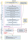 |
Fig. 2. Overview of our approach, which consists of two stages. In the first stage we built a GRG sample, and in the second stage we inferred the properties of the intrinsic GRG population using a forward model. The brackets indicate the different parts of our approach and mention the sections containing the corresponding details. |
4.1. Detecting radio emission
We started out with the publicly available calibrated LoTSS DR2 Stokes I images (Shimwell et al. 2022). For each of the 841 pointings, we ran the PyBDSF radio blob detection software (Mohan & Rafferty 2015) using the same parameters as used in LoTSS DR2 (Shimwell et al. 2022) – notably, this means that we used a 5σ detection threshold. Appendix C provides the full list of PyBDSF parameters and their values.
The output we generated consists of a list of radio blobs with their location and properties. PyBDSF can decompose each radio blob it detects, into one or more 2D Gaussians. For each radio blob, we also saved the corresponding list of Gaussians. These Gaussians function as a source model for each radio blob and will be used in later steps in the ML pipeline 11.
4.2. Calculating radio-to-optical/infrared likelihood ratios
For radio sources, the location of the host galaxy on the sky is close to the flux density–weighted centre of the radio source 12, 13. The likelihood ratio method, which exploits this idea, quantifies the likelihood that a source in one observing band is the correct counterpart to a source in another observing band (e.g. Richter 1975; de Ruiter et al. 1977; Sutherland & Saunders 1992). Williams et al. (2019) used this method to cross-match the unresolved – and some resolved – radio sources of LoTSS DR1 to a combined catalogue of infrared and optical sources. More specifically, the infrared sources came from AllWISE (Cutri et al. 2021), whilst the optical sources came from the Panoramic Survey Telescope and Rapid Response System 1 (Pan-STARRS1; Chambers et al. 2016) DR1 3π steradian survey. The likelihood ratio function that Williams et al. (2019) used is a function of the angular distance between the flux density–weighted centre of the radio source and the flux density–weighted centre of the optical or infrared source, the magnitude of the optical or infrared source, and the colour of the optical or infrared source. The likelihood ratio function also takes into account uncertainties in each of these three dependencies.
We adopted the same procedure as detailed by Williams et al. (2019) to cross-match our simple radio sources (where “simple” is to be understood as in Sect. 4.3) to a combined catalogue of infrared and optical sources. The infrared sources came from unWISE (Schlafly et al. 2019), and the optical sources were now taken from the DESI Legacy Imaging Surveys DR9 (Dey et al. 2019), which boasts deeper imagery than Pan-STARRS1 DR1 used for LoTSS DR1. The unWISE (Schlafly et al. 2019) and DESI Legacy Imaging Surveys DR9 source catalogues are used for LoTSS DR2 cross-matching more generally (Hardcastle et al. 2023). Per pointing, we applied the likelihood ratio method to the full list of radio blobs and to the full list of Gaussians. For both the blobs and the Gaussians, we stored the identifier of the optical or infrared source that produced the highest likelihood ratio, alongside this highest likelihood ratio itself.
4.3. Sorting radio emission with a gradient-boosting classifier
Most radio sources that consist of a single radio blob (mostly unresolved or barely resolved radio sources) can be cross-matched using the likelihood ratio method. However, some resolved radio sources, and certainly most resolved giants (Sect. 2.7), consist of multiple radio blobs as parametrised by PyBDSF, and therefore require radio blob association and cannot be cross-matched using the likelihood ratio alone. To separate the simple from the complex radio blobs in LoTSS DR1, a considerable amount of visual inspection was applied (Williams et al. 2019). For LoTSS DR2, Alegre et al. (2022) trained a gradient-boosting classifier (GBC; Breiman 1997; Friedman 2001) to classify radio blobs as either “simple” or “complex” based on the properties of the radio blobs, the properties of the Gaussians fitted to these blobs, the likelihood ratios for each, and the distance to and properties of the nearest neighbours.
We adopted the procedure of Alegre et al. (2022) and use their trained GBC to separate the simple radio blobs from those that require radio component association beyond PyBDSF’s capabilities and/or optical host identification beyond the scope of the likelihood ratio method of Sutherland & Saunders (1992). We expect most giants to fall in the latter case.
4.4. Associating radio emission into radio sources
We proceeded with automatic radio source component association for the complex radio blobs. Following the procedure laid out by Mostert et al. (2022), for each of these radio blobs, we created a 300″ × 300″ LoTSS DR2 image cutout centred on the radio blob. Next, a fast region-based convolutional neural network (Fast R-CNN; Girshick 2015), adapted and trained for this purpose by Mostert et al. (2022), was applied to these cutouts to predict which (if any) other radio blobs – whether they be complex or simple – form a single physical structure with the central radio blob. For example, the two lobes of an RG, each represented by a radio blob, might be associated together to form a single physical radio source. Due to the fixed 300″ × 300″ image size for which the Fast R-CNN was trained, we expect most radio sources that are associated in our pipeline to have an angular length ϕ < 424″ 14.
The result is a radio source catalogue in which some of the radio blobs have been merged, and a component catalogue that lists for each radio blob to which radio source it belongs. The radio and the component catalogue were completed by appending to them the remaining list of simple radio blobs.
4.5. Identifying host galaxies in the optical and infrared
Barkus et al. (2022) created a method for identifying the optical or infrared host of an extended radio source. The method described by Barkus et al. (2022) takes the radio morphology into account by drawing a ridgeline along the regions of high flux density. The method continues with the application of the likelihood ratio method to quantify which pairs of host galaxy candidates and radio sources are a plausible match. The likelihood ratio LR used in this context follows Eq. (1) of Sutherland & Saunders (1992), with the slight simplification of having the latter’s dependence on two angular offsets replaced by a dependence on a radial angular offset only:
 (32)
(32)
where q(m, c) is a prior on the magnitude m and colour c of the optical host, f(r) is a function of the angular offset between the optical centroid and the radio centroid, and n(m, c) normalises for the number density of optical sources with a certain magnitude m and colour c in the catalogue used for the cross-matching.
To adapt the likelihood ratio for use in the case of extended radio sources, Barkus et al. (2022) implemented the different components of the ratio as follows. For n(m, c), Barkus et al. (2022) estimated the probability density over m and c for a distribution of 50 000 randomly sampled sources from a combined Pan-STARRS–AllWISE catalogue in the region of the sky that overlapped with LoTSS DR1. For q(m, c), they estimated the probability over m and c for sources from the combined Pan-STARRS–AllWISE catalogue that were manually selected to be the most likely optical/near-infrared host for a sample of 950 radio sources with angular length ϕ > 15″. For both n(m, c) and q(m, c), the AllWISE W1 magnitudes were used for m, the Pan-STARRS i-band magnitudes minus the AllWISE W1 magnitudes were used for colour c, and the PDF was formed using a 2D kernel density estimator (KDE; e.g. Pedregosa et al. 2011) with a Gaussian kernel and a bandwidth of 0.2. For extended asymmetric or bent radio galaxies, the optical host is not likely to be found at the radio centroid. Therefore, Barkus et al. (2022) proposed that f(r) should be a function of both the distance between the radio centroid and the optical source ropt, centroid and the smallest distance between the optical source and a ridgeline fitted to the radio source ropt, ridge. Specifically,
 (33)
(33)
with
 (34)
(34)
and
 (35)
(35)
where σr2 = σopt2 + σradio2 + σastr2. We fixed the astrometric uncertainty σastr = 0.2″. The optical position uncertainties σopt are taken from the optical catalogue (generally ∼0.1″), the radio position uncertainty σradio is fixed to 3″, and the uncertainty in the centroid position σc is empirically estimated at 0.2 times the length of the considered radio source. For the 30 optical sources closest to the radio ridgeline, Barkus et al. (2022) calculated the LR and considered the source with the highest LR to be the most likely host galaxy.
We used the method of Barkus et al. (2022) but made three minor adaptations. First, we introduce explicit regularisation for q(m, c) and n(m, c). As the PDF estimates for q(m, c) and n(m, c) are 2D KDEs over sampled (m, c)-distributions, the parts of the (m, c)–parameter space that are sparsely sampled can lead to probabilities that are effectively zero when the realistic theoretical probability should be small but non-zero. Through the q/n-fraction in Eq. (32), the resulting values of LR in the sparsely sampled parts of the (m, c)–parameter space blow up to unrealistic large values or collapse to almost 0 (see Fig. D.1). In practice, these unsampled parts of parameter space are almost never visited by new sources for which we calculate LR. Even so, we add a constant factor to the KDE estimate of q and n to get more robust LR values (see Fig. D.2) and to express the model uncertainties in our functions of q and n. Using 10-fold cross-validation, we empirically select the bandwidths for the KDEs leading to q and n to be 0.4. Second, we propose an alternate form of f(r). For giants, f(r) is rarely dominated by errors in the position of the optical source or that of the radio source. As ropt, centroid and ropt, ridge are slightly correlated, multiplication of fridge(ropt, ridge) and fcentroid(ropt, centroid) under-estimates the chance of low values of ropt, centroid or ropt, ridge. Therefore, we combine ropt, centroid and ropt, ridge into a single parameter rmean that is the mean of the two distance parameters. Furthermore, we observe that the empirical distributions of ropt, centroid, ropt, ridge and rmean for a sample of radio sources with angular length > 1′ Aradio, opt for which optical counterparts were determined via visual inspection do not follow a normal distribution as assumed by Barkus et al. (2022) but rather a lognormal distribution (see Fig. D.3). Instead of estimating the values of the different error components (astrometric error, error in optical position, error in radio position) we use the empirical values of the distribution of f(r) for the sources in Aradio, opt; see Appendix D for details. Third, we replaced the Pan-STARRS1 DR1 catalogue (from which colour c was derived) with the DESI Legacy Imaging Surveys DR9 catalogue, as the latter goes up to an i-band magnitude of 24.
We applied the modified ridgeline method to all radio sources in our pipeline catalogue with angular lengths larger than 1′ and brighter than 10 mJy. We limit the ridgeline procedure to these sources to save time, as the procedure takes multiple seconds per radio source.
After detecting the host galaxies of our radio sources, we checked for spectroscopic redshifts from SDSS (VizieR catalogue V/147/sdss12; Ahn et al. 2012), or if not available, for photometric redshifts from DESI (VizieR catalogue VII/292; Duncan 2022). The SDSS catalogue also provides velocity dispersions and a quasar flag. The DESI catalogue includes a flag (FCLEAN) that indicates whether the optical source used in photometric redshift estimation is free from blending and image artefacts. The catalogue also includes a column (PSTAR) that estimates how likely it is that the optical source is a star based on its colours. In both the ML pipeline and RGZ catalogues, we only retained sources for which FCLEAN = 1 and PSTAR ≤ 0.2.
4.6. Reassessing angular source lengths
Next, we proceeded to reassess the angular source lengths, for both the radio catalogue created using the ML pipeline and the Composite_Size column reported by the RGZ catalogue described by Hardcastle et al. (2023). The angular source lengths in the ML catalogue and the Composite_Size column in the RGZ catalogue are the full width at half maximum (FWHM) of the combined Gaussian components that make up a source, if the source is only composed of a single radio blob. If the radio source is composed of multiple radio blobs, the reported size is the distance between the two furthest removed points on a convex hull that encloses the FWHMs of the blobs that make up the radio source. However, in the literature, the length of a GRG is often reported to be the maximum distance between the signal of a radio source that exceeds three times the image noise σ.
To get the 3σ angular lengths, we applied five steps to all sources in both catalogues with a reported angular length ϕ > 1′. First, we created a square image cutout with a width and height equal to 1.5 times the old angular source length. Second, we mask all neighbouring radio emission. Third, we mask all emission outside an ellipse with a major axis that is the old source length, and a minor axis that is 1.1 times the old source width or a quarter of the old source length if that value is bigger. These numbers are a result of the observation that, with respect to the 3σ angular lengths, the old lengths were almost always significantly overestimated, while the source width tended to be underestimated. Fourth, we mask all remaining emission that is below three times the local noise. Fifth, we fitted a convex hull around the remaining emission and determined the distance between the points on this convex hull that were farthest apart. See Fig. 3 for an illustrative example.
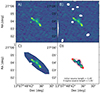 |
Fig. 3. Summary of the angular length re-evaluation for radio source ILTJ130738.79+270355.1. Panels A–D show the initial cutout, the removal of neighbouring sources, the masking of emission outside a convex hull based on the old angular length, and the emission that is left after masking all emission below thrice the local noise σ. The red line segments delineate the convex hull of the left-over emission, and the red points indicate the furthest removed points in this convex hull. The great-circle distance between these points is the 3σ angular length. |
The entire process from source detection (Sect. 4.1) to source list with optical identifications and updated angular lengths (this subsection) took roughly half an hour to one hour per LoTSS DR2 pointing, depending on the detected number of sources. Each pointing can be processed independently, which allowed us to spread the processing of all 841 LoTSS DR2 pointings over 5 nodes of a heterogeneous computer cluster with 80 physical CPU cores in total for three to four days.
Finally, for both the ML pipeline and RGZ catalogues, we calculate the projected proper lengths using the 3σ angular lengths and the redshift estimates corresponding to each source, and discard all sources that do not meet the lp ≥ lp, GRG criterion. For the ML pipeline catalogue, we discarded all internally duplicate GRG candidates using a 1′ cone search. The RGZ catalogue did not contain any internal duplicates. That left us with 7001 GRG candidates in the ML pipeline catalogue and 7044 GRG candidates in the RGZ catalogue.
4.7. Inspecting GRG candidates visually
The following step we took in the creation of our GRG sample was a manual visual inspection of all our GRG candidates. For the RGZ GRG candidates, as described by Hardcastle et al. (2023), at least five different volunteers already inspected the radio and corresponding optical emission, and in most cases the candidates identified in this way were reinspected by a professional astronomer. The purpose of our manual visual inspection was therefore to exclude only those sources where either the radio component association or the host identification was obviously incorrect. For each GRG candidate, a single expert looked at a panel showing the candidate with its neighbouring sources masked and most neighbouring emission masked (akin to panel C in Fig. 3) and a panel showing the candidate in its wider context (akin to panel A in Fig. 3); additionally, the location of the optical host was indicated. We sorted the candidates into three categories: candidates that looked reasonable, candidates that clearly missed (or included too many) significant radio components, and candidates that showed a very unlikely host galaxy location. For the ML pipeline GRG candidates, we initially followed the same procedure as for the RGZ GRG candidates. To speed up the visual inspection, we skipped the 4272 ML pipeline GRG candidates that were verified RGZ giants. After inspecting the ML pipeline GRG candidates once, we subjected all that were not rejected to a second round of visual inspection. The second round was aided by inspecting LoTSS DR2 radio contours over a Legacy Survey DR9 (g, r, z) image cube, where sources from the combined optical–infrared catalogue within the field of view were highlighted.
For the RGZ catalogue, we judged 6550 (93%) GRG candidates to be without issues, 389 (6%) to have radio component issues, and 105 (1%) to have been assigned an unlikely host galaxy. For the 5864 (unique) ML pipeline GRG candidates, we judged 2722 (47%) candidates to be without issues, 1963 (33%) to have radio component issues, and 1179 (20%) to have been assigned an unlikely host galaxy. Radio component association issues for the ML-identified candidates occur because the association method leverages an object detection neural network with rectangular bounding boxes to capture the radio components (Mostert et al. 2022). The large extent of these sources causes many unrelated (fore- and background) radio sources to appear in the rectangular bounding box that encompasses the candidate, increasing the likelihood of erroneous component associations. Future ML radio association methods should consider using instance segmentation instead of object detection with a rectangular bounding box 15. Of the 6550 RGZ giants, 5576 do not appear in previous literature and are thus new discoveries. Of the 2722 ML pipeline giants that are not RGZ giants, 2566 are new discoveries.
Qualitatively, from the visual inspection, we noticed that the verified ML pipeline GRG sample contained more symmetric giants with colinear jets, while the verified RGZ GRG sample contained more giants with complex, bent structures indicative of interaction with the IGM. The ML pipeline did also detect giants with complex structures, but was often unable to fully separate them from all neighbouring unrelated emission. An in-depth comparison between the ML pipeline and RGZ GRG samples is beyond the scope of this work. Figures 4 and 5 each show six examples of previously unknown giants found through our ML-based approach. Through cutouts covering 3′×3′, Fig. 4 shows angularly compact giants; through cutouts covering 6′×6′, Fig. 5 shows more angularly extended specimina.
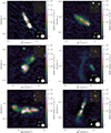 |
Fig. 4. LoTSS DR2 cutouts at central observing frequency νobs = 144 MHz and resolution θFWHM = 6″, centred around the hosts of newly discovered giants. Each cutout covers a solid angle of 3′×3′. Contours signify 3, 5, and 10 sigma-clipped standard deviations above the sigma-clipped median. For scale, we show the stellar Milky Way disk (with a diameter of 50 kpc) generated using the Ringermacher & Mead (2009) formula, alongside a 3 times inflated version. Each DESI Legacy Imaging Surveys DR9 (g, r, z) inset shows the central 1′×1′ square region. As all giants obey ϕ ≥ 1.3′, they must – if not oriented along one of the square’s diagonals – necessarily protrude from this region. Rowwise from left to right, from top to bottom, these giants are ILTJ000212.45+222116.2, ILTJ001115.77+220316.6, ILTJ001350.25+324530.8, ILTJ001831.84+322247.7, ILTJ003025.90+334729.2, and ILTJ003534.45+221937.8. |
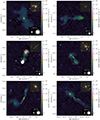 |
Fig. 5. LoTSS DR2 cutouts at central observing frequency νobs = 144 MHz and resolution θFWHM = 6″, centred around the hosts of newly discovered giants. Each cutout covers a solid angle of 6′×6′. Contours signify 3, 5, and 10 sigma-clipped standard deviations above the sigma-clipped median. For scale, we show the stellar Milky Way disk (with a diameter of 50 kpc) generated using the Ringermacher & Mead (2009) formula, alongside a 3 times inflated version. Each DESI Legacy Imaging Surveys DR9 (g, r, z) inset shows the central 1′×1′ square region. As all giants obey ϕ ≥ 1.3′, they must – if not oriented along one of the square’s diagonals – necessarily protrude from this region. Rowwise from left to right, from top to bottom, these giants are ILTJ002943.72+295700.3, ILTJ003010.58+170948.6, ILTJ003521.87+233625.9, ILTJ003712.91+284436.8, ILTJ004002.30+252550.9, and ILTJ235802.49+331838.5. |
4.8. Merging RGZ, ML pipeline, and literature samples
To complete our GRG sample, we iteratively added giants from the literature, going from the newest to the oldest publication. This approach follows from the assumption that newer publications are generally based on more sensitive and higher-resolution observations, leading to more accurate angular length measurements. In an effort to avoid having duplicate giants in the final sample, we only added giants when their host galaxies were more than 10″ away from all host galaxies of already aggregated giants.
The joint RGZ–ML pipeline sample contains 9222 giants. We added 1442 out of the 2193 giants presented by Oei et al. (2023a), 1 out of the 1 giant presented by Oei et al. (2024b) 39 out of the 69 giants presented by Simonte et al. (2022), 62 out of the 62 giants presented by Gürkan et al. (2022), 155 out of the 263 giants presented by Mahato et al. (2022), 178 out of the 174 giants presented by Andernach et al. (2021), 0 out of the 1 giants presented by Masini et al. (2021), 2 out of the 2 giants presented by Delhaize et al. (2021), 0 out of the 2 giants presented by Bassani et al. (2021), 1 out of the 4 giants presented by Tang et al. (2020), 387 out of the 694 giants presented by Dabhade et al. (2020b), and 0 out of the 6 giants presented by Ishwara-Chandra et al. (2020). These additions result in a final catalogue with 11 485 unique giants. This is the first catalogue of giants to contain more than 104 specimina.
Figure 6 shows a Mollweide view of the sky with the locations of both the newly confirmed giants and the giants from the literature. Almost all known giants stay clear of the Galactic Plane, where radio emission from the Milky Way – of which we show the specific intensity function at νobs = 150 MHz in greyscale (Zheng et al. 2017) – makes calibration and imaging harder. In addition, optical host identification is much harder near the Galactic Plane. The default field of view set-up of both our ML pipeline (Sect. 4.4) and of RGZ favours the discovery of giants with angular lengths of a few arcminutes at most. By contrast, the GRG search campaign of Oei et al. (2023a) featured a “fuzzy” ∼5′ lower threshold to allow for an exhaustive manual search with an interactive and dynamic field of view (using Aladin; Bonnarel et al. 2000). Figure 7 demonstrates that these design choices lead to GRG samples with markedly different angular length distributions.
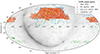 |
Fig. 6. With 11 485 unique giants, we present the largest catalogue of large-scale galactic feedback to the Cosmic Web. The RGZ (orange) and ML pipeline (red) samples are strictly confined to the LoTSS DR2 area, while the sample by Oei et al. (2023a) extends to yet-to-be-released LoTSS pointings processed with the DR2 pipeline. |
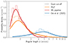 |
Fig. 7. Observed distributions of angular length ϕ, showing that our three LoTSS DR2 search methods target different ranges of ϕ. The largest angular lengths detected by Oei et al. (2023a), RGZ, and the ML pipeline are 132′, 43′, and 8′ respectively, but we limit the horizontal axis to 12′ for interpretability. The vertical line marks the minimum angular length that giants can attain: ϕGRG(lp, GRG = 0.7 Mpc) = 1.3′. |
As a result, the samples complement each other: the sample of Oei et al. (2023a) is more complete at lower redshifts and higher projected lengths, while the RGZ and ML pipeline samples are more complete at higher redshifts and lower projected lengths. Figure 8 demonstrates this point, while Table 1 presents the corresponding statistics of the GRG samples.
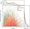 |
Fig. 8. Our sample of RGZ giants (orange squares) and ML pipeline giants (red squares) effectively complements the sample of giants with large angular lengths (blue dots) from the manual search of Oei et al. (2023a). The remaining giants (green pluses) are from earlier literature, as specified in Sect. 4.8. |
Statistics of the GRG samples that we discovered, confirmed, or aggregated.
For comparison of the 3σ lengths of the ML pipeline and RGZ giants to those in other surveys, we inform the reader that the central frequency and the average surface brightness threshold of the observations that we use are νobs = 144 MHz and bν, th = 25 Jy deg−2 respectively.
4.9. Estimating Bayesian model parameters
After having refined our statistical GRG framework (Sect. 2), and after having assembled the largest sample of giants yet (Sects. 4.1–4.8), we combined both advances to perform inference of the length distribution, number density, and lobe volume-filling fraction of giants.
Given that our goal has been to infer properties of the full population of giants, rather than just of those currently observed, we included two main selection effects in our forward modelling. As detailed in Sect. 2.4.1, we parametrised surface brightness selection with three parameters, which are free parameters of the model. As detailed in Sect. 2.4.2, a second cause of selection is the imperfect operation of our three LoTSS DR2 search methods, all of which fail to identify a significant fraction of giants with lobe surface brightnesses above the survey noise level. We modelled this identification selection pobs, ID with a set of logistic functions, regressed to GRG data. We now provide details of this process.
4.9.1. Identification probability functions
To estimate pobs, ID(lp, z) from data, we first selected all giants detected by the joint efforts of our machine learning pipeline, RGZ, and the manual, visual search of Oei et al. (2023a). Next, we retained only those giants that are located in regions of the sky that have been scanned by all three searches. This overlap region in principle corresponds to the full LoTSS DR2 coverage – were it not for the fact that the search of Oei et al. (2023a) skipped over the LoTSS DR1, which had already been scanned by Dabhade et al. (2020b). Therefore, the actual overlap region amounts to the LoTSS DR2 coverage with a spherical quadrangle removed, whose minimum and maximum right ascensions are αmin = 160° and αmax = 230° and whose minimum and maximum declinations are δmin = 45° and δmax = 56°. Appendix E provides an explicit decomposition of our assumed LoTSS DR2 coverage – and therefore implicitly of the overlap region – in terms of disjoint spherical quadrangles.
Some of the retained giants have been detected only in the combined RGZ–ML search, others have been detected only in the Oei et al. (2023a) search, and yet others have been detected in both. We note that, had it operated flawlessly, the combined RGZ–ML search would have detected all sources claimed by Oei et al. (2023a, or at least those that are genuine giants – which should be the vast majority). Therefore, by mapping the (in)ability of the RGZ–ML search to detect the giants of Oei et al. (2023a) as a function of lp and z, one can estimate the RGZ–ML search’s identification probability function, pobs, ID, 1(lp, z). More precisely, for each giant detected by Oei et al. (2023a), we evaluated whether it was also detected in the RGZ–ML search, and stored a corresponding Boolean (that is to say, either 1 or 0). We show these Booleans, at the (lp, z) coordinates of the giants they belong to, as yellow (representing 1) and blue (representing 0) dots in the top-left panel of Fig. 9. Viewing the Boolean at (lp, z) as a realisation of a Bernoulli RV with success probability p = pobs, ID, 1(lp, z), we recognise the inference of the identification probability function as a binary logistic regression problem with two explanatory variables. The background of Fig. 9’s top-left panel shows the corresponding best fit.
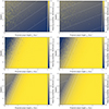 |
Fig. 9. Overview of our determination of the probability to identify giants in the LoTSS DR2 with above-noise surface brightnesses, as a function of projected length and redshift – through Radio Galaxy Zoo: LOFAR and our machine learning pipeline (top row), through the search of Oei et al. (2023a, middle row), and through these methods in unison (bottom row). Each of the upper four panels shows a binary logistic regression following the theory of Sect. 2.4.2 and the practical considerations of Sect. 4.9.1. The left column shows results from all available data, whilst the right column shows results from rebalanced data. In our Bayesian inference, we used the latter results. |
By symmetry, this approach can be reversed to estimate the Oei et al. (2023a) search’s identification probability function, pobs, ID, 2(lp, z). Therefore, for each giant detected in the RGZ–ML search, we evaluated whether it was also detected by Oei et al. (2023a), and stored a corresponding Boolean. In the same way as before, we show these Booleans in the middle-left panel of Fig. 9. The panel’s background shows the best logistic fit.
We combine the two identification probability functions, pobs, ID, 1(lp, z) and pobs, ID, 2(lp, z), in point-wise fashion as to obtain a single function pobs, ID(lp, z). To do so, we follow the minimal combination rule of Eq. (19).
We remark that, by giving each Boolean in these logistic regressions an equal weight, the resulting functions are tuned to fit crowded regions of projected length–redshift parameter space best – at the expense of accuracy in sparser regions. To increase the accuracy of the functions for the parameter space at large, we performed a simple rebalancing step. First, we calculated the mean number density in the parameter space given by lp ∈ [0.7, 5 Mpc]×[0, 0.5]∋z. We then selectively subsampled the data in crowded regions, following the rule that the number density in each bin of width 0.5 Mpc and height 0.05 should not exceed twice the mean number density of the entire parameter space. We show the rebalanced data, alongside refitted logistic models, in the right column of Fig. 9. We report the rebalanced model coefficients in Table 2, and treat them as constants during the Bayesian inference.
4.9.2. Inference in practice
In this work, we constrained the parameters of Sect. 2’s GRG population model via a projected length–redshift histogram. From our most extensive sample of giants, we selected those with 0.7 Mpc = :lp, GRG < lp < 5.1 Mpc and 0 < z < zmax := 0.5 that lie in the LoTSS DR2 coverage as specified in Appendix E. We did not include the giants from Oei et al. (2023a) for which only a lower bound to the redshift is known. This selection retained 2685 out of 11 485 giants. We used these giants to fill a histogram with bins of width Δlp = 0.1 Mpc and Δz = 0.02. We did not systematically explore the effect of these bin size parameters on the resulting inference. However, the smaller one chooses the bins, the higher the numerical cost will be. On the other hand, if the bins are chosen much larger than the typical scales over which the underlying observed projected length–redshift distribution 16 varies, then some ability to extract parameter constraints will be lost.
To compute the posterior distribution over the six parameters θ = [ξ(lp, GRG),Δξ, bν, ref, σref, ζ, nGRG], we assumed a uniform prior and brute-force evaluated the likelihood function over a regular grid that covers a total of 2.1 × 10⁹ parameter combinations17. In doing so, we applied the Poissonian likelihood trick described in Appendix B, which sped up our computations by one to two orders of magnitude. Table 2 provides the parameter ranges for which we evaluated the likelihood (which coincide with their prior distribution ranges), alongside all of the model’s constants and their assumed values. Because each likelihood function evaluation can be computed independently of the others, the problem is fully parallelisable. In practice, we distributed the ∼104 core-hours Python calculation over ∼1500 virtual cores, which were spread across ∼20 nodes of a computer cluster. Next, we generated samples from the posterior distribution using rejection sampling (e.g. Rice 2006). We subsequently used these samples to calculate probability distributions for derived quantities18.
5. Results
By combining an unparalleled sample of giant radio galaxies with a rigorous forward model, we have produced a posterior distribution over parameters that characterise the intrinsic population of giants. Figure 10 summarises the posterior over parameter hexads θ = [ξ(lp, GRG),Δξ, bν, ref, σref, ζ, nGRG] by means of its one- and two-dimensional marginal distributions. In this section, we analyse our newfound parameter constraints.
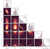 |
Fig. 10. Likelihood function over θ = [ξ(lp, GRG),Δξ, bν, ref, σref, ζ, nGRG], based on 2685 projected lengths and redshifts of giants up to zmax = 0.5. We show all two-parameter marginals of the likelihood function, with contours enclosing 50% and 90% of total probability. We mark the maximum likelihood estimate (MLE) values (grey dot) and the likelihood mean values (grey cross). The one-parameter marginals again show the MLE (dash-dotted line), a mean-centred interval of standard deviation–sized half-width (hashed region), and a median-centred 90% credible interval (shaded region). |
5.1. Length distribution of giant radio galaxies
Radio galaxies enrich the IGM with magnetic fields, but giants – given their megaparsec-scale reach – appear uniquely capable of seeding the more remote regions of the Cosmic Web. Consequently, scientific interest in quantifying the length distribution of giants has arisen from the possibility that giants contribute significantly to cosmic magnetogenesis. The question at hand is deceivingly simple: how common are giants of various lengths?
As pointed out by Oei et al. (2023a), due to selection effects, the observed projected length distribution is not a reliable estimate of the true projected length distribution. Worse still, the relevant selection effects might not be quantitatively known a priori, requiring joint inference of the length distribution, and the selection effect parameters. Oei et al. (2023a) performed such a joint inference, and found that their data were consistent with an underlying population of giants with Pareto-distributed lengths, characterised by tail index ξ = −3.4 ± 0.5. In the current work, we have relaxed the assumption of perfect Paretianity, and explore whether the data are consistent with a curved power law PDF for the GRG projected proper length RV Lp | Lp ≥ lp, GRG. The marginals of Fig. 10 suggest that they are – in fact, the data strongly favour curvature, with a tail index at lp, 1 := lp, GRG := 0.7 Mpc of ξ(lp, GRG) = − 2.8 ± 0.2 and a total increase in tail index up to lp, 2 := 5 Mpc of Δξ = −2.4 ± 0.3. Given the small relative uncertainty on the latter value, our data appear inconsistent with perfect Paretianity (Δξ = 0). We note that our notion of “data” is different from that in Oei et al. (2023a): not only do we use more than a thousand additional giants, we also make more effective use of their redshift information. For further discussion, see Sect. 6.2.
It remains an open question whether giants can be understood as part of the ordinary radio galaxy population, or whether they evolve through qualitatively different physical processes. As pointed out in Sect. 4.1.5 of Oei et al. (2023a), a curved power law PDF for Lp | Lp ≥ lp, GRG is consistent with a scenario in which giants share a broader length continuum with smaller radio galaxies. More specifically, if the broader radio galaxy length distribution is approximately lognormal, as appears justifiable on statistical grounds, then ξ should decrease throughout the distribution’s right tail – that is, throughout the GRG range. Future research should determine whether such a unified non-giant RG–GRG scenario is also quantitatively consistent with the decrease in ξ we have inferred here. In addition, our inferences of ξ(lp, GRG) and Δξ are important in constraining Sect. 5.3’s GRG lobe volume-filling fraction.
5.2. Number density of giant radio galaxies
The extent to which giants have contributed to cosmic magnetogenesis depends on their intrinsic number density – which need not necessarily be a constant, but could have evolved over time. Observationally, giants are considered rare in comparison to smaller radio galaxies. However, because giants are presumably strongly affected by surface brightness selection, this present-day observed rarity might not translate to an intrinsic rarity. Excitingly, by forward modelling selection effects – and in particular surface brightness selection – we can constrain the intrinsic comoving GRG number density between z = 0 and z = zmax, which we denote simply by nGRG.
The bottom-right one-dimensional marginal of Fig. 10 shows a strongly skewed distribution for nGRG, with a marginal mean 𝔼[nGRG] = 13 ± 10 (100 Mpc)−3 and a 95% probability that nGRG > 4 (100 Mpc)−3. These number densities are a factor of order unity higher than those of Oei et al. (2023a), who inferred a marginal mean 𝔼[nGRG] = 4.6 ± 2.4 (100 Mpc)−3 and a 90% probability that nGRG < 6.7 (100 Mpc)−3.
The joint marginal distribution of nGRG and bν, ref reveals a strong inverse relationship, whose origin is easy to grasp. Models in which giants are relatively rare (i.e. with low nGRG) but with relatively mild surface brightness selection (i.e. with high bν, ref) are about as successful in reproducing the data-derived projected length–redshift histogram as models in which giants are relatively common (i.e. with high nGRG) but with relatively severe surface brightness selection (i.e. with low bν, ref). The narrowness of the joint distribution also suggests that, if estimates of bν, ref would reveal it to be ≳10 Jy deg−2, it should be possible to break the degeneracy and accurately determine nGRG.
Recent work (Oei et al. 2024a) suggests that the comoving number density of luminous, non-giant radio galaxies (LNGRGs), understood to have radio luminosities at 150 MHz of lν ≥ 1024 W Hz−1 and projected lengths lp < lp, GRG := 0.7 Mpc, is nLNGRG = 12 ± 1 (100 Mpc)−3. Our work suggests that giants might be comparably common. If this is indeed the case, then the widespread belief that giants form a rare population of radio galaxies must be revised.
5.3. Lobe volume-filling fraction of giant radio galaxies
The present-day volume-filling fraction of the lobes of giants in clusters and filaments of the Cosmic Web, 𝒱GRG − CW(z = 0), is not a parameter of our model, but rather a derived quantity. As briefly discussed in Sect. 4.9.2, we compute its probability distribution using the parameter hexads that we have obtained by rejection sampling from the posterior. For each sampled hexad, we compute ξ(lp) using ξ(lp, GRG), Δξ, and Eq. (8), then fLp | Lp ≥ lp, GRG(lp) using Eq. (9), and finally 𝒱GRG − CW(z = 0) using nGRG and Eq. (26).
To arrive at Eq. (26), we assumed in Eq. (24) that RG projected proper lengths and two-lobe proper volumes obey a power law relation with scatter. To investigate the validity of this assumption, we collected the projected proper lengths and two-lobe proper volumes of all Fanaroff–Riley II RGs in the “representative” sample of Ineson et al. (2017)19. Among these RGs are just seven giants. To more reliably probe the projected proper length–two-lobe proper volume relation for giants, we supplemented this sample with the giant of NGC 6185, the longest spiral galaxy–generated RG known (Oei et al. 2023b), and with Alcyoneus, the longest elliptical galaxy–generated RG known (Oei et al. 2022). Oei et al. (2023b) estimated that the giant of NGC 6185 measures lp = 2.45 ± 0.01 Mpc and has a two-lobe proper volume V = 0.35 ± 0.03 Mpc3. Similarly, Oei et al. (2022) estimated that Alcyoneus measures lp = 4.99 ± 0.04 Mpc and has a two-lobe proper volume V = 2.5 ± 0.3 Mpc3. We show the empirical lp − V relation for the resulting sample in Fig. 11. Tentatively, we consider the assumed power law relation between projected proper length and two-lobe proper volume justified, although we warn that the sample size is small and that we have not made corrections for selection effects. Through least-squares minimisation in log–log space, we obtained two best-fit power law relations: one for giants only (green line) and for all RGs (grey line). In order to calculate Eq. (26), we adopted the parameters from the giant-based fit: VGRG = 1.2 × 10⁻² Mpc3 and γ = 2.7.
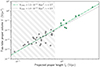 |
Fig. 11. Empirical relation between projected proper length and two-lobe proper volume for RGs from Ineson et al. (2017), Oei et al. (2022, 2023b). The power law–like trend motivates Eq. (24). The green fit is based on giants only, whilst the grey fit is based on all RGs. VGRG is the mean two-lobe proper volume of the shortest possible giants (i.e. giants for which lp = lp, GRG), while γ is the exponent of the power law. For self-similar RG growth, γ = 3. |
For each sampled hexad, we calculate ![Mathematical equation: $ \mathbb{E}[L_{\mathrm{p}}^{\gamma}\ \vert\ L_{\mathrm{p}} \geq l_{\mathrm{p,GRG}}] $](/articles/aa/full_html/2024/11/aa48897-23/aa48897-23-eq39.gif) using the law of the unconscious statistician. The mean two-lobe volume of a giant is 𝔼[V | Lp ≥ lp, GRG](z = 0) = 5.1 ± 0.3 × 10⁻² Mpc3. As in Oei et al. (2023a), we assume that clusters and filaments comprise 5% of the Local Universe’s volume (Forero-Romero et al. 2009): 𝒱CW(z = 0) = 5%. We show the resulting posterior distribution over 𝒱GRG − CW(z = 0) in Fig. 12. This probability distribution inherits its skewness from the skewed marginal of nGRG. We find
using the law of the unconscious statistician. The mean two-lobe volume of a giant is 𝔼[V | Lp ≥ lp, GRG](z = 0) = 5.1 ± 0.3 × 10⁻² Mpc3. As in Oei et al. (2023a), we assume that clusters and filaments comprise 5% of the Local Universe’s volume (Forero-Romero et al. 2009): 𝒱CW(z = 0) = 5%. We show the resulting posterior distribution over 𝒱GRG − CW(z = 0) in Fig. 12. This probability distribution inherits its skewness from the skewed marginal of nGRG. We find  and a posterior mean and standard deviation of 𝒱GRG − CW(z = 0) = 1.4 ± 1.1 × 10⁻⁵. These results appear statistically consistent with that of Oei et al. (2023a):
  .
.
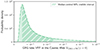 |
Fig. 12. Posterior distribution for the instantaneous, present-day GRG lobe volume-filling fraction in clusters and filaments of the Cosmic Web, 𝒱GRG − CW(z = 0). |
While they appear low at first sight, we speculate that these numbers are consistent with a scenario in which giants contribute significantly to cosmic magnetogenesis. To see why, we first note that the number of giants that have ever existed might exceed those that exist now by two orders of magnitude: giants are actively powered for ∼101 − 103 Myr (e.g. Hardcastle 2018; Gürkan et al. 2022; Oei et al. 2022; Dabhade et al. 2023), the electron ageing time-scale is ≲102 Myr, the Universe is ∼104 Myr old, and one may assume – in the absence of clear evidence to the contrary – that the comoving number density of giants nGRG has remained roughly constant over cosmic time20. Second, a likely large fraction of all giants that existed throughout cosmic history lived when the Universe was significantly smaller. More specifically, all giants at ![Mathematical equation: $ z \geq z_{10} := \sqrt[3]{10}-1 \approx 1.15 $](/articles/aa/full_html/2024/11/aa48897-23/aa48897-23-eq42.gif) lived when the Universe’s volume was at least an order of magnitude smaller; this period covers ∼38% of all cosmic time. If the mean two-lobe proper volume of giants 𝔼[V | Lp ≥ lp, GRG] and the VFF of clusters and filaments 𝒱CW have remained roughly constant over the redshift range [0, z10], then by Eq. (26) we have 𝒱GRG − CW(z = z10) = 10 ⋅ 𝒱GRG − CW(z = 0)21. Third, buoyant lobes might deposit magnetic fields in their wake, while diffusion, turbulence, and merger and accretion shocks from large-scale structure formation might have spread the contents of GRG lobes further through the IGM (e.g. Enßlin 2003). The typical extent of a GRG lobe along a single spatial dimension, ℓ, can be considered to be
lived when the Universe’s volume was at least an order of magnitude smaller; this period covers ∼38% of all cosmic time. If the mean two-lobe proper volume of giants 𝔼[V | Lp ≥ lp, GRG] and the VFF of clusters and filaments 𝒱CW have remained roughly constant over the redshift range [0, z10], then by Eq. (26) we have 𝒱GRG − CW(z = z10) = 10 ⋅ 𝒱GRG − CW(z = 0)21. Third, buoyant lobes might deposit magnetic fields in their wake, while diffusion, turbulence, and merger and accretion shocks from large-scale structure formation might have spread the contents of GRG lobes further through the IGM (e.g. Enßlin 2003). The typical extent of a GRG lobe along a single spatial dimension, ℓ, can be considered to be
}{2}}, \end{aligned} $$](/articles/aa/full_html/2024/11/aa48897-23/aa48897-23-eq43.gif) (36)
(36)
meaning that ℓ(z = 0) = 0.295 ± 0.006 Mpc ∼ 10−1 Mpc. If, after jet fuelling stops, lobes rise buoyantly to the edges of filaments at the speed of sound, their total traversed path length will be ∼100 Mpc (e.g. Gheller & Vazza 2019). The columns through which GRG lobes have risen might therefore have a volume that is an order of magnitude larger than the lobes’ own. Taken together, these three effects could render the present-day VFF of magnetic fields that were once contained in the lobes of giants higher than 𝒱GRG − CW(z = 0) by four (i.e. 2 + 1 + 1) or more orders of magnitude. This, in turn, suggests a significant astrophysical seeding potential. For instance, assuming four orders of magnitude, ∼10% of the volume of today’s Cosmic Web should have been magnetised by giants.
We finally point out that giant-induced IGM magnetic fields could have strengths consistent with observational constraints. At the moment, the lowest magnetic field strengths measured in giant radio galaxy lobes, as inferred from images of Alcyoneus and the giant generated by NGC 6185 assuming the equipartition or minimum energy condition, are 400 − 500 nG (Oei et al. 2022, 2023b). If such field strengths would be typical, and buoyancy and diffusion lowers the density of field lines by an order of magnitude, then the typical giant-induced IGM field strength would be ∼10 nG. This is in agreement with recent radio estimates and limits (e.g. Table 1 of Vazza et al. 2021). We note that this argument ignores possibly significant amplification and decay mechanisms, such as turbulent amplification and decay.
6. Discussion
Below, we discuss how our ML pipeline and GRG population inference compare to earlier work.
6.1. Comparison with previous machine learning search techniques
Proctor (2016) applied an ML approach to search for GRG candidates by looking for likely pairs of (unresolved) radio lobes with the required angular length in the NRAO VLA Sky Survey (NVSS; Condon et al. 1998). For this radio source component association problem, Proctor (2016) trained an oblique classifier (a type of decision tree ensemble; Murthy et al. 1993), using six source finder–derived features on 51 195 pairs of radio components, 48 of which were verified giants. This method proved to be useful under the assumption that giants generally appear as an isolated pair of unresolved radio blobs, which is the case for NVSS with its 45″ resolution and 450 μJy beam−1 sensitivity. Dabhade et al. (2020a) visually inspected the 1600 GRG candidates presented by Proctor (2016) and confirmed 151 giants, which implies a 9% precision for the GRG candidate predictions. However, Proctor (2016) expect that giants with resolved lobes – which rule-based source finders often incorrectly break down into multiple separate sources – require a different approach, and virtually all GRG lobes in LoTSS are resolved22. It works in our favour that the convolutional neural network in our ML pipeline (Sect. 4.4) was specifically designed to use the morphology of the resolved, extended emission as a cue for the radio source component association. Furthermore, as the source suggestions from our ML pipeline include optical host identifications, the candidates that we inspected not only have the required angular length but also have a host galaxy and corresponding redshift estimate assigned. This allows us to visually inspect only those radio sources that fulfil the projected proper length lp, GRG := 0.7 Mpc requirement. Overall, our ML pipeline has a precision of 47% for the GRG candidates that it suggests.
6.2. Comparison with previous inference strategies
Compared to the approach of Oei et al. (2023a), our approach makes better use of the redshift information available for each giant. More specifically, we use the redshifts to make a “redshift-resolved” observed projected length histogram, while Oei et al. (2023a) only compared a “redshift-collapsed” distribution of observed projected lengths to forward model predictions of Lp, obs | Lp, obs ≥ lp, GRG. Effectively, Oei et al. (2023a) therefore used for each giant only Boolean redshift information, 𝕀(zi < zmax): that is, a truth value indicating whether or not the giant with index i resides at a redshift below the maximum considered value.
In addition, our work changed the comoving number density of giants, nGRG, from a derived quantity to a model parameter. This approach acknowledges the fact that the observed number of giants, either for a specific projected length–redshift bin or for the parameter space in its entirety, scales linearly with nGRG (if the selection effects remain the same). Therefore, there is intrinsic population information contained in the observed number of giants. However, by comparing predicted and observed probability distributions only, Oei et al. (2023a) did not exploit this fact.
6.3. Future work
With the advent of large-scale, sensitive, low-frequency sky surveys such as the LoTSS, the Evolutionary Map of the Universe survey (EMU; Norris et al. 2011), and the arrival of next-generation instruments such as the SKA (Dewdney et al. 2009) and the DSA-2000 (e.g. Hallinan et al. 2019; Connor et al. 2022) later this decade, opportunities will arise to detect many more giants than have been found hitherto. It is therefore likely that automated approaches to giant finding and host association will become only more relevant in the future.
Regarding our own machine learning–based pipeline, there is significant room to improve both the radio component association and the host association. Visual inspection indicated a precision of 47% and the empirically determined pobs, ID in Fig. 9 showed that even in combination with the RGZ sample, the ML pipeline recall does not surpass 70%. Sensible paths to improve the radio component association within the ML pipeline architecture include switching from rectangular bounding box–based object detection (the Fast R-CNN used in this article) to pixel-based instance segmentation and using a larger convolutional backbone (e.g. Liu et al. 2022; Wright et al. 2010) or a transformer-based backbone (e.g. Liu et al. 2021; Zhang et al. 2022; Li et al. 2022). Mostert et al. (2022) conclude that a larger convolutional neural network is not effective unless one also significantly increases the quantity of high-quality training data, and in general, transformers require even more training data than convolutional neural networks (e.g. Wang et al. 2022). To that extent, adding a filtered version23 of the available LoTSS DR2 RGZ annotations (Hardcastle et al. 2023) to the training data can be considered. Furthermore, assembling a joined data set encompassing the (labelled) survey data of other low frequency radio telescopes can be considered. Pretraining on this data set can benefit radio galaxy component association, host identification and morphological classification tasks across the board.
Finally, there appear to be clear opportunities to make the population-based forward model presented in Sect. 2 more accurate. For example, at present, we have neglected photometric redshift uncertainties; however, the consequences of these uncertainties appear perfectly possible to forward model. One such currently ignored consequence is Eddington bias: as RGs with projected lengths lp = 0.6 Mpc are intrinsically more common than those with projected lengths lp = 0.8 Mpc, redshift error–induced projected length errors have the net effect of falsely raising the number of supposed giants with projected lengths near lp, GRG := 0.7 Mpc. This effect could contaminate the inference of ξ(lp, GRG). Somewhat more challenging, but plausibly of greater value, would be a further exploration of how surface brightness selection is effectively modelled. A major focus of such an exploration would be to analyse the surface brightness characteristics of hitherto discovered giants. As the masked cutouts of Fig. 3 suggest, the machine learning–based pipeline described in this work offers the exciting potential to amass – fully automatically – surface brightness properties for thousands of giants. The availability of such properties for a large fraction of observed giants also allows one to fit the forward model to an observed projected length–redshift–surface brightness histogram, rather than to an observed projected length–redshift histogram only. It is highly likely that adding another dimension to the data yields tighter parameter constraints. To make the identification probability functions of Fig. 9 more accurate, it appears promising to have an expert visually (and exhaustively, i.e. without imposing angular length thresholds) comb through a small representative region of LoTSS DR2 in search of giants. The resulting data set would provide a better basis for determining the identification probability functions than the RGZ–ML or Oei et al. (2023a) data sets used in this work. We note that the Boötes LOFAR Deep Field search of Simonte et al. (2022) does not appear suited for this purpose, as the increased depth of this field renders it unrepresentative of LoTSS DR2 as a whole. Finally, the model could be expanded in an attempt to measure cosmological evolution of, for example, nGRG. However, we note that adding additional parameters to the model necessitates adopting more efficient inference techniques, such as Markov chain Monte Carlo or nested sampling. The associated numerical gain would, in part, be negated by losing the speed-up associated to the likelihood trick of Appendix B.
To determine the instantaneous VFF of GRG lobes in the Cosmic Web, 𝒱GRG − CW(z), one needs to calculate the mean GRG two-lobe proper volume 𝔼[V | Lp ≥ lp, GRG](z). To estimate the latter quantity, we have proposed to leverage the apparent power law relation between projected length and two-lobe volume shown in Fig. 11. However, the fit in this work is based on data of just nine giants. To improve this situation, we recommend expanding the capabilities and automating the parametric Bayesian lobe volume estimation method introduced by Oei et al. (2022, 2023b). This method could then be applied to thousands of our ML pipeline’s masked cutouts, such as the one in Fig. 3. This effort would increase the number of giants on which our fit of the projected length–two-lobe volume power law is based by two to three orders of magnitude.
7. Conclusions
In this work, we concatenated an existing crowd-sourced radio–optical catalogue, a new ML pipeline to automate radio–optical catalogue creation, and a Bayesian forward model to build a next-generation giant radio galaxy discovery and characterisation machine. Applying this setup to the LOFAR Two-metre Sky Survey, we uncovered thousands of previously unknown giants, confirmed thousands of GRG candidates, and constrained the properties of the underlying population. As not all new sources have received a thorough manual check, we advise users to remain critical when using our catalogue.
-
The LoTSS is an ongoing sensitive, high-resolution, low-frequency radio survey whose second data release (DR2) covers 27% of the northern sky. As the number of detected sources already ranges in the millions, it has become unfeasible (at least for small scientific teams) to conduct manual visual searches for giants, in particular for those with angular lengths close to the lower limit of 1.3′.
-
To address this challenge, we scanned all 841 LoTSS DR2 pointings – which together cover more than 5000 sq. deg of the northern sky – with an ML pipeline that crucially includes the convolutional neural network of Mostert et al. (2022), designed for the association of radio components for highly resolved radio galaxies, and an adapted version of the automated optical host galaxy identification heuristic developed by Barkus et al. (2022). Used as a GRG detection system, our ML pipeline has a precision of 47%, a significant improvement over the 9% precision obtained using the previously best ML GRG detection model (Proctor 2016; Dabhade et al. 2020a). We merged the resulting giant candidate sample with that of the RGZ citizen science campaign (Hardcastle et al. 2023), homogenised the angular lengths, and subjected the candidates to a visual quality check. The result is a sample of more than 8000 newly confirmed giants, of which a large fraction are considered genuine beyond reasonable doubt. More than 104 unique giants have now been identified and published.
-
We expand the population-based statistical forward model of Oei et al. (2023a) designed to constrain the geometric properties of giants. In particular, by modelling the PDF of the radio galaxy projected length RV Lp as a curved power law, we automatically also model the PDF of the giant radio galaxy projected length RV Lp | Lp ≥ lp, GRG as a curved power law. We assume that these projected length distributions do not undergo intrinsic evolution between cosmological redshifts of z = zmax and z = 0, and likewise assume an intrinsically constant comoving GRG number density throughout this redshift range. We model surface brightness selection by assuming a lognormal lobe surface brightness distribution at the survey’s central frequency νobs, which is valid for radio galaxies of intrinsic proper length lref at redshift z = 0. We relate lobe surface brightness distributions for radio galaxies of other lengths and at other redshifts to this reference distribution. In addition, we model selection caused by the imperfect ability of search methods to identify all in-principle identifiable giants. For this purpose, we use logistic functions of projected length lp and redshift z.
-
We then sought to identify all model parameter hexads that can reproduce the projected length–redshift histogram of the joint RGZ–ML–Oei et al. (2023a) LoTSS DR2 GRG sample. Through a simple Poissonian likelihood and a uniform prior distribution, we constructed a posterior distribution over the model parameters. By confronting the model with an observed projected length–redshift histogram, rather than with an observed projected length distribution only (as has been done in Oei et al. 2023a), we obtain tighter parameter constraints.
-
We find evidence in support of the claim that the projected lengths of giant radio galaxies follow a curved power-law PDF, whose tail index is equal to ξ(lp, GRG) = − 2.8 ± 0.2 at lp, 1 = lp, GRG := 0.7 Mpc and increases by Δξ = −2.4 ± 0.3 (i.e. decreases by 2.4 ∓ 0.3) in the projected length interval leading up to lp, 2 = 5 Mpc. The predicted median lobe surface brightness at νobs = 150 MHz, lref = 0.7 Mpc, and z = 0 is equal to bν, ref = 30 ± 20 Jy deg−2. This surface brightness level is lower than previously thought. Tight degeneracies resembling inverse relations exist between bν, ref and the reference surface brightness dispersion measure σref, and between bν, ref and the GRG number density nGRG. The latter relation suggests that giants might be more common than previously thought. At nGRG = 13 ± 10 (100 Mpc)−3, giants appear to be of an abundance comparable to that of luminous non-giant radio galaxies. We conclude that, at any moment in time, a significant fraction of the radio galaxy population is in a GRG phase. As an immediate consequence, the fraction of radio galaxies that end their lives as giants must be even higher.
-
Finally, we generate a posterior distribution for the instantaneous volume-filling fraction of GRG lobes in clusters and filaments of the Cosmic Web, 𝒱GRG − CW(z = 0) – a key statistic required for determining the cosmic magnetogenesis potential of giants. We find 𝒱GRG − CW(z = 0) = 1.4 ± 1.1 × 10⁻⁵. The mean two-lobe proper volume of a giant is 𝔼[V | Lp ≥ lp, GRG](z = 0) = 5.1 ± 0.3 × 10⁻² Mpc3. If a GRG population similar to that in the Local Universe has existed for most of the lifetime of the Universe, and IGM mixing processes are significant, then it appears possible that magnetic fields originating from giants permeate throughout significant (≳10%) fractions of today’s Cosmic Web.
Using modern automation and inference techniques (which still leave significant room for future improvements), we conducted the most detailed study of the abundance and geometrical properties of giants to date. These cosmic colossi may provide a previously underappreciated contribution to astrophysical magnetogenesis.
In Cosmic Web filament environments, where giants appear most common (Oei et al. 2024a), lobes may expand along the Hubble flow, rendering their proper and comoving extents different. To avoid ambiguity, we stress that our projected lengths are proper instead of comoving. A less precise synonym for “projected proper length” often found in the literature is “largest linear size”.
This assumption is admissible, because even if the relative orientations of RGs and filaments are not random (e.g. Beckmann et al. 2024; Codis et al. 2018), the uniformity of filament orientations on large scales leads to uniform RG orientations on large scales.
We have also assumed that lp, GRG > lmin, which is the obvious case to consider.
This is an example of a more general rule: for any RV X,
This line of reasoning implicitly assumes that the distribution of Lp is unimodal.
In a flat Friedmann–Lemaître–Robertson–Walker universe, the dimensionless Hubble parameter E is
 (4)
(4)
In case methods tend to find independent subsets of identifiable giants,
 (12)
(12)
We note that it is possible to design methods that find subsets of identifiable giants that have even less overlap than independent subsets have.
If one includes this term, it only needs to be calculated once. For numerical stability, it is helpful to note that
 (20)
(20)
LoTSS DR2 is publicly available at https://lofar-surveys.org/dr2_release.html
The Zooniverse website is https://zooniverse.org
However, as we discuss in Sect. 4.6 these source models are not always adequate for extended, well-resolved radio sources.
In this context, “close” refers to angular distances comparable to the survey’s resolution.
The flux density–weighted centre of a radio component is the sum of the product of position and flux density for each pixel in the area where PyBDSF found significant emission, divided by the area’s total flux density. This calculation is performed twice: once for determining the right ascension and once for determining the declination of the centroid. The flux density–weighted centre of a multi-component radio source is the flux density–weighted average of the components’ individual flux density–weighted centres.
If predicted associations from neighbouring cutouts have an overlapping radio blob, the associations will be merged. For example: in cutout 1 lobe A and core B are associated and in cutout 2 core B and lobe C are associated, then the set (lobe A, core B, and lobe C) will enter the catalogue as a single radio source, thereby creating the possibility of detecting radio sources with angular length ϕ > 424″.
For the distinction between object detection and instance segmentation, see Lakshmanan et al. (2021).
With the “underlying” observed projected length–redshift distribution, we mean the observed projected length–redshift distribution one would obtain in the limit of an infinite number of observed giants.
This approach is feasible by virtue of the low numerical cost of each likelihood function evaluation. Its main advantage is its simplicity: there are no parameters to tune that govern the method’s convergence behaviour. Once the model is expanded to include more parameters, or when selection effects with higher numerical cost are incorporated, more efficient (though more complicated) methods such as Markov chain Monte Carlo or nested sampling will become necessary.
To calculate probability distributions over quantities that are a function of the parameters, such as the Local Universe GRG lobe VFF, 𝒱GRG − CW(z = 0), or the joint search completeness function C, we could in principle evaluate these quantities for each parameter combination of the aforementioned grid and weigh each grid point’s result by the associated likelihood (or, equivalently, posterior probability). However, some derived quantities are costly to compute, so that excessive evaluations should be avoided.
We calculated projected proper lengths by summing the lobe tip distances of both lobes. For RGs for which Ineson et al. (2017)’s Table 5 reports data on only one lobe, we assumed that the other lobe has an identical lobe tip distance and volume.
The dynamics of RGs are different at early epochs; reasons include a less developed large-scale structure but higher mean cosmic densities, higher AGN cold gas accretion and galaxy merger rates (e.g. O’Leary et al. 2021), and more severe inverse Compton energy losses to the CMB (e.g. Hardcastle 2018). Giants possibly representative of early epochs are discussed in e.g. Mahato et al. (2022).
Based on Millennium simulations, which are dark matter–only, Cautun et al. (2014) suggest that 𝒱CW may instead have decreased from ∼10% at z = z10 to ∼5% at z = 0. This would imply that 𝒱GRG − CW(z = z10) is a factor ∼2 smaller than we claim here.
As all giants have angular lengths ϕ ≥ 1.3′, they cover at least 13 LoTSS 6″ beams. This suggests that a single GRG lobe will cover multiple beams, too.
For example, by identifying a handful of very active and expert volunteers and increasing the weight of their votes.
In two dimensions, the Euclidean distance between the origin and a point whose Cartesian coordinates are independent, zero-mean, and equal-variance normal random variables, is Rayleigh distributed. This motivates modelling the angular distance between the optical counterpart and the radio centroid with a Rayleigh distribution. The appropriate value of the distribution’s parameter likely depends (positively) on the angular length of the RG considered; as such, one would not expect a single Rayleigh distribution to work for all RGs.
Acknowledgments
The full GRG catalogue with host identifications will soon be available on the VizieR catalogue service hosted by the Centre de Données astronomiques de Strasbourg (CDS). M.S.S.L. Oei and R.J. van Weeren acknowledge support from the VIDI research programme with project number 639.042.729, which is financed by the Dutch Research Council (NWO). M.S.S.L. Oei also acknowledges support from the CAS–NWO programme for radio astronomy with project number 629.001.024, which is financed by the NWO. Finally, M.S.S.L. Oei acknowledges support from the ERC Starting Grant ClusterWeb 804208. L. Alegre is grateful for support from the UK STFC via CDT studentship grant ST/P006809/1. M.J. Hardcastle acknowledges support from the UK STFC [ST/V000624/1]. B. Barkus is grateful for support from the UK STFC. We would like to thank Huib Intema for enabling the cross-institute collaboration on the Leiden Observatory computer infrastructure. We would like to thank Frits Sweijen for coding the very useful https://github.com/tikk3r/legacystamps. This research has made use of the Python astropy package (Astropy Collaboration 2018); the VizieR catalogue access tool (Ochsenbein et al. 2000), CDS, Strasbourg, France (DOI: https://doi.org/10.26093/cds/vizier); and the “Aladin Sky Atlas” developed at CDS, Strasbourg Observatory, France (Bonnarel et al. 2000; Boch & Fernique 2014). LOFAR data products were provided by the LOFAR Surveys Key Science project (LSKSP; https://lofar-surveys.org/) and were derived from observations with the International LOFAR Telescope (ILT). LOFAR (van Haarlem et al. 2013) is the Low Frequency Array designed and constructed by ASTRON. It has observing, data processing, and data storage facilities in several countries, which are owned by various parties (each with their own funding sources), and which are collectively operated by the ILT foundation under a joint scientific policy. The efforts of the LSKSP have benefited from funding from the European Research Council, NOVA, NWO, CNRS-INSU, the SURF Co-operative, the UK Science and Technology Funding Council and the Jülich Supercomputing Centre. This publication uses data generated via the https://zooniverse.org/ platform, development of which is funded by generous support, including a Global Impact Award from Google, and by a grant from the Alfred P. Sloan Foundation.
References
- Ahn, C. P., Alexandroff, R., Allende Prieto, C., et al. 2012, ApJS, 203, 21 [Google Scholar]
- Alegre, L., Sabater, J., Best, P., et al. 2022, MNRAS, 516, 4716 [NASA ADS] [CrossRef] [Google Scholar]
- Andernach, H., Jiménez-Andrade, E. F., & Willis, A. G. 2021, Galaxies, 9, 99 [NASA ADS] [CrossRef] [Google Scholar]
- Astropy Collaboration (Price-Whelan, A. M., et al.) 2018, AJ, 156, 123 [Google Scholar]
- Barkus, B., Croston, J. H., Piotrowska, J., et al. 2022, MNRAS, 509, 1 [Google Scholar]
- Bassani, L., Ursini, F., Malizia, A., et al. 2021, MNRAS, 500, 3111 [Google Scholar]
- Beckmann, R. S., Smethurst, R. J., Simmons, B. D., et al. 2024, MNRAS, 527, 10867 [Google Scholar]
- Boch, T., & Fernique, P. 2014, in Astronomical Data Analysis Software and Systems XXIII, eds. N. Manset, & P. Forshay, ASP Conf. Ser., 485, 277 [NASA ADS] [Google Scholar]
- Bonnarel, F., Fernique, P., Bienaymé, O., et al. 2000, A&AS, 143, 33 [NASA ADS] [CrossRef] [EDP Sciences] [Google Scholar]
- Breiman, L. 1997, Arcing the Edge, Tech. Rep. (Citeseer) [Google Scholar]
- Carretti, E., O’Sullivan, S. P., Vacca, V., et al. 2023, MNRAS, 518, 2273 [Google Scholar]
- Cautun, M., van de Weygaert, R., Jones, B. J. T., & Frenk, C. S. 2014, MNRAS, 441, 2923 [Google Scholar]
- Chambers, K. C., Magnier, E., Metcalfe, N., et al. 2016, ArXiv e-prints [arXiv:1612.05560] [Google Scholar]
- Codis, S., Jindal, A., Chisari, N. E., et al. 2018, MNRAS, 481, 4753 [Google Scholar]
- Condon, J. J., Cotton, W. D., Greisen, E. W., et al. 1998, AJ, 115, 1693 [Google Scholar]
- Connor, L., Bouman, K. L., Ravi, V., & Hallinan, G. 2022, MNRAS, 514, 2614 [NASA ADS] [CrossRef] [Google Scholar]
- Cutri, R. M., Wright, E. L., Conrow, T., et al. 2021, VizieR Online Data Catalog: II/328 [Google Scholar]
- Dabhade, P., Mahato, M., Bagchi, J., et al. 2020a, A&A, 642, A153 [NASA ADS] [CrossRef] [EDP Sciences] [Google Scholar]
- Dabhade, P., Röttgering, H. J. A., Bagchi, J., et al. 2020b, A&A, 635, A5 [NASA ADS] [CrossRef] [EDP Sciences] [Google Scholar]
- Dabhade, P., Saikia, D. J., & Mahato, M. 2023, JApA, 44, 13 [NASA ADS] [Google Scholar]
- de Jong, J. M. G. H. J., van Weeren, R. J., Botteon, A., et al. 2022, A&A, 668, A107 [NASA ADS] [CrossRef] [EDP Sciences] [Google Scholar]
- Delhaize, J., Heywood, I., Prescott, M., et al. 2021, MNRAS, 501, 3833 [Google Scholar]
- de Ruiter, H. R., Willis, A. G., & Arp, H. C. 1977, A&AS, 28, 211 [NASA ADS] [Google Scholar]
- Dewdney, P. E., Hall, P. J., Schilizzi, R. T., & Lazio, T. J. L. W. 2009, IEEE Proc., 97, 1482 [Google Scholar]
- Dey, A., Schlegel, D. J., Lang, D., et al. 2019, AJ, 157, 168 [Google Scholar]
- Duncan, K. J. 2022, MNRAS, 512, 3662 [NASA ADS] [CrossRef] [Google Scholar]
- Enßlin, T. A. 2003, A&A, 399, 409 [NASA ADS] [CrossRef] [EDP Sciences] [Google Scholar]
- Forero-Romero, J. E., Hoffman, Y., Gottlöber, S., Klypin, A., & Yepes, G. 2009, MNRAS, 396, 1815 [Google Scholar]
- Friedman, J. H. 2001, Ann. Stat., 29, 1189 [Google Scholar]
- Gheller, C., & Vazza, F. 2019, MNRAS, 486, 981 [NASA ADS] [CrossRef] [Google Scholar]
- Gheller, C., Vazza, F., & Bonafede, A. 2018, MNRAS, 480, 3749 [NASA ADS] [CrossRef] [Google Scholar]
- Girshick, R. 2015, Proceedings of the IEEE International Conference on Computer Vision, 1440 [Google Scholar]
- Govoni, F., Orrù, E., Bonafede, A., et al. 2019, Science, 364, 981 [Google Scholar]
- Gürkan, G., Prandoni, I., O’Brien, A., et al. 2022, MNRAS, 512, 6104 [CrossRef] [Google Scholar]
- Hallinan, G., Ravi, V., Weinreb, S., et al. 2019, BAAS, 51, 255 [NASA ADS] [Google Scholar]
- Hardcastle, M. J. 2018, MNRAS, 475, 2768 [Google Scholar]
- Hardcastle, M. J., Horton, M. A., Williams, W. L., et al. 2023, A&A, 678, A151 [NASA ADS] [CrossRef] [EDP Sciences] [Google Scholar]
- Ineson, J., Croston, J. H., Hardcastle, M. J., & Mingo, B. 2017, MNRAS, 467, 1586 [NASA ADS] [Google Scholar]
- Ishwara-Chandra, C. H., Taylor, A. R., Green, D. A., et al. 2020, MNRAS, 497, 5383 [Google Scholar]
- Lakshmanan, V., Görner, M., & Gillard, R. 2021, Practical Machine Learning for Computer Vision (O’Reilly Media, Inc.) [Google Scholar]
- Li, F., Zhang, H., Liu, S., et al. 2022, ArXiv e-prints [arXiv:2206.02777] [Google Scholar]
- Liu, Z., Lin, Y., Cao, Y., et al. 2021, Proceedings of the IEEE/CVF International Conference on Computer Vision, 10012 [Google Scholar]
- Liu, Z., Mao, H., Wu, C. Y., et al. 2022, Proceedings of the IEEE/CVF Conference on Computer Vision and Pattern Recognition, 11976 [Google Scholar]
- Lochner, M., & Bassett, B. A. 2021, Astron. Comput., 36, 100481 [NASA ADS] [CrossRef] [Google Scholar]
- Mahato, M., Dabhade, P., Saikia, D. J., et al. 2022, A&A, 660, A59 [NASA ADS] [CrossRef] [EDP Sciences] [Google Scholar]
- Masini, A., Celotti, A., Grandi, P., Moravec, E., & Williams, W. L. 2021, A&A, 650, A51 [NASA ADS] [CrossRef] [EDP Sciences] [Google Scholar]
- Mohan, N., & Rafferty, D. 2015, Astrophysics Source Code Library [record ascl:1502.007] [Google Scholar]
- Mostert, R. I. J., Duncan, K. J., Alegre, L., et al. 2022, A&A, 668, A28 [NASA ADS] [CrossRef] [EDP Sciences] [Google Scholar]
- Mostert, R. I. J., Morganti, R., Brienza, M., et al. 2023, A&A, 674, A208 [NASA ADS] [CrossRef] [EDP Sciences] [Google Scholar]
- Murthy, S. K., Kasif, S., Salzberg, S., & Beigel, R. 1993, Proc. AAAI, 93, 322 [Google Scholar]
- Norris, R. P., Hopkins, A. M., Afonso, J., et al. 2011, PASA, 28, 215 [Google Scholar]
- Ochsenbein, F., Bauer, P., & Marcout, J. 2000, A&AS, 143, 23 [NASA ADS] [CrossRef] [EDP Sciences] [Google Scholar]
- Oei, M. S. S. L., van Weeren, R. J., Hardcastle, M. J., et al. 2022, A&A, 660, A2 [NASA ADS] [CrossRef] [EDP Sciences] [Google Scholar]
- Oei, M. S. S. L., van Weeren, R. J., Gast, A. R. D. J. G. I. B., et al. 2023a, A&A, 672, A163 [NASA ADS] [CrossRef] [EDP Sciences] [Google Scholar]
- Oei, M. S. S. L., van Weeren, R. J., Hardcastle, M. J., et al. 2023b, MNRAS, 518, 240 [Google Scholar]
- Oei, M. S. S. L., van Weeren, R. J., Hardcastle, M. J., et al. 2024a, A&A, 686, A137 [NASA ADS] [CrossRef] [EDP Sciences] [Google Scholar]
- Oei, M.S.S.L., Hardcastle, M. J., Timmerman, R., et al. 2024b, Nature, 633, 537 [NASA ADS] [CrossRef] [Google Scholar]
- O’Leary, J. A., Moster, B. P., Naab, T., & Somerville, R. S. 2021, MNRAS, 501, 3215 [Google Scholar]
- Pedregosa, F., Varoquaux, G., Gramfort, A., et al. 2011, J. Mach. Learn. Res., 12, 2825 [Google Scholar]
- Planck Collaboration VI. 2020, A&A, 641, A6 [NASA ADS] [CrossRef] [EDP Sciences] [Google Scholar]
- Proctor, D. D. 2016, ApJS, 224, 18 [NASA ADS] [CrossRef] [Google Scholar]
- Rice, J. 2006, Mathematical Statistics and Data Analysis, Advanced Series (Cengage Learning) [Google Scholar]
- Richter, G. A. 1975, Astron. Nachr., 296, 65 [NASA ADS] [CrossRef] [Google Scholar]
- Ringermacher, H. I., & Mead, L. R. 2009, MNRAS, 397, 164 [NASA ADS] [CrossRef] [Google Scholar]
- Schlafly, E. F., Meisner, A. M., & Green, G. M. 2019, ApJS, 240, 30 [Google Scholar]
- Shimwell, T. W., Röttgering, H. J. A., Best, P. N., et al. 2017, A&A, 598, A104 [NASA ADS] [CrossRef] [EDP Sciences] [Google Scholar]
- Shimwell, T. W., Hardcastle, M. J., Tasse, C., et al. 2022, A&A, 659, A1 [NASA ADS] [CrossRef] [EDP Sciences] [Google Scholar]
- Simonte, M., Andernach, H., Brüggen, M., et al. 2022, MNRAS, 515, 2032 [CrossRef] [Google Scholar]
- Subramanian, K. 2016, Rep. Progr. Phys., 79, 076901 [CrossRef] [Google Scholar]
- Sutherland, W., & Saunders, W. 1992, MNRAS, 259, 413 [Google Scholar]
- Tang, H., Scaife, A. M. M., Wong, O. I., et al. 2020, MNRAS, 499, 68 [Google Scholar]
- Turner, R. J., & Shabala, S. S. 2015, ApJ, 806, 59 [Google Scholar]
- van Haarlem, M. P., Wise, M. W., Gunst, A. W., et al. 2013, A&A, 556, A2 [NASA ADS] [CrossRef] [EDP Sciences] [Google Scholar]
- Vazza, F., Brüggen, M., Gheller, C., et al. 2017, Class. Quant. Grav., 34, 234001 [Google Scholar]
- Vazza, F., Locatelli, N., Rajpurohit, K., et al. 2021, Galaxies, 9, 109 [NASA ADS] [CrossRef] [Google Scholar]
- Wang, W., Dai, J., Chen, Z., et al. 2022, ArXiv e-prints [arXiv:2211.05778] [Google Scholar]
- Williams, W. L., Hardcastle, M. J., Best, P. N., et al. 2019, A&A, 622, A2 [NASA ADS] [CrossRef] [EDP Sciences] [Google Scholar]
- Wright, E. L., Eisenhardt, P. R. M., Mainzer, A. K., et al. 2010, AJ, 140, 1868 [Google Scholar]
- Zhang, H., Li, F., Liu, S., et al. 2022, ArXiv e-prints [arXiv:2203.03605] [Google Scholar]
- Zheng, H., Tegmark, M., Dillon, J. S., et al. 2017, MNRAS, 464, 3486 [NASA ADS] [CrossRef] [Google Scholar]
Appendix A: Curved power law PDF for L
In Sect. 2.3, we have started modelling the geometry of radio galaxies at the level of the projected proper length RV Lp. While algebraically easier – when curved power laws are considered, at least – this approach is more limited than starting the forward model at the level of the intrinsic proper length RV L. In this appendix, we calculate the distribution of Lp upon modelling L with a curved power law. Let us assume that, for l ≥ lmin,
 (A.1)
(A.1)
where ξ(l) = al + b. We now use the identity that for  , one finds
 (A.2)
(A.2)
Therefore,
 (A.3)
(A.3)
and
 (A.4)
(A.4)
Therefore, finding the PDF of Lp requires calculating three different integrals over η:
 (A.5)
(A.5)
The PDF of Lp | Lp ≥ lp, GRG follows through Eq. 3.
Appendix B: Likelihood trick
Thanks to its Poissonian form, there exists a particularly numerically efficient way of computing the likelihood presented in Sect. 2.8 as a function of nGRG, for fixed values of the other parameters. Defining
 (B.1)
(B.1)
one interested in the log-likelihood up to a constant only needs to compute
 (B.2)
(B.2)
The quantity B(θ) has a simple interpretation: it is the total number of giants expected to be observed under θ within the entire projected length–redshift parameter space considered.
How does ℓ change upon changing nGRG? When nGRG ↦ a ⋅ nGRG, λi ↦ a ⋅ λi, so that
 (B.3)
(B.3)
(In the notation ℓ(nGRG), A(nGRG), and B(nGRG), we suppress the dependence on the other five parameters.) We conclude that, when nGRG increases by a factor a, the A-term in ℓ remains the same, the B-term in ℓ becomes a factor a bigger, and an extra factor emerges: namely, the product of lna and the total number of giants in the data set.
The significance of this result is that, once A and B are known at some reference number density nGRG, ref, we can rapidly evaluate ℓ for any other number density. In this work, we implement this ‘likelihood trick’ by evaluating ℓ for two different values of nGRG (and for many different values of the other parameters). We then solve for A(nGRG, ref) and B(nGRG, ref), and use
 (B.4)
(B.4)
Appendix C: PyBDSF parameters
As described in Sect. 4.1, the GRG detection pipeline uses PyBDSF for the initial radio blob detection. For reproducibility, we provide the specific parameters used, which we adopted from Shimwell et al. (2022):
bdsf.process_image(<filename<,thresh_isl=4.0,
thresh_pix=5.0, rms_box=(150,15), rms_map=True,
mean_map='zero', ini_method='intensity',
adaptive_rms_box=True, adaptive_thresh=150,
rms_box_bright=(60,15), group_by_isl=False,
group_tol=10.0, output_opts=True, atrous_do=True,
atrous_jmax=4, flagging_opts=True,
flag_maxsize_fwhm=0.5, advanced_opts=True,
blank_limit=None, frequency=143.65e6)
Appendix D: Adaptations of the radio ridgeline based host galaxy identification
Here we elaborate on two small adaptations of the radio–optical crossmatch method introduced by Barkus et al. (2022). First, we explicitly regularised q(m, c) and n(m, c). Figure D.1 shows that the unregularised forms of q and n can take on extreme values in the LR (Eq. 32) in sparsely sampled regions of the (m, c)–parameter space. The 2D KDE that models q(m, c) was fitted on the m and c values of all 905 sources with an angular length ϕ > 1′ from 40 randomly picked LoTSS DR2 pointings. The 2D KDE that models n(m, c) was fitted on the m and c values of 10,000 sources that were randomly sampled from the entire combined infrared–optical catalogue. By simply adding a small constant factor to q(m, c) and n(m, c) we get more robust LR values, see Fig. D.2. We added a constant factor 0.1 ⋅ qmax and 0.1 ⋅ nmax for q and n respectively, where qmax is the maximum of the KDE for q and nmax is the maximum of the KDE for n. We set the KDE bandwidths to 0.4 following a 10-fold cross-validation.
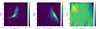 |
Fig. D.1. Unregularised KDE estimates for q in the left panel, n in the second panel, and q/n with logarithmic colour bar in the third panel. The KDE bandwidth of 0.2 stems from Barkus et al. (2022). |
Second, we changed the form of f(r). Theoretically, we might expect both the distance between the ‘true’ optical counterpart and the radio ridgeline ropt, ridge and the distance between the ‘true’ optical counterpart and the radio centroid ropt, centroid to be Rayleigh distributed24. However, as Fig. D.3 demonstrates, the lognormal distribution clearly provides the best empirical fit to the distances. The figure shows a histogram of the distance measures for RGs to their optical counterpart as manually identified through RGZ. Specifically, we plot the distances for the same 905 RGs, with an angular length ϕ > 1′, from 40 randomly selected pointings as above. Thus we update f(r) to be:
 (D.1)
(D.1)
where we empirically determined σ and μ using our sample of 905 RGs,
 (D.2)
(D.2)
and
 (D.3)
(D.3)
with n = 905 the size of our sample.
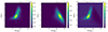 |
Fig. D.2. Regularised KDE estimates for q in the left panel, n in the second panel, and q/n with logarithmic colour bar in the third panel. The KDE bandwidth of 0.4 stems from 10-fold cross-validation. |
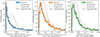 |
Fig. D.3. Each panel shows the histogram of a different distance measure between 905 radio galaxies with ϕ > 1′ and their optical host. The grey, dark grey, and black lines show empirical fits to these histograms for Rayleigh, normal, and lognormal distributions respectively. The tails of the histograms are long; for visualisation purposes we only plot the r-axis up to 0.05, 0.20, and 0.20. |
Appendix E: Sky coverages
As an extension of Sect. 4.9, this appendix details the sky coverages of our analyses. In particular, Table E.1 provides a decomposition – in terms of disjoint spherical quadrangles – of the sky coverage common between the ML pipeline, RGZ, and the combined manual search of Dabhade et al. (2020b) and Oei et al. (2023a). For simplicity, and as an acknowledgement of the wiggle room inherent to defining this joint sky coverage, we chose integer coordinates. Together, these spherical quadrangles cover Ω = 5327.9 deg2 = 1.62 sr (25.8%) of the Northern Sky. We refer to this coverage simply as the ‘LoTSS DR2 coverage’.
The RGZ–ML–Oei et al. (2023a) overlap region amounts to the LoTSS DR2 coverage with the LoTSS DR1 spherical quadrangle removed. The minimum and maximum right ascensions of this quadrangle are αmin = 160° and αmax = 230°, while its minimum and maximum declinations are δmin = 45° and δmax = 56°. This smaller overlap region covers 4838.9 deg2 (23.5%) of the Northern Sky. It is the sky coverage relevant to estimating the identification probability functions of Sect. 4.9.1 and Fig. 9: pobs, ID, 1(lp, z), pobs, ID, 2(lp, z), and pobs, ID(lp, z).
Sky coordinates and solid angles of disjoint spherical quadrangles whose union forms the LoTSS DR2 sky coverage – over which we have performed our inference. For each spherical quadrangle, we provide the minimum and maximum right ascension, αmin and αmax, the minimum and maximum declination, δmin and δmax, and its solid angle, Ω. We list the largest quadrangles first. The second and third quadrangle touch along the 360°–0° right ascension coordinate boundary, and could be viewed as a single whole.
All Tables
Sky coordinates and solid angles of disjoint spherical quadrangles whose union forms the LoTSS DR2 sky coverage – over which we have performed our inference. For each spherical quadrangle, we provide the minimum and maximum right ascension, αmin and αmax, the minimum and maximum declination, δmin and δmax, and its solid angle, Ω. We list the largest quadrangles first. The second and third quadrangle touch along the 360°–0° right ascension coordinate boundary, and could be viewed as a single whole.
All Figures
|
Fig. 1. Schematic of a three-method search for giants. Of all giants in the survey footprint up to z = zmax, only those for which the lobe surface brightness at the observing frequency νobs is above detection threshold bν, th are identifiable. 𝒢 denotes the actually identified set of giants. 𝒢1, 𝒢2, and 𝒢3 are the subsets identified by each method individually. As an example, we shade 𝒢2 ∪ 𝒢3, which has overlap with 𝒢1, and which can be used to measure pobs, ID, 1(lp, z). |
| In the text | |
|
Fig. 2. Overview of our approach, which consists of two stages. In the first stage we built a GRG sample, and in the second stage we inferred the properties of the intrinsic GRG population using a forward model. The brackets indicate the different parts of our approach and mention the sections containing the corresponding details. |
| In the text | |
|
Fig. 3. Summary of the angular length re-evaluation for radio source ILTJ130738.79+270355.1. Panels A–D show the initial cutout, the removal of neighbouring sources, the masking of emission outside a convex hull based on the old angular length, and the emission that is left after masking all emission below thrice the local noise σ. The red line segments delineate the convex hull of the left-over emission, and the red points indicate the furthest removed points in this convex hull. The great-circle distance between these points is the 3σ angular length. |
| In the text | |
|
Fig. 4. LoTSS DR2 cutouts at central observing frequency νobs = 144 MHz and resolution θFWHM = 6″, centred around the hosts of newly discovered giants. Each cutout covers a solid angle of 3′×3′. Contours signify 3, 5, and 10 sigma-clipped standard deviations above the sigma-clipped median. For scale, we show the stellar Milky Way disk (with a diameter of 50 kpc) generated using the Ringermacher & Mead (2009) formula, alongside a 3 times inflated version. Each DESI Legacy Imaging Surveys DR9 (g, r, z) inset shows the central 1′×1′ square region. As all giants obey ϕ ≥ 1.3′, they must – if not oriented along one of the square’s diagonals – necessarily protrude from this region. Rowwise from left to right, from top to bottom, these giants are ILTJ000212.45+222116.2, ILTJ001115.77+220316.6, ILTJ001350.25+324530.8, ILTJ001831.84+322247.7, ILTJ003025.90+334729.2, and ILTJ003534.45+221937.8. |
| In the text | |
|
Fig. 5. LoTSS DR2 cutouts at central observing frequency νobs = 144 MHz and resolution θFWHM = 6″, centred around the hosts of newly discovered giants. Each cutout covers a solid angle of 6′×6′. Contours signify 3, 5, and 10 sigma-clipped standard deviations above the sigma-clipped median. For scale, we show the stellar Milky Way disk (with a diameter of 50 kpc) generated using the Ringermacher & Mead (2009) formula, alongside a 3 times inflated version. Each DESI Legacy Imaging Surveys DR9 (g, r, z) inset shows the central 1′×1′ square region. As all giants obey ϕ ≥ 1.3′, they must – if not oriented along one of the square’s diagonals – necessarily protrude from this region. Rowwise from left to right, from top to bottom, these giants are ILTJ002943.72+295700.3, ILTJ003010.58+170948.6, ILTJ003521.87+233625.9, ILTJ003712.91+284436.8, ILTJ004002.30+252550.9, and ILTJ235802.49+331838.5. |
| In the text | |
|
Fig. 6. With 11 485 unique giants, we present the largest catalogue of large-scale galactic feedback to the Cosmic Web. The RGZ (orange) and ML pipeline (red) samples are strictly confined to the LoTSS DR2 area, while the sample by Oei et al. (2023a) extends to yet-to-be-released LoTSS pointings processed with the DR2 pipeline. |
| In the text | |
|
Fig. 7. Observed distributions of angular length ϕ, showing that our three LoTSS DR2 search methods target different ranges of ϕ. The largest angular lengths detected by Oei et al. (2023a), RGZ, and the ML pipeline are 132′, 43′, and 8′ respectively, but we limit the horizontal axis to 12′ for interpretability. The vertical line marks the minimum angular length that giants can attain: ϕGRG(lp, GRG = 0.7 Mpc) = 1.3′. |
| In the text | |
|
Fig. 8. Our sample of RGZ giants (orange squares) and ML pipeline giants (red squares) effectively complements the sample of giants with large angular lengths (blue dots) from the manual search of Oei et al. (2023a). The remaining giants (green pluses) are from earlier literature, as specified in Sect. 4.8. |
| In the text | |
|
Fig. 9. Overview of our determination of the probability to identify giants in the LoTSS DR2 with above-noise surface brightnesses, as a function of projected length and redshift – through Radio Galaxy Zoo: LOFAR and our machine learning pipeline (top row), through the search of Oei et al. (2023a, middle row), and through these methods in unison (bottom row). Each of the upper four panels shows a binary logistic regression following the theory of Sect. 2.4.2 and the practical considerations of Sect. 4.9.1. The left column shows results from all available data, whilst the right column shows results from rebalanced data. In our Bayesian inference, we used the latter results. |
| In the text | |
|
Fig. 10. Likelihood function over θ = [ξ(lp, GRG),Δξ, bν, ref, σref, ζ, nGRG], based on 2685 projected lengths and redshifts of giants up to zmax = 0.5. We show all two-parameter marginals of the likelihood function, with contours enclosing 50% and 90% of total probability. We mark the maximum likelihood estimate (MLE) values (grey dot) and the likelihood mean values (grey cross). The one-parameter marginals again show the MLE (dash-dotted line), a mean-centred interval of standard deviation–sized half-width (hashed region), and a median-centred 90% credible interval (shaded region). |
| In the text | |
|
Fig. 11. Empirical relation between projected proper length and two-lobe proper volume for RGs from Ineson et al. (2017), Oei et al. (2022, 2023b). The power law–like trend motivates Eq. (24). The green fit is based on giants only, whilst the grey fit is based on all RGs. VGRG is the mean two-lobe proper volume of the shortest possible giants (i.e. giants for which lp = lp, GRG), while γ is the exponent of the power law. For self-similar RG growth, γ = 3. |
| In the text | |
|
Fig. 12. Posterior distribution for the instantaneous, present-day GRG lobe volume-filling fraction in clusters and filaments of the Cosmic Web, 𝒱GRG − CW(z = 0). |
| In the text | |
|
Fig. D.1. Unregularised KDE estimates for q in the left panel, n in the second panel, and q/n with logarithmic colour bar in the third panel. The KDE bandwidth of 0.2 stems from Barkus et al. (2022). |
| In the text | |
|
Fig. D.2. Regularised KDE estimates for q in the left panel, n in the second panel, and q/n with logarithmic colour bar in the third panel. The KDE bandwidth of 0.4 stems from 10-fold cross-validation. |
| In the text | |
|
Fig. D.3. Each panel shows the histogram of a different distance measure between 905 radio galaxies with ϕ > 1′ and their optical host. The grey, dark grey, and black lines show empirical fits to these histograms for Rayleigh, normal, and lognormal distributions respectively. The tails of the histograms are long; for visualisation purposes we only plot the r-axis up to 0.05, 0.20, and 0.20. |
| In the text | |
Current usage metrics show cumulative count of Article Views (full-text article views including HTML views, PDF and ePub downloads, according to the available data) and Abstracts Views on Vision4Press platform.
Data correspond to usage on the plateform after 2015. The current usage metrics is available 48-96 hours after online publication and is updated daily on week days.
Initial download of the metrics may take a while.