| Issue |
A&A
Volume 672, April 2023
|
|
|---|---|---|
| Article Number | A163 | |
| Number of page(s) | 41 | |
| Section | Extragalactic astronomy | |
| DOI | https://doi.org/10.1051/0004-6361/202243572 | |
| Published online | 19 April 2023 | |
Measuring the giant radio galaxy length distribution with the LoTSS⋆
1
Leiden Observatory, Leiden University, Niels Bohrweg 2, 2300 RA Leiden, The Netherlands
e-mail: oei@strw.leidenuniv.nl
2
Somerville College, University of Oxford, Woodstock Road, Oxford OX2 6HD, UK
3
Centre for Astrophysics Research, University of Hertfordshire, College Lane, Hatfield AL10 9AB, UK
4
Observatoire de Paris, LERMA, Collège de France, CNRS, PSL University, Sorbonne University, 75014 Paris, France
5
Thüringer Landessternwarte, Sternwarte 5, 07778 Tautenburg, Germany
Received:
16
March
2022
Accepted:
24
October
2022
Context. Many massive galaxies launch jets from the accretion disk of their central black hole, but only ∼103 instances are known in which the associated outflows form giant radio galaxies (GRGs, or giants): luminous structures of megaparsec extent that consist of atomic nuclei, relativistic electrons, and magnetic fields. Large samples are imperative to understanding the enigmatic growth of giants, and recent systematic searches in homogeneous surveys constitute a promising development. For the first time, it is possible to perform meaningful precision statistics with GRG lengths, but a framework to do so is missing.
Aims. We measured the intrinsic GRG length distribution by combining a novel statistical framework with a LOFAR Two-metre Sky Survey (LoTSS) sample of freshly discovered giants. In turn, this allowed us to answer an array of questions on giants. For example, we can now assess how rare a 5 Mpc giant is compared with one of 1 Mpc, and how much larger – given a projected length – the corresponding intrinsic length is expected to be. Notably, we can now also infer the GRG number density in the Local Universe.
Methods. We assumed the intrinsic GRG length distribution to be Paretian (i.e. of power-law form) with tail index ξ, and predicted the observed distribution by modelling projection and selection effects. To infer ξ, we also systematically searched the LoTSS for hitherto unknown giants and compiled the largest catalogue of giants to date.
Results. We show that if intrinsic GRG lengths are Pareto distributed with index ξ, then projected GRG lengths are also Pareto distributed with index ξ. Selection effects induce curvature in the observed projected GRG length distribution: angular length selection flattens it towards the lower end, while surface brightness selection steepens it towards the higher end. We explicitly derived a GRG’s posterior over intrinsic lengths given its projected length, laying bare the ξ dependence. We also discovered 2060 giants within LoTSS DR2 pipeline products; our sample more than doubles the known population. Spectacular discoveries include the largest, second-largest, and fourth-largest GRG known (lp = 5.1 Mpc, lp = 5.0 Mpc, and lp = 4.8 Mpc), the largest GRG known hosted by a spiral galaxy (lp = 2.5 Mpc), and the largest secure GRG known beyond redshift 1 (lp = 3.9 Mpc). We increase the number of known giants whose angular length exceeds that of the Moon from 10 to 23; among the discoveries is the angularly largest known radio galaxy in the Northern Sky, which is also the angularly largest known GRG (ϕ = 2°). Combining theory and data, we determined that intrinsic GRG lengths are well described by a Pareto distribution, and measured the index ξ = −3.5 ± 0.5. This implies that, given its projected length, a GRG’s intrinsic length is expected to be just 15% larger. Finally, we determined the comoving number density of giants in the Local Universe to be nGRG = 5 ± 2(100 Mpc)−3.
Conclusions. We developed a practical mathematical framework that elucidates the statistics of giant radio galaxy lengths. Through a LoTSS search, we also discovered 2060 new giants. By combining both advances, we determined that intrinsic GRG lengths are well described by a Pareto distribution with index ξ = −3.5 ± 0.5, and that giants are truly rare in a cosmological sense: most clusters and filaments of the Cosmic Web are not currently home to a giant. Thus, our work yields new observational constraints for analytical models and simulations featuring radio galaxy growth.
Key words: galaxies: active / galaxies: jets / galaxies: kinematics and dynamics / radio continuum: galaxies / intergalactic medium
Table F.1 is only available at the CDS via anonymous ftp to cdsarc.cds.unistra.fr (130.79.128.5) or via https://cdsarc.cds.unistra.fr/viz-bin/cat/J/A+A/672/A163
© The Authors 2023
 Open Access article, published by EDP Sciences, under the terms of the Creative Commons Attribution License (https://creativecommons.org/licenses/by/4.0), which permits unrestricted use, distribution, and reproduction in any medium, provided the original work is properly cited.
This article is published in open access under the Subscribe to Open model. Subscribe to A&A to support open access publication.
1. Introduction
When gas, dust, and stars accrete onto a supermassive black hole (SMBH) in the centre of a galaxy, collimated jets arise along the Kerr rotation axis that blast some of the infalling material into the intergalactic medium (IGM) (e.g., Blandford & Rees 1974). In this process, the ejecta dissolve into a relativistic plasma that drags along a magnetic field and glows in synchrotron light. The resulting luminous structure is called a radio galaxy (RG); the central black hole that has generated it an active galactic nucleus (AGN).
It is increasingly clear that RGs and their AGN play an important role in galaxy evolution and cosmology. By heating the interstellar medium (ISM) or even expelling it from their host galaxies through galactic superwinds, AGN quench star formation (e.g., Di Matteo et al. 2005). Beckmann et al. (2017) have shown that AGN-induced star formation quenching is most pronounced in massive galaxies. There is also compelling evidence that the accompanying RGs provide the energy necessary to stop (e.g., McNamara & Nulsen 2012; Yang et al. 2019) bremsstrahlung-mediated cooling flows (Fabian et al. 1984) in clusters of galaxies. In the absence of cooling flows, the intra-cluster medium (ICM) remains dilute and hot, and galaxies in the centres of clusters are denied infalling gas that could otherwise reignite star formation. Cosmological simulations that include this RG feedback indeed resolve (e.g., Croton et al. 2006) the overprediction of baryonic masses and luminosities of central cluster galaxies that early simulations found. Finally, RGs may be responsible for magnetising the IGM that pervades the filaments of the Cosmic Web (e.g., Vazza et al. 2017).
Despite the emerging picture that RGs trace quenched star formation, inhibit cooling flows, and magnetise filaments, our knowledge of them is far from complete. Concerning geometry, a major unknown is the exact connection between the morphology of RGs and the pressure field of the ambient IGM, especially in filaments and cluster outskirts. Another question is whether small and large RGs come from the same initial population, or whether their growth is driven by distinct physical processes. Finally, we do not know how large can RGs become, and, more generally, how many RGs there are of each length.
To test RG growth models that answer these and other questions, it is imperative to study the subpopulation of most spatially extreme RGs: the giant radio galaxies (GRGs). The defining feature of giants is that their proper lengths – when projected onto the celestial sphere – exceed some threshold lp, GRG, which is canonically chosen as 0.7 Mpc or 1 Mpc. If lp, GRG = 0.7 Mpc, then the preceding literature describes a total of 1281 giants.
In recent years, several studies have successfully searched for giants in systematic, wide-area surveys such as the NRAO VLA Sky Survey (NVSS; Condon et al. 1998) and the LOFAR Two-metre Sky Survey (LoTSS; Shimwell et al. 2017). A combination of manual (i.e. visual) and automated searches (Solovyov & Verkhodanov 2011, 2014; Amirkhanyan 2016; Proctor 2016; Dabhade et al. 2017, 2020a) in the NVSS yielded 313 new giants (24% of the aforementioned literature population). Meanwhile, Dabhade et al. (2020b) discovered 225 new giants (17% of this same population) in the LoTSS DR1 (Shimwell et al. 2019), whose survey footprint is 80 times smaller than NVSS’s. Such searches have the advantage of introducing almost homogeneous selection effects throughout the survey footprint, which can potentially be modelled and thus corrected for during any subsequent statistical inference.
In this work this idea comes to fruition, by conducting a precision analysis of the intrinsic giant radio galaxy length distribution. To do so, we require two ingredients. First, in Sect. 2, we develop a statistical framework that allows one to answer probabilistic questions regarding both large samples of giants and individual specimina. Then, in Sect. 3, we describe our LoTSS DR2 (Shimwell et al. 2022) GRG search campaign and the trove of previously unknown giants it has yielded; moreover, we describe the assemblage of the most complete GRG catalogue to date. In Sect. 4, combining theory and data, we infer the tail index parameter that describes the intrinsic GRG length distribution, which constrains future models and simulations aimed at understanding RG growth. In Sect. 5, we discuss caveats of the current work and give recommendations for future extensions, before we present conclusions in Sect. 6.
We assume a concordance inflationary Λ cold dark matter cosmology with parameters 𝔐 from Planck Collaboration VI (2020); that is to say 𝔐 = (h = 0.6766, ΩBM, 0 = 0.0490, ΩM, 0 = 0.3111, ΩΛ, 0 = 0.6889), where H0 := h × 100 km s−1 Mpc−1. We define the spectral index α such that it relates to flux density Fν at frequency ν as Fν ∝ να, and define giants using threshold lp, GRG := 0.7 Mpc. Regarding the terminology, we use ‘angular length’ where others use ‘largest angular size’ (LAS), and ‘projected proper length’ where others use ‘largest linear size’ (LLS)1.
2. Theory
To measure the intrinsic GRG length distribution, we must first establish a suitable statistical framework. In this section, we provide a summary of the theory developed in Appendix A. Following Occam’s razor, we construct a model with minimal assumptions that provides new insight into the GRG phenomenon and the detection biases inherent to systematic search campaigns.
2.1. Intrinsic proper length
Firstly, we assume that giants and non-giant RGs share a common length distribution2. In particular, because power laws are abundant in Nature, we assume that the intrinsic proper length random variable (RV) L has a Pareto distribution with tail index ξ < −1 and support from lmin > 0 onwards. If an RV is Pareto distributed, then the relative occurrence of two possible outcomes equals their ratio raised to a power: the tail index ξ. In astrophysics, Pareto distributions describe the kinetic energies of freshly accelerated electrons in large-scale structure and supernova shocks (e.g., Kirk & Schneider 1987), the initial masses of main-sequence stars (e.g., Kroupa 2001), and the luminosities of gamma-ray bursts (e.g., Bloom et al. 2001), to name a few examples. Previous works (e.g., Andernach et al. 2021) have already hinted at the approximate validity of a Pareto distribution description for GRG lengths. By comparing our final model to observations, as discussed in Sect. 4 and visualised in Fig. 14, we demonstrate that this assumption is indeed a powerful approximation in the current case.
The probability density function (PDF) fL : ℝ → ℝ≥0 thus becomes
We refer the reader to Appendix A.1 for a derivation of this expression and a demonstration of its connection to the literature’s most common parametrisation.
2.2. Projected proper length
From the distribution of intrinsic lengths and the assumption of random radio galaxy orientations, we now derive the distribution of projected lengths. This distribution is more easily compared to observations, which usually lack inclination angle information.
2.2.1. Distribution for RGs
To model length and orientation, we consider a vector  (of length L := ||L||2) for each RG. In accordance with the IAU Solar System convention for positive poles, the unit vector
  marks the direction from which the central Kerr black hole is seen rotating in anticlockwise direction3. We define the inclination angle Θ as the angle between L and a vector parallel to the line of sight pointing towards the observer4. Observations that allow one to measure the orientation of the RG axis in 3D are time-intensive, and so usually only the RG length projected onto the plane of the sky is known.
Geometrically, we model RGs as line segments – as if they were ‘thin sticks’, with vanishing volumes – so that the projected proper length RV Lp relates to L and Θ through
We assume that  is drawn from a uniform distribution on 𝕊2, so that the PDF fΘ : [0, π]→ℝ≥0 becomes
  . Since L and Θ are independent, we find in Appendix A.2.1 that the PDF of Lp, fLp : ℝ → ℝ≥0, is
where
We note that for lp > lmin, the projected proper length has a Pareto distribution with the same tail index as the intrinsic proper length distribution. We compare fL and fLp in Fig. 1.
 |
Fig. 1. PDFs of radio galaxy intrinsic proper lengths L and projected proper lengths Lp. If the intrinsic lengths L are Pareto distributed above some cut-off lmin, then their projections on the sky Lp are also Pareto distributed above this cut-off. The tail indices are the same. We show the PDFs fL(left) and fLp(right) for lmin = 0.5 Mpc, lmax = ∞ (see Appendix A) and various tail indices ξ. The support of fL starts at lmin, which is marked by the vertical grey line in the right panel. |
2.2.2. Distribution for giants
For giants specifically (i.e. RGs such that Lp > lp, GRG, where lp, GRG is some constant threshold; in this work, lp, GRG := 0.7 Mpc), the projected proper length distribution becomes a Pareto distribution with tail index ξ again:
In other words, for giants, projection retains the Paretianity of lengths. A measurement of the tail index of the projected length distribution is immediately also a measurement of the tail index of the intrinsic length distribution.
The survival function, which gives the probability that a GRG has a projected proper length exceeding lp, takes on a particularly simple form:
The mean projected proper length of giants is the expectation value of Lp | Lp > lp, GRG:
which is only defined when ξ < −2. For example, when ξ = −4, ![$ \mathbb{E}[L_{\mathrm{p}}\ \vert\ L_{\mathrm{p}} > l_{\mathrm{p,GRG}}] = \frac{3}{2} l_{\mathrm{p,GRG}} $](/articles/aa/full_html/2023/04/aa43572-22/aa43572-22-eq12.gif) , which becomes 1.05 Mpc for lp, GRG := 0.7 Mpc and 1.5 Mpc for lp, GRG := 1 Mpc.
, which becomes 1.05 Mpc for lp, GRG := 0.7 Mpc and 1.5 Mpc for lp, GRG := 1 Mpc.
Appendix A.2.2 provides a derivation for all three expressions.
2.3. Deprojection factor
The deprojection factor,  , quantifies how much larger intrinsic lengths are compared with projected lengths. The PDF of D, fD : ℝ → ℝ≥0, is
The mean deprojection factor ![$ \mathbb{E}[D] = \frac{\pi}{2} $](/articles/aa/full_html/2023/04/aa43572-22/aa43572-22-eq15.gif) . Deprojection factors can become arbitrarily large under the current model, because projected lengths can become arbitrarily small. As discussed in Sect. 5.2, this is not a very realistic set-up. In reality, an RG’s projected length is bounded from below by its lobes, which have a non-vanishing volume and thus extend along all three spatial dimensions. Upon projection, the projected length therefore cannot shrink beyond some lower limit that depends on the lobe geometry. In Appendix A.3, we show that by enriching the conventional stick-like geometry with spherical lobes, deprojection factors indeed become bounded.
. Deprojection factors can become arbitrarily large under the current model, because projected lengths can become arbitrarily small. As discussed in Sect. 5.2, this is not a very realistic set-up. In reality, an RG’s projected length is bounded from below by its lobes, which have a non-vanishing volume and thus extend along all three spatial dimensions. Upon projection, the projected length therefore cannot shrink beyond some lower limit that depends on the lobe geometry. In Appendix A.3, we show that by enriching the conventional stick-like geometry with spherical lobes, deprojection factors indeed become bounded.
2.4. Intrinsic proper length posterior and its moments
Because an RG’s intrinsic length is more physically informative than its projected length, we ideally obtain the former. In this subsection, we quantify what a measurement Lp = lp already reveals about L.
We first note that the projected length bounds the intrinsic length from below. The intrinsic length can be much larger, however, but this is improbable for two reasons: large lengths are rarer than small lengths, although how drastic this effect is depends on ξ; in addition, viewing directions with large inclination angles are uncommon. The best we can do is to construct a posterior distribution for L given Lp = lp. This posterior has a concise analytic form. If lp > lmin, which is the relevant case for giants, the distribution of L | Lp = lp is
For l ≫ lp,  : the posterior PDF tends to a power law in l with index ξ − 2. In Fig. 2, we visualise the posterior PDF for several values of ξ.
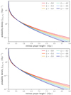 |
Fig. 2. Posterior PDFs of intrinsic lengths for a given projected length L | Lp = lp. If tail index ξ is known, then an RG’s lp fixes the probability distribution over its possible l. This distribution is strongly skewed, and the same for all lp – save for horizontal translation and vertical scaling. We illustrate this point by showing posterior PDFs for giants with two different lp. Top: lp = 1 Mpc. Bottom: lp = 5 Mpc. For ξ = −4, the posterior mean 𝔼[L | Lp = lp] = 1.13 lp and the posterior standard deviation |
Clearly, to evaluate Eq. (9), one must choose lp – however, the shape of the distribution is the same for all choices. We illustrate this by comparing the PDF for a comparatively small GRG (lp = 1.0 Mpc; top panel) to the PDF for Alcyoneus5 (lp = 5.0 Mpc; bottom panel).
The posterior mean is
the posterior variance is
Both mean and standard deviation scale linearly in lp: the projection effect is a multiplicative noise source. In Table 1, we provide explicit values for various ξ.
Intrinsic proper length posterior mean and standard deviation in multiples of projected proper length lp, given for various tail indices ξ.
Higher moments exist up to order ⌈ − ξ⌉; because the PDF fL | Lp = lp(l) is strongly skewed, such moments do further specify the distribution.
It is important to note that it is formally incorrect to statistically deproject RGs by drawing samples from deprojection factor D and multiplying them with some measurement Lp = lp, or even more crudely, by multiplying the latter with 𝔼[D]. The reason that renders such approaches invalid is that Lp = L sin Θ and D = sin−1Θ are not independent RVs. We refer to Appendix A.4 for an explicit proof of this fact, and for derivations of this subsection’s expressions.
2.5. GRG inclination angle
Radio galaxies with jets that make a small angle with the plane of the sky are more likely to have a projected length exceeding lp, GRG than those with jets that make a large angle with the plane of the sky. For this reason, the inclination angle distribution of giants is different from that of RGs: it is more peaked around θ = 90°. More precisely, the PDF fΘ | Lp > lp, GRG : [0, π]→ℝ≥0 of the GRG inclination angle Θ | Lp > lp, GRG has the general form
Under our Pareto distribution assumption for L, this concretises to
We note that fΘ | Lp > lp, GRG(θ)∝sin−ξθ; the factor in front serves only as a normalisation constant. The distribution is independent of the choice of lp, GRG and depends on a single parameter: ξ. We visualise fΘ | Lp > lp, GRG(θ) in Fig. 3.
 |
Fig. 3. PDFs of GRG inclination angles Θ | Lp > lp, GRG (colours) and RG inclination angles Θ (grey). Giants more often have orientations close to the sky plane. The strength of this tendency is governed by ξ, with larger ξ meaning more dispersion. |
Appendix A.5 contains a brief derivation.
2.6. GRG angular length
The model predicts the distribution of GRG angular lengths in the Local Universe up to comoving distance rmax. The GRG angular length RV Φ | Lp > lp, GRG relates to the GRG projected proper length RV Lp | Lp > lp, GRG and the comoving distance RV R as
(We note that this relation is valid only in a flat Friedmann–Lemaître–Robertson–Walker (FLRW) universe.) We also assume that the GRG number density is constant in the Local Universe. The PDF of Φ | Lp > lp, GRG has useful analytic forms under two different idealisations.
In a Euclidean universe, z(R) = 0, and the minimal GRG angular length  . Then
which is valid as long as ξ ≠ −4.
In an expanding universe at low redshifts, the Hubble–Lemaître law  holds; the Hubble distance
  . In this case,
Figure 4 shows GRG angular length PDFs under both idealisations.
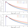 |
Fig. 4. PDFs of GRG angular lengths Φ | Lp > lp, GRG. We fix rmax = 1 Gpc (and lp, GRG = 0.7 Mpc), and vary ξ. Top: Euclidean universe. Bottom: expanding universe at low redshifts. |
The PDFs undergo a minor shift upon changing universe type but are otherwise similar. For most current-day applications, it will therefore be unnecessary to calculate an even more refined version of fΦ | Lp > lp, GRG(ϕ). Appendix A.6 contains derivations and details.
2.7. Maximum likelihood estimation of the tail index
The GRG projected proper length distribution features just one parameter of physical interest: the tail index ξ. If observational selection effects are negligible, one can directly use maximum likelihood estimation (MLE) on GRG data to infer ξ. In particular, we consider a set of projected lengths {Lp, 1, ..., Lp, N}∼Lp | Lp > lp, GRG from N giants. Appendix A.7 shows that the maximum likelihood estimate of ξ is the RV ξMLE, given by
2.8. Observed projected proper length
2.8.1. General considerations
In the preceding theory, we have ignored observational selection effects that favour some projected proper lengths over others. In practice, several such effects occur; the importance of each varies per survey and (G)RG search campaign within it. One of them is the bias against physically long RGs that the interferometer’s largest detectable angular scale can induce6. As a result, the projected proper length of an observed RG might not be adequately modelled through RV Lp. Instead, we must introduce a new RV Lp, obs.
We define the completeness C : ℝ> 0 × ℝ> 0 → [0,1] at (lp, zmax) to be the fraction of all RGs with projected proper length lp in the cosmological volume up to zmax that is detected in a particular RG search campaign. Then, assuming that the distribution of Lp does not evolve with redshift between z = zmax and z = 0 (i.e. ξ remains constant),
where pobs(lp, z) is the probability that an RG of projected proper length lp at cosmological redshift z is detected through the campaign, and r(z) is the comoving radial distance at cosmological redshift z. In a flat FLRW universe, the dimensionless Hubble parameter E is
The PDF of the observed projected proper length RV Lp, obs becomes
where we suppress the zmax-dependence for succinctness. We note that multiplying pobs(lp, z) with an lp- and z-independent factor affects the completeness C(lp, zmax), but cancels in Eq. (20); fLp, obs will be independent of it. Finally, the PDF of the GRG observed projected proper length RV Lp, obs | Lp, obs > lp, GRG is
We derive these expressions in Appendix A.8.1.
2.8.2. Fuzzy angular length threshold
We provide a concrete example of an important observational selection effect in visual searches for GRG candidates in survey images. To cope with the sheer number of detectable RGs in modern surveys like the LoTSS, a natural criterion is to only add sources to a candidate list if they appear – by eye – to have an angular length larger than some threshold. However, it is hard to precisely assess the angular length of a candidate before actually measuring it; sometimes, a candidate with a smaller angular length than the threshold will feature in the list, while some candidates with a larger angular length than the threshold will not. This leads to the notion of a ‘fuzzy angular length threshold’, where the probability that an RG with angular length ϕ is observed through the visual search increases (e.g., linearly) from 0 to 1 between ϕmin and ϕmax:
See the top row of Fig. 5 for several examples of associated completeness curves C(lp) and observed projected proper length PDFs. See Appendix A.8.2 for additional information.
 |
Fig. 5. Completeness functions (left column) and PDFs of observed projected proper lengths Lp, obs (right column). Selection effects leave imprints on the distribution of radio galaxies’ Lp, obs. In the top row, we show how imposing an angular length threshold in a GRG search campaign leads to incompleteness (left), which causes the PDF fLp, obs(right) to differ from fLp. We assume RGs with angular length ϕ < ϕmin have probability 0 to be included in a sample, whilst RGs with angular length ϕ > ϕmax have probability 1. The inclusion probability is assumed to increase linearly between ϕmin and ϕmax. In the left panel, we fix ϕmin = 3′ and vary ϕmax; in the right panel, we also fix ϕmax = 7′. In the bottom row, we show how a survey’s surface brightness limitations lead to incompleteness (left), which causes the PDF fLp, obs(right) to differ from fLp. We assume that lobe surface brightnesses are lognormally distributed; we parametrise the distribution for RGs of intrinsic length lref = 0.7 Mpc at z = 0 observed at νobs = 144 MHz with a median bν, ref and dispersion parameter σref. In the left panel, we fix σref = 1.5 and vary bν, ref; in the right panel, we also fix bν, ref = 1000 Jy deg−2. We assume a lobe spectral index α = −1, a surface brightness detection threshold bν, th = 25 Jy deg−2, and self-similar growth: ζ = −2. For both selection effects, we consider RGs up to cosmological redshift zmax = 0.5 only. |
2.8.3. Surface brightness limitations
Another important observational selection effect is due to a survey’s finite noise level. The noise determines the surface brightness threshold bν, th (typically comparable to the noise level itself) below which radio galaxy features remain visually undetected.
Fanaroff–Riley class II. We model the lobe surface brightness RV Bν at the central observing frequency νobs as
where bν, ref is the median surface brightness of RGs of intrinsic proper length lref at cosmological redshift z = 0 and frequency νobs, and S is a lognormally distributed RV with median 1 and dispersion parameter σref that captures the variability in surface brightness among this population of RGs. The denominator models the fact that surface brightness is not conserved with distance in an FLRW universe; Z is the cosmological redshift RV up to z = zmax and α is the typical lobe spectral index. The exponent ζ < 0 characterises the scaling between intrinsic proper length and surface brightness. (If RGs are self-similar, so that morphology does not predict length, one finds ζ = −2.) For this selection effect, the observing probability is
We note that pobs, SB does not depend on bν, th or bν, ref separately, but on their ratio only. See the bottom row of Fig. 5 for several examples of associated completeness curves C(lp) and observed projected proper length PDFs.
Fanaroff–Riley class I. For FRI RGs, the assumption of a constant surface brightness beyond the core is inaccurate. The simplest correction in which FRI RGs retain a well-defined notion of length assumes a linearly decreasing surface brightness profile, which peaks at the core and goes to zero at the RG’s two endpoints. (A power-law profile does not work: in such case, the surface brightness only goes asymptotically to zero – but never actually reaches it.) In this case, we define RV Bν to be the mean surface brightness along an RG’s jets, which can be regarded as a typical value for that RG. As Bν again obeys Eq. (24), we find that the formulaic structure of pobs, SB(lp, z) is identical for FRI and FRII giants, except that FRI giants require a change
which affects pobs, SB(lp, z) through smin. There is no change for lp = 2lp, GRG. Although the formulaic structure might be the same, the best-fit parameters can differ. For example, it is possible that σref, FRI ≠ σref, FRII or ζFRI ≠ ζFRII. See Appendix A.8.3 for derivations and numerical implementation considerations.
To include both aforementioned selection effects at the same time, a natural approximation is to assume that the observing probability simply factorises:
2.9. GRG number density
A central question in the field of radio galaxies is: how intrinsically rare are giants? By counting giants in a search campaign with well-understood selection effects, we can give an answer. More precisely, one can estimate the comoving number density of giants in the Local Universe, nGRG, through the number of observed giants up to cosmological redshift zmax in a uniformly searched region of sky of solid angle Ω, NGRG, obs(zmax,Ω). Then, under the standard assumption lp, GRG > lmin, Appendix A.9 shows that
Although the appropriate pobs(lp, z) varies per search campaign, it is always possible to bound pobs(lp, z) from above – for example by 1. In such case, Eq. (30) bounds nGRG from below.
2.10. GRG lobe volume-filling fraction
Because giants attain cosmological lengths, they might contribute to the energisation and magnetisation of Cosmic Web filaments in regions that smaller radio galaxies cannot reach. A key statistic that measures the enrichment of the Cosmic Web by giants is the volume-filling fraction (VFF) of their lobes. Assuming that lobes do not grow along with the expansion of the Universe, the proper VFF changes over cosmic time: VFFGRG(z) = VFFGRG(z = 0)⋅(1 + z)3, where
where V is the combined volume of the lobes and  is a dimensionless RV that captures the diversity in radio galaxy lobe shapes. We find under self-similar growth
𝔼[Υ] can be estimated from observations, but one must be wary of selection effects. Unfortunately, 𝔼[L3 | Lp > lp, GRG] does not exist for ξ ≥ −4, which is the regime supported by observations. A useful lower bound then is
where
This is the mean intrinsic proper length of giants, which is only defined when ξ < −2.7
An alternative is to deviate slightly from our Pareto ansatz and truncate the GRG projected proper length distribution at some lp, max; then
where  . See Appendix A.10 for a derivation and further details.
2.11. Unification model constraints from quasar and non-quasar giants
The unification model and its extensions (e.g., Hardcastle & Croston 2020) form an elegant family of hypotheses that aim to explain the observational diversity of active galaxies. It posits that active galaxies with quasars differ from those without quasars primarily because of differences in orientation of the dusty tori surrounding SMBHs. In particular, the central idea is that a quasar appears brighter to the observer than a non-quasar AGN because the axis of its dusty torus happens to be virtually parallel to the line of sight. As such, only quasars would offer an unobscured view of the luminous accretion disk surrounding the SMBH, whilst also beaming relativistic jet emission towards the observer. Using our statistical framework, we predict the general ramifications of the basic unification model on a GRG sample.
The basic unification model suggests to divide the radio galaxy population in two, distinguishing between RGs generated by AGN with quasar appearance (quasar RGs) and RGs generated by AGN without quasar appearance (non-quasar RGs). We assume that quasar RGs have inclination angles θ ≤ θmax or θ ≥ 180° −θmax whilst non-quasar RGs have θmax < θ < 180° −θmax8. If quasar RGs are more closely aligned with the line of sight than non-quasar RGs but are otherwise similar, fewer of them will satisfy lp ≥ lp, GRG and thus be classified as giants. Therefore, the quasar GRG fraction fQ – the fraction of quasar giants in an actual GRG sample – constrains θmax. We model fQ as an RV:
where the RV NQ is the number of quasar giants in the sample, the constant N is the total number of giants in the sample and the parameter pQ is the quasar GRG probability. Our framework predicts
See Appendix A.11 for a derivation. Interestingly, as long as quasar giants and non-quasar giants are subject to the same selection effects, these selection effects do not affect pQ.
Figure 6 shows that, for all relevant ξ, pQ is a steeply and monotonically increasing function of θmax. Thus, knowing ξ, one can use an empirical fQ to determine pQ and in turn θmax.
 |
Fig. 6. Probability pQ that an observed giant is a quasar giant under the unification model. Under this model, giants generated by AGN with quasar appearance (quasar giants) have inclination angles θ ≤ θmax or θ ≥ 180° −θmax and giants generated by AGN without quasar appearance (non-quasar giants) have intermediate θ. As long as quasar giants and non-quasar giants are subject to the same selection effects, these selection effects do not affect pQ. Instead, in such case, pQ only depends on the maximum quasar inclination angle θmax and the tail index ξ. |
Does one expect quasar giants to have a different distribution for Lp, obs | Lp, obs ≥ lp, GRG than non-quasar giants? Interestingly, our framework allows us to prove that the inclination angle differences between the two classes affect their relative rarity, but not their observed projected proper length distribution. Under the basic unification model, quasar giants and non-quasar giants obey the same Lp, obs | Lp, obs ≥ lp, GRG if they are subject to the same selection effects.
2.12. Extreme giants in a sample
The model can predict the occurrence of giants with extreme projected proper lengths in a sample of cardinality N. The probability that an observed GRG has a projected proper length exceeding lp is
so that the number of observed giants with a projected proper length exceeding lp is N> lp ∼ Binom(N, p> lp). Its expectation is 𝔼[N> lp]=N ⋅ p> lp. Furthermore, the probability that the sample contains at least one giant with projected proper length lp or higher is
See Appendix A.12 for details. Figure 7 shows 𝔼[N> lp] and ℙ(N> lp ≥ 1) for various ξ. As an example, the case ξ = −3.0 predicts that a sample of N = 1000 giants with redshifts below zmax = 0.5 should contain almost ten giants of lp > 5 Mpc, and still several of lp > 6 Mpc. Such predictions are useful as they can be directly compared to elementary sample statistics.
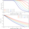 |
Fig. 7. Predictions of the existence and expected number of giants that exceed projected length lp in a sample of cardinality N, as functions of lp. Both tail index ξ and selection effect parameters affect these predictions. We consider a sample of N = 1000 giants with redshifts below zmax = 0.5, use ϕmin = 3′, ϕmax = 7′, bν, ref = 1000 Jy deg−2, and σref = 1.5, and keep other parameters as in Fig. 5. Top: the probability that at least one observed giant has a projected length of at least lp. Bottom: the expected number of observed giants with a projected length of at least lp. |
3. Sample compilation and properties
To measure the intrinsic GRG length distribution, we also require a large sample of giants collected from a single survey through a systematic approach. This ensures approximately homogeneous selection effects, which we can correct for in subsequent analysis using the statistical framework of Sect. 2.
3.1. LoTSS DR2
The Low-Frequency Array (LOFAR; van Haarlem et al. 2013) is a powerful, Pan-European radio interferometer that features both (sub)arcsecond-scale resolution and sensitivity to degree-scale structures. Dabhade et al. (2020b) have already demonstrated that this combination is ideal for detecting giants: these authors found a record 225 new specimina in the LoTSS DR1, the first data release of the LOFAR’s Northern Sky survey at central frequency νobs = 144 MHz.9 Excitingly, the recent LoTSS DR2 (Shimwell et al. 2022) improves the data calibration and increases the survey footprint from 424 deg2 to 5635 deg2 – that is by more than a factor 13. By default, the LoTSS features imagery at 6″ and 20″ resolutions. To further facilitate the discovery of giants (among other goals), we reprocessed the LoTSS by subtracting compact sources and imaging at 60″ and 90″ resolution; more details are given in Oei et al. (2022a, and in prep.). This 60″ and 90″ imagery has turned out to be effective in highlighting jets and lobes of RGs of large angular and physical extent, whose surface brightnesses are low and which therefore have remained undetected in shallower surveys, and even in the LoTSS DR2 at higher resolutions. We demonstrate this fact in Fig. 8 by comparing the LoTSS DR2 at 6″ and 60″ for three giants whose discovery has relied on the lower-resolution images. After the serendipitous discovery of several such hitherto unknown giants in the 60″ and 90″ images, we decided to initiate a systematic, multi-resolution, visual GRG search through the area covered by LoTSS DR2 pipeline products as of September 202210. This search comprised of a hundreds-of-hours-long inspection of the LoTSS maps at 6″ and 60″, alongside Pan-STARRS DR1 (Chambers et al. 2016) and SDSS DR9 (Ahn et al. 2012) maps, in Aladin Desktop 11.0 (Bonnarel et al. 2000).
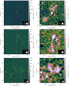 |
Fig. 8. LoTSS DR2 cutouts of three newly discovered giants at 6″ (left column) and 60″ (right column). By subtracting compact sources from calibrated 144 MHz visibility data and imaging at low resolution (60″ and 90″), we reveal otherwise speculative giant radio galaxies at the unexplored ∼1 Jy deg−2 surface brightness level. The claimed host galaxy is in the image centre. Top: a GRG of projected proper length lp = 1.4 ± 0.3 Mpc, whose angular length ϕ = 32.3 ± 0.2′ is larger than that of the full Moon. Middle: a GRG of lp = 1.6 ± 0.6 Mpc and ϕ = 16.4 ± 0.2′. Bottom: a GRG of lp = 3.6 ± 0.1 Mpc and ϕ = 8.5 ± 0.2′. For scale, we show the stellar Milky Way disk (with a diameter of 50 kpc) generated using the Ringermacher & Mead (2009) formula, alongside a 3, 5, or 10 times inflated version. |
Reliable automated search strategies do not yet exist for several reasons. Giants showcase a rich morphological variety (see Sect. 3.6) and are easily confused with other types of astrophysical sources (see Sects. 3.3 and 3.4). Moreover, the known population is too small to effectively apply supervised learning techniques. However, it appears possible to find giants in morphological outlier lists of unsupervised learning techniques such as self-organising maps (SOMs; Mostert et al. 2021). The efficacy of such techniques in GRG searches has not yet been quantified.
3.2. Angular length threshold
To limit the amount of manual work, we decided to search only for GRG candidates whose angular length exceeds some threshold. In Fig. 9, we show how the angular length ϕ of giants with six different projected proper lengths lp varies as a function of cosmological redshift z. Because of the expansion of the Universe, giants have an arcminute-scale minimum angular length: if lp, GRG = 0.7 Mpc, all giants obey ϕ > 1.3′11. For the purpose of finding a GRG, it is therefore never useful to inspect a source with an angular length less than 1.3′. Our highest priority has been to find giants with z < 0.2, which lie in a volume for which the total matter density field is known or will be known in the coming years through the combined power of deep spectroscopic surveys and Bayesian inference frameworks, such as the Bayesian Origin Reconstruction from Galaxies (BORG; Jasche & Wandelt 2013; Jasche et al. 2015; Jasche & Lavaux 2019). In an upcoming publication, we combine a sample of low-redshift giants with the BORG to analyse the large-scale environments of giants (Oei et al., in prep.). Figure 9 shows that all giants with lp > 1 Mpc at z < 0.2 have an angular length ϕ > 5′. For this reason, we have chosen 5′ as the angular length threshold of our search campaign. This choice has kept the visual inspection duration to order ∼102 h, while still enabling us to target all Mpc-exceeding giants in the Local Universe (z < 0.2). In practice, this threshold is ‘fuzzy’: it is hard to accurately estimate angular lengths by eye before performing an actual measurement, so that our list of GRG candidates does contain some with a smaller angular length than the specified threshold. Inversely, it will presumably lack some GRG candidates with an angular length exceeding the threshold.
 |
Fig. 9. Relations between cosmological redshift z and angular length ϕ for six giants of different projected lengths lp. Due to the expansion of the Universe, there is a minimum angular length for each lp. If one defines giants as RGs with lp ≥ lp, GRG = 0.7 Mpc, all giants have an angular length of 1.3′ or above. If one instead defines giants as RGs with lp ≥ lp, GRG = 1 Mpc, all giants have an angular length of 1.9′ or above. |
3.3. GRG candidates in the radio
We first identified GRG candidates in the LoTSS at 6″ and 60″. These maps serve complementary roles. The 6″ images reveal the precise morphology of radio galaxy cores and jets, which are necessary to pinpoint the host galaxy. Figure 10 provides a representative sense of the host galaxy identification accuracy these data allow for when combined with modern optical surveys such as the DESI Legacy Imaging Surveys (Dey et al. 2019) DR9. In contrast, the 60″ images have such compact sources removed or highly suppressed, but better highlight diffuse structures, such as RG lobes. Being similar in morphology, we made sure not to interpret diffuse emission from low-redshift spiral galaxies and their circumgalactic media, or radio halos and relics in galaxy clusters, as RG lobe emission. We required that all new RGs feature a detection of at least two12 lobes, or of at least one lobe and one jet oriented towards the lobe(s), at least one of the resolutions used in this work (6″, 20″, 60″, and 90″).
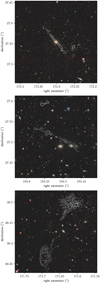 |
Fig. 10. 12′×12′ DESI Legacy Imaging Surveys DR9 (g, r, z)-details with LoTSS DR2 6″ contours (3σ, 5σ, 10σ) overlaid. At 6″ resolution, LoTSS images allow for more accurate host galaxy identification in SDSS, Pan-STARRS, and Legacy Survey images than was possible before. Top: the jet of the giant at rank 33 of Table 2 and shown in the middle-left panel of Fig. B.1. Middle: the giant at rank 37 of Table 2. Bottom: the giant at rank 43 of Table 2. |
3.4. GRG candidates in the optical
To confirm that a radio structure really is a radio galaxy, we compared the radio images with optical images of the same sky region. If a patch of radio emission is indeed due to RG jets or lobes, the patch itself must have no codirectional galactic counterpart in the optical. If the radio emission is due to a low-redshift spiral galaxy or a galaxy cluster instead, a corresponding easily recognisable counterpart will exist. We also took care not to erroneously associate the lobes of two distinct RGs. For this reason, we were more cautious to associate a pair of lobes to a suspected host galaxy when, in the optical, one could discern other galaxies in the angular vicinity of the lobes that could have generated them instead.
The Pan-STARRS and SDSS images used for these purposes complement each other, as they differ in quality throughout the sky – and in particular around sources of high optical flux density. Neither consistently outperforms the other. Only Pan-STARRS covers the full Northern Sky and could thus always be relied upon.
3.5. Host galaxy identification
We also used the Pan-STARRS and SDSS maps for the identification of host galaxies. We collected host redshifts from the SDSS DR12 (Alam et al. 2015) and Gaia (Gaia Collaboration 2016) DR3 (Gaia Collaboration 2021) through automated VizieR queries, from the Galaxy List for the Advanced Detector Era (GLADE) 2.4 (Dálya et al. 2018), and from the DESI DR9 photometric redshift catalogue (Zou et al. 2022). If redshifts from multiple sources were available, we favoured SDSS over GLADE data, GLADE over Gaia data, and Gaia over DESI data. Similarly, we only adopted photometric redshifts if spectroscopic ones were not available.
For a small subset of RGs, a definite host galaxy could not be established beyond reasonable doubt, but a set of candidates containing the host galaxy could. In these cases, the lowest-redshift candidate provides a lower bound to the RG’s projected proper length13. If this lower bound exceeds lp, GRG = 0.7 Mpc, then the actual projected proper length certainly does so too, and the RG can be classified as a GRG – despite persisting uncertainty concerning the identity of the host galaxy.
3.6. LoTSS DR2 GRG sample
Our search campaign has led to the identification of 2060 hitherto unknown giants. To establish novelty, we assembled a literature catalogue with all known giants as of September 2022, combining the catalogue of Dabhade et al. (2020a)14 with the giants discovered in Galvin et al. (2020), Ishwara-Chandra et al. (2020), Tang et al. (2020), Bassani et al. (2021), Brüggen et al. (2021), Delhaize et al. (2021), Masini et al. (2021), Kuźmicz & Jamrozy (2021), Andernach et al. (2021), Mahato et al. (2022), Gürkan et al. (2022), and Simonte et al. (2022). Fusing our sample with this literature catalogue, we obtain a final catalogue with N = 3341 giants.
Figure 11 shows the locations of all known giants in the sky. We list basic properties of the 50 projectively largest new discoveries in Table 2, and refer to Appendix F for access to these data for our entire sample. In Fig. 12 and Figs. B.1–B.3, we present images for discoveries with projected proper lengths lp in the ranges 5.1–4 Mpc, 4–3 Mpc, 3–2 Mpc, and 2–0.7 Mpc, respectively. For each giant, we use the LoTSS resolution θFWHM ∈ {6″, 20″, 60″, 90″} that most clearly conveys the morphology through a single image. The selection reflects our sample’s diversity in shapes and sizes and provides a sense of the data quality.
 |
Fig. 11. Mollweide view of the sky showing locations of all known giants, of which 62% are discoveries presented in this work. In the background, we show the specific intensity function of the Milky Way at νobs = 150 MHz (Zheng et al. 2017). The LoTSS DR2 has avoided the Galactic Plane, where extended emission complicates calibration and deconvolution. Our search footprint encloses a grey spherical rectangle, which represents the LoTSS DR1 search by Dabhade et al. (2020b), and a grey spherical cap, which represents the Boötes LOFAR Deep Field search by Simonte et al. (2022). |
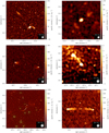 |
Fig. 12. Details of the LoTSS DR2–estimated specific intensity function |
Properties of the 50 projectively longest giants out of a total of 2060 discovered during our LoTSS DR2 search campaign.
3.6.1. Angular lengths
The angular length distribution of the newly found giants is as follows: the smallest ϕ = 1.5′, the median ϕ = 5.2′, the largest ϕ = 2.2°, and 80% of angular lengths fall within [3.4′,9.8′]. Thirteen of our discoveries – listed in Table 3 – are larger than the Moon in the sky (whose angular diameter varies over time, but here taken to be ϕ = 30′). Our search more than doubles the known number of such spectacular giants – from 10 to 23.
The GRG associated with NGC 2300 (see the middle-left panel of Fig. 13) is the giant with the largest angular length ever found, and the radio galaxy with the largest angular length in the Northern Sky15. It remains possible that the GRG has been generated by spiral galaxy NGC 2276 instead, with which elliptical galaxy NGC 2300 is interacting. However, this scenario seems unlikely, as only a fraction ∼10−3 of known giants are hosted by spirals. Its discovery emphasises that low-frequency interferometers like the LOFAR and the MWA, which are sensitive to degree-scale angular scales, are important to complete a low-redshift census of giant radio galaxies. Sky-wide, a simple extrapolation of our findings suggests that several (∼101) degree-scale angular length giants similar to the GRG of NGC 2300 still await discovery at the LoTSS DR2 depth.
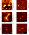 |
Fig. 13. Details of the LoTSS DR2–estimated specific intensity function |
3.6.2. Redshifts
The redshift distribution of the newly found giants is as follows: the lowest z = 0.00635 ± 6 × 10⁻⁵, the median z = 0.29, the highest z = 2.6394 ± 6 × 10⁻⁴, and 80% of redshifts fall within [0.12, 0.68]. Because of our focus on giants of large angular length (see Sect. 3.2), we have found only 36 giants beyond z > 1. One of these, the GRG at rank 13 of Table 2, is the largest secure giant found beyond redshift 1. It lies at z = 1.1 ± 0.1 and spans lp = 3.9 ± 0.1 Mpc. Its host galaxy does not appear to contain a quasar.
3.6.3. Projected proper lengths
With lp = 5.1 ± 0.2 Mpc and lp = 4.99 ± 0.04 Mpc, our LoTSS DR2 sample contains the first two 5 Mpc–scale giants. We have presented a dedicated analysis of the latter GRG in Oei et al. (2022a). 11 discoveries have lp ≥ 4 Mpc, 53 have 3 ≤ lp < 4 Mpc, 291 have 2 ≤ lp < 3 Mpc, 1215 have 1 ≤ lp < 2 Mpc, and 490 have 0.7 ≤ lp < 1 Mpc. The median lp = 1.35 Mpc, and 80% of projected proper lengths fall within [0.82 Mpc, 2.29 Mpc].
3.6.4. Stellar and supermassive black hole masses
Following Oei et al. (2022a), we collected host stellar masses M⋆ from Chang et al. (2015) and Salim et al. (2018), and estimated host SMBH masses M• via SDSS DR12 stellar velocity dispersions (Alam et al. 2015) and the M-sigma relation of Kormendy & Ho (2013)’s Eq. (7). From all 3341 giants in our final catalogue, only 732 (22%) could be assigned a stellar mass in this way, and only 1115 (33%) an SMBH mass; for both quantities, our LoTSS DR2 sample accounts for four-fifths of the resulting subpopulation. Figure C.1 shows both M⋆ and M• in relation to projected proper length lp.
The median M⋆ = 3.4 × 10¹¹ M⊙, and 80% of stellar masses fall within [1.8 × 10¹¹ M⊙, 5.3 × 10¹¹ M⊙]. We discover two giants whose hosts, J150329.07+374850.3 and J073505.24+415827.5, are the least massive known: both have a stellar mass M⋆ = 4.8 × 10¹⁰ M⊙. These are small giants, with lp = 0.8 Mpc and lp = 0.7 Mpc, respectively. The top panel of Fig. C.1 hints at a weak positive correlation between M⋆ and lp, which future work should confirm or reject.
The median M• = 1.0 × 10⁹ M⊙, and 80% of SMBH masses fall within [0.4 × 10⁹ M⊙, 2.2 × 10⁹ M⊙]. The SMBH masses of J123703.24+275819.5, J163659.07+541725.4, and J103129.54+502959.1 are the highest estimated yet, with M• = 2 × 10¹¹ M⊙, M• = 5 × 10¹⁰ M⊙, and M• = 5 × 10¹⁰ M⊙, respectively. The latter masses equal the theoretical maximum mass of accreting black holes of typical spin (King 2016). Curiously, although J103129.54+502959.1’s M• is among the highest estimated SMBH mass of any GRG host, the GRG itself is relatively small: lp = 0.81 ± 0.06 Mpc. Conversely, the bottom panel of Fig. C.1 shows that multi-Mpc giants can have hosts with SMBH masses that are two orders of magnitude lower than J103129.54+502959.1’s.
3.6.5. Spiral or lenticular host galaxies
Remarkably, although NGC 6185 is a spiral galaxy of Hubble–de Vaucouleurs class SAa (Jansen et al. 2000), it appears to have generated the giant shown in the top-left panel of Fig. 13. Such systems are exceedingly rare: not only are few RGs giants, but also virtually all giants have an elliptical galaxy as their host. With lp = 2.54 ± 0.01 Mpc, this is the largest known spiral galaxy–hosted radio galaxy. Hitherto, the largest spiral galaxy–hosted giant in the literature has been J2345-0449 (Bagchi et al. 2014), with lp = 1.6 Mpc. Given the favourably low redshift of z = 0.03430 ± 7 × 10⁻⁵, NGC 6185 and its enigmatic giant solicit a dedicated analysis (Oei et al. 2023). Besides NGC 6185, spiral or lenticular galaxies J080403.40+404809.3 and J091459.66+294348.8 (known alternatively as NGC 2789; see the bottom-right panel of Fig. 13) have also generated giants; these have projected proper lengths lp = 1.1 Mpc and lp = 0.9 Mpc, respectively. Morphological host classification through SDSS, Pan-STARRS, and DESI imagery is reliable only up to z ∼ 0.1–0.2, depending on viewing angle and various other factors. Our LoTSS DR2 sample contains 342 giants with definite hosts at z = 0.15 or below, among which are all 3 giants with spiral or lenticular hosts discussed here. It thus appears that the fraction of GRG hosts that is of such non-elliptical nature is ∼1%. A more detailed morphological characterisation of the sample appears possible, for example using data from Hart et al. (2016), but this is beyond the scope of the current work.
4. Results
After first building a statistical framework and then collecting a large sample of giants from a single survey through a systematic approach, we were ready to infer the intrinsic GRG length distribution. In particular, we aimed to establish whether the RG intrinsic proper length RV L is well described by a Pareto distribution, and if so, what its tail index ξ is. Subsequently, we inferred derived quantities, such as the comoving GRG number density in the Local Universe.
4.1. Giant radio galaxy length distribution
4.1.1. Empirical survival function
From our LoTSS DR2 GRG sample, we computed the empirical cumulative distribution function (ECDF) of the GRG observed projected proper length RV Lp, obs | Lp, obs > lp, GRG (see Eq. (21)). We only included giants for which lp itself – rather than a lower bound – is known, and set either zmax = 0.5 or zmax = 0.25; this retained 1473 or 811 giants for analysis, respectively16. The empirical survival function (ESF), which equals one minus the ECDF, is shown in dark grey in both panels of Fig. 14. Just as the ECDF approximates the CDF, the ESF approximates the survival function (SF). In this case, for any lp, the ESF provides the probability that a randomly drawn LoTSS DR2 GRG will have a projected proper length exceeding lp. If Lp, obs | Lp, obs > lp, GRG were Paretian, its ESF (hereafter: ‘the’ ESF) would resemble a straight line in Fig. 14’s right panel – both axes have logarithmic scaling. However, the ESF clearly displays curvature.
 |
Fig. 14. Empirical survival function of the observed giant radio galaxy projected proper length RV (ESF; dark grey) and the corresponding survival function 1 − FLp, obs | Lp, obs > lp, GRG (SF; green curve) using the maximum a posteriori probability parameters (MAP; see Table 4). Observed GRG projected lengths are well described by a Pareto distribution modified to include selection effects. Keeping the selection effect parameters fixed, we show how models vary with tail index ξ (green range). We also show the selection effect–free SF 1 − FLp | Lp > lp, GRG using the MAP ξ (green dots). We included all LoTSS DR2 search campaign giants up to zmax = 0.5. Left: logarithmic horizontal axis and linear vertical axis. Right: logarithmic horizontal axis and logarithmic vertical axis. |
4.1.2. Selection effects
Under the ansatz that L is Paretian, as proposed in Sect. 2.1, the aforementioned ESF’s curvature implies a significant role for observational selection effects. The reason is the following. The ansatz implies that the GRG projected proper length RV Lp | Lp > lp, GRG is also Paretian (see Eq. (5)), as is Lp, obs | Lp, obs > lp, GRG when selection effects are negligible (see Sect. 2.8.1 and set C(lp) = 1). But in our case Lp, obs | Lp, obs > lp, GRG is not Paretian: its ESF is curved. To avoid contradiction, we must relax at least one assumption. If the Pareto ansatz is held, then selection effects must be at play.
When selection effects are non-negligible, we must devise a procedure to disentangle them from the data if our ξ estimate is to be uncontaminated. To this end, we performed joint Bayesian inference with a model that includes both ξ and parameters that describe the selection effects.
In particular, we considered the roles of the fuzzy angular length threshold and surface brightness selection effects, introduced in Sects. 2.8.2 and 2.8.3, respectively. In Sect. 3.2, we explain that we have attempted to maintain a 5′ angular length threshold during our LoTSS DR2 GRG search. If we want to use Sect. 2.8.2 to correct for the bias against faraway and physically small giants that this threshold has imprinted onto our sample, we must estimate parameters ϕmin and ϕmax. A natural choice is to assume that they lie symmetrically around the intended angular length threshold of 5′ – but at what distance from it? We propose to consider this distance,  , as a yet unknown model parameter that we fitted to the data. Similarly, if we want to use Sect. 2.8.3 to correct for the bias against physically large giants that the limited depth of the LoTSS DR2 imprints onto our sample, we must estimate parameters bν, ref and σref. Our approach was to, again, fit these parameters – possibly making use of any available prior knowledge.
The meaning of bν, ref depends on the choice of lref and νobs; we defined lref := 0.7 Mpc and used νobs = 144 MHz. We furthermore assumed bν, th = 1 × σIν, with σIν = 25 Jy deg−2 being the typical LoTSS DR2 6″ RMS noise (Shimwell et al. 2022).
4.1.3. Prior
We exploited two sources of prior knowledge. Firstly, we attempted to directly estimate bν, ref and σref by selecting from all LoTSS DR2 giants with lp ≤ 1 Mpc a random subset of size 50 (10%). For these giants, we estimated the mean surface brightnesses of both lobes from the LoTSS DR2 6″ imagery, differentiating between the brighter and the fainter lobe. Because our goal was to estimate bν, ref, we attempted to undo cosmological and growth-induced surface brightness dimming assuming a universal lobe spectral index α = −1 and self-similar growth: ζ = −2. The resulting surface brightnesses correspond to z = 0, and to the epoch in each giant’s life when l = lref. The median of the corrected bright lobe mean surface brightnesses is bν, ref = 1.3 × 10³ Jy deg−2, whilst the median of the corrected faint lobe mean surface brightnesses is bν, ref = 0.7 × 10³ Jy deg−2. All lobes taken together, the median becomes bν, ref = 1.0 × 10³ Jy deg−2. We performed maximum likelihood estimation assuming the surface brightness distribution is lognormal and found σref = 1.3, again using all lobes. Note, however, that we have only used observed giants here, whilst bν, ref and σref should correspond to the entire population of giants. As fainter giants will have preferentially fallen out, we might have overestimated bν, ref and underestimated σref.
To probe whether we had overestimated bν, ref and underestimated σref, we used data from Dabhade et al. (2020b) and a Monte Carlo approach. First, for their sample of 239 LoTSS DR1 giants, we computed total luminosity densities Lν at rest-frame frequency ν = 144 MHz. (Given that LoTSS DR1 and DR2 noise levels are similar, this population is also representative of the LoTSS DR2.) In the top panel of Fig. 15, we show Lν versus lp for all 139 for which z < 0.6. To increase the range of lengths covered, we additionally show data on Alcyoneus (Oei et al. 2022a). Next, under the same assumptions of a constant spectral index and self-similar growth, we derived a simple luminosity density–surface brightness relationship that allows for back-and-forth conversion between the two – at least, given projected lengths and redshifts. The mean lobe surface brightness ⟨bν⟩ is proportional to the total luminosity density Lν, and assuming a pair of spherical lobes
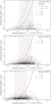 |
Fig. 15. Comparison between luminosity density–projected proper length relations for observed and simulated giants. Each dash-dotted curve denotes a family of giants at a given redshift, assuming fLν = 0.3 and fl = 0.3, whose mean lobe surface brightnesses equal the LoTSS DR2 noise level and who are thus borderline-detectable. The grey band denotes the median-centred luminosity density range that contains 68% of giants. Top: 139 LoTSS DR1 giants (Dabhade et al. 2020b), alongside Alcyoneus, with redshift zAlc. = 0.25 (Oei et al. 2022a). The solid green curve is similar to the dash-dotted green curve, but represents maximum instead of mean lobe surface brightness. Middle: 1000 simulated giants, assuming bν, ref = 1750 Jy deg−2 and σref = 1.3. Bottom: 1000 simulated giants, assuming bν, ref = 250 Jy deg−2 and σref = 1.3. |
Here fLν is the fraction of the total luminosity density that belongs to the lobes, fl is the fraction of the RG’s axis length that lies inside the lobes, and 𝔼[D](η(fl)) is the mean deprojection factor as given by Eq. (A.29). The peak surface brightness bν, max relates to ⟨bν⟩ as  . Appendix D contains derivations for both these results. For Alcyoneus, at zAlc. = 0.25, fLν = 0.3 and fl = 0.3 (Oei et al. 2022a). Assuming these parameter values, again in the top panel of Fig. 15, we show luminosity density–projected length pairs of RGs at z = zAlc. whose peak (solid green curve) or mean (dash-dotted green curve) surface brightness equals the LoTSS DR2 noise level. Thus, each curve represents a family of borderline-detectable giants at Alcyoneus’s redshift. The other dash-dotted curves indicate similar barely detectable families, but for other redshifts. Without optimising any free parameters, the curves correctly predict that Alcyoneus’s lobes have surface brightnesses comparable to the 6″ LoTSS DR2 noise level and explain the absence of observations in the top-left corner of the figure. We conclude that Eq. (40) appears reasonable, but note that RGs may significantly differ in their values of fLν and fl.17
Bolstered, we made use of Eq. (40) to Monte Carlo simulate – for particular values of bν, ref and σref – luminosity density–projected length relationships as they appear to observers. The simulated giants have projected lengths adopted from the observed giants, randomly sampled redshifts up to z = 0.6 assuming a spatially constant GRG number density, and randomly sampled reference surface brightnesses (i.e. those for RGs at z = 0 that have intrinsic length l = lref) whose distribution is determined by bν, ref and σref. We then used Eq. (24) to compute surface brightnesses as they would be observed, and retained only those giants whose surface brightness exceeds the LoTSS DR2 noise level. For these simulated detectable giants, we finally generated luminosity densities using Eq. (40), assuming wide uniform distributions fLν ∼ fl ∼ Uniform(0.1, 0.9). The middle and bottom panels of Fig. 15 show results for bν, ref = 1750 Jy deg−2 and bν, ref = 250 Jy deg−2, respectively; we adopted σref = 1.3 from our LoTSS DR2 GRG surface brightness measurements. The median luminosity density of the z < 0.6 LoTSS DR1 giants is Lν = 1.1 × 1026 W Hz−1, that of the bν, ref = 1750 Jy deg−2 simulated giants is Lν = 0.6 × 1026 W Hz−1, and that of the bν, ref = 250 Jy deg−2 simulated giants is Lν = 0.2 × 1026 W Hz−1.18 Interestingly, the higher reference surface brightness median provides a better fit to the data. Even in case our Monte Carlo approach would predict luminosity densities that are biased low by a factor two, the higher median remains favoured.
In conclusion, it seems reasonable to suppose that our measurement bν, ref = 1.0 × 10³ Jy deg−2 is not, or only mildly, biased high by selection effects. Still, we take a conservative approach and in setting priors we assume a 75% error on our measurement of bν, ref and a 50% error on our measurement of σref. Thus, the priors for bν, ref and σref – which we choose to be Gaussian – have 68% credible intervals [250 Jy deg−2, 1750 Jy deg−2] and [0.65, 1.95]. We retain flat priors for ξ and  .
.
4.1.4. Inference
To compute the posterior distribution for ξ,  , bν, ref and σref, we first brute-force evaluated the likelihood function over a regular grid that covers a total of 3.3 million parameter combinations19. For each proposed parameter quartet, we computed the PDF of Lp, obs | Lp, obs > lp, GRG, and obtained the likelihood assuming that the LoTSS DR2 GRG projected proper lengths are IID draws from it. To obtain the PDF, we successively evaluated Eqs. (22), (25), (29), (18), (3), and (21), alongside their direct dependencies. This required the numerical evaluation of five integrals. Compared with using Riemann sums, we achieved substantial accuracy improvements at virtually no added numerical cost by approximating these integrals with the trapezoid rule and the composite Simpson’s rule.
We summarise the likelihood function in Table E.1 and Fig. E.1. To obtain the posterior, we simply multiplied the likelihood function by the prior and normalised the result.
In Table 4, for each parameter, we list the maximum a posteriori probability (MAP) estimate, alongside estimates for the posterior mean and standard deviation. In Fig. 16, we visualise all one- and two-dimensional posterior marginals, in which we mark the MAP (white circle) and the posterior mean (white cross). The joint marginal for ξ and bν, ref shows that these parameters have a strong negative correlation, indicating that with current data, the steep slope of the ESF at high lp can equally be described with a steep intrinsic slope and mild surface brightness selection (i.e. ξ low and bν, ref high), or by a shallow intrinsic slope and strong surface brightness selection (i.e. ξ high and bν, ref low). We leave it up to future studies to break this degeneracy, either by using larger samples, by measuring bν, ref directly, or by improving survey sensitivities so that surface brightness selection effect modelling becomes superfluous altogether.
 |
Fig. 16. Joint posterior distribution over ξ – the parameter of interest – and |
Maximum a posteriori probability (MAP) and posterior mean and standard deviation (SD) estimates of the free parameters in intrinsic GRG length distribution inference.
4.1.5. Goodness of fit
In both panels of Fig. 14, we compare the ESF and SF of Lp, obs | Lp, obs > lp, GRG for zmax = 0.5, using the MAP parameters for the latter. The model appears able to produce a tight fit to the data. The mean and standard deviation of the ESF–SF residuals are 0.01% and 0.3%, whilst the mean and standard deviation of the absolute ESF–SF residuals are both 0.2%. Using a Kolmogorov–Smirnov test, we formally verified that our best parameters are indeed good parameters – in the sense that they represent a plausible model underlying the data. The Kolmogorov–Smirnov statistic is the maximum deviation between the ESF and SF, and equals 1% in our case. The p-value – the probability that an ESF–SF discrepancy of at least this magnitude would occur if the SF represents the true underlying distribution – is p = 99%. For any reasonable significance level, we do not reject the null hypothesis. The model, given our best parameters, indeed represents a possible description of the data. We conclude that the distribution of GRG intrinsic proper lengths, after correcting for selection effects, is consistent with a single Pareto distribution with tail index ξ = −3.5. We show the SF of this distribution in both panels of Fig. 14 (fading green dots). For low lp, the observed slope is shallower (due to angular length selection), whilst for high lp, the observed slope is steeper (due to surface brightness selection).
A quasi-Pareto distribution can arise naturally as the tail of a lognormal distribution (e.g., Malevergne et al. 2011), and there are reasons to believe that the entire radio galaxy length distribution is indeed approximately lognormal (Oei et al., in prep.). This provides an explanation of the approximately Paretian nature of the giant radio galaxy length distribution found in this section. The specific value of the tail index ξ is set by both the physics of radio galaxy growth and the distribution of radio galaxies over large-scale environments, the latter of which we measure in Oei et al. (in prep.). Our result ξ = −3.5 ± 0.5 is a new constraint for dynamical models such as those of Turner & Shabala (2015) and Hardcastle (2018).
4.2. Giant radio galaxy number density
If in addition to our discoveries, we know how many giants our search campaign has missed, then we can infer the true comoving GRG number density in the Local Universe. The posterior distribution over selection effect parameters  , bν, ref and σref induces a probability distribution over the search completeness function C(lp). C(lp) denotes the probability that a giant of projected proper length lp in comoving space up to z = zmax is detected through the search. We first generated parameter samples from our posterior using rejection sampling, and then used each to calculate a C(lp) sample. We show the distribution over C(lp) for zmax = 0.5 in Fig. 17. For small lp, C is low as many giants drop out due to angular length selection; for large lp, C is low as many giants drop out due to surface brightness selection. The completeness peaks around lp ∼ 2 Mpc; however, even there the majority of giants remains undetected.
 |
Fig. 17. Completeness C of a sample of giant radio galaxies up to cosmological redshift zmax as a function of projected proper length lp. From samples of the posterior distribution, we infer the LoTSS DR2 GRG search campaign completeness up to zmax = 0.5. We show completeness curves for five randomly selected samples (grey) and for the posterior mean (dark green). We also show an interval around the completeness mean with the completeness standard deviation (SD) as the half-width (light green). The completeness peaks around lp = 2 Mpc. |
We inferred a probability distribution over the true comoving GRG number density nGRG by combining Eqs. (18) and (30) with the LoTSS DR2 GRG catalogue and samples from Sect. 4.1.4’s posterior. The resulting skewed distribution, with mean and SD nGRG = 4.6 ± 2.4(100 Mpc)−3 and 80% credible interval 3.1–6.7(100 Mpc)−3, is shown in Fig. 18. We note that, although the uncertainty in bν, ref induces a large uncertainty in C from lp ∼ 1.5 Mpc onwards, the completeness uncertainty at large projected lengths does not substantially contribute to the uncertainty in nGRG. This is because the GRG population is dominated by smaller giants, for which the completeness appears better constrained.
 |
Fig. 18. PDF of the comoving GRG number density nGRG. We mark the mean (vertical line) and the median-centred 80% credible interval (darker range). In the Local Universe, the average number of giants per comoving cube with 100 Mpc sides is 4.6 ± 2.4. We define giants through lp, GRG = 0.7 Mpc, and define the Local Universe to be up to cosmological redshift zmax = 0.5. |
What picture arises regarding the abundance of giant radio galaxies in the Local Universe’s large-scale structure? If we model the Cosmic Web through comoving cubic unit cells (Oei et al. 2022b) with 50 Mpc sides, and each cubic unit cell contributes one cluster and three filaments, then a cube with 100 Mpc sides features a total of eight clusters and 24 filaments. For comparison, in a (100 Mpc)3 volume up to zmax = 0.5, the SDSS-III cluster catalogue of Wen et al. (2012) contains on average 11.2 clusters of any mass, and 4.5 clusters of mass M200 > 1014 M⊙. Since clusters contain ∼20% of giants (Oei et al., in prep.), we find the average number of giants per cluster to be ∼10−1. If one assumes that filaments contain the remaining ∼80% of giants, and uses the fact that the average number of filaments per cluster is of order unity, it follows that the average number of giants per filament is also ∼10−1. In all likelihood, most clusters and filaments do not currently contain a giant.
4.3. Giant radio galaxy lobe volume-filling fraction
Because giant radio galaxies enrich the IGM with hot plasma and magnetic fields far beyond the circumgalactic media of their hosts, they may provide a meaningful contribution to the heating and magnetisation of – in particular – the most rarefied parts of the filament IGM. By combining the GRG number density and the GRG jet power distribution (e.g., Dabhade et al. 2020a), one could estimate the instantaneous heating and magnetisation contributions directly. We recommend such analysis for future research.
We evaluated Eq. (35) to obtain an estimate of the fraction of the Local Universe’s proper volume that GRG lobes occupy. We used Alcyoneus as a reference giant, for which V = 2.5 ± 0.3 Mpc3 and lp = 4.99 ± 0.04 Mpc (Oei et al. 2022a); this suggests 𝔼[Υp]≈2%. Future work should determine whether Alcyoneus’s case is typical, as observations, such as those shown in Figs. 12–13, suggest that giants exhibit a large variety of shapes – and thus total lobe volume–cubed length ratios. Interestingly, simulations by Krause et al. (2012) have found that these shapes also depend on environmental parameters such as ambient pressure and density. Truncating the GRG projected length distribution at lp, max = 7 Mpc, so that its support is exactly an order of magnitude, Eq. (35) predicts  .20
.20
Whether this result is sensitive to changes in lp, max depends on ξ, with ξ = −3 being a special value under self-similar growth. In that case, small and large giants contribute equally to VFFGRG: although large giants are rarer ( ), their larger lobe volumes (
 ) exactly compensate. For ξ < −3, small giants provide the dominant contribution to VFFGRG and the choice of lp, max can be irrelevant; for ξ > −3, large giants dominate and the choice of lp, max always matters.
If we assume that giants occur in clusters and filaments only and use the fact that clusters and filaments comprise about 5% of the Local Universe’s volume (Forero-Romero et al. 2009), then the GRG lobe VFF within clusters and filaments specifically is  . We conclude that, at each given moment, GRG lobes occupy just a small fraction of the WHIM and ICM. If the enrichment of the IGM by giants is to affect the WHIM and ICM on a large scale, mixing processes in the IGM are necessary and many galaxies must be able to form giants at some point in their evolution.
4.4. Unification model constraints from quasar and non-quasar giants
In Sect. 2.11, we have predicted general ramifications of the basic unification model on a GRG sample. We constrained and tested this model with our LoTSS DR2 GRG sample.
First, for all 3198 giants with definitively identified hosts, we queried the SDSS DR12 spectral class spCl: a Boolean label indicating whether or not the host contains a quasar. As many hosts have no SDSS DR12 spectrum, or even fall outside of SDSS DR12 coverage, we retrieved host classifications for just 1442 of these giants (45%). Of these classified giants, 318 are quasar giants (22%) (of which 45 (14%) are discoveries presented in this work) and 1124 are non-quasar giants (78%) (of which 876 (78%) are discoveries presented in this work). Therefore, the apparent LoTSS DR2 quasar GRG fraction  . However, spectral class labels are preferentially available for GRG hosts with higher optical flux densities, such as those at low redshifts or those containing quasars, because they are more probable spectroscopic targets. Through Fig. 19, we demonstrate that the fraction of observed GRG hosts with spectral class labels indeed decreases with redshift, whilst the fraction of quasar identifications increases. For each redshift interval, in white, we denote the fraction of quasar giants within the classified population. If spectral class labels would have been available for the non-classified observed populations as well, the quasar GRG fractions would probably have been lower. Assuming that all observed giants whose hosts have an unknown spectral class are non-quasar giants, we find quasar GRG fractions fQ = 5%, 4%, 8%, 16%, and 28%, for redshift intervals 0–0.2, 0.2–0.4, 0.4–0.6, 0.6–0.8, and 0.8–1, respectively. The true quasar GRG fraction for a given redshift interval might still differ from the aforementioned observed quasar GRG fraction: namely, if selection effects make a given quasar GRG easier (or harder) to detect than a given non-quasar GRG. At higher redshifts, quasar giants certainly appear easier to detect than non-quasar giants, as hosts without quasars often become too faint to optically identify. For the lowest redshift intervals, this problem does not exist, and we therefore consider the observed quasar GRG fraction fQ = 5% to be closest to the true one. A thorough analysis of the impact of selection effects on fQ is a topic for future research.
 |
Fig. 19. Binary classification into quasar and non-quasar giants based on SDSS DR12 host spectra, for 5 redshift intervals. We selected all giants with definite hosts within the SDSS-covered sky patch bounded by right ascensions 120° and 250°, and declinations 27° and 62°. As redshift increases, the fraction of hosts with a known spectral class decreases (grey bars, with the absolute number of such hosts in black), whilst the fraction of quasar identifications increases (blue bars and white percentages). |
Using Eq. (37), and assuming a quasar GRG probability pQ = 5%, we found a maximum inclination angle  . For pQ ∼ Uniform (4%,6%), the result remained the same. In conclusion, if the basic unification model considered in Sect. 2.11 is correct, then observations of giants predict that quasars are AGN seen along lines-of-sight that make an angle of at most
  with the black hole rotation axis.
Finally, we tested whether the RV Lp, obs | Lp, obs ≥ lp, GRG has the same distribution for quasar and non-quasar giants, as predicted by the unification model. In the top panel of Fig. 20, we show PDFs approximated through kernel density estimation (KDE) for newly discovered (LoTSS DR2) SDSS-classified quasar giants and non-quasar giants up to zmax = ∞. Despite the small number of quasar giants, NQ = 45, the two-sample Kolmogorov–Smirnov (KS) test yielded a low p-value p < 1‰: we rejected the null hypothesis that these distributions stem from a single underlying one. However, this does not mean that the unification model hypothesis should immediately be rejected as well, because the selective availability of SDSS DR12 spectral class labels induces a severe selection effect21. This effect can be tempered by choosing a lower zmax, but for choices such as zmax = 0.25 and 0.5, just NQ = 10 and 16 quasar giants remain – too few to extract meaningful information. The bottom panel of Fig. 20 again shows observed projected proper length KDE PDFs, but now for all SDSS-classified quasar giants and non-quasar giants up to zmax = ∞; in this case, NQ = 318. Again, the two-sample KS test yields p < 1‰, but this time quasar giants appear smaller than non-quasar giants. Because we aggregated samples here that have different selection effects imprinted, it becomes hard to draw clear conclusions. Limiting zmax reduces the severity of most selection effects, but of course comes at the cost of reducing the sample size. Interestingly, the corresponding quasar GRG and non-quasar GRG projected length distributions do become more alike; for instance for zmax = 0.25 and 0.5, the two-sample KS test yields p = 4% and 1%, respectively. In conclusion, because quasar giants are intrinsically rare and the availability of spectral class labels is biased towards low redshifts and hosts containing quasars, it is challenging to robustly test the unification model with current GRG observations. We refrain from drawing final conclusions, and recommend a careful future analysis.
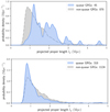 |
Fig. 20. Observed projected proper length PDFs for SDSS-classified quasar and non-quasar giants, obtained through kernel density estimation. We used a Gaussian kernel with σKDE = 75 kpc. For both panels, two-sample Kolmogorov–Smirnov tests yield p < 1‰. However, given the severe impact of selection effects, we could not reject the null hypothesis that quasar giants and non-quasar giants have the same underlying projected proper length distribution. Top: newly discovered (LoTSS DR2) giants with SDSS spectral class labels. Bottom: all known giants with SDSS spectral class labels. |
5. Discussion
5.1. Radio galaxy length definitions
How large are radio galaxies? Despite the simplicity of this question and more than half a century of research on radio galaxies, their intrinsic length distribution has not yet been rigorously characterised. In this work, we have carried out the first precision analysis of the tail of the radio galaxy intrinsic length distribution. Precision analyses tend to raise questions; firstly, whether the studied observable is well defined, and secondly whether one could conceive of more informative observables – that is to say those that make it easier to reveal underlying physical mechanisms. This work’s main observable is the radio galaxy projected proper length; we argue that it is neither well defined nor maximally informative.
5.1.1. The current length definition: survey-dependence
Contemporary research uses a survey-dependent definition for radio galaxy angular lengths, which then makes projected proper lengths survey-dependent too.
The angular length is canonically defined as the largest possible angular separation between two directions for which the RG’s specific intensity function Iν, RG exceeds bν, th: some specified factor of order unity times the image noise σIν. A complication is that not only Iν, RG, but also σIν varies with observing frequency; the latter because of observational factors such as (u,v)-coverage, bandpass, radio-frequency interference (RFI), ionospheric weather, the sky density of bright calibrators and the performance of calibration algorithms. Iν, RG additionally depends on resolution, at least for point sources; σIν additionally depends on resolution and integration time. As a result, both Iν, RG and the concrete value of bν, th used in the angular length definition change from image to image. Each study thus far has therefore implicitly used a different definition for angular length, instead of a shared, absolute one. As the projected proper length follows from combining the angular length with the host redshift, it suffers from the same problem.
Whether the survey-dependence of the current length definition is problematic, depends on the radio galaxy. For archetypal FRII RGs, the angular length is roughly equal to the angular distance between the hotspots. These are an FRII RG’s brightest morphological components, and are thus the first to be picked up by a survey. In contrast, archetypal FRI RGs, which gradually fade with distance from the host, can have significantly larger angular lengths in surveys of higher sensitivity. The giants in the middle-right and bottom-left panel of Fig. 13 are good examples: these radio galaxies were known before the LoTSS DR2, but were not known to be giants; similarly, more sensitive surveys are poised to assign them even larger extents. If we are to move towards precision science, it therefore makes sense – at least for FRI RGs – to more explicitly recognise that the angular and projected proper lengths are functions of the observing frequency νobs and a surface brightness threshold bν, th. If catalogues would explicitly state for what combination (νobs,bν, th) they provide ϕ = ϕ(νobs,bν, th) and lp = lp(νobs,bν, th), it is possible to homogenise a collection of data sets by using universal angular and projected proper length definitions for all RGs22. If two angular lengths have been measured for the same RG, for instance ϕ1 at (νobs, 1,bν, th, 1) and ϕ2 at (νobs, 2,bν, th, 2), then we can estimate ϕ for any desired (νobs,bν, th) through interpolation. For example, the interpolation formula for a symmetric radio galaxy with jets or lobes of constant spectral index α, and with a specific intensity function contribution which fades to zero linearly with angular distance from the host, is
5.1.2. The ideal length definition: physical relevance
Alcyoneus, shown in Fig. 12’s top-right panel, is a 5 Mpc giant whose ageing lobes are revealed for the first time by the LoTSS DR2 (Oei et al. 2022a). Future image sensitivity improvements shall reveal more hitherto unseen, fading lobes around known RGs that formed in the aftermath of earlier AGN activity episodes. Could a large fraction of sufficiently old RGs turn out to be giants, once such sensitivity improvements start providing evidence of earlier and earlier AGN activity episodes?
Up to now, it has been informative to include all visible plasma in the angular length measurement. In future images, some of the visible plasma might be of such low pressure that it has become physically insignificant, in the sense that it does not affect the thermodynamics of the surrounding IGM anymore; we propose to exclude such plasma from a radio galaxy length. Practically, one option is to introduce an absolute threshold: for example to include plasma of pressure P ≥ 10−17 Pa only – this is the pressure of the warm–hot intergalactic medium (WHIM) in the ρBM ∼ 10 ΩBM, 0ρc, 0 and T ∼ 5 × 10⁵ K regime. Another option is to introduce an environment-dependent pressure threshold; this would mean that a cluster RG sees its length measured against a higher pressure threshold than a filament RG, because its plasma becomes thermodynamically irrelevant sooner. A problem with (equipartition or minimum energy) pressure–based length definitions is that pressure is a derived quantity: the specific intensity only determines the product of pressure and line-of-sight length through the lobe.
5.2. Moving beyond line segment projection
In this work, we have adopted a classical approach to treating projection, by modelling radio galaxies as line segments. When a radio galaxy’s inclination angle θ is close to 0° or 180°, this approach predicts that the angular length ϕ and thus the projected proper length lp vanishes. In reality however, because radio galaxy lobes have non-zero volumes, the RV Lp will never tend to zero. Figure 21 illustrates this point through three sources interpreted to be radio galaxies aligned closely with the line of sight. In each case, ϕ remains of arcminute scale.
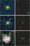 |
Fig. 21. Suspected line-of-sight RGs in the radio and optical. We show 5′×5′ LoTSS DR2 6″ cutouts (left column) and corresponding DESI Legacy Imaging Surveys (g, r, z)-cutouts (right column). Due to its lobes, an RG whose axis aligns closely to the line of sight has a non-zero projected length. From top to bottom row, the SDSS host names are J125027.47+642034.3, J092220.72+560234.9, and J023100.61+032922.1. |
A more realistic approach, outlined in Appendix A.3, moves beyond the simplistic line segment geometry by adding two lobes of radius R to the endpoints of the line segment, whose length is given by RV L. The ratio  , which was unbounded under the classical approach, is now at most
  , where
  . (The classical approach simply is the limit η = 0.) We suggest a recalculation of this work’s theoretical and applied results under this more realistic RG geometry as a direction for future research. To obtain the applied results, one must either fix η as a hyperparameter, or include it as an additional model parameter. We note that even using conservatively low values of η, such as
  , will represent an improvement in realism over η = 0.
5.3. Unmodelled selection effects
In this work, we have modelled both an angular length and a surface brightness selection effect. Several other plausible selection effects have not been included in the forward model, as we have judged each to be of minor importance. However, in unison, they could have a non-negligible influence on the distribution of the observed projected proper GRG length RV Lp, obs | Lp, obs > lp, GRG. Some of their influence might have been absorbed by the parameters of the included selection effects – that is by  , bν, ref, and σref – or, worse still, by ξ.
One of these unmodelled selection effects is that RGs whose axes are oriented almost parallel to the line of sight are more likely to be rejected from a sample than RGs whose axes are closer to the plane of the sky, as the former do not always have a characteristic double-lobe appearance. For instance, perhaps not all readers would regard our identification of the sources in the left column of Fig. 21 as RGs convincing. Nevertheless, as remarked in Sect. 2.11, conditioning Lp, obs | Lp, obs > lp, GRG on inclination angle does not affect its distribution. As a result, this selection effect does not necessitate forward model modifications.
Furthermore, as shown in Sect. 4.4, there is a selection effect at play that favours the selection of quasar giants over non-quasar giants at high redshift, as host galaxies with quasars are more luminous in the optical and therefore have a better chance to be picked up in optical imagery. This selection effect will get less severe once deeper photometric surveys become available.
We encountered three more selection effects during our LoTSS DR2 GRG search. The larger an RG – and especially an FRII RG – becomes, the harder it is for an observer to identify its host galaxy, as an increasing number of plausible host candidates can lie interspersed in the strip of sky between the lobes. The severity of this effect, which diminishes the prevalence of the largest giants in a sample, depends on the balance chosen between avoiding false discoveries and avoiding rejections of true discoveries. Another selection effect runs against RGs in galaxy clusters. Such environments can contain multiple adjacent RGs, making it at times unclear which lobe belongs to which RG. When no confident double-lobe associations can be made, the RGs involved fail to make it into the sample. If galaxy clusters contain primarily smaller giants, this selection effect induces a bias against smaller giants. A final unmodelled bias runs against RGs at the end of their life cycle. Once the AGN stops launching jets for a prolonged period, it becomes hard to identify the host galaxy, which will no longer present as a bright, compact radio source. This effect preferentially deselects larger giants, which are even more likely to approach the end of their life than smaller giants.
5.4. Does the choice of prior matter?
We have taken a conservative approach to constraining the posterior distribution through the prior: we have left tail index ξ and angular length selection half-width  fully unconstrained, and have adopted wide Gaussian priors for reference surface brightness parameters bν, ref and σref, despite measuring them explicitly under assumptions. We provide summary statistics of the posterior in Table 4 and visualise its one- and two-parameter marginals in Fig. 16. Does our choice of prior significantly affect the inferences? To explore this question, we chose a different reasonable prior and compared results. One such prior is the fully uniform prior, which equivalises the posterior and the likelihood function. We provide analogous summary statistics of the likelihood function in Table E.1 and visualise analogous marginals in Fig. E.1. Reassuringly, no statistically significant parameter changes occur. In particular, for zmax = 0.5, ξ = −3.5 ± 0.5 becomes ξ = −3.4 ± 0.5 upon changing to the uniform prior; for zmax = 0.25, ξ = −3.5 ± 0.4 even remains the same. However, given the strong likelihood degeneracy between ξ and bν, ref apparent in Fig. E.1, more stringent priors on bν, ref are able to meaningfully shift ξ’s posterior mean. Such priors shall be appropriate only after studying the surface brightness properties of large radio galaxies – and the associated selection effect – in more detail.
5.5. Cosmological evolution of the GRG length distribution
In this work we have assumed that the parameter ξ, which fully characterises the intrinsic GRG length distribution under the ansatz of Paretianity, remains constant throughout the chosen redshift range [0, zmax]. To test this assumption, we have analysed our LoTSS DR2 GRG sample in Sect. 4 up to both zmax = 0.5 and zmax = 0.25. For zmax = 0.5, we included giants that existed in the last 5 Gyr of the Universe’s history, and found ξ = −3.5 ± 0.5. Meanwhile, for zmax = 0.25, we included giants that existed in the last 3 Gyr of the Universe’s history only, and found the very similar ξ = −3.5 ± 0.4. Thus, our analysis did not produce evidence that ξ evolves over cosmic time. However, given the large error bars, a modest time evolution cannot be excluded. Furthermore, the data sets that underlie these inferences are not disjoint: the 811 giants that inform the lower-maximum-redshift analysis make up 55% of the 1473 giants that inform the higher-maximum-redshift analysis.
Whether a time evolution of ξ is expected is presumably tied to whether giant radio galaxy growth varies with environmental density at a given epoch, because the combined effects of the Universe’s expansion and ongoing large-scale structure formation can similarly change environmental density. Combining our LoTSS DR2 GRG sample with Cosmic Web reconstructions to explore giant growth as a function of environmental density is the topic of a forthcoming work (Oei et al., in prep.). Interestingly, the recent exploration by Lan & Prochaska (2021) that compared the environments of giants and non-giants did not find significant differences.
The most straightforward model extension is to again assume that RG lengths are Pareto distributed with tail index ξ, but now ξ = ξ(z). This function’s first-degree Maclaurin polynomial, which provides the linearisation at the present day, is
One would adopt ξ(z = 0) and  as the parameters of interest, replacing what used to be a constant ξ; the number of model parameters would thus increase by one. However, an attempt to infer the cosmic evolution of ξ appears promising only once the major selection effects are better constrained.
6. Conclusions
In this work, we have performed Bayesian inference on a LoTSS-derived sample of 2060 giant radio galaxy projected proper lengths, using a one-parameter model that assumes a spatially homogeneous, non-evolving population of radio galaxies with stick-like geometry, Pareto-distributed lengths, and isotropic inclination angles. Before fitting to data, we extended the forward model with two selection effects typical of contemporary manual GRG search campaigns. The best-fit survival function tightly reproduces the empirical one, leaving permille-scale absolute residuals. Having quantified the most important selection effects, we estimated the true comoving giant radio galaxy number density in the Local Universe.
-
We developed an analytical model through which statistical questions about radio galaxy (RG) lengths can be rigorously answered. In the current work, we applied this model to giant radio galaxies. We adopted the ansatz that the RG intrinsic proper length L, as measured in three spatial dimensions, is a random variable (RV) with a Pareto Type I distribution (i.e. a simple power-law distribution) characterised by tail index ξ. Next, by assuming that RGs have no preferential orientation with respect to the observer, we derived the distribution of the RG projected proper length Lp. By conditioning, one obtains the version relevant for giants, Lp | Lp > lp, GRG (where we chose lp, GRG := 0.7 Mpc). This RV is again Paretian, with the same tail index ξ. In summary, for giant radio galaxies, projection retains Paretianity. Finally, observers face selection effects; we modelled the observed projected proper length Lp, obs by considering an angular length threshold selection effect and a surface brightness selection effect. The angular length threshold selection effect assumes a linearly increasing angular-length-dependent probability of sample inclusion around a particular pre-defined threshold, meant to emulate manual visual searches that only target RGs of some angular length and above. The surface brightness selection effect assumes that giants are self-similar, and that their lobes have lognormally distributed surface brightnesses which must be above-noise to secure sample inclusion. The GRG observed projected proper length Lp, obs | Lp, obs > lp, GRG again follows through conditioning. We assumed our data to be realisations of this RV.
-
The model also yielded explicit expressions for the (posterior) distribution of L | Lp = lp. This allows one to deproject RGs in a statistical sense, providing the intrinsic proper length given the projected proper length in the limit of negligible selection effects. We also present practical expressions for the mean and variance of L | Lp = lp. To unravel the driving factors that allow some RGs to become giants, most authors search for correlations between host or environmental physical parameters and the GRG projected length. However, if there is a causal chain that connects host or environmental parameters to GRG length, the connection will be to the intrinsic length; the observer’s vantage point does not play a role in the physics. Therefore, the projection effect merely serves as a multiplicative noise source. We suggest that future analyses should recognise the projection effect as such, and correlate host or environmental parameters with the intrinsic, rather than projected, proper length – using statistical deprojection.
-
Through a manual visual search of LoTSS DR2 pipeline products, which are part of the LOFAR’s Northern Sky survey at 144 MHz, we discovered a population of 2060 previously unknown giants. This is the largest single contribution to the literature yet, and increases the community-wide census by a factor 2.6. We present 11 discoveries with lp ≥ 4 Mpc, 53 with 3 ≤ lp < 4 Mpc, 291 with 2 ≤ lp < 3 Mpc, 1215 with 1 ≤ lp < 2 Mpc, and 490 with 0.7 ≤ lp < 1 Mpc. Our study extends the known breadth of the giant radio galaxy phenomenon. Among the findings are both the giant hosted by J081956.41+323537.6 and Alcyoneus (Oei et al. 2022a), at lp = 5.1 Mpc and lp = 5.0 Mpc the projectively largest giants ever found. We discover that multi-Mpc radio galaxies can be generated before redshift 1, despite the Universe’s mean density being an order of magnitude higher, and by spiral galaxies, whose stellar masses are typically an order of magnitude lower than those of ellipticals. We discover giants whose hosts have a record-low stellar mass M⋆ = 4.8 × 10¹⁰ M⊙. We also discover giants whose hosts have a record-high supermassive black hole mass M• ≳ 5 × 10¹⁰ M⊙; interestingly, with lp = 0.8 Mpc, one of these giants is relatively small. We more than double the number of known giants with angular lengths exceeding that of the Moon; one discovery, at 2.2°, is the angularly largest radio galaxy in the Northern Sky and the angularly largest giant overall. Excitingly, our LoTSS DR2 search has been far from exhaustive: many thousands of readily identifiable giants still await discovery in this public data set.
-
Using our LoTSS DR2 GRG sample up to zmax = 0.5, we generated a posterior distribution over ξ and three selection effect parameters. Our model provides an excellent fit to the data, with absolute residuals being on average 2‰. We inferred that the intrinsic proper length distribution of the largest radio galaxies resembles a Pareto distribution with tail index ξ = −3.5 ± 0.5. Our analysis did not yield evidence for an evolving ξ in the last 5 Gyr of cosmic time.
-
The selection effect parameters estimated through the posterior are far from nuisance parameters, as they allowed us to statistically undo the selection effects imprinted on our LoTSS DR2 GRG data. As a result, we could for the first time estimate the true comoving giant radio galaxy number density nGRG in the Local Universe up to zmax. We relied on the crucial assumption that the surface brightness distribution of RGs with intrinsic length lref = 0.7 Mpc at z = 0 and frequency νobs = 144 MHz is unimodal – and lognormal in particular. We furthermore assumed a lobe spectral index α = −1 and self-similar growth. We found nGRG(lp, GRG = 0.7 Mpc, zmax = 0.5) = 5 ± 2(100 Mpc)−3. The implication is that giant radio galaxies are truly rare – not only from a current observational perspective, but also from a cosmological one. Current GRG lobes occupy just a few millionths of the IGM volume. At any given moment in time, most clusters and filaments – the building blocks of modern large-scale structure – do not harbour giants.
Giants embody the most extreme known mechanism by which galaxies can affect the Cosmic Web around them. Whereas this work has explored the geometric properties of giants, a thorough exploration of their Cosmic Web energisation and magnetisation potential is a future frontier. Excitingly, the interactions between giants and the ethereal intergalactic medium may also allow for new constraints on the thermodynamics in filaments.
An object’s size can refer to either its one-, two-, or three-dimensional extent. We therefore consider ‘angular size’ to be ambiguous terminology; we propose that ‘angular length’ better captures one-dimensionality. Naturally, an object’s ‘length’ is understood to be its total one-dimensional extent, so that the qualifier ‘largest’ seems superfluous. We further remark that ‘length’ is synonymous with, but more succinct than, ‘linear size’. In cosmology, one must distinguish between proper and comoving lengths, especially when objects are not gravitationally bound – like GRG lobes. In this work, we consider two types of proper lengths: intrinsic proper lengths and projected proper lengths.
Alcyoneus is the projectively longest giant known to date (Oei et al. 2022a).
For example, the Faint Images of the Radio Sky at Twenty Centimeters (FIRST) survey used the Very Large Array (VLA) in B-configuration, leading it to detect angular scales of at most two arcminutes. By contrast, the largest angular scale of the LoTSS – the survey relevant to this work – is about a degree. (For the 6″ and 20″ resolutions, the shortest baseline is 100 metres; for the 60″ and 90″ resolutions, the shortest baseline is 68 metres.) As virtually all giants are of subdegree angular length, we need not consider this bias in our case.
In this process, we have skipped the enclosed LoTSS DR1 area, which has already been analysed by Dabhade et al. (2020b).
This catalogue, complete up to and including April 2020, contains the giants found in 40 prior publications (for a list, see Dabhade et al. 2020a’s Sect. 1: Introduction), alongside their own discoveries.
At ϕ = 8°, the Southern Sky’s Centaurus A (Cooper et al. 1965) is the radio galaxy with the largest angular length overall (e.g., McKinley et al. 2022); despite this, at lp = 0.48 Mpc, it is not a giant.
We explored two choices for zmax as our model assumes that ξ remains constant between z ∈ [0, zmax]. We further discuss this assumption in Sect. 5.5.
This is also the reason that some giants in Fig. 15 cross their redshift’s dash-dotted curve, which represents fLν = 0.3 and fl = 0.3 only.
In fact, the top panel of Fig. 20 shows expected behaviour for a GRG search campaign with a (fuzzy) angular length threshold selection effect if the unification model is correct. At high redshifts, a GRG must have a larger projected length to pass the angular length threshold than at low redshifts. Thus, sampled high-redshift giants are physically larger than sampled low-redshift giants. Because the fraction of high-redshift quasar giants that is detectable and spectrally classifiable is higher than the fraction of high-redshift non-quasar giants that is detectable and spectrally classifiable, sampled quasar giants will be physically larger than sampled non-quasar giants. To draw this latter conclusion, we must also invoke the fact that, under the unification model, the projected length distributions of quasar and non-quasar giants are the same.
Acknowledgments
M.S.S.L. Oei warmly thanks Frits Sweijen for coding the very useful https://github.com/tikk3r/legacystamps and for tireless ICT advice, and Aleksandar Shulevski for comments that have improved the manuscript. In dear memory of Nicoline. By staying strong despite life’s challenges, you showed what it means to be a giant. M.S.S.L. Oei, R.J. van Weeren, and A. Botteon acknowledge support from the VIDI research programme with project number 639.042.729, which is financed by The Netherlands Organisation for Scientific Research (NWO). A. Drabent acknowledges support by the BMBF Verbundforschung under the grant 05A20STA. The LOFAR is the Low-Frequency Array designed and constructed by ASTRON. It has observing, data processing, and data storage facilities in several countries, which are owned by various parties (each with their own funding sources), and which are collectively operated by the ILT Foundation under a joint scientific policy. The ILT resources have benefited from the following recent major funding sources: CNRS–INSU, Observatoire de Paris and Université d’Orléans, France; BMBF, MIWF–NRW, MPG, Germany; Science Foundation Ireland (SFI), Department of Business, Enterprise and Innovation (DBEI), Ireland; NWO, The Netherlands; the Science and Technology Facilities Council, UK; Ministry of Science and Higher Education, Poland; the Istituto Nazionale di Astrofisica (INAF), Italy. This research made use of the Dutch national e-infrastructure with support of the SURF Cooperative (e-infra 180169) and the LOFAR e-infra group. The Jülich LOFAR Long Term Archive and the German LOFAR network are both coordinated and operated by the Jülich Supercomputing Centre (JSC), and computing resources on the supercomputer JUWELS at JSC were provided by the Gauss Centre for Supercomputing e.V. (grant CHTB00) through the John von Neumann Institute for Computing (NIC). This research made use of the University of Hertfordshire high-performance computing facility and the LOFAR-UK computing facility located at the University of Hertfordshire and supported by STFC [ST/P000096/1], and of the Italian LOFAR IT computing infrastructure supported and operated by INAF, and by the Physics Department of the University of Turin (under an agreement with Consorzio Interuniversitario per la Fisica Spaziale) at the C3S Supercomputing Centre, Italy. Funding for SDSS-III has been provided by the Alfred P. Sloan Foundation, the Participating Institutions, the National Science Foundation, and the U.S. Department of Energy Office of Science. The SDSS-III web site is http://www.sdss3.org/. SDSS-III is managed by the Astrophysical Research Consortium for the Participating Institutions of the SDSS-III Collaboration including the University of Arizona, the Brazilian Participation Group, Brookhaven National Laboratory, Carnegie Mellon University, University of Florida, the French Participation Group, the German Participation Group, Harvard University, the Instituto de Astrofísica de Canarias, the Michigan State/Notre Dame/JINA Participation Group, Johns Hopkins University, Lawrence Berkeley National Laboratory, Max Planck Institute for Astrophysics, Max Planck Institute for Extraterrestrial Physics, New Mexico State University, New York University, Ohio State University, Pennsylvania State University, University of Portsmouth, Princeton University, the Spanish Participation Group, University of Tokyo, University of Utah, Vanderbilt University, University of Virginia, University of Washington, and Yale University. The Pan-STARRS1 Surveys (PS1) and the PS1 public science archive have been made possible through contributions by the Institute for Astronomy, the University of Hawaii, the Pan-STARRS Project Office, the Max-Planck Society and its participating institutes, the Max Planck Institute for Astronomy, Heidelberg and the Max Planck Institute for Extraterrestrial Physics, Garching, The Johns Hopkins University, Durham University, the University of Edinburgh, the Queen’s University Belfast, the Harvard–Smithsonian Center for Astrophysics, the Las Cumbres Observatory Global Telescope Network Incorporated, the National Central University of Taiwan, the Space Telescope Science Institute, the National Aeronautics and Space Administration under Grant No. NNX08AR22G issued through the Planetary Science Division of the NASA Science Mission Directorate, the National Science Foundation Grant No. AST-1238877, the University of Maryland, Eötvös Loránd University (ELTE), the Los Alamos National Laboratory, and the Gordon and Betty Moore Foundation. This work has made use of data from the European Space Agency (ESA) mission Gaia (https://www.cosmos.esa.int/gaia), processed by the Gaia Data Processing and Analysis Consortium (DPAC, https://www.cosmos.esa.int/web/gaia/dpac/consortium). Funding for the DPAC has been provided by national institutions, in particular the institutions participating in the Gaia Multilateral Agreement. The Legacy Surveys consist of three individual and complementary projects: the Dark Energy Camera Legacy Survey (DECaLS; Proposal ID #2014B-0404; PIs: David Schlegel and Arjun Dey), the Beijing–Arizona Sky Survey (BASS; NOAO Prop. ID #2015A-0801; PIs: Zhou Xu and Xiaohui Fan), and the Mayall z-band Legacy Survey (MzLS; Prop. ID #2016A-0453; PI: Arjun Dey). DECaLS, BASS and MzLS together include data obtained, respectively, at the Blanco telescope, Cerro Tololo Inter-American Observatory, NSF’s NOIRLab; the Bok telescope, Steward Observatory, University of Arizona; and the Mayall telescope, Kitt Peak National Observatory, NOIRLab. The Legacy Surveys project is honored to be permitted to conduct astronomical research on Iolkam Du’ag (Kitt Peak), a mountain with particular significance to the Tohono O’odham Nation. NOIRLab is operated by the Association of Universities for Research in Astronomy (AURA) under a cooperative agreement with the National Science Foundation. This project used data obtained with the Dark Energy Camera (DECam), which was constructed by the Dark Energy Survey (DES) collaboration. Funding for the DES Projects has been provided by the U.S. Department of Energy, the U.S. National Science Foundation, the Ministry of Science and Education of Spain, the Science and Technology Facilities Council of the United Kingdom, the Higher Education Funding Council for England, the National Center for Supercomputing Applications at the University of Illinois at Urbana-Champaign, the Kavli Institute of Cosmological Physics at the University of Chicago, Center for Cosmology and Astro-Particle Physics at the Ohio State University, the Mitchell Institute for Fundamental Physics and Astronomy at Texas A&M University, Financiadora de Estudos e Projetos, Fundacao Carlos Chagas Filho de Amparo, Financiadora de Estudos e Projetos, Fundacao Carlos Chagas Filho de Amparo a Pesquisa do Estado do Rio de Janeiro, Conselho Nacional de Desenvolvimento Cientifico e Tecnologico and the Ministerio da Ciencia, Tecnologia e Inovacao, the Deutsche Forschungsgemeinschaft and the Collaborating Institutions in the Dark Energy Survey. The Collaborating Institutions are Argonne National Laboratory, the University of California at Santa Cruz, the University of Cambridge, Centro de Investigaciones Energeticas, Medioambientales y Tecnologicas-Madrid, the University of Chicago, University College London, the DES-Brazil Consortium, the University of Edinburgh, the Eidgenössische Technische Hochschule (ETH) Zürich, Fermi National Accelerator Laboratory, the University of Illinois at Urbana-Champaign, the Institut de Ciencies de l’Espai (IEEC/CSIC), the Institut de Fisica d’Altes Energies, Lawrence Berkeley National Laboratory, the Ludwig Maximilians Universität München and the associated Excellence Cluster Universe, the University of Michigan, NSF’s NOIRLab, the University of Nottingham, the Ohio State University, the University of Pennsylvania, the University of Portsmouth, SLAC National Accelerator Laboratory, Stanford University, the University of Sussex, and Texas A&M University. BASS is a key project of the Telescope Access Program (TAP), which has been funded by the National Astronomical Observatories of China, the Chinese Academy of Sciences (the Strategic Priority Research Program “The Emergence of Cosmological Structures” Grant # XDB09000000), and the Special Fund for Astronomy from the Ministry of Finance. The BASS is also supported by the External Cooperation Program of Chinese Academy of Sciences (Grant # 114A11KYSB20160057), and Chinese National Natural Science Foundation (Grant # 11433005). The Legacy Survey team makes use of data products from the Near-Earth Object Wide-field Infrared Survey Explorer (NEOWISE), which is a project of the Jet Propulsion Laboratory/California Institute of Technology. NEOWISE is funded by the National Aeronautics and Space Administration. The Legacy Surveys imaging of the DESI footprint is supported by the Director, Office of Science, Office of High Energy Physics of the U.S. Department of Energy under Contract No. DE-AC02-05CH1123, by the National Energy Research Scientific Computing Center, a DOE Office of Science User Facility under the same contract; and by the U.S. National Science Foundation, Division of Astronomical Sciences under Contract No. AST-0950945 to NOAO.
References
- Ahn, C. P., Alexandroff, R., Allende Prieto, C., et al. 2012, ApJS, 203, 21 [Google Scholar]
- Alam, S., Albareti, F. D., Prieto, C. A., et al. 2015, ApJS, 219, 12 [NASA ADS] [CrossRef] [Google Scholar]
- Amirkhanyan, V. R. 2016, Astrophys. Bull., 71, 384 [NASA ADS] [CrossRef] [Google Scholar]
- Andernach, H., Jiménez-Andrade, E. F., & Willis, A. G. 2021, Galaxies, 9, 99 [NASA ADS] [CrossRef] [Google Scholar]
- Bagchi, J., Vivek, M., Vikram, V., et al. 2014, ApJ, 788, 174 [NASA ADS] [CrossRef] [Google Scholar]
- Bassani, L., Ursini, F., Malizia, A., et al. 2021, MNRAS, 500, 3111 [Google Scholar]
- Beckmann, R. S., Devriendt, J., Slyz, A., et al. 2017, MNRAS, 472, 949 [NASA ADS] [CrossRef] [Google Scholar]
- Blandford, R. D., & Rees, M. J. 1974, MNRAS, 169, 395 [NASA ADS] [CrossRef] [Google Scholar]
- Bloom, J. S., Frail, D. A., & Sari, R. 2001, AJ, 121, 2879 [NASA ADS] [CrossRef] [Google Scholar]
- Bonnarel, F., Fernique, P., Bienaymé, O., et al. 2000, A&AS, 143, 33 [NASA ADS] [CrossRef] [EDP Sciences] [Google Scholar]
- Brüggen, M., Reiprich, T. H., Bulbul, E., et al. 2021, A&A, 647, A3 [NASA ADS] [CrossRef] [EDP Sciences] [Google Scholar]
- Chambers, K. C., Magnier, E. A., Metcalfe, N., et al. 2016, ArXiv e-prints [arXiv:1612.05560] [Google Scholar]
- Chang, Y.-Y., van der Wel, A., da Cunha, E., & Rix, H.-W. 2015, ApJS, 219, 8 [Google Scholar]
- Condon, J. J., Cotton, W. D., Greisen, E. W., et al. 1998, AJ, 115, 1693 [Google Scholar]
- Cooper, B. F. C., Price, R. M., & Cole, D. J. 1965, Aust. J. Phys., 18, 589 [NASA ADS] [Google Scholar]
- Croton, D. J., Springel, V., White, S. D. M., et al. 2006, MNRAS, 365, 11 [Google Scholar]
- Dabhade, P., Gaikwad, M., Bagchi, J., et al. 2017, MNRAS, 469, 2886 [NASA ADS] [CrossRef] [Google Scholar]
- Dabhade, P., Mahato, M., Bagchi, J., et al. 2020a, A&A, 642, A153 [NASA ADS] [CrossRef] [EDP Sciences] [Google Scholar]
- Dabhade, P., Röttgering, H. J. A., Bagchi, J., et al. 2020b, A&A, 635, A5 [NASA ADS] [CrossRef] [EDP Sciences] [Google Scholar]
- Dálya, G., Galgóczi, G., Dobos, L., et al. 2018, MNRAS, 479, 2374 [Google Scholar]
- Delhaize, J., Heywood, I., Prescott, M., et al. 2021, MNRAS, 501, 3833 [Google Scholar]
- Dey, A., Schlegel, D. J., Lang, D., et al. 2019, AJ, 157, 168 [Google Scholar]
- Di Matteo, T., Springel, V., & Hernquist, L. 2005, Nature, 433, 604 [NASA ADS] [CrossRef] [Google Scholar]
- Fabian, A. C., Nulsen, P. E. J., & Canizares, C. R. 1984, Nature, 310, 733 [NASA ADS] [CrossRef] [Google Scholar]
- Forero-Romero, J. E., Hoffman, Y., Gottlöber, S., Klypin, A., & Yepes, G. 2009, MNRAS, 396, 1815 [Google Scholar]
- Gaia Collaboration (Prusti, T., et al.) 2016, A&A, 595, A1 [NASA ADS] [CrossRef] [EDP Sciences] [Google Scholar]
- Gaia Collaboration (Brown, A. G. A., et al.) 2021, A&A, 649, A1 [NASA ADS] [CrossRef] [EDP Sciences] [Google Scholar]
- Galvin, T. J., Huynh, M. T., Norris, R. P., et al. 2020, MNRAS, 497, 2730 [NASA ADS] [CrossRef] [Google Scholar]
- Gürkan, G., Prandoni, I., O’Brien, A., et al. 2022, MNRAS, 512, 6104 [CrossRef] [Google Scholar]
- Hardcastle, M. J. 2018, MNRAS, 475, 2768 [Google Scholar]
- Hardcastle, M. J., & Croston, J. H. 2020, New A Rev., 88, 101539 [NASA ADS] [CrossRef] [Google Scholar]
- Hart, R. E., Bamford, S. P., Willett, K. W., et al. 2016, MNRAS, 461, 3663 [NASA ADS] [CrossRef] [Google Scholar]
- Ishwara-Chandra, C. H., Taylor, A. R., Green, D. A., et al. 2020, MNRAS, 497, 5383 [Google Scholar]
- Jansen, R. A., Franx, M., Fabricant, D., & Caldwell, N. 2000, ApJS, 126, 271 [NASA ADS] [CrossRef] [Google Scholar]
- Jasche, J., & Lavaux, G. 2019, A&A, 625, A64 [NASA ADS] [CrossRef] [EDP Sciences] [Google Scholar]
- Jasche, J., & Wandelt, B. D. 2013, MNRAS, 432, 894 [Google Scholar]
- Jasche, J., Leclercq, F., & Wandelt, B. D. 2015, JCAP, 2015, 036 [Google Scholar]
- King, A. 2016, MNRAS, 456, L109 [CrossRef] [Google Scholar]
- Kirk, J. G., & Schneider, P. 1987, ApJ, 315, 425 [NASA ADS] [CrossRef] [Google Scholar]
- Kormendy, J., & Ho, L. C. 2013, ARA&A, 51, 511 [Google Scholar]
- Krause, M., Alexander, P., Riley, J., & Hopton, D. 2012, MNRAS, 427, 3196 [NASA ADS] [CrossRef] [Google Scholar]
- Kroupa, P. 2001, MNRAS, 322, 231 [NASA ADS] [CrossRef] [Google Scholar]
- Kuźmicz, A., & Jamrozy, M. 2021, ApJS, 253, 25 [CrossRef] [Google Scholar]
- Lan, T.-W., & Prochaska, J. X. 2021, MNRAS, 502, 5104 [Google Scholar]
- Mahato, M., Dabhade, P., Saikia, D. J., et al. 2022, A&A, 660, A59 [NASA ADS] [CrossRef] [EDP Sciences] [Google Scholar]
- Malevergne, Y., Pisarenko, V., & Sornette, D. 2011, Phys. Rev. E, 83, 036111 [Google Scholar]
- Masini, A., Celotti, A., Grandi, P., Moravec, E., & Williams, W. L. 2021, A&A, 650, A51 [NASA ADS] [CrossRef] [EDP Sciences] [Google Scholar]
- McKinley, B., Tingay, S. J., Gaspari, M., et al. 2022, Nat. Astron., 6, 109 [Google Scholar]
- McNamara, B. R., & Nulsen, P. E. 2012, New J. Phys., 14, 055023 [NASA ADS] [CrossRef] [Google Scholar]
- Mostert, R. I. J., Duncan, K. J., Röttgering, H. J. A., et al. 2021, A&A, 645, A89 [NASA ADS] [CrossRef] [EDP Sciences] [Google Scholar]
- Oei, M. S. S. L., van Weeren, R. J., Hardcastle, M. J., et al. 2022a, A&A, 660, A2 [NASA ADS] [CrossRef] [EDP Sciences] [Google Scholar]
- Oei, M. S. S. L., van Weeren, R. J., Vazza, F., et al. 2022b, A&A, 662, A87 [NASA ADS] [CrossRef] [EDP Sciences] [Google Scholar]
- Oei, M. S. S. L., van Weeren, R. J., Hardcastle, M. J., et al. 2023, MNRAS, 518, 240 [Google Scholar]
- Planck Collaboration VI. 2020, A&A, 641, A6 [NASA ADS] [CrossRef] [EDP Sciences] [Google Scholar]
- Proctor, D. D. 2016, ApJS, 224, 18 [NASA ADS] [CrossRef] [Google Scholar]
- Ringermacher, H. I., & Mead, L. R. 2009, MNRAS, 397, 164 [NASA ADS] [CrossRef] [Google Scholar]
- Rybicki, G. B., & Lightman, A. P. 1986, Radiative Processes in Astrophysics (Wiley-VCH), 400 [Google Scholar]
- Salim, S., Boquien, M., & Lee, J. C. 2018, ApJ, 859, 11 [Google Scholar]
- Shimwell, T. W., Röttgering, H. J. A., Best, P. N., et al. 2017, A&A, 598, A104 [NASA ADS] [CrossRef] [EDP Sciences] [Google Scholar]
- Shimwell, T. W., Tasse, C., Hardcastle, M. J., et al. 2019, A&A, 622, A1 [NASA ADS] [CrossRef] [EDP Sciences] [Google Scholar]
- Shimwell, T. W., Hardcastle, M. J., Tasse, C., et al. 2022, A&A, 659, A1 [NASA ADS] [CrossRef] [EDP Sciences] [Google Scholar]
- Simonte, M., Andernach, H., Brüggen, M., et al. 2022, MNRAS, 515, 2032 [CrossRef] [Google Scholar]
- Solovyov, D. I., & Verkhodanov, O. V. 2011, Astrophys. Bull., 66, 416 [NASA ADS] [CrossRef] [Google Scholar]
- Solovyov, D. I., & Verkhodanov, O. V. 2014, Astrophys. Bull., 69, 141 [NASA ADS] [CrossRef] [Google Scholar]
- Tang, H., Scaife, A. M. M., Wong, O. I., et al. 2020, MNRAS, 499, 68 [Google Scholar]
- Turner, R. J., & Shabala, S. S. 2015, ApJ, 806, 59 [Google Scholar]
- van Haarlem, M. P., Wise, M. W., Gunst, A. W., et al. 2013, A&A, 556, A2 [NASA ADS] [CrossRef] [EDP Sciences] [Google Scholar]
- Vazza, F., Brüggen, M., Gheller, C., et al. 2017, CQG, 34, 234001 [NASA ADS] [CrossRef] [Google Scholar]
- Wen, Z. L., Han, J. L., & Liu, F. S. 2012, ApJS, 199, 34 [Google Scholar]
- Yang, H. Y. K., Gaspari, M., & Marlow, C. 2019, ApJ, 871, 6 [CrossRef] [Google Scholar]
- Zheng, H., Tegmark, M., Dillon, J. S., et al. 2017, MNRAS, 464, 3486 [NASA ADS] [CrossRef] [Google Scholar]
- Zou, H., Sui, J., Xue, S., et al. 2022, Res. Astron. Astrophys., 22, 065001 [Google Scholar]
Appendix A: Framework derivations and details
A.1. Intrinsic proper length
Let fL : ℝ → ℝ≥0 be the PDF of the distribution of intrinsic (i.e. 3D) proper (i.e. not comoving) radio galaxy lengths L. We assume that fL follows a power law between lmin and lmax:
Then, when ξ ≠ −1,
This equation provides the normalisation factor fL(lref) given lmin, lmax, ξ and an arbitrary choice for lref ≠ 0.
When lmax = ∞, L has a Pareto Type I distribution and we must have ξ < −1 for the integrals of Eq. A.2 to converge. Throughout the remaining analysis, for the sake of simplicity, we assume lmax = ∞ and ξ < −1 and choose lref = lmin. Then  . The corresponding CDF is
In reality, radio galaxies cannot become arbitrarily long (Hardcastle 2018): at some distance from the host, all energy carried by the jets will have been radiated away, used to perform work on the IGM, transferred to CMB photons through inverse Compton scattering, or converted into heat. However, at the moment of writing, the implied maximum length lmax remains ill-constrained. As we see throughout Appendix A, a major advantage of simple model assumptions is that explicit and thus insightful analytic expressions can be derived. Such easy-to-evaluate expressions complement the results of expensive numerical simulations, which aim to maximise realism; our aim to maximise insight is best served by setting lmax = ∞. From Eq. A.3, we see that for lmin = 0.7 Mpc and ξ = −3.5, the tail of the intrinsic proper length distribution (l > 5 Mpc) contains less than 1% of probability. Thus, for most framework applications, our choice lmax = ∞ is unproblematic — except when higher powers of L are involved. For example, the volume-filling fraction calculations of Appendix A.10 necessitate considering L3; for realistic ξ, results exist only for finite lmax.
Upon relabelling ξ → −α − 1, lmin → k, L → X and l → x, one obtains the literature’s most common form of the Pareto Type I PDF:
A.2. Projected proper length
A.2.1. Distribution for RGs
Let fLp : ℝ → ℝ≥0 be the PDF of the distribution of projected proper radio galaxy lengths. The PDF fLp follows from the associated CDF FLp : ℝ → [0, 1] through differentiation; FLp and fL relate through
We note that FLp(lp) vanishes for lp ≤ 0: fL(l) vanishes when l is negative, whilst  vanishes when l is positive. Clearly, the interesting case is lp > 0. We can differentiate between two cases: lp ≤ lmin, and lp > lmin. In the first case, considering that fL has support from lmin onwards only, we have
  , and
, and
In the second case, we split up the integral in two:
In summary,
Through differentiation,
where
Significantly, for lp > lmin, the projected length distribution follows a power law in lp with the same exponent as the power law for the intrinsic length distribution:  (just as fL ∝ lξ).23 We compare fL and fLp in Fig. 1.
A.2.2. Distribution for giants
To derive the projected length distribution for giants, we consider the distribution of the conditioned RV Lp | Lp > lp, GRG:
For lp > lp, GRG, this reduces to
Furthermore assuming lp, GRG > lmin, we twice use the bottom expression of Eq. A.8 to obtain the final CDF expression. As before, the corresponding PDF follows through differentation. We find
Thus, the associated survival function is
The mean projected proper length of giants follows from the PDF by direct computation:
A.3. Deprojection factor
Consider a radio galaxy (RG) with a projected proper length lp. Let the inclination angle θ denote the angle between the RG’s central axis and the line of sight. The RG’s inclination angle, projected proper length and intrinsic proper length l relate via lp = l sin θ. Switching to random variable (RV) notation by using capital letters, the intrinsic proper length (which is the most physically relevant quantity) follows from the projected proper length (which can be measured) and the inclination angle (which is typically unknown), according to
A.3.1. Without lobes
Calling the deprojection factor D := (sin Θ)−1, we now calculate the distribution of D for ![$ f_\Theta\left(\theta\right) = \frac{1}{2}\sin{\theta}; \theta \in [0, \pi] $](/articles/aa/full_html/2023/04/aa43572-22/aa43572-22-eq116.gif) . The result is a continuous univariate distribution without parameters supported on the semi-infinite interval (1,∞). Let FD : ℝ → [0, 1] be the cumulative density function (CDF) of D. Then, for d > 1,
. The result is a continuous univariate distribution without parameters supported on the semi-infinite interval (1,∞). Let FD : ℝ → [0, 1] be the cumulative density function (CDF) of D. Then, for d > 1,
Meanwhile, FD(d) = 0 for d ≤ 1. The quantile function ![$ F_D^{-1}\!: [0, 1] \to [1, \infty) $](/articles/aa/full_html/2023/04/aa43572-22/aa43572-22-eq118.gif) follows from solving FD(d) = p for d:
follows from solving FD(d) = p for d:
Thus, the minimum factor is  , the median
  ,
,  ,
,  , and factors can grow arbitrarily large:
  as p → 1. We conclude that half of all RGs have an intrinsic proper length more than
  their projected proper length.
By differentiating FD to d we obtain fD : ℝ → ℝ≥0, the probability density function (PDF) of D:
The mean of D is  ; the variance of D is undefined, as the corresponding integral diverges. Because fD(d) has no maximum, the mode is undefined too. The PDF and CDF of D are shown in the upper left and right panels of Fig. A.1, respectively.
 |
Fig. A.1. PDFs (left column) and CDFs (right column) of the deprojection factor RV D. These functions quantify how much longer RGs are than their projected lengths suggest. Top row: model without lobes. Of the three canonical measures of central tendency, only the median and mean exist (and equal |
A.3.2. With lobes
The simplest model that includes a pair of lobes approximates them as spheres of radius R, whose centres are connected by a line segment of length L. Regardless of the viewing angle, the spheres retain their size, in contrast to the line segment connecting them. Calling  , we have
Again assuming ![$ f_\Theta\left(\theta\right) = \frac{1}{2}\sin{\theta}; \theta \in [0, \pi] $](/articles/aa/full_html/2023/04/aa43572-22/aa43572-22-eq132.gif) , we repeat the derivation and find
, we repeat the derivation and find
The quantile function becomes
The minimum factor remains  , but a maximum factor now exists:
  . The median of D is
which tends to  for η → 0 (as before), and to 1 for η → ∞: projection ceases to be an appreciable effect when the lobes are much larger than the line segment connecting their centres. If η ≠ 0, D has finite support, and thus the mean, variance and higher moments exist. The n-th non-central moment is
where
In particular,
The expectation value of D is
The variance of D follows from combining
and the identity 𝕍[D] = 𝔼[D2] − 𝔼2[D]. The mode remains undefined. For typical values of η, we show the PDF and CDF of D in the bottom left and right panels of Fig. A.1, respectively. Figure A.2 shows the median, mean and standard deviation of D as a function of η.
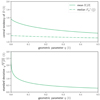 |
Fig. A.2. Summary statistics for the deprojection factor RV D under the spherical lobe model. Top: the η-dependency of two measures of central tendency of D. For η = 0, the mean |
A.4. Intrinsic proper length posterior and its moments
Our next objective is to find the posterior PDF fL|Lp = lp(l) through Bayes’ theorem:
Our line of attack will be to first calculate the likelihood CDF FLp|L = l(lp), and then through differentiation the likelihood PDF fLp|L = l(lp). Of course, we always consider l > 0, and
where we have invoked Eq. A.17 and the fact that fΘ(θ) is symmetric in  for the case 0 < lp < l. Concretising this case further yields
Through differentiation,
Having found the likelihood, the posterior PDF follows directly through Bayes’ theorem and the PDFs computed hitherto.
In concreto, when 0 < lp ≤ lmin,
whereas for lp > lmin,
We note that in both cases, for l ≫ lp,  : the posterior probability density follows a power law in l with exponent ξ − 2.
For lp ≤ lmin, the posterior mean is
The posterior variance 𝕍[L | Lp=lp] follows from considering the second non-central moment:
so that
For lp > lmin,
Proceeding analogously,
so that
In this case, both the mean and standard deviation of L | Lp = lp are proportional to lp. In the table below, we list the mean and standard deviation in multiples of lp for several values of ξ. Since we assume ξ < −1, the mean and variance are guaranteed to exist. The existence of higher-order moments is ξ-dependent; in concreto, the highest defined order is ⌈ − ξ⌉.
We prove that Lp and D are not independent by contradiction. If we assume that Lp and D are independent, then 𝔼[LpD]=𝔼[Lp]𝔼[D], or 𝔼[L]=𝔼[L]𝔼[sin Θ]𝔼[D] by the independence of L and sin Θ. In other words, if Lp and D are independent, then 1 = 𝔼[sin Θ]𝔼[D]. However, ![$ \mathbb{E}[\sin{\Theta}] = \frac{\pi}{4} $](/articles/aa/full_html/2023/04/aa43572-22/aa43572-22-eq162.gif) and
and ![$ \mathbb{E}[D] = \frac{\pi}{2} $](/articles/aa/full_html/2023/04/aa43572-22/aa43572-22-eq163.gif) ; because
; because  , the initial assertion must be wrong.
A.5. GRG inclination angle
We derive the inclination angle distribution for giants. The probability that a GRG has inclination angle θ is
where we make use of the fact that the numerator’s joint probability factorises because L and Θ are independent RVs. We thus find
Under the Paretian assumption for L, we have
A.6. GRG angular length
The GRG angular length RV Φ | Lp > lp, GRG relates to the GRG projected proper length RV Lp | Lp > lp, GRG and the comoving distance RV R as
The model predicts the distribution of GRG angular lengths in the Local Universe up to comoving distance rmax. If the GRG number density is constant in the Local Universe,
Because GRG life cycles are shorter than the age of the Universe, Lp | Lp > lp, GRG and R are independent RVs. In a non-expanding universe, z(R) = 0, and the distribution of Φ | Lp > lp, GRG can be calculated analytically. From a well-known ratio distribution identity,
The integrand is non-zero only when ϕr ≥ lp, GRG, suggesting a lower integration limit of  . The integral vanishes altogether when
  . Calling
  , we have fΦ | Lp > lp, GRG(ϕ) = 0 for ϕ ≤ ϕGRG. For ϕ > ϕGRG,
where we assume ξ ≠ −4. This PDF depends on ξ, lp, GRG, and rmax only. The CDF follows from direct integration:
just as the mean:
which exists only for ξ < −2. By solving
for the GRG angular length mode ϕmode, we find
There is no explicit expression for the associated median.
For a general non-Euclidean universe, no simple analytic form for the GRG angular length PDF appears to exist. We find an approximation valid at low redshifts by considering the Maclaurin polynomial of degree 1 for z(r), the relation between comoving distance and cosmological redshift. One finds  . As a result, for the Local Universe, Eq. 14 becomes
where we use that the Hubble distance  . From a well-known inverse distribution identity,
so that
Combining a well-known product distribution identity with the fact that Lp | Lp > lp, GRG and  are independent RVs, we find
when  . When
  , fΦ | Lp > lp, GRG(ϕ) = 0. It is easy to verify that in the Euclidean limit,
  , this expression reduces to that of Eq. A.50.
A.7. Maximum likelihood estimation of the tail index
How can we estimate ξ from a sample of N giants? Let ξMLE be the maximum likelihood estimate (MLE) of ξ. This RV is a function of N IID RVs {Lp, 1, ..., Lp, N}∼Lp | Lp > lp, GRG. Define the following likelihood and log-likelihood functions:
We note the necessity to include a factor  in the definition of the log-likelihood to avoid a dimensionality error. The second derivative of
  to ξ is
Thus, if there exists a solution to the equation  , it must correspond to a global maximum of the likelihood and log-likelihood functions:
A.8. Observed projected proper length
A.8.1. General considerations
The model can be extended to incorporate observational selection effects. The relevant effects to consider vary from RG search campaign to RG search campaign, although some formulae apply in all cases. We derive these here.
To keep our extensions simple, we assume that the survey sensitivity is sufficient to detect RGs up to some redshift zmax only. In addition we assume that the projected proper length distribution does not evolve between z = zmax and z = 0. We let pobs(lp, z) denote the probability that an RG of projected proper length lp at cosmological redshift z is detected during the campaign. Also, r is the radial comoving distance and n is the total RG number density, counting the intrinsic number of RGs (irrespective of length) per unit of comoving volume. The observed number of RGs with projected proper length between lp and lp + dlp throughout a survey covering a solid angle Ω is dNLp, obs(lp,Ω), where
The total number of RGs with projected proper length between lp and lp + dlp throughout a survey with solid angle Ω is dNLp(lp,Ω), where
We define the completeness C(lp, zmax) to be
The completeness only depends on the function pobs(lp, z) and our choice of zmax.
Let the RV 𝒪 denote whether an RG picked at random within z < zmax is detected during the search campaign. We have 𝒪 ∼ Bernoulli(C(Lp,zmax)); the parameter that determines the distribution of 𝒪 is itself an RV. It immediately follows that ℙ(𝒪 = 1 | Lp=lp) = C(lp, zmax).
If Lp would be discrete,
Let Lp, obs be the observed projected proper length RV; that is Lp, obs := Lp | 𝒪 = 1. Its PDF is given by the continuous analogon of the preceding equation:
Obviously,  . The CDF FLp, obs|Lp, obs > lp, GRG(lp) follows from an analogon of Eq. A.12.
We note that multiplying pobs(lp, z) with an lp- and z-independent factor changes C(lp, zmax) by the same factor, but leaves fLp, obs unaltered.
A.8.2. Fuzzy angular length threshold
Here we illustrate a simple extension. When performing visual searches for GRG candidates, a natural criterion is to only inspect sources with an angular length that is larger than some threshold. Researchers determine the threshold based on the amount of time available to them: lower thresholds will lead to more complete samples, but will take more time to collect. For humans, it is hard to estimate a source’s angular length precisely by eye; as a result, some of the GRG candidates included in the project’s GRG candidate catalogue will be sources with an angular length below the threshold, whilst others will be sources with an angular length above the threshold. We idealise this situation by asserting that sources with angular length ϕmin or below are included in the catalogue with probability 0 (i.e. never), and that sources with an angular length ϕmax or above are included in the catalogue with probability 1 (i.e. always). We assume a linear increase in probability as a function of ϕ for intermediate angular lengths: a source with angular length ϕmin < ϕ < ϕmax is included in the catalogue with probability
In a flat Friedmann–Lemaître–Robertson–Walker (FLRW) universe, the angular length of an RG with projected proper length lp at cosmological redshift z is
A.8.3. Surface brightness limitations
Fanaroff–Riley class II If the surface brightness Bν of the lobes is proportional to some negative power ζ of the GRG’s proper length L, that is
then Bν is Pareto distributed — just like L:
If RGs are self-similar in shape, then their lobe volumes are proportional to L3. RGs appear to retain constant lobe luminosity density over most of their lifetime, so that their lobe monochromatic emission coefficients (Rybicki & Lightman 1986) are proportional to L−3. As line-of-sight lengths through the lobes are proportional to L, surface brightness is proportional to L−2. These arguments thus suggest ζ = −2.
It is a poor approximation to assume that all giants of proper length lref have the same surface brightness bν, ref: observations suggest a variability of several orders of magnitude. A better description is
where S is a lognormal RV whose median is 1. The PDF of S is then determined by parameter σref:
The surface brightness CDF and PDF now become
We note that Bν is not exactly Pareto distributed anymore.
In a relativistic rather than Euclidean universe, surface brightness is not constant with distance. To describe RGs beyond z = 0, we introduce a final model refinement:
where the RV Z denotes cosmological redshift and α is the spectral index of the lobes. We interpret bν, ref ⋅ S as the (lognormally distributed) lobe surface brightness for RGs of intrinsic proper length lref at z = 0. In this case, the CDF and PDF of Bν are most easily determined through sampling. To sample Z, we can first sample the comoving distance RV R instead, and subsequently use Z = z𝔐(R). We stress that this conversion depends on cosmological parameters 𝔐.
To forward model a survey’s surface brightness selection effect, we must compute
where bν, th > 0 is the surface brightness threshold. Typically, bν, th is comparable to the survey’s RMS noise. What is FBν | Lp = lp, Z = z(b)? In the simplest case, devoid of S- and Z-dependence,
where
Therefore,
In the most refined case, for b > 0,
where
The minimum value of S for which an RG of projected length lp at redshift z is detectable, is  . For brevity, we simply write smin instead. We find
The following approximation might facilitate the numerical evaluation of this integral. We note that for s ≫ smin, the square root factor in the integral approaches 1. Now split up the original integral in two parts, where η governs the approximation’s accuracy:
where we substitute numerically integrating to infinity for an evaluation of the CDF of the lognormally distributed RV S. The approximation error is bounded from above:
Let us assume ζ = −2. For η = 100, the approximation error is at most 0.005, and for η = 1000, the approximation error is at most 0.0005.
Fanaroff–Riley class I The simplest correction in which FRI RGs retain a well-defined notion of length assumes a linearly decreasing surface brightness, from some value bν(0) at the core to zero at the RG’s two endpoints. For a symmetric FRI RG, the surface brightness profile along one of the jets is bν : ℝ≥0 → ℝ≥0, and depends on the projected proper distance from the core rp as
Now we consider an FRI GRG, whose projected proper length lp > lp, GRG would only be observed in full in the absence of noise. In actual observations, this GRG is detected as a GRG if and only if
Under our assumption of a linear surface brightness profile, the mean surface brightness along the jet axis  . As this must be half of the surface brightness at the core,
Combining Eqs. A.87 and A.88, we find that the GRG is detected as such if
Now regarding ⟨bν⟩ as an RV and recognising that it might behave exactly as in Eq. A.76, we find that the surface brightness selection effect for FRI giants may be modelled as
We see that the full formulaic structure of pobs(lp, z) is the same for FRI and FRII giants, except that for FRI giants a change
is necessary. There is no change for lp = 2lp, GRG.
A.9. GRG number density
A statistic of major interest is the number density of giants in the contemporary Universe. Let nGRG be the comoving GRG number density, so that
After invoking Eq. A.63 and isolating n, we obtain
Combining Eqs. A.8, A.9, A.92 and A.94 for lp, GRG > lmin, we arrive at
From observations, we know Ω and can — for a given zmax — simply count NGRG, obs(Ω,zmax). Moreover, we can fit ξ and the parameters that occur in pobs(lp, z) (e.g.  , bν, ref, and σref) to the ECDF of Lp, obs | Lp, obs > lp, GRG. We note that nGRG does not depend on lmin, which drops out through the division. However, nGRG does depend on cosmological parameters through the relation between cosmological redshift z and radial comoving distance r.
A.10. GRG lobe volume-filling fraction
Assuming self-similar growth, the combined proper volume V of an RG’s lobes and its intrinsic proper length l obey V ∝ l3. The constant of proportionality varies per RG and depends on the shape of the lobes; we treat it as an RV  . Then the proper VFF of GRG lobes VFFGRG(z) = VFFGRG(z = 0)⋅(1 + z)3, where
Assuming that RGs grow self-similarly, so that shape does not reveal length, Υ and L3 are conditionally independent given Lp > lp, GRG: Υ ⫫ L3 | Lp > lp, GRG. As a result,
To obtain this last line, we once more exploit self-similarity: Υ | (Lp > lp, GRG) = Υ. We can approximate 𝔼[Υ] by taking the mean of some  deduced from observations. A technical complication arises from the fact that 𝔼[L3 | Lp > lp, GRG] does not exist for ξ ≥ −4 under our model. This is an artefact of the Pareto distribution assumption for L, which unrealistically features support over an infinitely long part of the real line: {l ∈ ℝ | l > lmin}. This causes the expectation value integral to diverge for ξ ≥ −4. An approximation to VFFGRG(z = 0) that works for all ξ is the lower bound
which follows from Jensen’s inequality. Here
Alternative approximation formulae, which use  , are
, are
and
where
is the median of the cubed projected proper length for giants. An advantage of these latter expressions is that there are more data available to estimate 𝔼[Υp] than there are to estimate 𝔼[Υ].
A.10. Unification model constraints from quasar and non-quasar giants
The quasar GRG probability pQ is
Now using Eqs. A.3 and A.8 and  over the domain of integration,
A.11. Extreme giants in a sample
An interesting feature of the model is its ability to predict the occurrence of giants with extreme projected proper lengths in a GRG sample of, say, size N. Now consider some lp > lp, GRG — what is the probability p> lp that an observed GRG will have a projected proper length exceeding lp? Proceeding as in the derivation of Eq. A.12, we find
In the absence of selection effects, p> lp(lp) is given by Eq. A.15. The number of giants with extreme projected proper lengths N> lp ∼ Binom(N, p> lp(lp)).
Interesting questions can be answered readily. For example, the probability that the sample contains at least one GRG with projected proper length lp or larger, is
Appendix B: Additional images
In this appendix, as in Fig. 12, we show newly discovered giants. These cover the projected length range lp ∈ [0.7 Mpc, 4 Mpc).
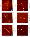 |
Fig. B.1. Details of the LoTSS DR2–estimated specific intensity function |
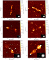 |
Fig. B.2. Details of the LoTSS DR2–estimated specific intensity function |
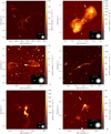 |
Fig. B.3. Details of the LoTSS DR2–estimated specific intensity function |
Appendix C: Stellar and supermassive black hole masses
In Fig. C.1, we present the SDSS-derived relations between host stellar mass and projected proper length, and between host supermassive black hole mass and projected proper length, for all giants in our final catalogue. We obtained the data as in Section 3.7 of Oei et al. (2022a).
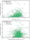 |
Fig. C.1. Observed relations between host stellar mass M⋆ and GRG projected length lp(top) and between host SMBH mass M• and GRG projected length lp(bottom). Our LoTSS DR2 sample confirms that luminous giants typically have M⋆ ∈ 1011–1012 M⊙ and M• ∈ 108–1010 M⊙. The sample effects an almost fivefold increase in the number of giants with SDSS-derived host stellar masses and SMBH masses. We do not show or count giants for which only a nearest host candidate could be determined. |
Appendix D: Surface brightness prior
Consider a radio galaxy at cosmological redshift z of intrinsic proper length l bounded by spherical lobes of radius R and spectral index α. If a fraction fl of the radio galaxy’s central axis lies within the lobes, then
If a fraction fLν of the radio galaxy’s total luminosity density Lν comes from the lobes, then the monochromatic emission coefficient
where the lobe volume  . A formula of practical value features projected proper length lp instead of l. Given the approximate nature of our approach, we therefore simply assume l ≈ 𝔼[D](η(fl)) ⋅ lp, with the deprojection factor expectation 𝔼[D] given in Eq. A.29;
  . The maximum surface brightness of the lobes as seen by an observer is
valid for the line of sight that pierces through a lobe along a diameter. The average line of sight length d within a lobe is smaller than dmax = 2R, though, and given by
Therefore, the mean surface brightness of the lobes as seen by an observer is
Appendix E: Likelihood function
In Table E.1, we present maximum likelihood and likelihood mean and standard deviation estimates for the inference described in Section 4.1.4; one may compare the results to those in Table 4. In Fig. E.1, we visually summarise the likelihood function; one may compare to Fig. 16.
 |
Fig. E.1. Joint likelihood function over ξ — the parameter of interest — and |
Maximum likelihood estimate (MLE) and likelihood mean and standard deviation (SD) estimates of the free parameters in intrinsic GRG length distribution inference.1
The strong degeneracy between ξ and bν, ref, directly apparent from the central two-parameter marginal in the leftmost column of Fig. E.1, translates to a ridge of essentially constant likelihood that extends from ξ ≈ −4 to ξ ≈ −2. Compared to a non-degenerate case, this makes the maximum likelihood parameters both intrinsically less meaningful and more prone to numerical approximation errors.
Appendix F: Properties of newly discovered giants
Table 2 provides properties of the 50 projectively longest giants discovered during this work’s LoTSS DR2 search campaign. We share these data, alongside those for the other 2010 (98%) giants in our sample, in Flexible Image Transport System (FITS) format through the Centre de Données astronomiques de Strasbourg (CDS).
For our final catalogue, which also includes literature giants, please contact the authors.
All Tables
Intrinsic proper length posterior mean and standard deviation in multiples of projected proper length lp, given for various tail indices ξ.
Properties of the 50 projectively longest giants out of a total of 2060 discovered during our LoTSS DR2 search campaign.
Maximum a posteriori probability (MAP) and posterior mean and standard deviation (SD) estimates of the free parameters in intrinsic GRG length distribution inference.
Maximum likelihood estimate (MLE) and likelihood mean and standard deviation (SD) estimates of the free parameters in intrinsic GRG length distribution inference.1
All Figures
 |
Fig. 1. PDFs of radio galaxy intrinsic proper lengths L and projected proper lengths Lp. If the intrinsic lengths L are Pareto distributed above some cut-off lmin, then their projections on the sky Lp are also Pareto distributed above this cut-off. The tail indices are the same. We show the PDFs fL(left) and fLp(right) for lmin = 0.5 Mpc, lmax = ∞ (see Appendix A) and various tail indices ξ. The support of fL starts at lmin, which is marked by the vertical grey line in the right panel. |
| In the text | |
 |
Fig. 2. Posterior PDFs of intrinsic lengths for a given projected length L | Lp = lp. If tail index ξ is known, then an RG’s lp fixes the probability distribution over its possible l. This distribution is strongly skewed, and the same for all lp – save for horizontal translation and vertical scaling. We illustrate this point by showing posterior PDFs for giants with two different lp. Top: lp = 1 Mpc. Bottom: lp = 5 Mpc. For ξ = −4, the posterior mean 𝔼[L | Lp = lp] = 1.13 lp and the posterior standard deviation |
| In the text | |
 |
Fig. 3. PDFs of GRG inclination angles Θ | Lp > lp, GRG (colours) and RG inclination angles Θ (grey). Giants more often have orientations close to the sky plane. The strength of this tendency is governed by ξ, with larger ξ meaning more dispersion. |
| In the text | |
 |
Fig. 4. PDFs of GRG angular lengths Φ | Lp > lp, GRG. We fix rmax = 1 Gpc (and lp, GRG = 0.7 Mpc), and vary ξ. Top: Euclidean universe. Bottom: expanding universe at low redshifts. |
| In the text | |
 |
Fig. 5. Completeness functions (left column) and PDFs of observed projected proper lengths Lp, obs (right column). Selection effects leave imprints on the distribution of radio galaxies’ Lp, obs. In the top row, we show how imposing an angular length threshold in a GRG search campaign leads to incompleteness (left), which causes the PDF fLp, obs(right) to differ from fLp. We assume RGs with angular length ϕ < ϕmin have probability 0 to be included in a sample, whilst RGs with angular length ϕ > ϕmax have probability 1. The inclusion probability is assumed to increase linearly between ϕmin and ϕmax. In the left panel, we fix ϕmin = 3′ and vary ϕmax; in the right panel, we also fix ϕmax = 7′. In the bottom row, we show how a survey’s surface brightness limitations lead to incompleteness (left), which causes the PDF fLp, obs(right) to differ from fLp. We assume that lobe surface brightnesses are lognormally distributed; we parametrise the distribution for RGs of intrinsic length lref = 0.7 Mpc at z = 0 observed at νobs = 144 MHz with a median bν, ref and dispersion parameter σref. In the left panel, we fix σref = 1.5 and vary bν, ref; in the right panel, we also fix bν, ref = 1000 Jy deg−2. We assume a lobe spectral index α = −1, a surface brightness detection threshold bν, th = 25 Jy deg−2, and self-similar growth: ζ = −2. For both selection effects, we consider RGs up to cosmological redshift zmax = 0.5 only. |
| In the text | |
 |
Fig. 6. Probability pQ that an observed giant is a quasar giant under the unification model. Under this model, giants generated by AGN with quasar appearance (quasar giants) have inclination angles θ ≤ θmax or θ ≥ 180° −θmax and giants generated by AGN without quasar appearance (non-quasar giants) have intermediate θ. As long as quasar giants and non-quasar giants are subject to the same selection effects, these selection effects do not affect pQ. Instead, in such case, pQ only depends on the maximum quasar inclination angle θmax and the tail index ξ. |
| In the text | |
 |
Fig. 7. Predictions of the existence and expected number of giants that exceed projected length lp in a sample of cardinality N, as functions of lp. Both tail index ξ and selection effect parameters affect these predictions. We consider a sample of N = 1000 giants with redshifts below zmax = 0.5, use ϕmin = 3′, ϕmax = 7′, bν, ref = 1000 Jy deg−2, and σref = 1.5, and keep other parameters as in Fig. 5. Top: the probability that at least one observed giant has a projected length of at least lp. Bottom: the expected number of observed giants with a projected length of at least lp. |
| In the text | |
 |
Fig. 8. LoTSS DR2 cutouts of three newly discovered giants at 6″ (left column) and 60″ (right column). By subtracting compact sources from calibrated 144 MHz visibility data and imaging at low resolution (60″ and 90″), we reveal otherwise speculative giant radio galaxies at the unexplored ∼1 Jy deg−2 surface brightness level. The claimed host galaxy is in the image centre. Top: a GRG of projected proper length lp = 1.4 ± 0.3 Mpc, whose angular length ϕ = 32.3 ± 0.2′ is larger than that of the full Moon. Middle: a GRG of lp = 1.6 ± 0.6 Mpc and ϕ = 16.4 ± 0.2′. Bottom: a GRG of lp = 3.6 ± 0.1 Mpc and ϕ = 8.5 ± 0.2′. For scale, we show the stellar Milky Way disk (with a diameter of 50 kpc) generated using the Ringermacher & Mead (2009) formula, alongside a 3, 5, or 10 times inflated version. |
| In the text | |
 |
Fig. 9. Relations between cosmological redshift z and angular length ϕ for six giants of different projected lengths lp. Due to the expansion of the Universe, there is a minimum angular length for each lp. If one defines giants as RGs with lp ≥ lp, GRG = 0.7 Mpc, all giants have an angular length of 1.3′ or above. If one instead defines giants as RGs with lp ≥ lp, GRG = 1 Mpc, all giants have an angular length of 1.9′ or above. |
| In the text | |
 |
Fig. 10. 12′×12′ DESI Legacy Imaging Surveys DR9 (g, r, z)-details with LoTSS DR2 6″ contours (3σ, 5σ, 10σ) overlaid. At 6″ resolution, LoTSS images allow for more accurate host galaxy identification in SDSS, Pan-STARRS, and Legacy Survey images than was possible before. Top: the jet of the giant at rank 33 of Table 2 and shown in the middle-left panel of Fig. B.1. Middle: the giant at rank 37 of Table 2. Bottom: the giant at rank 43 of Table 2. |
| In the text | |
 |
Fig. 11. Mollweide view of the sky showing locations of all known giants, of which 62% are discoveries presented in this work. In the background, we show the specific intensity function of the Milky Way at νobs = 150 MHz (Zheng et al. 2017). The LoTSS DR2 has avoided the Galactic Plane, where extended emission complicates calibration and deconvolution. Our search footprint encloses a grey spherical rectangle, which represents the LoTSS DR1 search by Dabhade et al. (2020b), and a grey spherical cap, which represents the Boötes LOFAR Deep Field search by Simonte et al. (2022). |
| In the text | |
 |
Fig. 12. Details of the LoTSS DR2–estimated specific intensity function |
| In the text | |
 |
Fig. 13. Details of the LoTSS DR2–estimated specific intensity function |
| In the text | |
 |
Fig. 14. Empirical survival function of the observed giant radio galaxy projected proper length RV (ESF; dark grey) and the corresponding survival function 1 − FLp, obs | Lp, obs > lp, GRG (SF; green curve) using the maximum a posteriori probability parameters (MAP; see Table 4). Observed GRG projected lengths are well described by a Pareto distribution modified to include selection effects. Keeping the selection effect parameters fixed, we show how models vary with tail index ξ (green range). We also show the selection effect–free SF 1 − FLp | Lp > lp, GRG using the MAP ξ (green dots). We included all LoTSS DR2 search campaign giants up to zmax = 0.5. Left: logarithmic horizontal axis and linear vertical axis. Right: logarithmic horizontal axis and logarithmic vertical axis. |
| In the text | |
 |
Fig. 15. Comparison between luminosity density–projected proper length relations for observed and simulated giants. Each dash-dotted curve denotes a family of giants at a given redshift, assuming fLν = 0.3 and fl = 0.3, whose mean lobe surface brightnesses equal the LoTSS DR2 noise level and who are thus borderline-detectable. The grey band denotes the median-centred luminosity density range that contains 68% of giants. Top: 139 LoTSS DR1 giants (Dabhade et al. 2020b), alongside Alcyoneus, with redshift zAlc. = 0.25 (Oei et al. 2022a). The solid green curve is similar to the dash-dotted green curve, but represents maximum instead of mean lobe surface brightness. Middle: 1000 simulated giants, assuming bν, ref = 1750 Jy deg−2 and σref = 1.3. Bottom: 1000 simulated giants, assuming bν, ref = 250 Jy deg−2 and σref = 1.3. |
| In the text | |
 |
Fig. 16. Joint posterior distribution over ξ – the parameter of interest – and |
| In the text | |
 |
Fig. 17. Completeness C of a sample of giant radio galaxies up to cosmological redshift zmax as a function of projected proper length lp. From samples of the posterior distribution, we infer the LoTSS DR2 GRG search campaign completeness up to zmax = 0.5. We show completeness curves for five randomly selected samples (grey) and for the posterior mean (dark green). We also show an interval around the completeness mean with the completeness standard deviation (SD) as the half-width (light green). The completeness peaks around lp = 2 Mpc. |
| In the text | |
 |
Fig. 18. PDF of the comoving GRG number density nGRG. We mark the mean (vertical line) and the median-centred 80% credible interval (darker range). In the Local Universe, the average number of giants per comoving cube with 100 Mpc sides is 4.6 ± 2.4. We define giants through lp, GRG = 0.7 Mpc, and define the Local Universe to be up to cosmological redshift zmax = 0.5. |
| In the text | |
 |
Fig. 19. Binary classification into quasar and non-quasar giants based on SDSS DR12 host spectra, for 5 redshift intervals. We selected all giants with definite hosts within the SDSS-covered sky patch bounded by right ascensions 120° and 250°, and declinations 27° and 62°. As redshift increases, the fraction of hosts with a known spectral class decreases (grey bars, with the absolute number of such hosts in black), whilst the fraction of quasar identifications increases (blue bars and white percentages). |
| In the text | |
 |
Fig. 20. Observed projected proper length PDFs for SDSS-classified quasar and non-quasar giants, obtained through kernel density estimation. We used a Gaussian kernel with σKDE = 75 kpc. For both panels, two-sample Kolmogorov–Smirnov tests yield p < 1‰. However, given the severe impact of selection effects, we could not reject the null hypothesis that quasar giants and non-quasar giants have the same underlying projected proper length distribution. Top: newly discovered (LoTSS DR2) giants with SDSS spectral class labels. Bottom: all known giants with SDSS spectral class labels. |
| In the text | |
 |
Fig. 21. Suspected line-of-sight RGs in the radio and optical. We show 5′×5′ LoTSS DR2 6″ cutouts (left column) and corresponding DESI Legacy Imaging Surveys (g, r, z)-cutouts (right column). Due to its lobes, an RG whose axis aligns closely to the line of sight has a non-zero projected length. From top to bottom row, the SDSS host names are J125027.47+642034.3, J092220.72+560234.9, and J023100.61+032922.1. |
| In the text | |
 |
Fig. A.1. PDFs (left column) and CDFs (right column) of the deprojection factor RV D. These functions quantify how much longer RGs are than their projected lengths suggest. Top row: model without lobes. Of the three canonical measures of central tendency, only the median and mean exist (and equal |
| In the text | |
 |
Fig. A.2. Summary statistics for the deprojection factor RV D under the spherical lobe model. Top: the η-dependency of two measures of central tendency of D. For η = 0, the mean |
| In the text | |
 |
Fig. B.1. Details of the LoTSS DR2–estimated specific intensity function |
| In the text | |
 |
Fig. B.2. Details of the LoTSS DR2–estimated specific intensity function |
| In the text | |
 |
Fig. B.3. Details of the LoTSS DR2–estimated specific intensity function |
| In the text | |
 |
Fig. C.1. Observed relations between host stellar mass M⋆ and GRG projected length lp(top) and between host SMBH mass M• and GRG projected length lp(bottom). Our LoTSS DR2 sample confirms that luminous giants typically have M⋆ ∈ 1011–1012 M⊙ and M• ∈ 108–1010 M⊙. The sample effects an almost fivefold increase in the number of giants with SDSS-derived host stellar masses and SMBH masses. We do not show or count giants for which only a nearest host candidate could be determined. |
| In the text | |
 |
Fig. E.1. Joint likelihood function over ξ — the parameter of interest — and |
| In the text | |
Current usage metrics show cumulative count of Article Views (full-text article views including HTML views, PDF and ePub downloads, according to the available data) and Abstracts Views on Vision4Press platform.
Data correspond to usage on the plateform after 2015. The current usage metrics is available 48-96 hours after online publication and is updated daily on week days.
Initial download of the metrics may take a while.


![$$ \begin{aligned} \mathbb{E} [L_\mathrm{p} \ \vert \ L_\mathrm{p} >l_\mathrm{p,GRG} ] = l_\mathrm{p,GRG} \frac{\xi +1}{\xi +2}, \end{aligned} $$](/articles/aa/full_html/2023/04/aa43572-22/aa43572-22-eq11.gif)


![$ \sqrt{\mathbb{V}[L\ \vert\ L_{\mathrm{p}} = l_{\mathrm{p}}]} = 0.23\ l_{\mathrm{p}} $](/articles/aa/full_html/2023/04/aa43572-22/aa43572-22-eq18.gif)
![$$ \begin{aligned} \mathbb{E} \left[L\ \vert \ L_\mathrm{p} = l_\mathrm{p} \right] = l_\mathrm{p} \cdot \frac{-\xi }{2^{2\xi +3}\pi } \frac{\Gamma ^4\left(-\frac{\xi }{2}\right)}{\Gamma ^2\left(-\xi \right)}; \end{aligned} $$](/articles/aa/full_html/2023/04/aa43572-22/aa43572-22-eq19.gif)
![$$ \begin{aligned} \mathbb{V} \left[L\ \vert \ L_\mathrm{p} = l_\mathrm{p} \right] = l_\mathrm{p} ^2\left(\frac{\xi }{\xi + 1} - \frac{\xi ^2}{2^{4\xi + 6}\pi ^2}\frac{\Gamma ^8\left(-\frac{\xi }{2}\right)}{\Gamma ^4\left(-\xi \right)}\right). \end{aligned} $$](/articles/aa/full_html/2023/04/aa43572-22/aa43572-22-eq20.gif)


![$$ \begin{aligned}&\mathrm{VFF} _\mathrm{GRG} (z = 0) := n_\mathrm{GRG} \cdot \mathbb{E} [V\ \vert \ L_\mathrm{p} > l_\mathrm{p,GRG} ]\nonumber \\&\qquad \qquad \ \qquad =\ n_\mathrm{GRG} \cdot \mathbb{E} [\Upsilon \cdot L^3\ \vert \ L_\mathrm{p} > l_\mathrm{p,GRG} ], \end{aligned} $$](/articles/aa/full_html/2023/04/aa43572-22/aa43572-22-eq52.gif)
![$$ \begin{aligned} \mathrm{VFF} _\mathrm{GRG} (z = 0) = n_\mathrm{GRG} \cdot \mathbb{E} [\Upsilon ] \cdot \mathbb{E} [L^3\ \vert \ L_\mathrm{p} > l_\mathrm{p,GRG} ]. \end{aligned} $$](/articles/aa/full_html/2023/04/aa43572-22/aa43572-22-eq54.gif)
![$$ \begin{aligned} \mathrm{VFF} _\mathrm{GRG} (z = 0) > n_\mathrm{GRG} \cdot \mathbb{E} [\Upsilon ] \cdot \mathbb{E} ^3[L\ \vert \ L_\mathrm{p} > l_\mathrm{p,GRG} ], \end{aligned} $$](/articles/aa/full_html/2023/04/aa43572-22/aa43572-22-eq55.gif)
![$$ \begin{aligned} \mathbb{E} [L\ \vert \ L_\mathrm{p} >l_\mathrm{p,GRG} ] = l_\mathrm{p,GRG} \frac{\Gamma \left(-\frac{\xi }{2}-1\right)\Gamma \left(-\frac{\xi }{2}+1\right)}{\Gamma \left(-\frac{\xi }{2}-\frac{1}{2}\right)\Gamma \left(-\frac{\xi }{2}+\frac{1}{2}\right)}. \end{aligned} $$](/articles/aa/full_html/2023/04/aa43572-22/aa43572-22-eq56.gif)
![$$ \begin{aligned} \mathrm{VFF} _\mathrm{GRG} (z = 0) = n_\mathrm{GRG} \cdot \mathbb{E} [\Upsilon _\mathrm{p} ] \cdot \frac{\xi + 1}{\xi + 4} \cdot \frac{l_\mathrm{p,max} ^{\xi + 4} - l_\mathrm{p,GRG} ^{\xi + 4}}{l_\mathrm{p,max} ^{\xi + 1} - l_\mathrm{p,GRG} ^{\xi + 1}}, \end{aligned} $$](/articles/aa/full_html/2023/04/aa43572-22/aa43572-22-eq57.gif)

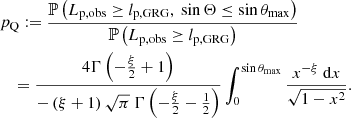


) \cdot f_l^2 \cdot l_\mathrm{p} ^2 \cdot (1 + z)^{3-\alpha }}. \end{aligned} $$](/articles/aa/full_html/2023/04/aa43572-22/aa43572-22-eq66.gif)


![$ \mathbb{E}[L\ \vert\ L_{\mathrm{p}} > l_{\mathrm{p,GRG}}] = \frac{3\pi}{4} l_{\mathrm{p,GRG}} $](/articles/aa/full_html/2023/04/aa43572-22/aa43572-22-eq90.gif)
![$ \mathbb{E}[L\ \vert\ L_{\mathrm{p}} > l_{\mathrm{p,GRG}}] = \frac{16}{3\pi} l_{\mathrm{p,GRG}} $](/articles/aa/full_html/2023/04/aa43572-22/aa43572-22-eq91.gif)


![$$ \begin{aligned} f_L\left(l\right) = {\left\{ \begin{array}{ll} f_L\left(l_\mathrm{ref} \right)\left(\frac{l}{l_\mathrm{ref} }\right)^\xi&l \in [l_\mathrm{min} , l_\mathrm{max} ],\\ 0&\text{ otherwise}. \end{array}\right.} \end{aligned} $$](/articles/aa/full_html/2023/04/aa43572-22/aa43572-22-eq95.gif)


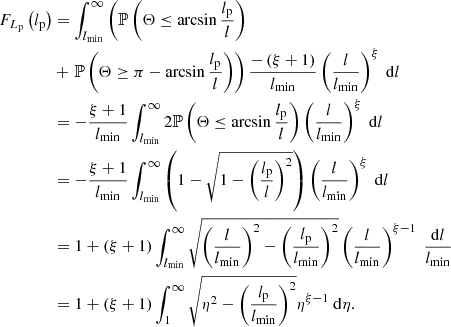
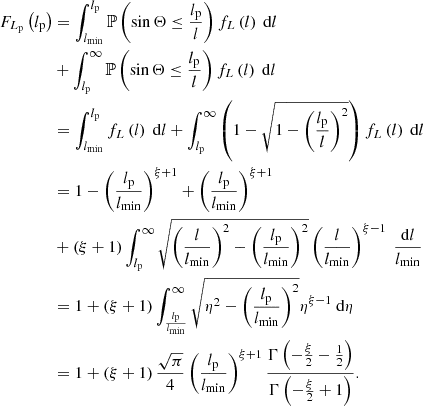


![$$ \begin{aligned} \mathbb{E} [L_\mathrm{p} \ \vert \ L_\mathrm{p} > l_\mathrm{p,GRG} ] :=&\int _{-\infty }^\infty f_{L_\mathrm{p} \ \vert \ L_\mathrm{p} >l_\mathrm{p,GRG} }\left(l_\mathrm{p} \right) \cdot l_\mathrm{p} \ \mathrm{d} l_\mathrm{p} \nonumber \\ =&l_\mathrm{p,GRG} \frac{\xi +1}{\xi +2}. \end{aligned} $$](/articles/aa/full_html/2023/04/aa43572-22/aa43572-22-eq114.gif)

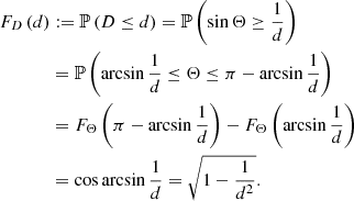


![$$ \begin{aligned} \mathbb{E} \left[D^n\right] = \left(1+\eta \right)^2 I_{n-2}\left(\eta \right) - \eta \left(1+\eta \right) I_{n-1}\left(\eta \right), \end{aligned} $$](/articles/aa/full_html/2023/04/aa43572-22/aa43572-22-eq140.gif)


![$$ \begin{aligned} \mathbb{E} \left[D\right]&= \left(1+\eta \right)^2 I_{-1}\left(\eta \right) - \eta \left(1+\eta \right) I_0\left(\eta \right)\nonumber \\&= \left(1+\eta \right)\left(\frac{\pi }{2} - \frac{\eta }{\sqrt{1-\eta ^2}}\ln {\left(\frac{\sqrt{1-\eta ^2}}{\eta } + \frac{1}{\eta }\right)}\right). \end{aligned} $$](/articles/aa/full_html/2023/04/aa43572-22/aa43572-22-eq143.gif)
![$$ \begin{aligned} \mathbb{E} \left[D^2\right] = \left(1+\eta \right)^2 I_0\left(\eta \right) - \eta \left(1+\eta \right) I_1\left(\eta \right) \end{aligned} $$](/articles/aa/full_html/2023/04/aa43572-22/aa43572-22-eq144.gif)
![$ \mathbb{E}\left[D\right] = \frac{\pi}{2} $](/articles/aa/full_html/2023/04/aa43572-22/aa43572-22-eq145.gif)

![$ \sqrt{\mathbb{V}\left[D\right]} \to \infty $](/articles/aa/full_html/2023/04/aa43572-22/aa43572-22-eq147.gif)


![$$ \begin{aligned} \mathbb{E} \left[L\ \vert \ L_\mathrm{p} = l_\mathrm{p} \right] = l_\mathrm{min} \frac{I\left(\xi , \frac{l_\mathrm{p} }{l_\mathrm{min} }\right)}{I\left(\xi - 1, \frac{l_\mathrm{p} }{l_\mathrm{min} }\right)}. \end{aligned} $$](/articles/aa/full_html/2023/04/aa43572-22/aa43572-22-eq156.gif)
![$$ \begin{aligned} \mathbb{E} \left[L^2\ \vert \ L_\mathrm{p} = l_\mathrm{p} \right] = l_\mathrm{min} ^2 \frac{I\left(\xi + 1, \frac{l_\mathrm{p} }{l_\mathrm{min} }\right)}{I\left(\xi - 1, \frac{l_\mathrm{p} }{l_\mathrm{min} }\right)}, \end{aligned} $$](/articles/aa/full_html/2023/04/aa43572-22/aa43572-22-eq157.gif)
![$$ \begin{aligned} \mathbb{V} \left[L\ \vert \ L_\mathrm{p} = l_\mathrm{p} \right]&= \mathbb{E} \left[L^2\ \vert \ L_\mathrm{p} = l_\mathrm{p} \right] - \mathbb{E} ^2\left[L\ \vert \ L_\mathrm{p} = l_\mathrm{p} \right]\nonumber \\&= l_\mathrm{min} ^2\left(\frac{I\left(\xi + 1, \frac{l_\mathrm{p} }{l_\mathrm{min} }\right)}{I\left(\xi - 1, \frac{l_\mathrm{p} }{l_\mathrm{min} }\right)} - \frac{I^2\left(\xi , \frac{l_\mathrm{p} }{l_\mathrm{min} }\right)}{I^2\left(\xi - 1, \frac{l_\mathrm{p} }{l_\mathrm{min} }\right)}\right). \end{aligned} $$](/articles/aa/full_html/2023/04/aa43572-22/aa43572-22-eq158.gif)
![$$ \begin{aligned} \mathbb{E} \left[L\ \vert \ L_\mathrm{p} = l_\mathrm{p} \right]&= l_\mathrm{p} \cdot \frac{-\xi }{2^{\xi +1}\pi }\frac{\Gamma ^2\left(-\frac{\xi }{2}\right)}{\Gamma \left(-\xi \right)} \int _1^\infty \frac{\eta ^\xi \ \mathrm{d} \eta }{\sqrt{\eta ^2 - 1}}\nonumber \\&= l_\mathrm{p} \cdot \frac{-\xi }{2^{2\xi +3}\pi } \frac{\Gamma ^4\left(-\frac{\xi }{2}\right)}{\Gamma ^2\left(-\xi \right)}. \end{aligned} $$](/articles/aa/full_html/2023/04/aa43572-22/aa43572-22-eq159.gif)
![$$ \begin{aligned} \mathbb{E} \left[L^2\ \vert \ L_\mathrm{p} = l_\mathrm{p} \right] = l_\mathrm{p} ^2 \frac{\xi }{\xi +1}, \end{aligned} $$](/articles/aa/full_html/2023/04/aa43572-22/aa43572-22-eq160.gif)
![$$ \begin{aligned} \mathbb{V} \left[L\ \vert \ L_\mathrm{p} = l_\mathrm{p} \right] = l_\mathrm{p} ^2\left(\frac{\xi }{\xi + 1} - \frac{\xi ^2}{2^{4\xi + 6}\pi ^2}\frac{\Gamma ^8\left(-\frac{\xi }{2}\right)}{\Gamma ^4\left(-\xi \right)}\right). \end{aligned} $$](/articles/aa/full_html/2023/04/aa43572-22/aa43572-22-eq161.gif)


![$$ \begin{aligned} \mathbb{E} \left[\Phi \ \vert \ L_\mathrm{p} > l_\mathrm{p,GRG} \right] = 3 \frac{\xi + 1}{\xi + 4}\left(\frac{1}{\xi + 2} + \frac{1}{2}\right) \cdot \phi _\mathrm{GRG} , \end{aligned} $$](/articles/aa/full_html/2023/04/aa43572-22/aa43572-22-eq177.gif)


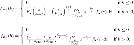


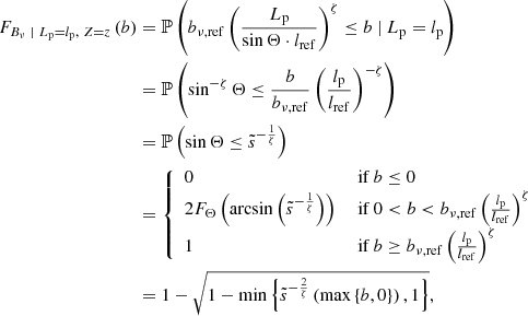


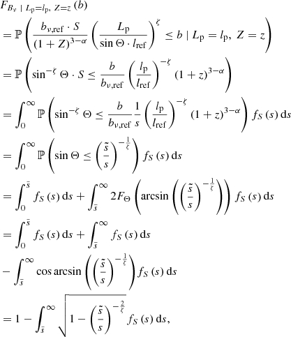


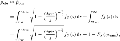
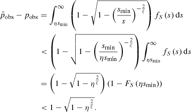


![$$ \begin{aligned} \mathrm{VFF} _\mathrm{GRG} (z=0) :=&\ n_\mathrm{GRG} \cdot \mathbb{E} [V\ \vert \ L_\mathrm{p} > l_\mathrm{p,GRG} ]\nonumber \\ =&\ n_\mathrm{GRG} \cdot \mathbb{E} [\frac{V}{L^3} \cdot L^3\ \vert \ L_\mathrm{p} > l_\mathrm{p,GRG} ]\nonumber \\ =&\ n_\mathrm{GRG} \cdot \mathbb{E} [\Upsilon \cdot L^3\ \vert \ L_\mathrm{p} > l_\mathrm{p,GRG} ]. \end{aligned} $$](/articles/aa/full_html/2023/04/aa43572-22/aa43572-22-eq235.gif)
![$$ \begin{aligned} \mathrm{VFF} _\mathrm{GRG} (z=0)&= n_\mathrm{GRG} \cdot \mathbb{E} [\Upsilon \ \vert \ L_\mathrm{p} > l_\mathrm{p,GRG} ] \cdot \mathbb{E} [L^3\ \vert \ L_\mathrm{p} > l_\mathrm{p,GRG} ]\nonumber \\&= n_\mathrm{GRG} \cdot \mathbb{E} [\Upsilon ] \cdot \mathbb{E} [L^3\ \vert \ L_\mathrm{p} > l_\mathrm{p,GRG} ]. \end{aligned} $$](/articles/aa/full_html/2023/04/aa43572-22/aa43572-22-eq236.gif)
![$$ \begin{aligned} \mathrm{VFF} _\mathrm{GRG} (z=0) > n_\mathrm{GRG} \cdot \mathbb{E} [\Upsilon ] \cdot \mathbb{E} ^3[L\ \vert \ L_\mathrm{p} > l_\mathrm{p,GRG} ], \end{aligned} $$](/articles/aa/full_html/2023/04/aa43572-22/aa43572-22-eq238.gif)
![$$ \begin{aligned} \mathbb{E} [L\ \vert \ L_\mathrm{p} >l_\mathrm{p,GRG} ] = l_\mathrm{p,GRG} \frac{\Gamma \left(-\frac{\xi }{2}-1\right)\Gamma \left(-\frac{\xi }{2}+1\right)}{\Gamma \left(-\frac{\xi }{2}-\frac{1}{2}\right)\Gamma \left(-\frac{\xi }{2}+\frac{1}{2}\right)}. \end{aligned} $$](/articles/aa/full_html/2023/04/aa43572-22/aa43572-22-eq239.gif)
![$$ \begin{aligned} \mathrm{VFF} _\mathrm{GRG} (z=0) > n_\mathrm{GRG} \cdot \mathbb{E} [\Upsilon _\mathrm{p} ] \cdot \mathbb{E} ^3[L_\mathrm{p} \ \vert \ L_\mathrm{p} > l_\mathrm{p,GRG} ] \end{aligned} $$](/articles/aa/full_html/2023/04/aa43572-22/aa43572-22-eq241.gif)
![$$ \begin{aligned} \mathrm{VFF} _\mathrm{GRG} (z=0) > n_\mathrm{GRG} \cdot \mathbb{E} [\Upsilon _\mathrm{p} ] \cdot m_{L_\mathrm{p} ^3\ \vert \ L_\mathrm{p} > l_\mathrm{p,GRG} }, \end{aligned} $$](/articles/aa/full_html/2023/04/aa43572-22/aa43572-22-eq242.gif)

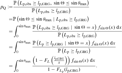


) \cdot f_l^2 \cdot l_\mathrm{p} ^2 \cdot (1 + z)^{3-\alpha }}, \end{aligned} $$](/articles/aa/full_html/2023/04/aa43572-22/aa43572-22-eq256.gif)


